
Submitted:
23 November 2024
Posted:
25 November 2024
You are already at the latest version
Abstract
This work presents an automated weld inspection system based on a one-stage Neural Network trained through a series of 2D weld seam images obtained in the same study. Our method uses You Only Look Once in version 8 (YOLOv8) for object detection. Several models have been trained so that the system can predict: the type of Flux-Cored Arc Welding (FCAW)/Gas Metal Arc Welding (GMAW) weld, two of the common welding processes that have been used in most industries: shipbuilding, automotive, aeronautics among others; detect if a weld is well manufactured or defective; and a third experiment where four classes are attempted to be detected: a correctly manufactured weld, if it presents a lack of penetration defect, an undercut defect or other manufacturing problems. The presented system does not stop at determining the correct welding parameters. The study is based on finding a robust and reliable system to support this difficult and critical task of weld inspection. High performance was achieved in all three experiments carried out in this study, both in those that established a binary classification (the first two) and in the one that established a multiclass classification (the third experiment). In all of them, an average prediction success rate of over 97\% was achieved.
Keywords:
CNN
; surface inspection welding
; shipbuildig
; FCAW
; GMAW
; welding defects
; deep learning
; yolo
1. Introduction
One of the most important tasks in the welding production process is the subsequent inspection of the work performed. Being the time invested in this activity much higher in relation to the welding task itself.
Nowadays, the welding process is established in many sectors of the industry. For each of these industries there are a number of ISO standards rules that must be met for welding work to be accepted. There are industries such as the naval sector where the critical level of importance of welding is maximum. That is why welding testing tasks must be as important as the welding task itself. The cost of welding inspection, both temporary and economic, represents a fairly high percentage with respect to the welding work itself [1].
1.1. Background
Nevertheless, the task of visual inspection of the weld begins once the weld seam has already been created, so for a study of this type, what is truly important is to apply some type of technique to check the goodness of the created seam. In this sense, there are several techniques to carry out this inspection work, within what are called non-destructive tests: ultrasonic testing, radiographic testing, magnetic testing, and the simplest technique that involves visually observing the welding carried out by an expert, among others.
Although the most widely used technique is radiographic testing, direct visual inspection by an expert is still widely used. In any case, due to the number of meters of welding that must be checked and the large amount of time that must be devoted to this task, it is necessary to automate it to the maximum, achieving acceptable automation reliability.
Due to the importance, due to the relevance of the processes, and due to its use in the industry, this work focuses on the study of the FCAW and GMAW welding processes.
In this way, FCAW is an electric arc welding process in which the arc is established between the continuous tubular electrode and the piece to be welded. The protection is carried out through the decomposition of raw materials contained in the tube, with or without external gas protection and without applying pressure [2], as can be seen in Figure 1. On the other hand, GMAW is an arc welding process that requires automatic feeding of an electrode protected by a gas that is supplied externally [3], as can be seen in Figure 2.
Without a doubt, the study of the input parameters in robotic welding, as is the case of the works presented in [5,6] is a determining factor when it comes to obtaining a weld bead of acceptable quality by current regulations, as the authors mention in [7]. However, in the presented work we will focus on solving the use of applying a neural network on images of weld seams, with the intention of detecting possible defects and well-made seams.
1.2. Related works
For some years now, various methods and models used by other authors have been appearing to address the task of inspection, monitoring or diagnosis of a weld based on the concept of neural networks, in its various variants. These methods have been used in various welding processes in various sectors. As the authors indicate in [8], they propose a real-time monitoring system for laser welding of tailor rolled blanks using Convolutional Neural Network (CNN). In another study [9], an Artificial Neural Network (ANN) is used, in this case, to obtain a prediction of welding residual stress and deformation in electro-gas welding. There are studies that are somewhat closer to what is discussed in this paper. As is the case of [1], where the authors propose the detection of weld defects using a type of CNN called Faster R-CNN, trained with X-rays images of the weld seams. In [10] also offers you a Welding Surface Inspection of Armatures system through CNN and image comparison. In the same way in [11], the authors detect defects in the GMAW welding process through Deep Learning (DL), using ultrasonic, magentoscopic, and penetrant liquids tests were performed on the welds techniques, although they do not share the dataset used.
The reviewed studies sometimes use their own images to train their artificial neural networks. On other occasions, the works themselves, such as the one presented, have created a dataset of images for the occasion, as is the case of [12]. Where a database of X-ray images corresponding to five categories is incorporated: castings, welds, baggage, natural objects and settings. Created for the training itself, in [13] proposes a camera-based system where a series of images of welding seams are created using a certain sensor, training a CNN from them. In the case of [14] and [15], the authors propose an unsupervised learning model using their own radiographic images and other calculations. In the same way, the authors in [16] create their own dataset of radiographic images to train a DL system based on VGGnet [17].
Traditionally, neural network architectures for object detection are often divided into two categories called one-stage or two-stage. In two-stage detector methods, a Region Proposal Network (RPN) is created. RPN is used for generating high-quality object proposals which are very vital to improve the performance of detectors [18,19]. This RPN is used to generate the Regions Of Interest (ROI), proposed in the first stage. These ROI proposals are subsequently used for classification and bounding box regression in the second stage. Two-stage methods have the disadvantage that they are usually slower, however they have higher precision than one-stage methods. On the other hand, one-stage detectors do not preselect to generate candidates like two-stage methods. They directly attempt to detect the objects by solving a simple regression problem. That is why one-step methods are faster in their resolution, but produce results with less precision [20]. In the same way, Single Shot Detection (SSD) is presented by its authors [21] as a method to detect objects in images using a single deep neural network, in a single stage. In this case, the output bounding boxes are discretized into a set of already predefined boxes using various aspect ratios and scales, locating the position on the feature map. Predicting the network generates scores for each category of object in each default box and produces adjustments to the box to better match the shape of the object.
Thus, within the one-stage methods studied, the most interesting and traditionally used, which can be highlighted are YOLO [22]. This method is responsible for solving the object detection problem by applying a regression to bounding boxes that are separated in space, together with the application of class probabilities associated with the boxes. From here, a single neural network predicts class probabilities and bounding boxes from full images. RetinaNet is a one-stage method, however it is able to achieve the precision of two-stage methods without losing the speed of its class methods, because it addresses the class imbalance between foreground and background [20].
Methods based on a two-stage approach are more common and widespread within the world of DL object detection. Thus, R-CNN [23] is made up of three parts. In the first, proposals for independent candidate regions of each category are generated. The second part is made up of one that extracts features of fixed length. The third part is a set of SVMs The second module is a large convolutional neural network that extracts a feature of fixed length vector of each region. The third module is a set of class-specific linear Support Vector Machines (SVMs). R-FCN, where fully convolutional region-based networks are presented for accurate and efficient object detection. Unlike other models like Fast/Faster R-CNN, which apply a costly subnet per region hundreds of times, in this case the calculations are shared across the entire image, proposing scoremaps relative to position [24]. In the case of Fast R-CNN, this method is based on efficiently classifying object proposals using deep convolutional networks. Compared to previous works, Fast R-CNN brings innovations to improve training and test speed, while increasing object detection accuracy [25]. Faster R-CNN [26], where an RPN is presented that shares convolutional characteristics with the detection network. We already know that an RPN is a fully convolutional network capable of predicting both object limits and object scores at each position. In this case, the RPN generates high-quality region proposals, which Fast R-CNN uses for detection, merging RPN and Fast R-CNN into a single network that shares features, making a substantial improvement on the latter. Or Mask-RCNN [27], which extends from Faster R-CNN by adding a branch to predict an object mask in parallel with the existing branch that recognizes bounding boxes.
After searching the existing bibliography, some articles have been located that deal with the creation and provision of image datasets focused on the detection of weld defects. Thus, in the first place we mention the GDXray database, free to use, that the authors present in [12]. It is a database of images taken with X-rays, intended to perform non-destructive tests, not being explicitly of welding defects.
The authors in [24], although they do not make the image repository public, propose the creation of an image database, where the frequency even appears, to detect defective spot welds. They focus on studying performance in small datasets and with unbalanced classes, the images being taken with a high resolution camera. In the same way, taking the images with a high resolution color camera, in the work presented in [10], the authors propose a welding surface inspection of armatures. They use a CNN-based approach. comparing various CNN models against each other. In both cases, the authors do not make the image dataset public so that it can be studied in other research.
The investigation carried out in [28] shows a radiographic imaging to detect welding defects in shipbuilding. Although the authors show us the number of images taken, the percentage composition of the train, validation and test groups, there is no reference reference to said dataset.
Definitely, some previous research has been found for automated recognition of surface weld defects based on DL. In few works, new datasets are used, or the data used for training is not offered publicly. The dataset, or collection of data, most used and which can be accessed is the GDXray database, already referenced in the previous paragraph.
1.3. Contribution
Thus, to our knowledge, there is no study for the detection of fillet weld defects using convolutional neural networks trained with images taken with a 2D camera. Therefore, the main contributions of the work are the following:
- A set of images of weld seams has been created and made available to the scientific community, where there are images of accepted seams and seams that have some defect: lack of penetration, bites and lack of fusion. These images have been taken with FCAW and GMAW welding differently. The images are captured with a 2D cam, instead of X-ray images, as has traditionally been done in other works.
- The development of a methodology that can be used in other works based on image detection.
- The study and results of three experiments based on the application of neural networks through the analysis of 2D images: the detection of the type of FCAW/GMAW weld, the verification of the goodness of a weld and the detection of certain defects in a weld seam.
1.4. Organization
Section 2 the materials and methods used are described, where we will detail the materials and the process that has been established to define, the methodology and the steps that have been followed to carry out this research. Next, in Section 3, the results and conclusions of this work will be presented. Ending with Section 4, with the conclusions of future work.
2. Materials and Methods
Throughout this section will detail the framework used in the research. In our experimentation we need a framework that allows us to create the welding seams and another one that is capable of allowing us to acquire images to train the neural network. Next, the methodology used in the research will be explained. These steps will be explained appropriately so that they can be used in other projects or research related to object detection.
2.1. Framework
The case study focuses on the manufacture of fillet welds on steel plates, using two welding techniques, FCAW and GMAW. Thus, the FCAW and GMAW welding processes were configured on a FANUC LR Mate 200 iD 7L robotic arm (Fanuc, Japan), Figure 3a, equipped with a Lincoln R450 CE welding system (Lincoln Electric, USA), as can be seen in Figure 3b, the wire and gas necessary to achieve a correct weld according to the mentioned processes. The shield gas combination used in the manufacture of the weld seams was composed of 80% argon and 20% carbon dioxide for the GMAW welding process, and 75% argon and 25% carbon dioxide for the FCAW process, because they are the combinations that present a greater balance with regard to the reliability of the weld and its final quality, according to the type of steel used in the experiment, as can be seen in [29].
Weld seams of approximately 5-7 cm were created in one-pass weld, on 6 mm thick steel plates, by welding in a L-shape, fillet weld, as can be seen in Figure 4, where you can see five weld seams. Subsequently, each seam was numbered and labeled as acceptable or not acceptable. And within the non-acceptable option, its manufacturing defect was labeled. The labels were assigned by two human welding experts, who inspected each seam visually, as would be done in typical surface inspection welding field work.
Next, the study continues with a series of images of these welds will be obtained in order to train a neural network. Once this network has been trained, a single-step Deep Learning architecture, YOLOv8, will be used to predict the type of weld performed and the welding defects found. Thus, the pictures have been taken in different tones of light, aided by the luminaire that appears in Figure 5a. When automating the process of taking images and their capture positions, these were taken by placing the high-resolution camera used in the end effector of a robotic arm, as can be seen in Figure 5b. In this way, it is intended that the dataset is as complete as possible, and that the learning is not so strict.
2.2. Methodology
To carry out the experiments of this study, a series of steps were carried out as can you seen in Figure 6. As it can be seen there, the raw images are taken. This data acquisition (DA) is carried out by taking images of the weld beads created, according to the framework described above. Next, the characteristics of each bead (FE) will be extracted according to the dataset to be built. Thus, the corresponding bounding boxes will be created in each image, indicating the parts of the image that are to be trained, according to the established classes. For each dataset created, the same data preprocessing (DP) techniques will be applied from among all those that exist, as well as the application of the same Data Augmentation (DAU) techniques. In the present study, three datasets were constructed for the purpose of investigating three distinct object recognition models.
The next step will be to select the training/validation data set, to which a series of hyperparameters (HS) will be applied based on other works studied in the bibliography of the DL model with which we work.
Next, we will apply the DL model that we have used in this research, YOLO, and we will take the performance metrics that we consider most appropriate to study in this paper (PM).
2.2.1. Data Acquisition (DA)
As in any training, it is essential to have the most perfect data possible. Therefore, we focused mainly on obtaining 2D images of the welding seams of the highest quality and precision, in accordance with the experiment that was going to be carried out.
The images, which constitute our initial data, represent the most crucial element of an object recognition system based on deep learning techniques. The images were captured using a high-resolution camera, as illustrated in Figure 7. The camera was placed on the end effector of a robotic arm, with the aim of taking a total of seven poses of each weld bead, with different luminosities, in order to have more images for the training/validation/test dataset. To do this, a simple program was created in the robot, where it had seven stopping points, taking an image of the weld beads at each of these points.
The camera was placed on the end effector of a robotic arm, with the aim of taking a total of seven poses of each weld bead, with different luminosities, in order to have more images for the training/validation/test dataset. To do this, a simple program was created in the robot, where it had seven stopping points, taking an image of the weld beads at each of these points, as you can see in Figure 5b.
2.2.2. Feature Extraction (FE)
The structures used are made of mild steel, which is a material widely used in certain industries such as shipbuilding. This material stands out among other properties for its high tensile strength, which guarantees the integrity of the structure and serves as an excellent support for creating weld beads, making reliable joints [30]. A complicated scene is therefore presented, because there is a steel plate or structure, joined by a weld bead, both with similar material and visual characteristics.
Therefore, it is essential to select the scene that the system wants to learn well. For this reason, the boundary box process, or labeling, has been carried out on each image of each dataset created, using an appropriate online tool for this, Roboflow [31]. In this way, it has been possible to label each of the characteristics that have been studied in the research in each dataset. Thus, for each dataset a series of labels or classes will be specified that will be selected in each raw image. These labels will correspond to the learning and search characteristics that you want to train in the model.
In Figure 8 you can see one of the welded and suitably labeled steel plates, indicating to the system, in this case, the welds that are well manufactured (good label) and those that have some defect (bad label).
2.2.3. Data Preprocessing (DP)
Although it may seem like a secondary step, some image preprocessing techniques can help detect the objects we intend to find in each scene [32]. Among other techniques we can find: grayscale, image self-orientation, contrast adjustment, size readjustment,...
In our case, the images have already been taken in high quality grayscale, so it is not necessary to apply this preprocessing. However, we consider it to be one of the most important transformations, since the system is able to converge in the same way to detect objects as if the image were taken in color, but investing less computing power due to the absence of color channels.
We consider it important, so that the system can converge better, to apply a single and equal size to each image, so a size readjustment has been applied to each image. Likewise, a self-orientation of each image has been applied so that the system can train with a more solid pattern.
2.2.4. Data Augmentation (DAU)
Data augmentation is a very effective method for creating useful DL models. This method ensures that the validation error should decrease along with the training error. It achieves this by representing a more complete set so that it is able to minimize the distance between the training and validation data, including the test set [33]. The augmentation techniques applied included the following:
- Horizontal flips: This effect will reflect the images horizontally increasing the variety of vertex orientations.
- Shear: add variability to perspective to help the model be more resilient to camera and subject pitch and yaw.
- Noise: the noise to help our model be more resilient to camera artifacts.
These data augmentation techniques will improve the robustness of the model, particularly the detection of small objects such as welding seams. The training data set will be expanded with several variations on the original images. In this way, the model will learn to generalize better and to be more resistant to changes in lighting, image quality or orientation, among others.
In this study, the size of the data set has been intentionally limited, since it is a proof of concept. However, at the production level this data set must be increased in order to obtain a more robust model, better prepared for changes and to increase its precision and generalization.
2.2.5. Hyper-parameters Selection (HS)
Within a YOLO system there are a series of hyperparameters that can be configured according to the training to be performed. Table 1 lists the hyperparameters that have been used in each of the three experiments performed in this research.
In order to select the hyperparameters for each experiment, it has been taken into account that they are as homogeneous as possible, so that a comparison and discussion of the results can be made as fair as possible later. Thus, only the number of epochs has been altered between one experiment and another, due to the complexity of the detection and the characteristics of the classes to be detected, which have led to a slower convergence of the model. In any case, the lowest possible number of epochs has been applied, to avoid possible overfitting, taking into account that we have a limited dataset.
During training, a batch size of 16 was used, meaning it was updated after simultaneously processing 16 images. The choice of this parameter was based on the available resources. A larger batch size could improve training speed, but may require more memory.
The learning rate was set to 0.01. This parameter controls the tuning of the model weights during each training iteration. Care must be taken in choosing it, as a higher learning rate might result in faster convergence, but at the same time it could lead to oscillations or exceeding the optimal weights.
The stochastic gradient descent (SGD) optimizer was employed. The SGD is a classic optimization algorithm that iteratively updates the model’s weights based on the gradient of the loss function.
The input images were resized to 320 x 320 pixels, which is a lower resolution than the one commonly used for YOLO models. Due to the characteristic of the image to be detected, it was considered convenient not to invest in a larger image size, in order to guarantee a consistent input size for the model and efficient in terms of training time and memory occupied.
The confidence threshold is represented as the inverse of the significance threshold and is also often expressed as a percentage. Confidence determines how confident the model is that a prediction matches the true value of a class. The threshold determines the value to label a class as that class. So, let’s say we have a confidence threshold of 0.6, this means that the model will have to be at least 60% confident that the object it is trying to classify is that object before it gets around to labeling it. In our case, we have required a confidence of 0.75, so we will have to ensure that the predictions are at least 75% certain. This value is interesting to use when we are sure that the model converges well with a high percentage of success.
Additionally, note that the MS COCO [34] weights have been used, which were passed as input parameters to the YOLO algorithm.
2.2.6. Deep Learning Model (DLM)
For this work we have investigated to find a deep learning model that was robust, efficient, accurate and fast. We had previously detected non-conventional objects, such as a weld bead, so the detection would be somewhat specific. Once we had reviewed the literature for the two traditional ways of tackling a problem based on DL, such as one-stage and two-stage detect methods, we decided to opt for YOLO, a real-time object detection system that meets all the characteristics we were looking for.
Once the datasets were created according to the areas and characteristics we wanted to detect, a YOLO model was trained for each of them, in total three, with the following detections:
- Differentiate the type of weld used in the manufacture of the weld (FCAW/GMAW).
- Detect whether the weld has been manufactured correctly, according to the standards that a human viewer would have taken into account, regardless of the type of weld used.
- Determine whether the weld has been manufactured correctly. If not, recognize the type of defect that the weld bead has: undercut, lack of penetration, other problems.
Of all the versions of YOLO, the YOLOv8 version has been used, that gives the best results taking into account the characteristics sought, noted above. This version was released by a company, Ultralitycs, that develops models and tools to build, optimize and implement deep learning models. Specifically, YOLOv8 was designed to detect small objects, improve localization accuracy and improve the performance-to-computing ratio, which makes it even more ideal for the purpose of our work. In addition, as can be seen in [35], all the characteristics of YOLO: performance, precision, robustness, efficiency,... are far superior to its predecessors.
2.2.7. Performance Metrics (PM)
In order to demonstrate the rigor of this research and to be able to measure the performance of the YOLO algorithm used by making a fair and reliable comparison, the following metrics have been defined:
-
Recall (R). It is also called sensitivity or TPR (true positive rate), representing the ability of the classifier to detect all cases that are positive, Equation 1.TP (True Positive) represents the number of times a positive sample is classified as positive, i.e. correctly. On the other hand, FN (False Negative) tells us the number of times a negative sample is classified incorrectly.
-
Precision (P). Controls how capable the classifier is to avoid incorrectly classifying positive samples. Its definition can be seen in Equation 2.In this case, FP (false positive) tells us how many times negative samples are classified as positive.
- Intersection over union (IoU) is a critical metric in object detection as it provides a quantitative measure of the degree of overlap between a ground truth (gt) bounding box and a predicted (pd) bounding box generated by the object detector. This metric is highly relevant for assessing the accuracy of object detection models and is used to define key terms such as true positive (TP), false positive (FP), and false negative (FN). It needs to be defined because it will be used to determine the mAP metric. Its definition can be seen in Equation 3.
-
Mean Average Precision (mAP). In object detection is able to evaluate model performance by considering Precision and Recall across multiple object classes. Specifically, mAP50 focuses on an IoU threshold of 0.5, which measures how well a model identifies objects with reasonable overlap. Higher mAP50 scores indicate better overall performance.For a more comprehensive evaluation, mAP50:95 extends the evaluation to a range of IoU thresholds from 0.5 to 0.95. This metric is appropriate for tasks that require precise localization and fine-grained object detection.mAP50 and mAP50:95 are able to help evaluate model performance across multiple conditions and classes, thereby expressing information about object detection accuracy by considering the trade-off between Precision and Recall.Models with higher mAP50 and mAP50-95 scores are more reliable and suitable for demanding applications. These are appropriate metrics to ensure success in projects such as autonomous driving and safety monitoring.Equation 5 shows the calculation of Average Precision, which is necessary to calculate the mean Average Precision (mAP), which can be seen in the equation.
- Box loss: This loss helps the model to learn the correct position and size of the bounding boxes around the detected objects. It focuses on minimizing the error between the predicted boxes and the ground truth.
- Class loss: It is related to the accuracy of object classification. It ensures that each detected object is correctly classified into one of the predefined categories.
- Object loss: It is related to the accuracy with which objects are classified. It ensures that each detected object is correctly classified into one of the predefined categories. That is, object loss is responsible for choosing between objects that are very similar or difficult to differentiate, by better understanding their characteristics and spatial information.
3. Results and Discussion
In this section, the suitability of the proposed methodology for recognizing welding seams will be validated according to three experiments presented in this research. Next, the experimental environment is described below, the results are shown and discussed.
3.1. Experimental environment
An experimental environment has been designed to execute the proposed methodology. The methods and functions have been developed in Python language. Additionally, a set of tools such as the algorithm called YOLO in its version 8, and roboflow [31] for labeling the images of the dataset that has been created in this study were used. To award the labels in each experiment carried out, the visual assessment of two welding experts was taken into account, who analyzed each of the welded plates and determined, based on their experience and criteria in visual inspection of welding beads, whether a weld was well manufactured (GOOD), poorly manufactured (BAD), weld manufactured with the FCAW or GMAW method, or weld manufactured with any of the defects studied, undercut (UNDER), lack of penetration (LOP), or rest of defects (OP). In addition, YOLO Ultralitycs [36,37] has been used for performance metrics.
The dataset used in this study has been presented in Section 2.1. The suitably labeled images have been selected to be validated using the YOLO algorithm. This algorithm initially needs to learn the location of the object to be searched for within the set of images. Therefore, 80% of the images have been provided for training and 20% for testing. From this set of 80%, 10% has been selected as the validation set.
Although more types of defects could have been detected in the images of the weld beads that make up the dataset, it has been decided to recognise the two most important ones, lack of penetration and underbite, leaving the rest for a class called “other problems (op)”. The reason why other defects have not been taken into account is because the weld beads were manufactured by a welding robot. This means that the weld beads are manufactured correctly, and in the case that they are defective (generally due to a bad parameter assignment) the defects produced are mostly those that have been studied. The rest of the defects occur on a small number of occasions. Having taken them into account separately would have meant having a very small set of samples, and could have negatively influenced the performance of the detection and classification of the weld seams.
The experiments presented in this study have been carried out at the facilities of the supercomputing center of the University of Cadiz, which has 48 nodes, each with two Intel Xeon E5 2670 2.6 GHz octa-core processors, equipped with 128 GB of RAM.
3.2. Experiments Results and Discussion
Throughout this subsection, each of the experiments that have been carried out to validate the effectiveness of using the YOLOv8 algorithm in detecting weld seams according to the proposed methodology will be explained. In each of the experiments, the obtained results are introduced both numerically and graphically.
Table 2 contains the numerical data for the metrics used to evaluate the performance of our study. For each of the experiments performed, Recall, Precision and mAP are shown. The performance obtained for this last metric is shown both in the validation set and in the training set. Each of the experiments carried out is detailed below.
3.2.1. Experiment 1: FCAW-GMAW Weld Seam
Although at first glance it is possible to differentiate between FCAW and GMAW welding types, it is a difficult task to perform for someone who is not trained in the world of welding. For this reason, we proposed the possibility of an automated system that could detect the type of welding with which a particular welding bead was created.
For this dataset [38] the weld seams were cropped from the plates shown in Figure 4, so that the model was trained on a labeled image that contained almost only the bead to be detected. The images in this dataset barely have more space than the bead itself and, although the size is standard (320x320), the appearance is irregular as can be seen in Figure 9, where a set of these images is displayed. Two classes of object to be detected were therefore established, FCAW and GMAW.
In the first row of the Table 2, it can be observed that the performance of all the metrics is above 98% in all of them. Only the test set of the mAP metric was at 93%, which perhaps made the model take a little longer to converge. Nevertheless, 100 epochs were enough for the model to converge.
Figure 10 shows the results after training of the first experiment, FCAW-GMAW detection. The training loss curves for bounding box, classification, and confidence score prediction decreased significantly over the 75 epochs, indicating that the model learned effectively. The model achieved good performance with high precision (around 0.98), recall (around 0.98), and mAP scores (reaching around 0.97 for mAP50). This suggests that the trained model was able to accurately detect the weld bead, whether it was created using the FCAW or GMAW technique. That is, the model was able to find characteristics specific to each welding method, in order to differentiate them.
3.2.2. Experiment 2: Good-Bad Weld Seam
In this second experiment, it was considered convenient and interesting to carry out a binary classification where the model can detect a well-manufactured welding bead and a poorly manufactured welding bead, without taking into account, on this occasion, the welding process used as we did take into account in experiment 1.
In the dataset created for this experiment [39], labels (GOOD-BAD) have been established on each of the plates, which contain more than one welding bead, correctly created beads and incorrectly created beads were included, so that the model could obtain better learning, as can be seen in Figure 11.
In the second row of Table 2, we can see the data for the performance metrics obtained for this second experiment. We can see how all of them have maintained a high score, similar to the scores obtained in the first experiment. Even higher data in Precision and Recall, being noticeably lower in the validation set of the “good” class, which can lead us to think that the model has had more difficulties in classifying this class.
Figure 12 shows the training curves and performance metrics of the model trained in this second experiment. If we look at the curves, we can see how the model reaches convergence in a more regular and uniform way than in experiment 1. In this case, for each epoch the loss improves in each one of them, a situation that did not occur in the first experiment, in which there were epochs that showed worse results than later epochs. However, 300 epochs were needed in this experiment to achieve correct model learning, although at approximately epoch 200 the learning is already stabilizing.
3.2.3. Experiment 3: Good-Lop-Under Weld Seam
In order to carry out a more complex experiment, which could detect more than two classes, and at the same time have an importance within the field we are investigating, we created this third experiment. In it, we wanted to make a brief study of the defects that a weld bead can have when it is manufactured, detecting two of the most common ones: undercuts and lack of penetration, creating another additional class to detect other welding problems, and thus differentiate these welds from well-manufactured welds. Thus, the detection of a correctly manufactured weld, or the detection of defects: undercuts (UNDER), lack of penetration (LOP) and other problems (OP), together with the class of correct welds (GOOD) was proposed.
In the second row of Table 2 we can see the data for the performance metrics obtained for this second experiment. We can see how all of them have maintained a high score, similar to the scores obtained in the first experiment. Even higher data in Precision and Recall, being noticeably lower in the validation set of the “good” class, which can lead us to think that the model has had more difficulties in classifying this class. The performance in the rest of the mAP metrics is very similar to that obtained in previous experiments.
For this third experiment, a dataset [40] has been created where four objects (GOOD-UNDER-LOP-OP) corresponding to well-manufactured welds, the first of the classes, and several defects, the other three classes, are intended to be detected. Figure 13 shows a plate with several fillet weld seams, each of them labeled by the model.
Figure 14 shows the training curves and performance metrics of the model trained in this third experiment. The curves show that the model does not follow a uniform trend, and that it has difficulty adjusting the loss in the first epochs. This may be because in this experiment the model has to detect four classes and the number of samples is not very high. A total of 300 epochs were used to achieve effective learning. However, as in the previous experiment, from epoch 200 onwards the learning stabilises until reaching maximum efficiency. In this experiment, as in the previous ones, a sufficient number of epochs have been used, in order to avoid overfitting.
4. Conclusions and Future Work
In this paper, a study has been carried out on the detection of fillet weld beads according to certain criteria, from a series of 2D images, also taken in this study. From the treatment of the images and the creation of several datasets, a series of experiments have been carried out in order to detect types of welds, goodness of manufacture of the weld bead or certain defects. Object detection has been focused using the YOLOv8 algorithm, properly configuring some of its hyperparameters and applying a specific methodology developed for this study.
Thus, after the three experiments carried out, it is demonstrated that the YOLOv8 algorithm is effective for the detection of fillet weld beads, since a prediction performance of over 97% is achieved in all the characteristics studied. Although it is true that as detection has become more complicated, with more difficult classes to detect, or with a number of class detections greater than two in the same experiment, performance has been noticeably lower. However, it seems that there is still room in the percentage of performance to create a model that is capable of detecting a series of weld beads with multiple characteristics.
The present study, like other similar ones related to object detection, may have as a limitation the fact that the images obtained in another system and that are intended to be inferred by the model trained here, despite taking the same steps as explained in the methodology and the same precautions when taking the photos, it is likely that the detection of objects is defective, or at least, a lower performance than that obtained in this study is obtained. That is why, as future work, we propose to use Transfer Learning techniques, based on this research, to try to detect other types of welding beads, made with other processes. Thus, the checkpoints obtained in this research could be used to detect other welding beads created in another experiment. On the other hand, for the Data Augmentation phase, it would be interesting to apply a more complex technique such as GAN networks, and measure how it affects the performance of the detection of defects in welding beads. It would also be possible, as future work, to increase the size of the dataset, with the aim of detecting more characteristics related to fillet welding or another type of welding.
Author Contributions
Conceptualization, J.M.R.C., A.M.-E., I.D.-C. and P.M.-C.; data curation, B.S.-D. and I.D.-C.; formal analysis, M.A-A. and J.M.R.C.; funding acquisition, A.M.-E. and M.A.-A.; investigation, P.M.-C., A.M.-E., I.D.-C. and B.S.-D.; methodology, B.S.-D. and M.A.-A.; project administration, A.M.-E. and I.D.-C.; resources, A.M.-E. and M.A.-A.; software, P.M.-C. and I.D.-C.; supervision, A.M.-E. and M.A.-A.; validation, J.M.R.C. and I.D.-C.; visualization, A.M.-E. and P.M.-C.; writing—original draft, B.S.-D. and I.D.-C.; writing—review and editing, I.D.-C., B.S.-D. and J.M.R.C. All authors read and agreed to the published version of this manuscript.
Funding
This research received no external funding.
Informed Consent Statement
Not applicable.
Data Availability Statement
Conflicts of Interest
The authors declare no conflict of interest.
Abbreviations
The following abbreviations are used in this manuscript:
| YOLO | You Only Look Once |
| CNN | Convolutional Neural Network |
| RPN | Region Proposal Network |
| GMAW | Gas Metal Arc Welding |
| FCAW | Flux Cored Arc Welding |
| ANN | Artificial Neural Network |
| DA | Data Acquisition |
| FE | Feature extraction |
| DP | Data Preprocessing |
| DAU | Data Augmentation |
| DL | Deep Learning |
| NAS | Neural Architecture Search |
| PM | Performance Metrics |
| R | Recall |
| P | Precision |
| TP | True Positive |
| FP | False Positive |
| gt | Ground Truth |
| pd | Predicted Box |
| IoU | Intersection over Union |
| AP | Average Precision |
| mAP | Mean Average Precision |
| TEP940 | Applied Robotics Research Group of the University of Cadiz |
| ROI | Region Of Interest |
| SSD | Single Shot Detector |
References
- Oh, S.J.; Jung, M.J.; Lim, C.; Shin, S.C. Automatic detection of welding defects using faster R-CNN. Applied sciences 2020, 10, 1–10. [Google Scholar] [CrossRef]
- Mohamat, S.A.; Ibrahim, I.A.; Amir, A.; Ghalib, A. The Effect of Flux Core Arc Welding (FCAW) Processes On Different Parameters. Procedia Engineering 2012, 41, 1497–1501. [Google Scholar] [CrossRef]
- Ibrahim, I.A.; Mohamat, S.A.; Amir, A.; Ghalib, A. The Effect of Gas Metal Arc Welding (GMAW) Processes on Different Welding Parameters. Procedia Engineering 2012, 41, 1502–1506. [Google Scholar] [CrossRef]
- Hernández Riesco, G. Manual del soldador 28a Edición; Cesol, Asociación Espańola de Soldadura y Technologías de Unión, 2023.
- Katherasan, D.; Elias, J.V.; Sathiya, ·.P.; Haq, ·.A.N. Simulation and parameter optimization of flux cored arc welding using artificial neural network and particle swarm optimization algorithm. J Intell Manuf 2014, 25, 67–76. [Google Scholar] [CrossRef]
- Ho, M.P.; Ngai, W.K.; Chan, T.W.; Wai, H.w. An artificial neural network approach for parametric study on welding defect classification. The International Journal of Advanced Manufacturing Technology 2021, 1, 3. [Google Scholar] [CrossRef]
- Kim, I.S.; Son, J.S.; Park, C.E.; Lee, C.W.; Prasad, Y.K. A study on prediction of bead height in robotic arc welding using a neural network. Journal of Materials Processing Technology 2002, 130-131, 229–234. [Google Scholar] [CrossRef]
- Zhang, Z.; Li, B.; Zhang, W.; Lu, R.; Wada, S.; Zhang, Y. Real-time penetration state monitoring using convolutional neural network for laser welding of tailor rolled blanks. Journal of manufacturing systems 2020, 54, 348–360. [Google Scholar] [CrossRef]
- Liu, F.; Tao, C.; Dong, Z.; Jiang, K.; Zhou, S.; Zhang, Z.; Shen, C. Prediction of welding residual stress and deformation in electro-gas welding using artificial neural network. Materials today communications 2021, 29, 102786. [Google Scholar] [CrossRef]
- Feng, T.; Huang, S.; Liu, J.; Wang, J.; Fang, X. Welding Surface Inspection of Armatures via CNN and Image Comparison. IEEE sensors journal 2021, 21, 21696–21704. [Google Scholar] [CrossRef]
- Nele, L.; Mattera, G.; Vozza, M. Deep Neural Networks for Defects Detection in Gas Metal Arc Welding. Applied Sciences 2022, Vol. 12, Page 3615 2022, 12, 3615. [Google Scholar] [CrossRef]
- Mery, D.; Riffo, V.; Zscherpel, U.; Mondragón, G.; Lillo, I.; Zuccar, I.; Lobel, H.; Carrasco, M. GDXray: The Database of X-ray Images for Nondestructive Testing. Journal of nondestructive evaluation 2015, 34, 1–12. [Google Scholar] [CrossRef]
- Hartung, J.; Jahn, A.; Stambke, M.; Wehner, O.; Thieringer, R.; Heizmann, M. Camera-based spatter detection in laser welding with a deep learning approach. Forum Bildverarbeitung 2020. Ed.: T. Längle ; M. Heizmann 2020, pp. 317–328. [CrossRef]
- Nacereddine, N.; Goumeidane, A.B.; Ziou, D. Unsupervised weld defect classification in radiographic images using multivariate generalized Gaussian mixture model with exact computation of mean and shape parameters. Computers in industry 2019, 108, 132–149. [Google Scholar] [CrossRef]
- Deng, H.; Cheng, Y.; Feng, Y.; Xiang, J. Industrial laser welding defect detection and image defect recognition based on deep learning model developed. Symmetry (Basel) 2021, 13, 1731. [Google Scholar] [CrossRef]
- Ajmi, C.; Zapata, J.; Martínez-Álvarez, J.J.; Doménech, G.; Ruiz, R. Using Deep Learning for Defect Classification on a Small Weld X-ray Image Dataset , 2020. [CrossRef]
- Simonyan, K.; Zisserman, A. Very Deep Convolutional Networks for Large-Scale Image Recognition. Symmetry 2014. [Google Scholar]
- Wang, R.; Jiao, L.; Xie, C.; Chen, P.; Du, J.; Li, R. S-RPN: Sampling-balanced region proposal network for small crop pest detection. Computers and Electronics in Agriculture 2021, 187, 106290. [Google Scholar] [CrossRef]
- Ren, S.; He, K.; Girshick, R.; Sun, J. Faster R-CNN: Towards Real-Time Object Detection with Region Proposal Networks. In Proceedings of the Advances in Neural Information Processing Systems; Cortes, C.; Lawrence, N.; Lee, D.; Sugiyama, M.; Garnett, R., Eds. Curran Associates, Inc., 2015, Vol. 28.
- Wang, Y.; Shi, F.; Tong, X. A Welding Defect Identification Approach in X-ray Images Based on Deep Convolutional Neural Networks. In Proceedings of the Intelligent Computing Methodologies; Huang, D.S.; Huang, Z.K.; Hussain, A., Eds. Springer International Publishing; 2019; pp. 53–64.
- Liu, W.; Anguelov, D.; Erhan, D.; Szegedy, C.; Reed, S.; Fu, C.Y.; Berg, A.C. SSD: Single Shot MultiBox Detector. In Proceedings of the Computer Vision – ECCV 2016; Leibe, B.; Matas, J.; Sebe, N.; Welling, M., Eds. Springer International Publishing; 2016; pp. 21–37. [Google Scholar]
- Redmon, J.; Divvala, S.; Girshick, R.; Farhadi, A. You Only Look Once: Unified, Real-Time Object Detection. In Proceedings of the 2016 IEEE Conference on Computer Vision and Pattern Recognition (CVPR); IEEE Computer Society: Los Alamitos, CA, USA, 2016; pp. 779–788. [Google Scholar] [CrossRef]
- Girshick, R.; Donahue, J.; Darrell, T.; Malik, J. Rich Feature Hierarchies for Accurate Object Detection and Semantic Segmentation. In Proceedings of the 2014 IEEE Conference on Computer Vision and Pattern Recognition; 2014; pp. 580–587. [Google Scholar] [CrossRef]
- Dai, W.; Li, D.; Tang, D.; Wang, H.; Peng, Y. Deep learning approach for defective spot welds classification using small and class-imbalanced datasets. Neurocomputing 2022, 477, 46–60. [Google Scholar] [CrossRef]
- Girshick, R. Fast R-CNN. In Proceedings of the 2015 IEEE International Conference on Computer Vision (ICCV); 2015; pp. 1440–1448. [Google Scholar] [CrossRef]
- Ren, S.; He, K.; Girshick, R.; Sun, J. Faster R-CNN: Towards Real-Time Object Detection with Region Proposal Networks. IEEE Transactions on Pattern Analysis and Machine Intelligence 2017, 39, 1137–1149. [Google Scholar] [CrossRef]
- He, K.; Gkioxari, G.; Dollár, P.; Girshick, R. Mask R-CNN. IEEE Transactions on Pattern Analysis and Machine Intelligence 2020, 42, 386–397. [Google Scholar] [CrossRef]
- Yun, G.H.; Oh, S.J.; Shin, S.C. Image Preprocessing Method in Radiographic Inspection for Automatic Detection of Ship Welding Defects. Applied Sciences 2022, Vol. 12, Page 123 2021, 12, 123. [Google Scholar] [CrossRef]
- Hobbart. Choosing the Right Shielding Gases for Arc Welding | HobartWelders, 2024.
- Shinichi, S.; Muraoka, R.; Obinata, T.; Shigeru, E.; Horita, T.; Omata, K. Steel Products for Shipbuilding. Technical report, JFE Technical Report; JFE Holdings: Tokyo, Japan, 2004. [Google Scholar]
- Roboflow: Computer vision tools for developers and enterprises, 2024.
- Puhan, S.; Mishra, S.K. Detecting Moving Objects in Dense Fog Environment using Fog-Aware-Detection Algorithm and YOLO. NeuroQuantology 2022, 20, 2864–2873. [Google Scholar]
- Shorten, C.; Khoshgoftaar, T.M. A survey on Image Data Augmentation for Deep Learning. Journal of Big Data 2019, 6, 60. [Google Scholar] [CrossRef]
- Lin, T.Y.; Maire, M.; Belongie, S.J.; Hays, J.; Perona, P.; Ramanan, D.; Dollár, P.; Zitnick, C.L. Microsoft COCO: Common Objects in Context. In Proceedings of the European Conference on Computer Vision; 2014. [Google Scholar]
- Terven, J.; Córdova-Esparza, D.M.; Romero-González, J.A. A Comprehensive Review of YOLO Architectures in Computer Vision: From YOLOv1 to YOLOv8 and YOLO-NAS. Machine Learning and Knowledge Extraction 2023, Vol. 5, Pages 1680-1716 2023, 5, 1680–1716. [Google Scholar] [CrossRef]
- Hermens, F. Automatic object detection for behavioural research using YOLOv8. Behavior research methods 2024, 56, 7307–7330. [Google Scholar] [CrossRef] [PubMed]
- inc., Y.U. YOLO Métricas de rendimiento - Ultralytics YOLO Docs. 2024-11-02.
- TEP940. Dataset detection FCAW-GMAW welding. https://universe.roboflow.com/weldingpic/weld_fcaw_gmaw , 2024. visited on 2024-10-25.
- TEP940. Dataset detection WELD_GOOD_BAD welding. https://universe.roboflow.com/weldingpic/weldgoodbad , 2024. visited on 2024-11-01.
- TEP940. GOOD-OP-LOP-UNDER Dataset. https://universe.roboflow.com/weldingpic/good-op-lop-under , 2024. visited on 2024-10-30.
Figure 1.
Scheme of the FCAW welding process. Source [4].
Figure 1.
Scheme of the FCAW welding process. Source [4].
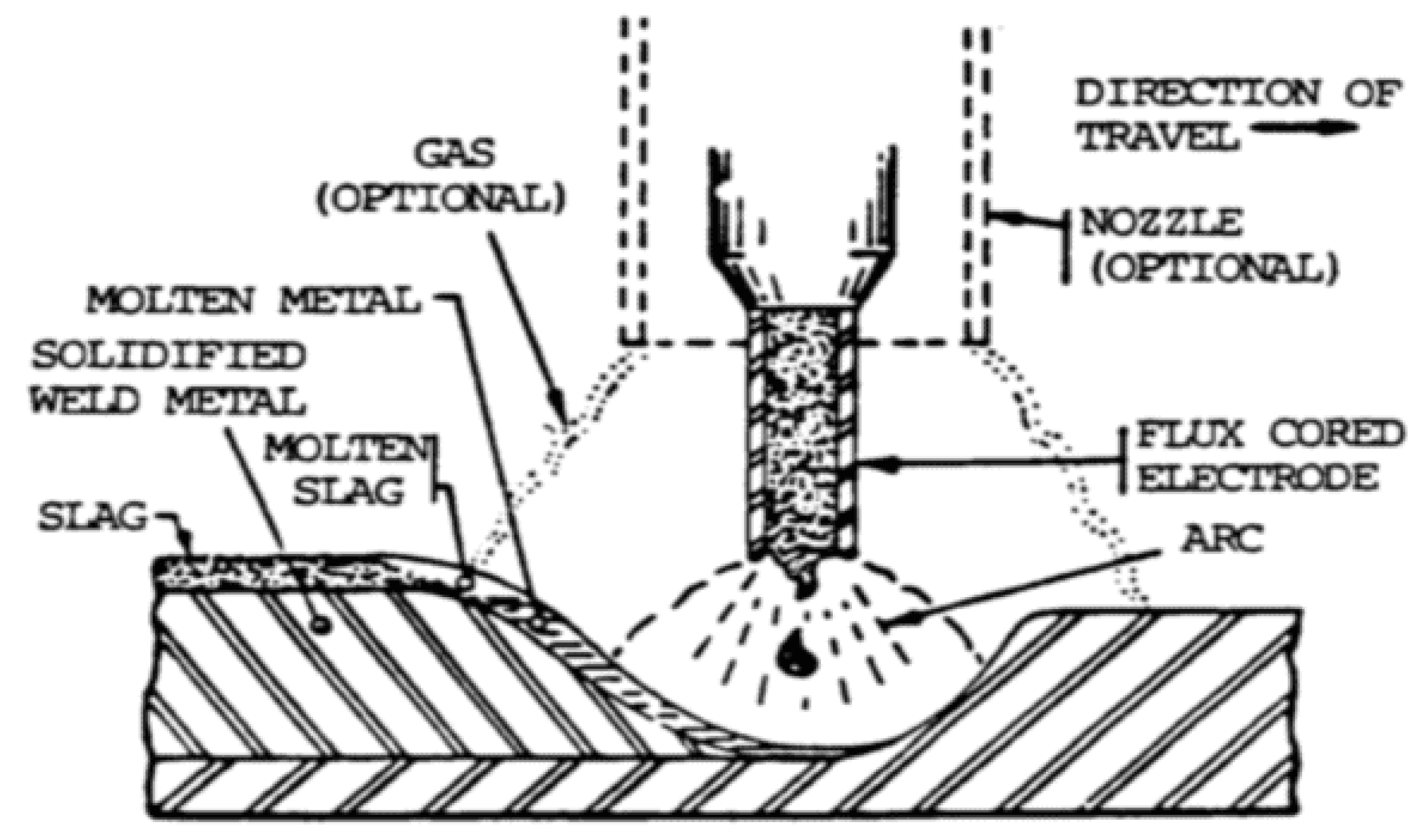
Figure 2.
Scheme of the GMAW welding process. Source [4].
Figure 2.
Scheme of the GMAW welding process. Source [4].
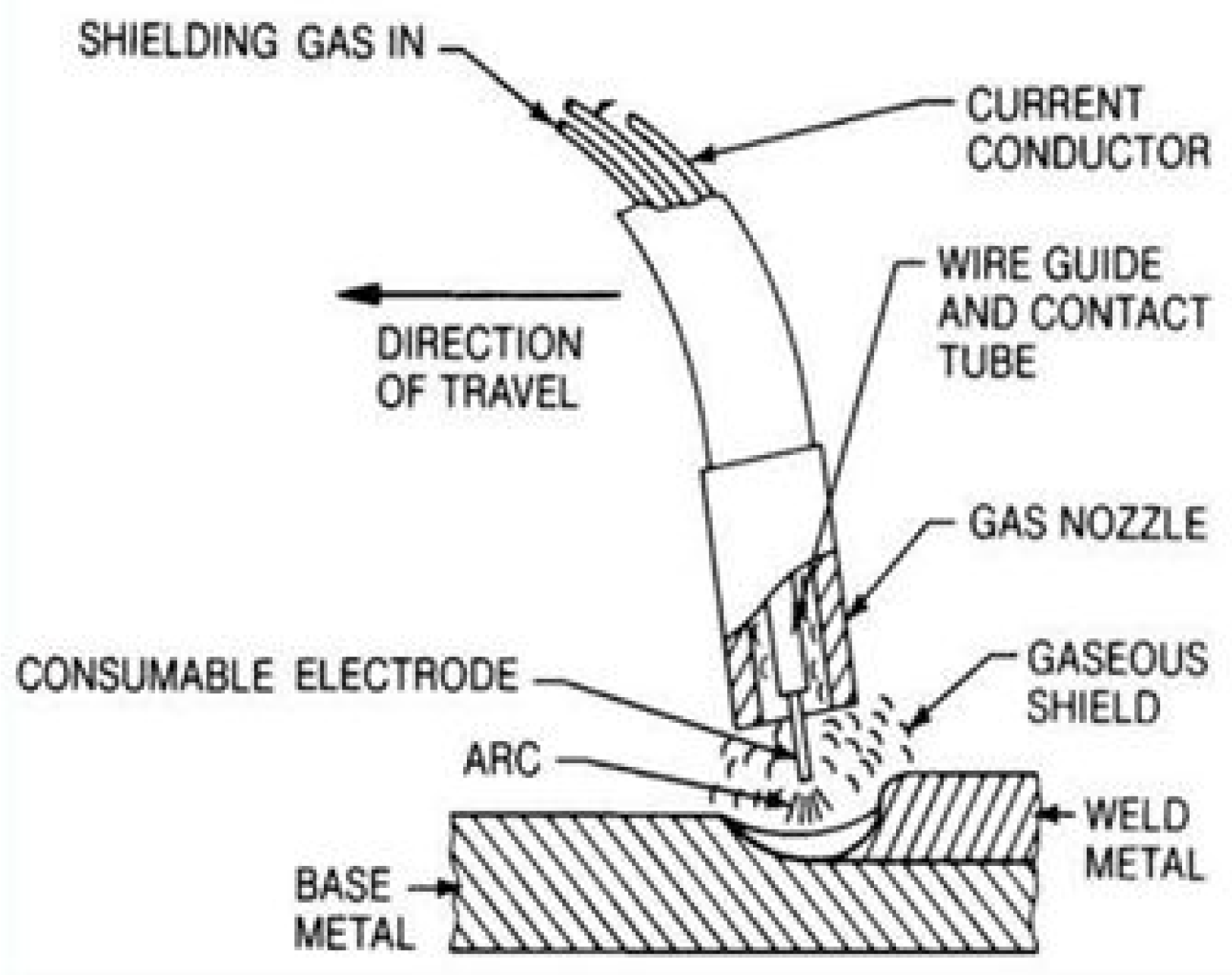
Figure 3.
On the left side, Fanuc 200i-D 7L robotic arm equipped with a welding torch. In the background of this image, you can see the gas bottles (Argon/Carbon Dioxide) in their conveniently mixed proportions. On the right side, appears the Lilcoln R450 CE Multi-Process Welding Machine, placed under the table of the robotic arm and connected to it.
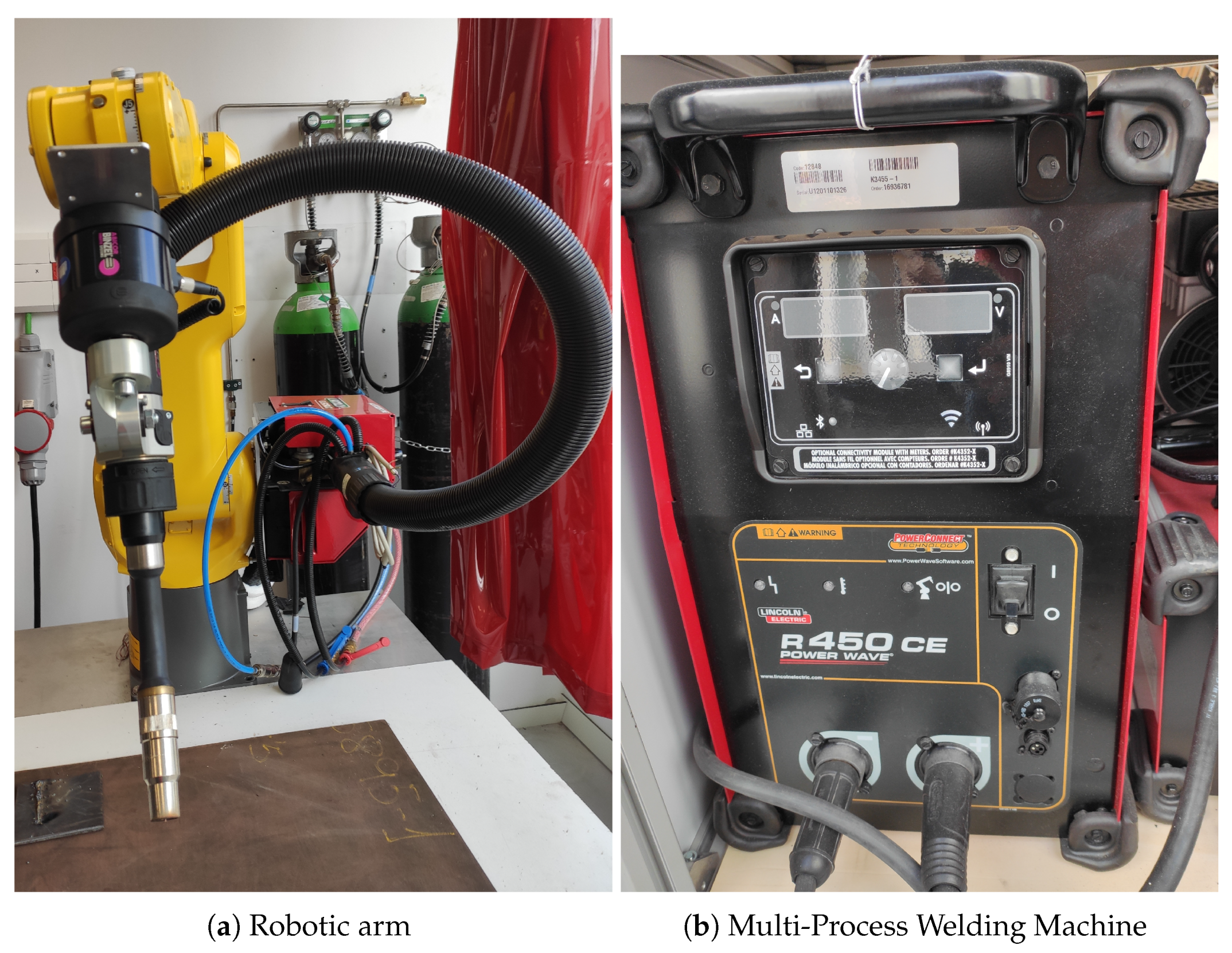
Figure 4.
Steel plate where numbered seams were welded and then treated according to the experiment to be carried out.
Figure 4.
Steel plate where numbered seams were welded and then treated according to the experiment to be carried out.
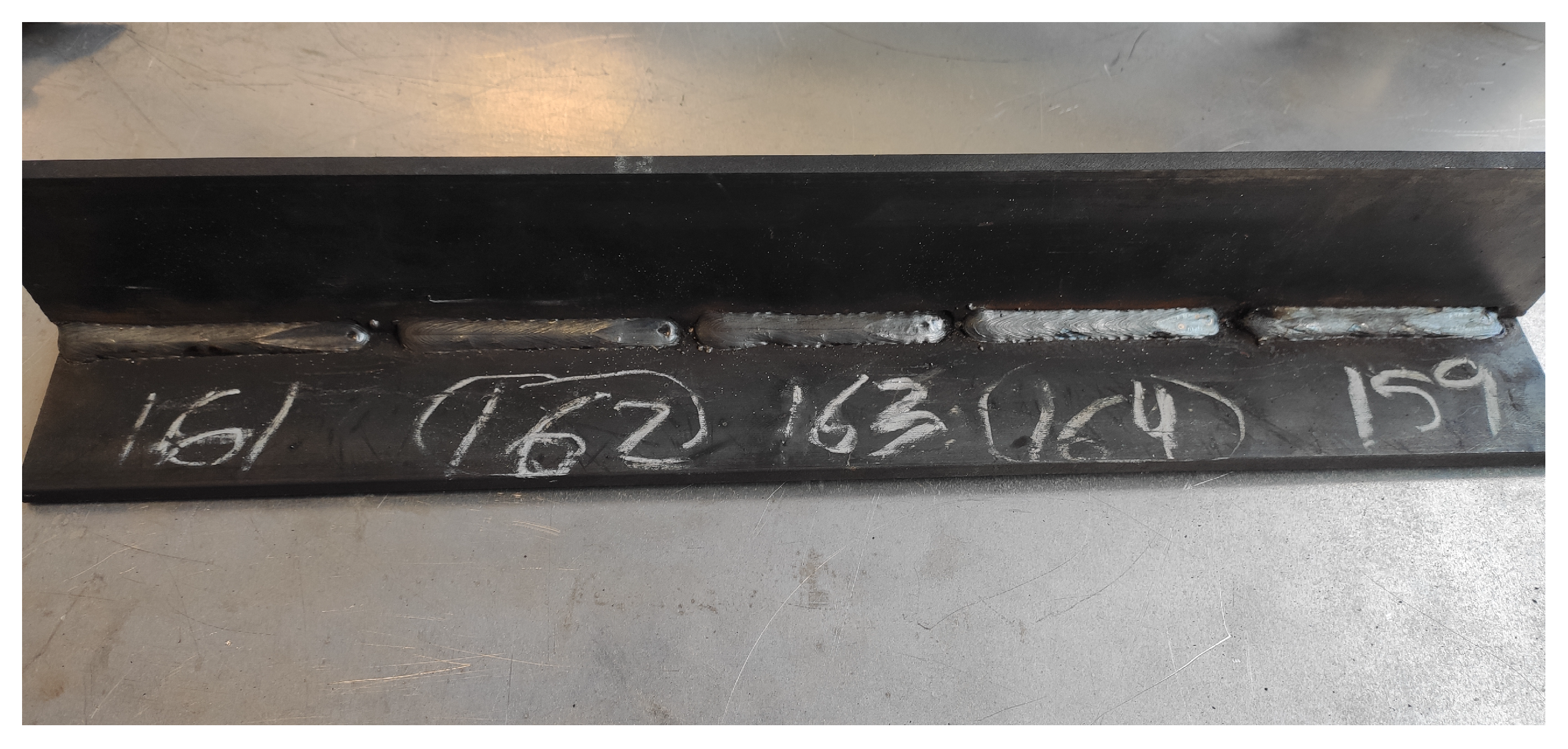
Figure 5.
Equipment used to capture images in different positions and luminosity. The high-precision camera was placed on the end effector of the robotic arm, while the luminaire was placed in different positions, depending on the image being taken. To achieve a series of images with the most varied luminosity possible, for more extensive training.
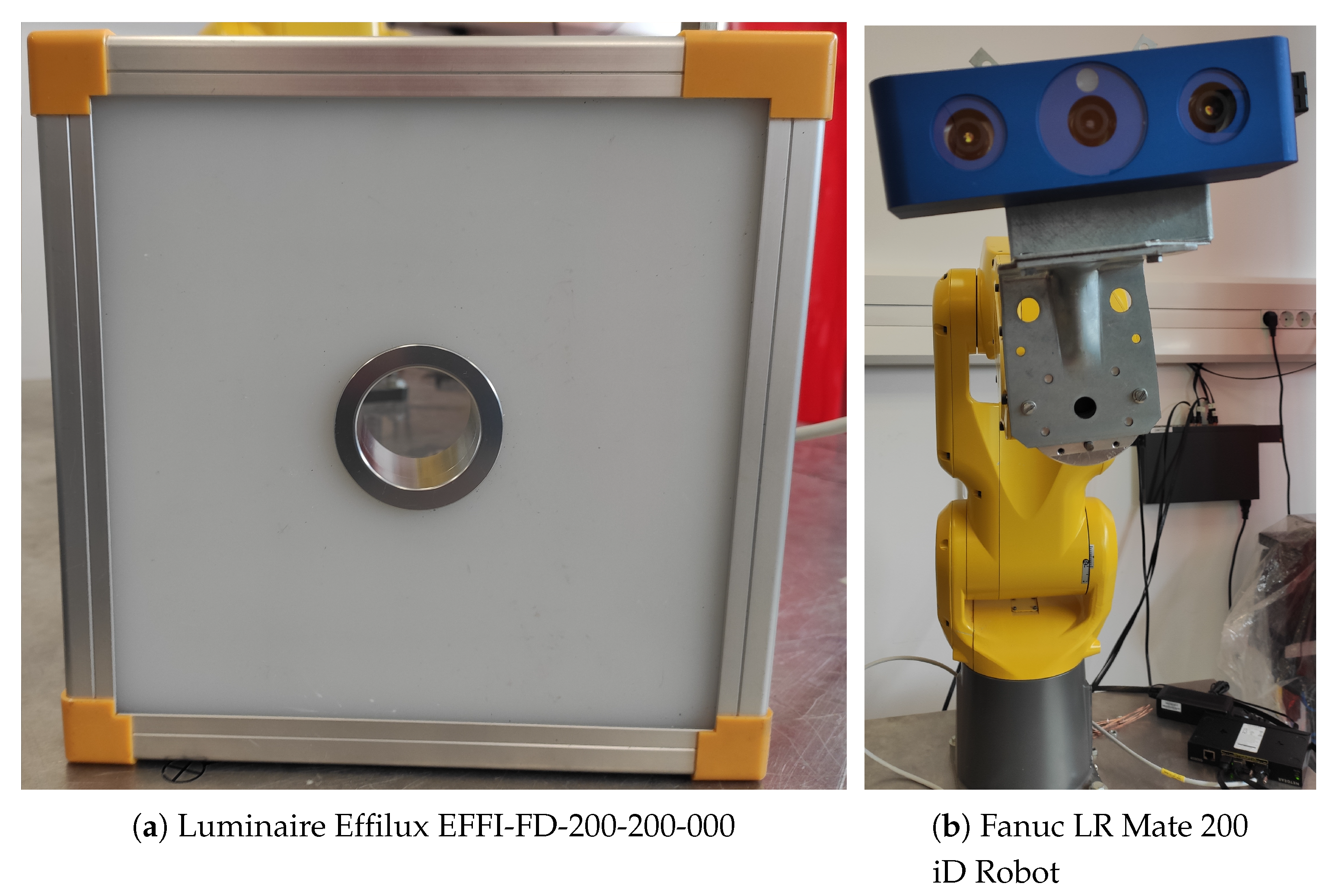
Figure 6.
Diagram of the methodology followed in this work. It begins with the manufacture of the welds necessary for the proposed experiments, and the acquisition of images of these welds. Next, a series of transformations are carried out on these images to finally train three models, one per experiment, that can detect the manufactured weld seams.
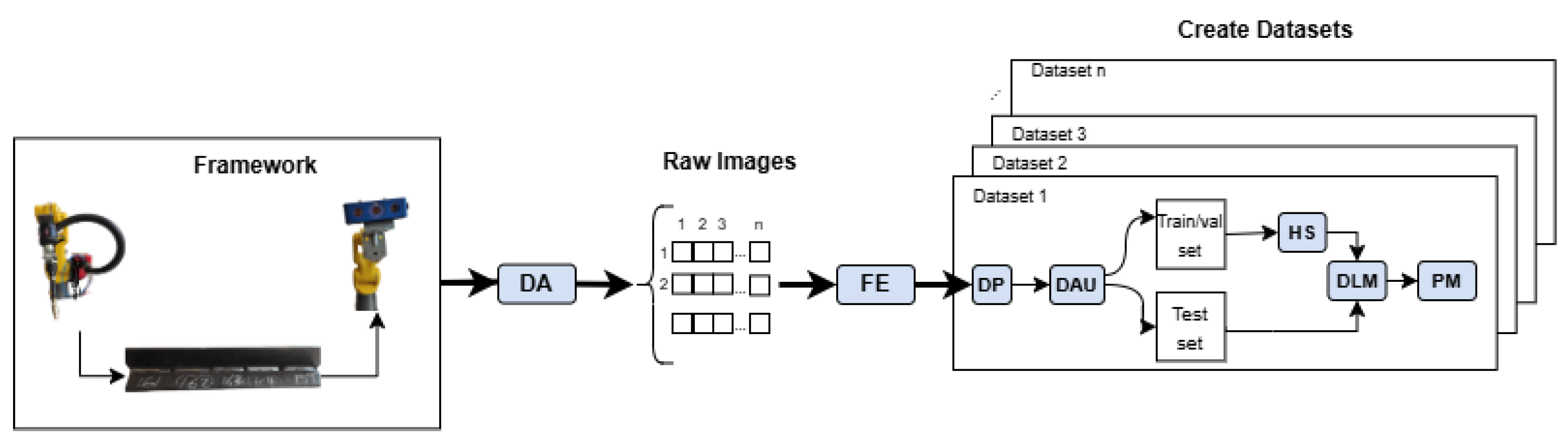
Figure 7.
Industrial camera brand Ensenso model N35 (IDS-IMAGING, Germany), used to take images of weld seams.
Figure 7.
Industrial camera brand Ensenso model N35 (IDS-IMAGING, Germany), used to take images of weld seams.
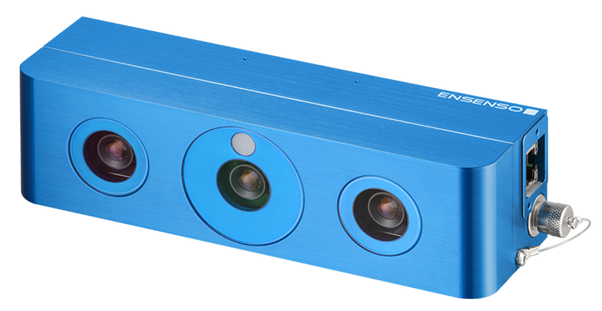
Figure 8.
Mild steel plate with several welding beads, labeled with the online tool Roboflow, so that the system can detect a type of weld manufactured correctly, compared to another weld manufactured with some defect.
Figure 8.
Mild steel plate with several welding beads, labeled with the online tool Roboflow, so that the system can detect a type of weld manufactured correctly, compared to another weld manufactured with some defect.
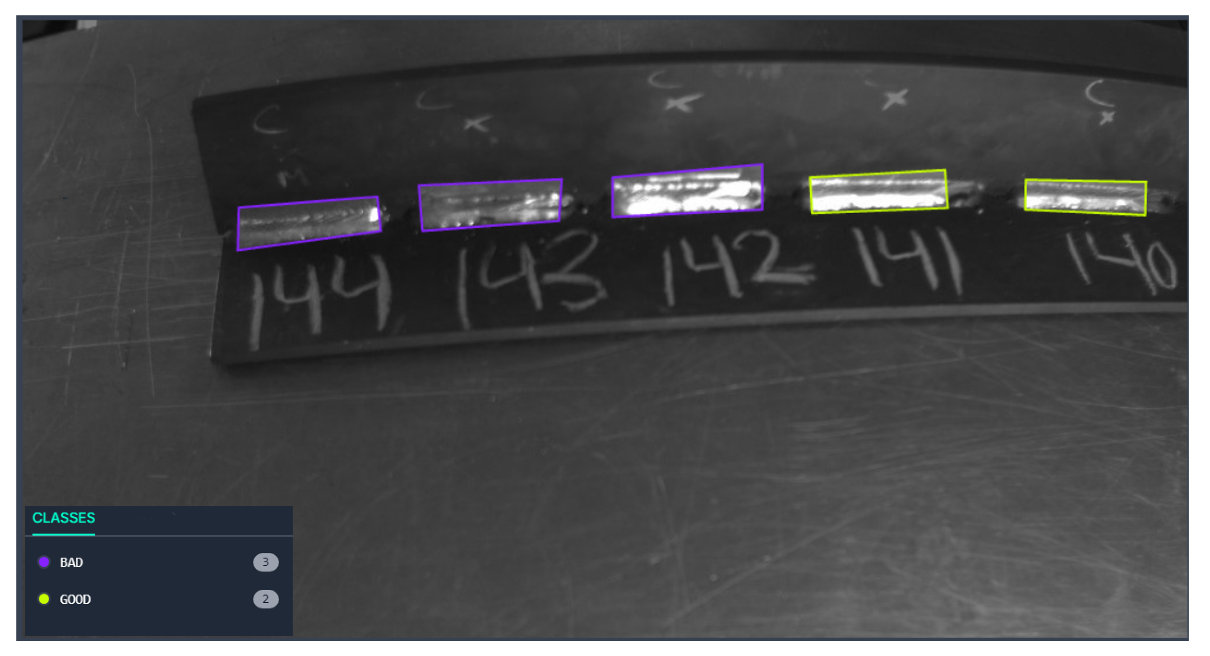
Figure 9.
Set of images of the FCAW-GMAW dataset, where the predicted label and the percentage of that prediction can be observed. An irregular character of the image content can be observed, where the welding bead occupies practically all the space of the image.
Figure 9.
Set of images of the FCAW-GMAW dataset, where the predicted label and the percentage of that prediction can be observed. An irregular character of the image content can be observed, where the welding bead occupies practically all the space of the image.
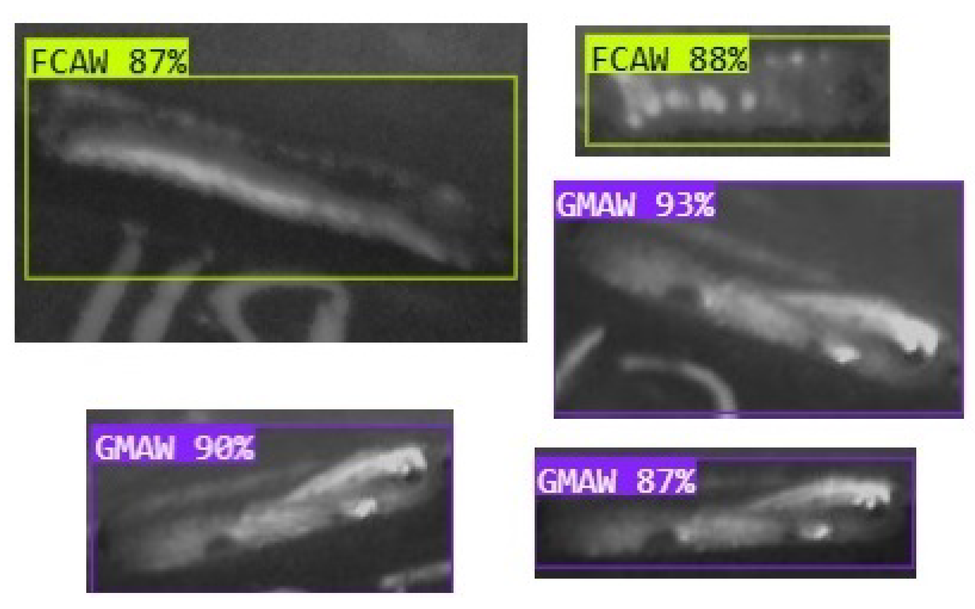
Figure 10.
Training curves and performance metrics for the YOLOv8s object detection model trying to detect FCAW and GMAW weld seams. In all of them we have the training epochs on the x-axis, while the y-axis represents the loss values, both without units. The curves show the learning of the model, observing a significant decrease in the loss, while at the same time improving the precision, recall and mAP50 scores, which leads us to think that the training has been effective.
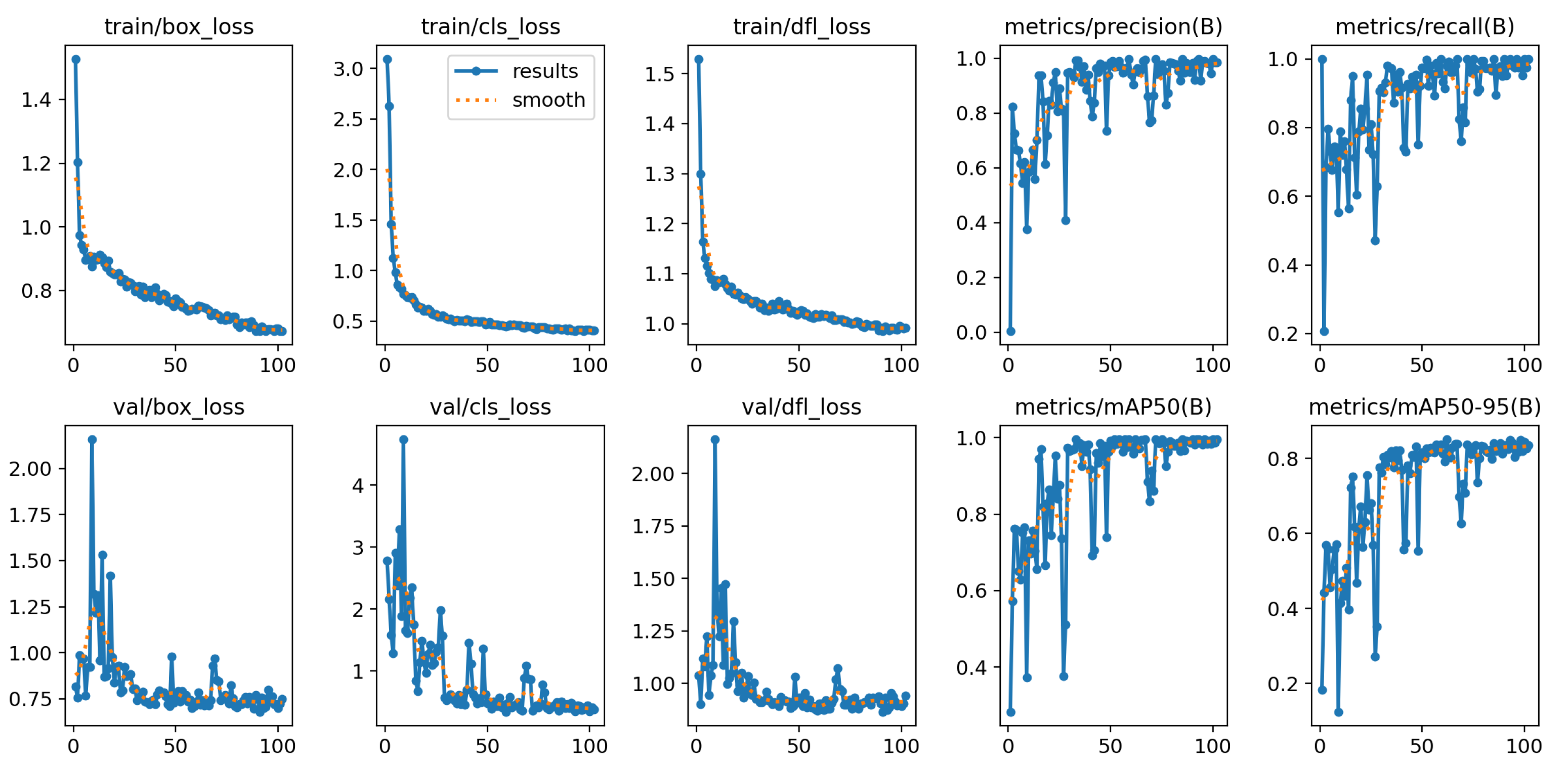
Figure 11.
Plate of fillet weld beads where different beads can be seen, some labeled as GOOD and others as BAD, according to what the algorithm has learned once trained.
Figure 11.
Plate of fillet weld beads where different beads can be seen, some labeled as GOOD and others as BAD, according to what the algorithm has learned once trained.
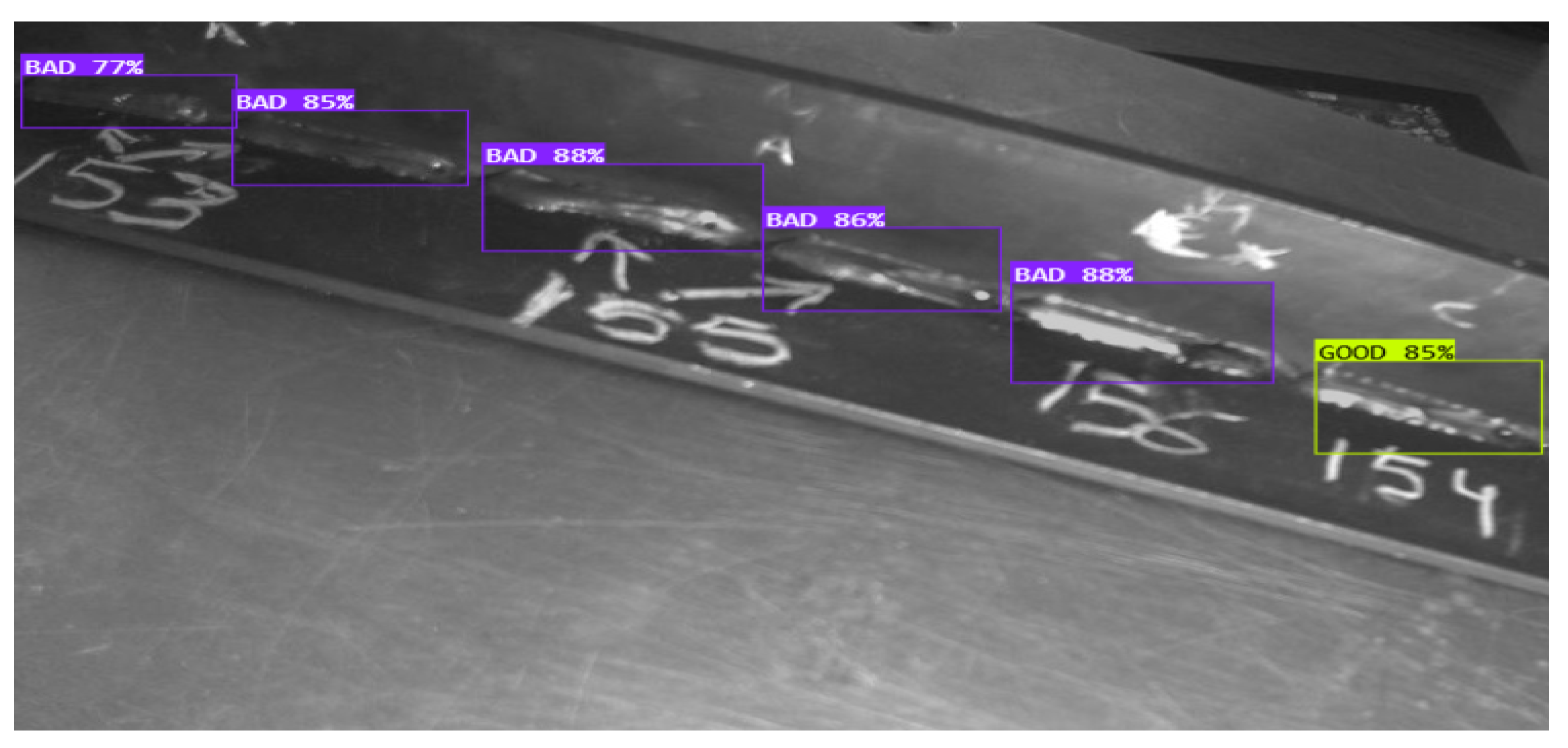
Figure 12.
Training curves and performance metrics for the YOLOv8s object detection model trying to detect weld seams manufactured without defects (labeled as GOOD) and weld seams with some manufacturing defects (labeled as BAD). The x-axis shows the training epochs, while the y-axis shows the loss values, both without units. The curves show the learning of the model, observing a significant decrease in loss, while the precision, recall and mAP50 scores improve, which leads us to think that the training has been effective.

Figure 13.
Plate of fillet weld beads analysed with the model obtained in experiment 3. It shows three of the four types of weld beads (objects) for which the model of this experiment has been trained. In addition, the image shows other elements that the model is able to discard.
Figure 13.
Plate of fillet weld beads analysed with the model obtained in experiment 3. It shows three of the four types of weld beads (objects) for which the model of this experiment has been trained. In addition, the image shows other elements that the model is able to discard.
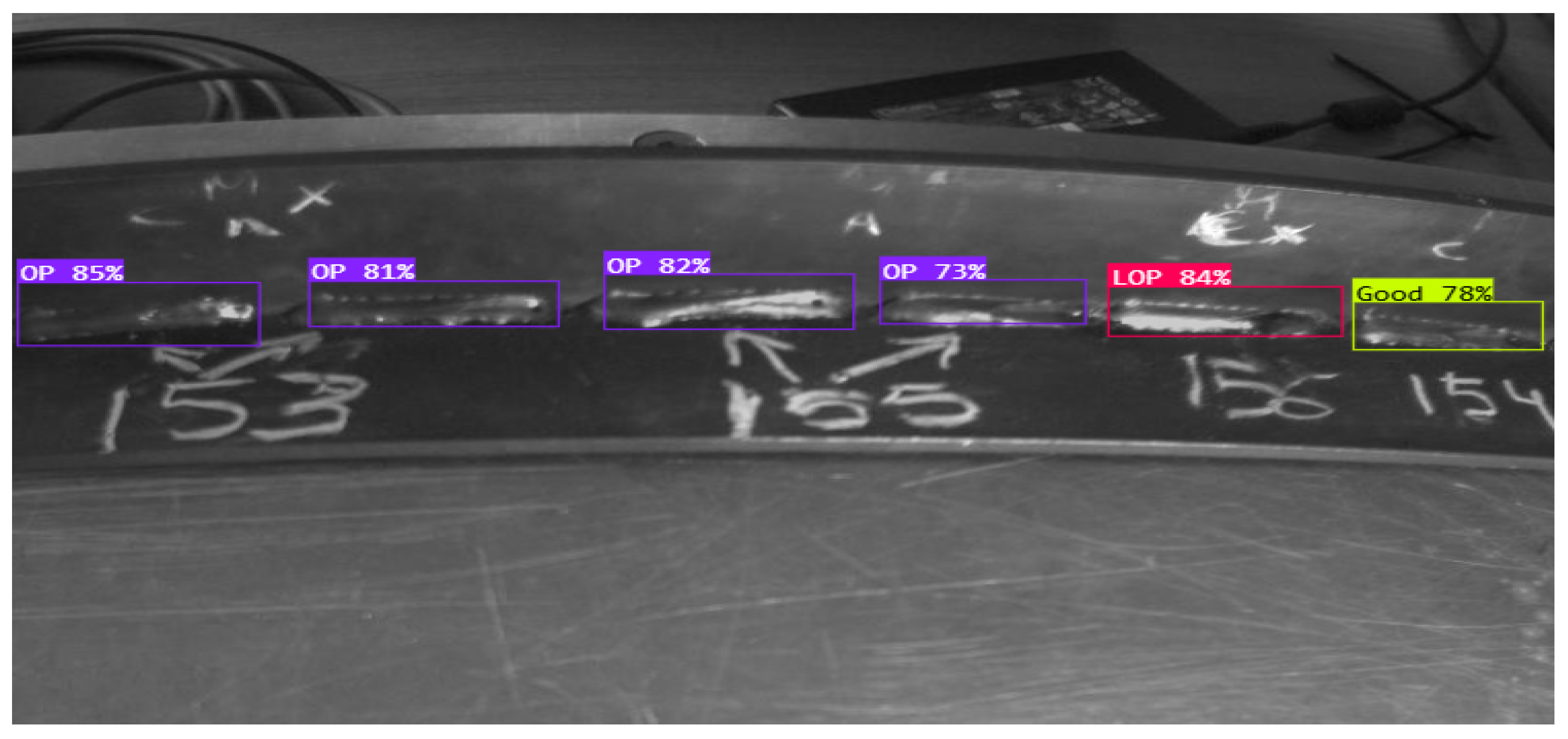
Figure 14.
Training curves and performance metrics for the YOLOv8s object detection model where we try to detect correctly manufactured weld seams, without any defects (labeled as GOOD) and weld seams with some manufacturing defect, labeling and classifying several of these most common defects (labeled as UNDER for Undercuts, LOP for Lack Of Penetration, and OP for Other problems). The x-axis shows the training epochs, while the y-axis shows the loss values, both without units. The curves show the learning of the model, it is observed that the loss is significant although somewhat milder than in the two previous experiments. Same case as in the precision, recall and mAP50 scores that although lower than before, we can deduce that the training has been effective.
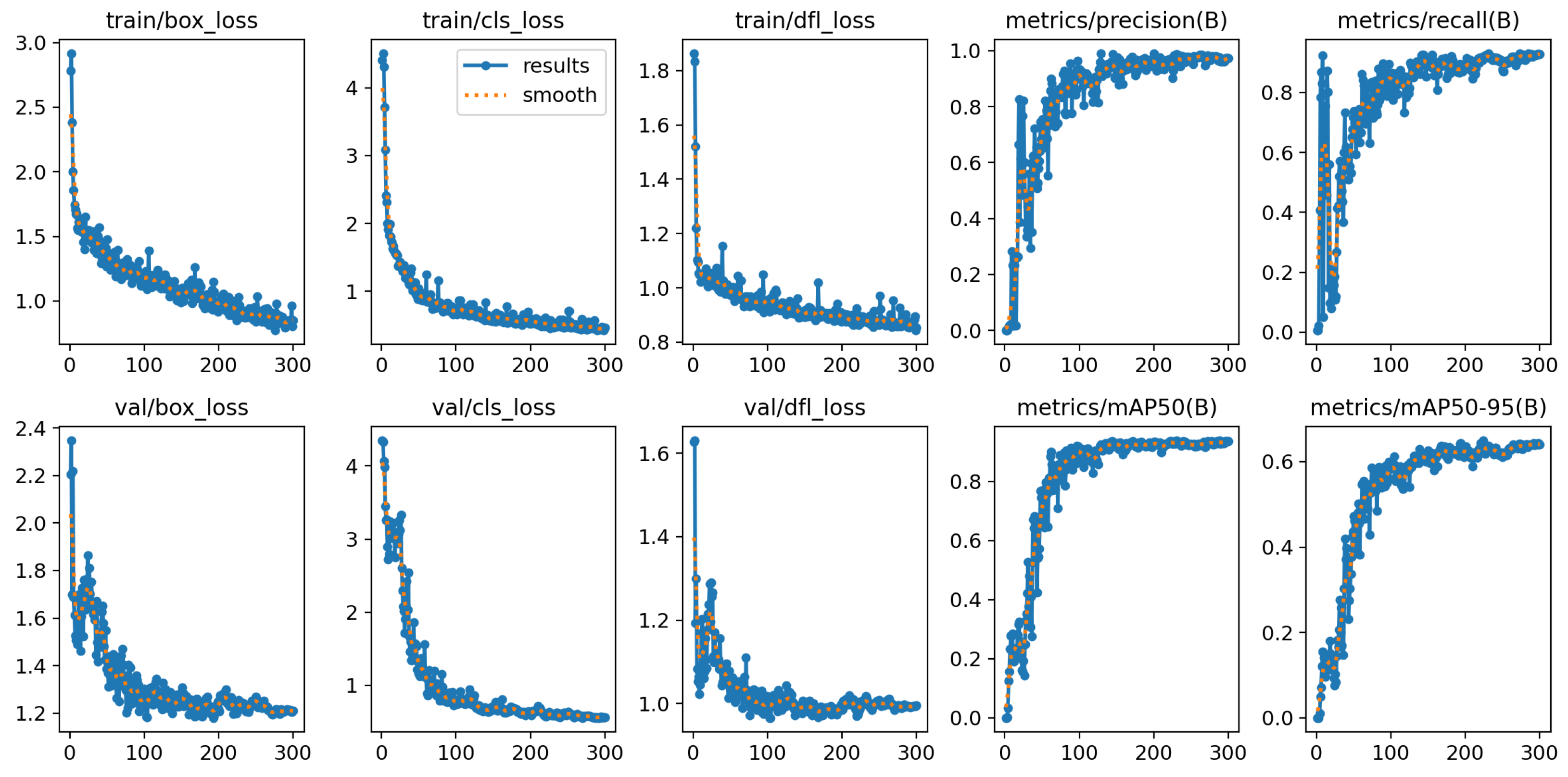

Table 1.
Hyperparameters used in each of the experiments performed.
| Parameter | Experiment 1 | Experiment 2 | Experiment 3 |
|---|---|---|---|
| epochs | 105 | 300 | 300 |
| batch size | 16 | 16 | 16 |
| Learning rate | 0.01 | 0.01 | 0.01 |
| Optimizer | SGD | SGD | SGD |
| Input image size | 320X320 | 320X320 | 320X320 |
| Confidence Threshold | 0.75 | 0.75 | 0.75 |
Table 2.
Performance of the experiments performed in this study: Precision, Recall, and mAP. The latter taken on the validation set and on the training set.
Table 2.
Performance of the experiments performed in this study: Precision, Recall, and mAP. The latter taken on the validation set and on the training set.
| Experiment | Class | Precision | Recall | mAP Val. set |
mAP Test set |
|---|---|---|---|---|---|
| FCAW-GMAW weld seam | FCAW | 0.951 | 0.979 | 0.99 | 0.99 |
| GMAW | 0.99 | 0.97 | |||
| GOOD-BAD weld seam | GOOD | 0.982 | 0.985 | 0.99 | 0.93 |
| BAD | 0.99 | 0.99 | |||
| GOOD-LOP-UNDER-OP weld seam | GOOD | 0.965 | 0.92 | 0.99 | 0.99 |
| LOP | 0.77 | 0.94 | |||
| UNDER | 0.99 | 0.92 | |||
| OP | 0.99 | 0.99 |
Disclaimer/Publisher’s Note: The statements, opinions and data contained in all publications are solely those of the individual author(s) and contributor(s) and not of MDPI and/or the editor(s). MDPI and/or the editor(s) disclaim responsibility for any injury to people or property resulting from any ideas, methods, instructions or products referred to in the content. |
© 2024 by the authors. Licensee MDPI, Basel, Switzerland. This article is an open access article distributed under the terms and conditions of the Creative Commons Attribution (CC BY) license (http://creativecommons.org/licenses/by/4.0/).
Copyright: This open access article is published under a Creative Commons CC BY 4.0 license, which permit the free download, distribution, and reuse, provided that the author and preprint are cited in any reuse.


