2. Interval Values and Operations
Interval calculations in mathematics have been known for a long time, see for example [
7]. In our case, this theory is used at the level of definitions and properties of some interval operations. We will consider the set of values of the time interval as a segment of integers on the number line with starting and end points included.
Definition 1.
Let be a finite set of natural numbers from one to with zero added. Everywhere below, by an interval or domain , unless otherwise stated, we denote the closed bounded subset N of the form
The set of all intervals is denoted by
. We will write the elements of
in capital letters. If
, then we will denote its left and right end points as
and
. We will call the elements of
interval numbers. Two intervals
A and
B are equal if and only if
and
. According to the total interval approach [
7], we can describe operations as follows. Let ∘ be some operation and
. In this case, we have
If
and
, then
We will use only two interval operations: ”+” and ”max”. They are defined as follows:
To illustrate, consider the following example.
Example 1.
Let and . Then
If and , then
While in the first case, the interval A is obtained by the operation max, in the second case a subinterval of B results.
To illustrate, below are some further examples of various options for interval intersection.
A confluent interval, i.e., an interval with coinciding end points , is identical to the integer a. Thus, . If A and B are confluent intervals, then the results of the operations on intervals coincide with ordinary arithmetic operations for positive integers. An interval integer is a generalization of an integer, and the interval integer arithmetic is a generalization of the integer arithmetic.
Note also that for
, we write for simplicity also
. In the theory of intervals, the role of zero is played by the usual 0, which is identified with the confluent interval [0, 0]. In other words,
Calculations can lead to an interval
if
, which, according to Definition
1, represents an empty set.
3. Solving the Permutation Flow Shop Equivalence Problem
Consider the description of the PFSP [
8]. Let
be the set of jobs and
be the set of machines arranged sequentially. Moreover, let
be the processing time of job
j on machine
k.
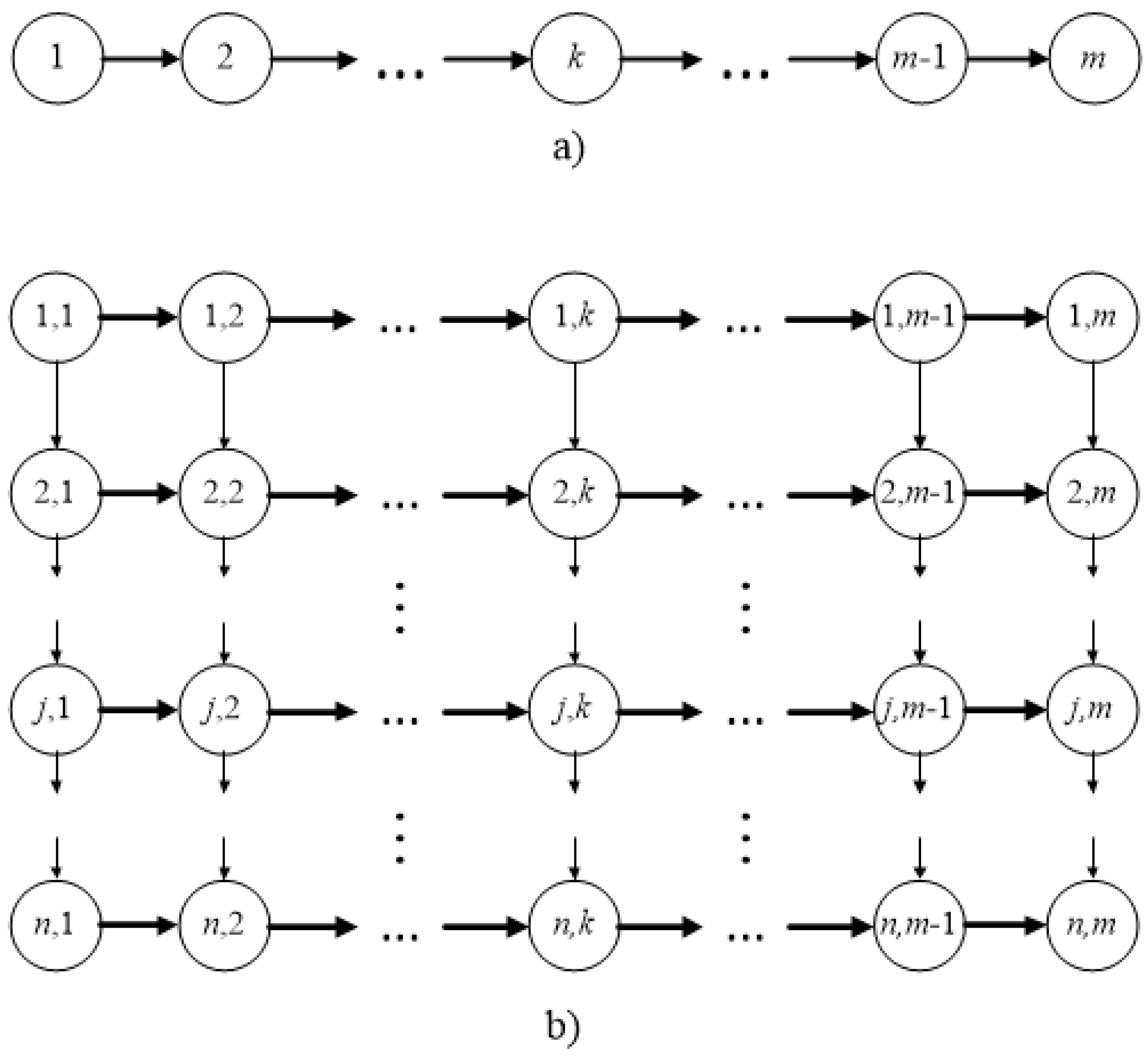
The precedence graph of such a problem (see
Figure 1a) is a simple chain in which the vertices are machines, and the edges define precedence relations between the machines. This graph can be ”expanded” if we fix some order of the jobs and define precedence relations between the jobs
and between the machines
. Any vertex of such a graph is identified with the pair (job number, machine number). An expanded graph describing precedence relations between the jobs is presented in
Figure 1b.
The vertical edges define precedence relations between the jobs for a particular machine. The horizontal edges define precedence relations between the machines for a fixed job. This graph is acyclic and has one start and one end vertex. Consider some schedule and then renumber the jobs in the order in which they are located in the schedule, i.e., for simplicity of the description consider the schedule with the new numbering. The following assumptions are valid for problem PFSP:
Job assumptions: A job cannot be processed by more than one machine at a time; each job must be processed in accordance with the machine precedence relationship; the job is processed as early as possible, depending on the order of the machines; all jobs are equally important, meaning there are no priorities, deadlines or urgent orders.
Machine assumptions: no machine can process more than one job at a time; after starting a job, it must be completed without interruption; there is only one machine of each type; no job is processed more than once by any machine.
Assumptions about the processing times: the processing time of each job on each machine does not depend on the sequence in which the jobs are processed; the processing time of each job on each machine is specific and integer; the transport time between machines and a setup time, if any, are included in the processing time.
Additional time limits can be set in the scheduling problems. Denote
as the interval completion time of job
j by the
kth machine.
is the minimal time for the completion of job
j on the
kth machine, and
is the corresponding maximal time. The completion time
must satisfy the condition
, otherwise the schedule is infeasible. In fact, this is the interval function completion times of job
j on machine
k. We will assume that in the initial formulation of the problem, a matrix
of initial domains of the feasible values for the job completion times has been defined. We will assume, unless otherwise specified, that the initial domains are the interval
, where
is a sufficiently large finite value which will be discussed below. We describe two additional restrictions [
8]:
is the moment when job j arrives for processing, i.e., its release date. This parameter defines the point in time from which job j can be scheduled for execution, but its processing does not necessarily begin at this moment. In this case, in the matrix of initial domains, it is necessary to put for and .
is the deadline for processing job j. A deadline cannot be violated, and any schedule that contains a job that finishes after its deadline is infeasible. In this case, in the matrix of initial domains, it is necessary to put for and .
The combination of the constraints
and
generates initial domains of the form
for
and
. If these restrictions relate to specific operations, they will look like
and
. In this case, the following time relations will be satisfied:
Here we take into account the fact that the interval time
for the start of job
j on the
kth machine is calculated by the formula
The above inequalities are supplemented by inequalities of the form .
The system of inequalities (
2)-(5) defines an infinite set of feasible schedules. To reduce this set to a finite one, we will use a positive integer constant
and supplement the system (
2)-(5) with the inequalities
It is possible to assign to
a value so small that the set of feasible schedules is empty. We assume that the value of
is such that there is at least one feasible schedule.
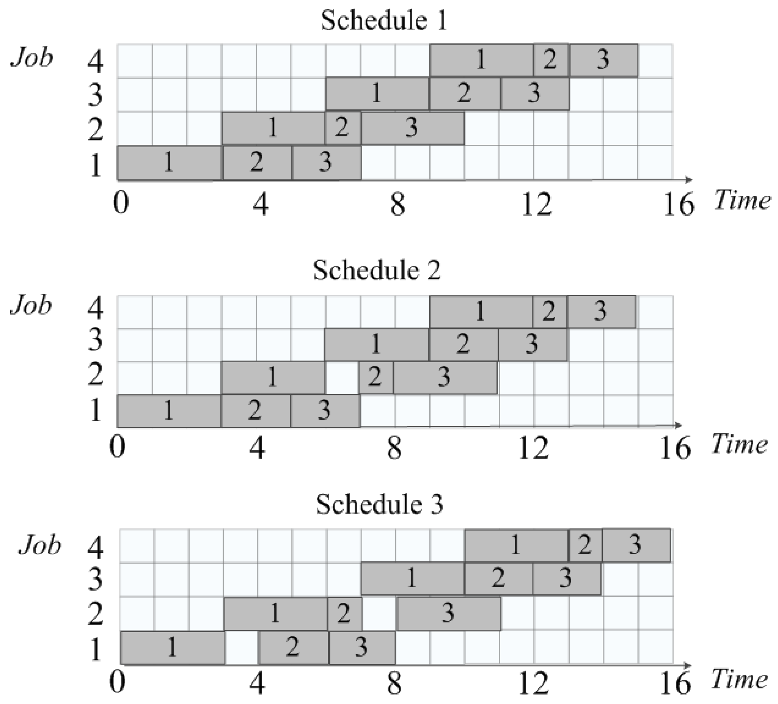
Example 2. Consider a PFSP with 3 machines and 4 jobs.
Table 1 shows the processing times of the jobs. The rows correspond to the job numbers, and the columns represent the machine numbers.
Let . In this case, the intervals for each pair are given in Table 2.
Figure 2 shows the Gantt charts of three variants from the set of feasible schedules. ”Schedule 1” and ”Schedule 2” are optimal schedules (for this sequence), while ”Schedule 2” and ”Schedule 3” have different inserted idle times. It is easy to verify that increasing any interval in Table 2 will lead to the appearance of infeasible schedules, and decreasing any interval will result in the loss of feasible schedules.
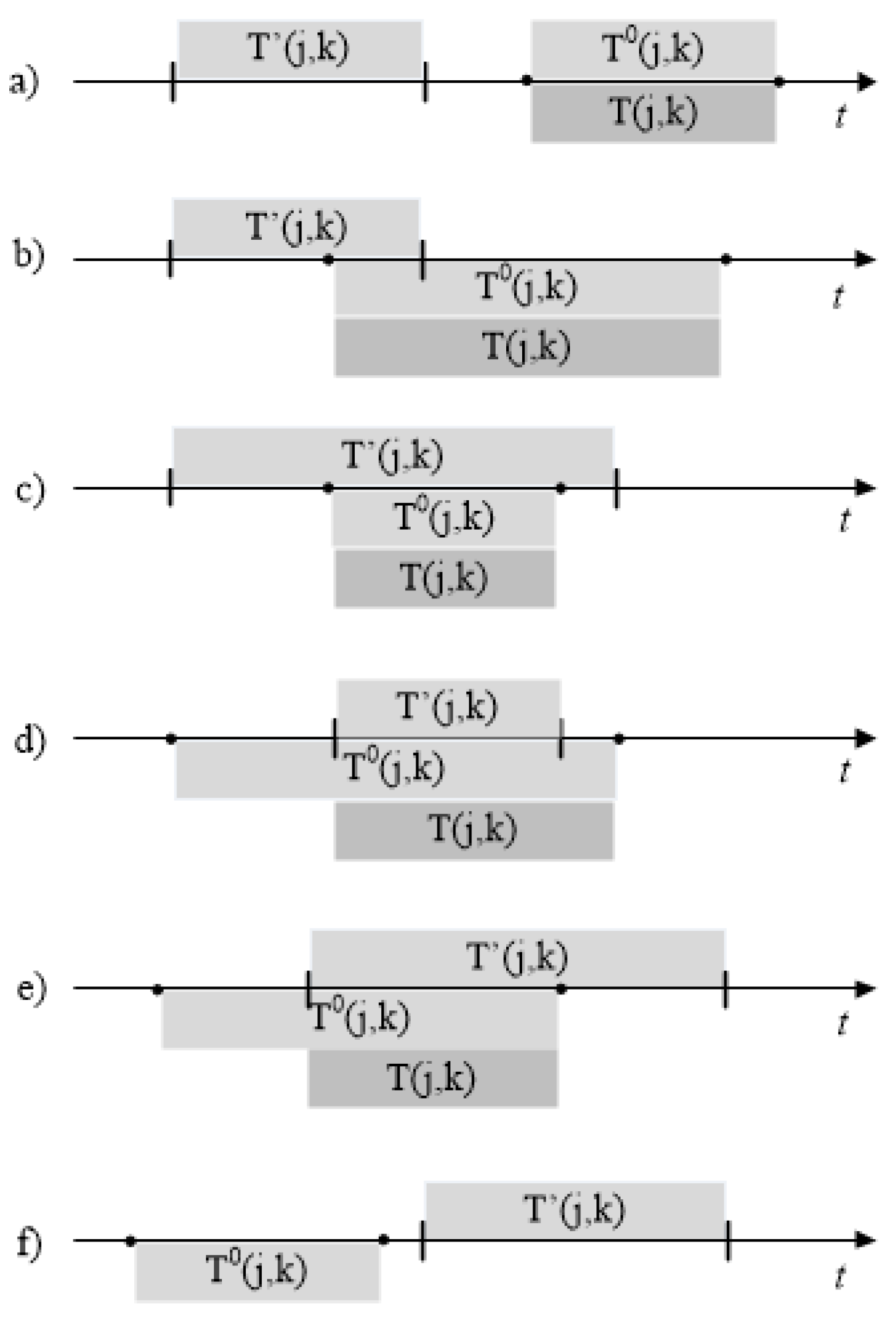
Let
be the interval calculated by some algorithm for completing the
jth job on the
kth machine and
be the corresponding initial domain. According to
Figure 3, we define the interval noncommutative operation intersection (∩) as
. The figure shows all significant cases of interval intersections:
- a)
the interval is to the left of . The completion time of the jth job on the kth machine should be artificially increased to values from the interval . Only in this case, the schedule wil be feasible;
- b-e)
are cear without additional explanation;
- f)
with this arrangement of intervals, the value of the interval is equal to an empty set, which corresponds to the absence of a feasible schedule.
It can be shown that all feasible sets of time values are uniquely determinable and maximal. Therefore, when searching for an optimal solution, no solution will be lost.
All precedence relations define intervals (including the scalar ). Again for simplicity of the description, consider some schedule and then renumber the jobs in the order in which they are located in the schedule, i.e., consider then the schedule with the new numbering. The calculations of these intervals can be divided into 4 groups. Next, we write them using interval variables, assuming that the initial interval is and :
For the completion of the 1st job on the 1st machine
, we have:
For the completion of the 1st job on the
kth machine
, we have:
For the completion of the job
j on the 1st machine
, we have:
The interval of the completion time of job
j on the
kth machine
is obtained as follows:
The PFSP can be formulated using a finite set of special recursive functions. This is due to the existence of precedence relationships between the machines and jobs in the PFSP when the current characteristics of the problem are determined by the preceding ones. Recursive functions have arguments and parameters as data. The arguments of the functions are pairs (job number, machine number). They are passed as function arguments in the normal mathematical sense. Parameters are defined outside the recursive function, and they are essentially global variables in imperative programming terms. Examples of parameters can be: , and so on. The calculated value (or set of values) of the function is the completion time of job j on the kth machine.
We will denote the interval recursive function as . Specific types of recursive functions will be provided subsequently as the PFSP is considered. Let us consider the problem of equivalence of the existing PFSP formulation in the literature and its recursive representation. The equivalence of both formulations is established through the equivalence of the domains of acceptable values of the completion times for each pairs (job number, machine number). An optimal solution is within the allowed processing times. This fact allows us to move to the functional representation of the problem and to apply various appropriate methods. We can describe each group by the corresponding recursive functions:
This set of functions can be combined into one function:
The function
is defined for all values of
j and
k. If
, then there is no feasible schedule. It can be seen from the formula that it calculates the only value of the interval. We show that this recursive function defines the same domain for each
as the set of values defined by the system of inequalities (
2)-(
6).
Theorem 1. Let the following conditions be satisfied for both the PFSP given by the system of inequalities (2)-(6) and the recursive PFSP:
one graph is set for both problems (see Figure 1a); consider some schedule and then renumber the jobs in the order in which they are located in the schedule, i.e., consider the schedule with the new numbering;
the processing time of job j on the kth machine is ;
the same matrix of initial time intervals is specified:
Then the following statement is true: the set of domains (domain of definition) of feasible times for the non-recursive PFSP coincides with the set of domains for the recursive PFSP, i.e., for .
In other words, the sets of valid schedules for each pair (job number, machine number) are the same, or in both cases there is no feasible schedule, i.e., there are j and k such that .
Proof. Let the conditions of the theorem be satisfied. The proof is done by complete induction. Let us recall the formulation of the principle of complete induction. Let there be a sequence of statements
. If for any natural
i the fact that all
are true also implies that
is true, then all statements in this sequence are true. So for
we have
Here
denotes a logical implication. The statement
is the equality of the intervals
. Let us apply this method to the graph in
Figure 1b. From graph theory, it is known that the vertices of an acyclic graph are strictly partially ordered. There exist algorithms for constructing some linear order for a strictly partially ordered graph. Informally, a linear order is when all the vertices of a graph are arranged in a line, and all edges are directed from left to right. Any such algorithm is suitable because:
- the first vertex is always of the original graph,,
- the last vertex is always ,
- when evaluating the recursive function according to a linear order, its arguments have already been evaluated.
Let us choose a row-by-row traversal. In this case, for a pair , all pairs with or have already been considered. We will traverse the elements of the matrix of interval variables T in the rows from left to right and from the top row to the bottom one.
Let us prove the statement
. From the system of inequalities (
2)-(5), it follows that
From the definition of the recursive function, it follows that
Therefore, we have
.
Let us assume that the statements are true. We now prove that he statement is also true. Among the 4 groups of relationship types described above, the first type is considered for .
-
Let us analyze the remaining 3 types.
- 3a)
-
Processing of the 1st job on the kth machine :
In this case, the problem satisfies the equality
In turn,
and due to the condition
, we get
Therefore, we have
.
- 3b)
Processing of job
j on the 1st machine
: In this case, the problem satisfies the equality
In case of recursion,
Due to the condition
, finally we get
Therefore, we have
.
- 3c)
Processing of job
j on the
kth machine
assumes that the problem satisfies the equalities
In this case,
Therefore, we have
.
All possible situations have been analyzed.
□
The main optimization problem in the PFSP is to find the order of job processing so that for some selected criterion, the function value is optimal. The most common criterion is the makespan (i.e., the total time it takes to complete the whole set of jobs). We remind that the vast majority of flow shop problems are treated as a PFSP, see for example [
9,
10,
11].
To effectively solve the problem of calculating an optimal schedule, it is necessary to switch from interval recursive functions (
8) to scalar recursive functions
. Consider the case when all elements of the matrix of initial time intervals are equal to
. In this case, all the cases of interval intersections shown in
Figure 3 will be reduced to case d and will look like in
Figure 4. The value of
will always be equal to
and the interval value can be replaced by a scalar equal to the lower value of the interval
. Then the recursive function (
8) will look as follows:
or finally
The function
calculates the completion time of job
j on the
kth machine. The scalar function (
10) is obtained from the interval function (
8) by replacing the interval with the lowest value of the interval.
In Example 2 above,
computes only one schedule with minimum completion time, which corresponds to the ”Schedule 1” diagram in
Figure 2.
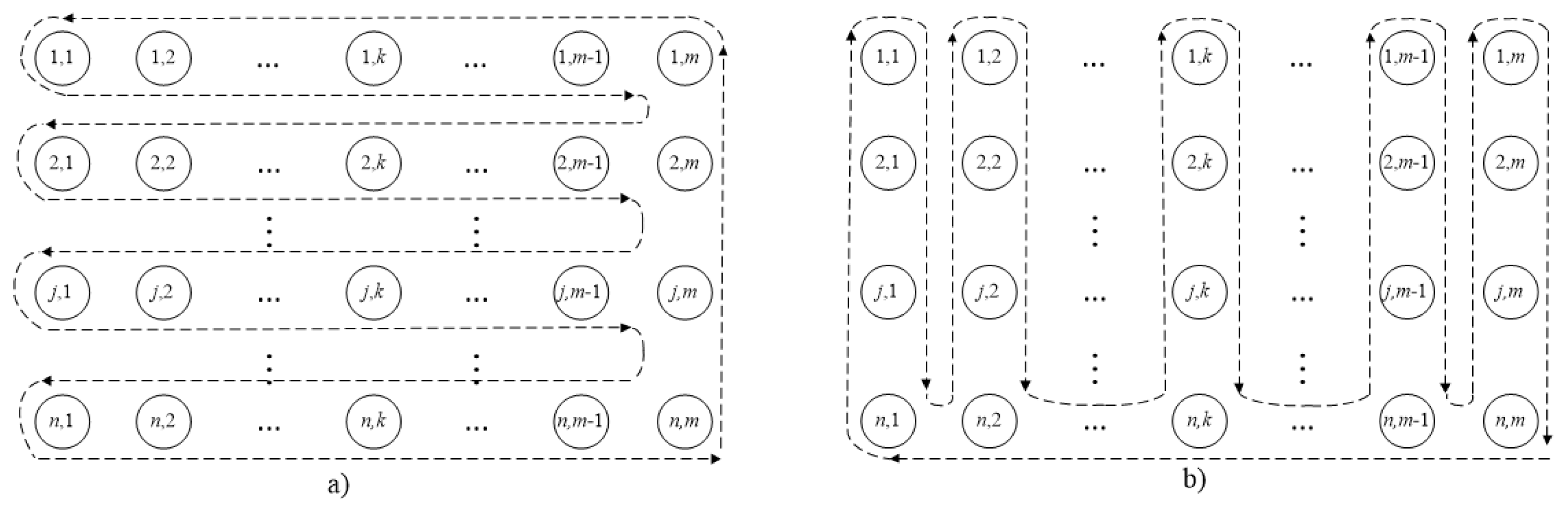
The analysis of formula (
10) shows that when calculating the function
, the traversal of pairs
is carried out in the order indicated in
Figure 5a.
However, if the function (
10) is replaced by an equivalent function (
11) (the difference is in the expression
11d), then the pairs will be traversed according to the scheme in
Figure 5b.
Theorem 2.
Let the PFSP include m machines and n jobs. Consider some schedule and then renumber the jobs in the order in which they are located in the schedule, i.e. consider the schedule with the new numbering. In this case, the following equality is true for any and any :
The point of this theorem is that the scalar function calculates the minimum completion time for any given sequence of jobs. This follows from the principle of the function construction.
Proof. If in the formula (
9)
is replaced by
, then a formula for calculating
is obtained. The direct comparison of the resulting formula with the formula (
10) for calculating
proves the validity of the theorem. □
The following important theorem follows from Theorem 2.
Theorem 3.
Let the PFSP be defined for m machines and n jobs. In addition, let Π be the set of all permutations of n jobs and be the permutation corresponding to the minimum completion time of all jobs, computed as for . For the PFSP, such a permutation satisfies the equality
The meaning of the theorem is that the minimum completion time of all jobs, computed using interval calculations, is equal to the value of the scalar recursive function for the same permutation.
Proof. The set of all permutations is finite and has the cardinality . In this case, as it has been proven by Theorem 2, for any permutation , the equality holds. Therefore, it also holds for the permutation . □
Let us look at Example 2 again. If, after calculating the intervals in
Table 2, we introduce a constraint of the form
(the moment the job is received for processing), this will lead to a change in the intervals for the 3rd job as follows:
, and for the 4th job to
. Among the schedules given in the example in
Figure 2, only ”Schedule 3” will remain feasible. The other schedules will become infeasible. Evaluating the recursive function will not result in a feasible schedule. This example demonstrates the importance of including constraints in the initial value matrix when evaluating the recursive function.
Theorem 3 states that when computing an optimal schedule for the PFSP, one can move from interval calculations to the scalar recursive function
(
10), although the cardinality of the set of values of the function
is less than or equal to the cardinality of the set of values of the function
. If the function
has several minima, then the function
will have the same number of minima.
Denote by the permutation
the order of job numbers, and
, is the number of the job at position
in the schedule (permutation)
. The recursive function was defined before to have a fixed order of the processing of the jobs. Let us add a permutation
to the definition of the function as a global variable so that we can change the order of jobs. We define new functions:
and
. Here
is the set of job position numbers and
. We include the permutation
in the definitions of the recursive functions (
8) and (
10) so that we can change the order of processing the jobs:
In the function , where is the number of the position in the schedule (permutation) and is the number of the machine, are the arguments of the recursive function, and the processing times and the permutation are the parameters of the function.
Example 3. Here we calculate the completion times of the jobs 1 and 2 on the machines 1 and 2. It should be noted that in this case the first argument of the function is the number of the position in the shedule π.
For simplicity of the description, we have discussed the approach for the PFSP. It can be noted that one can extend this procedure to the FSP with possibly different job sequences on the machines:
4. Implementation of the Branch and Bound Method for the PFSP
It should be noted that the PFSP was one of the first combinatorial optimization problems for which the branch and bound (B&B) method was applied [
6] soon after its development [
12]. A large number of works were devoted to the application of the B&B method for solving the PFSP. The papers [
10,
13] review the most important works on B&B algorithms for the PFSP. Since the branch and bound method follows very organically from the recursive representation of the PFSP, we consider it subsequently.
Evaluation of Lower Bound LB1. Taking into account the permutation
of jobs, for a certain pair
, the lower bound LB can be determined as follows:
Remark 1. Calculating the value of the function from the value of the function is simpler than calculating . Therefore, it makes sense to calculate the lower bound only for the pair . In [14], the effectiveness of the comparison with the lower bound on the last machine was also justified.
In this case, it is possible to move from formula (
16) to the formula for calculating the bound on the last machine
Next, let us formulate the exact meaning of the bound
. In the described case, it means that with a fixed order of a part of the jobs
, the processing times of all jobs cannot be less than
for any arrival order of the remaining jobs
.
Let
be the set of permutations of
n jobs for which the value
has already been calculated. Then the lower bound
for the considered job sequences will be
Thus, if the inequality
is satisfied for the current pair
, then this sequence of jobs
is excluded from consideration as not promising, and the corresponding branch of permutations is cut off. The next one will be one of the sequences
with
where
is the set of all permutations of the
remaining jobs.
Branching. First of all, the branching must be consistent with the traversal defined by the recursive function. If
it is necessary to change the order of the jobs. However, it is necessary to change the order in such a way as to minimize the loss of information when calculating the functions
The literature describes many permutation algorithms with different characteristics. Let
.
assigns to each permutation of the set an element
x, i.e.,
. In this case, the algorithm for generating permutations should calculate them in such a sequence that they satisfy the following recursive property:
This property, after calculating the function , allows one to study all permutations of the ”tail” of the queue of jobs being scheduled and only then track back.
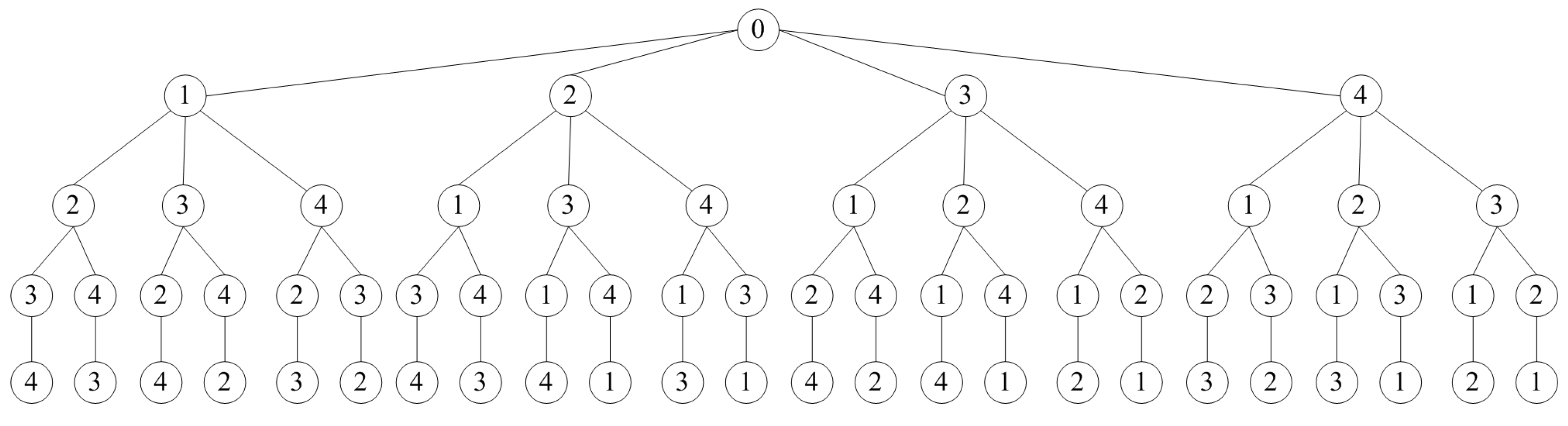
Example 4. Figure 6 shows an example of a complete permutation tree that satisfies Property (18) for . The root of the tree is an auxiliary vertex, and the permutation corresponds to some path from the root. The vertical edge shows the next level of recursion. It connects the initial sequence to its tail. The tree is traversed from top to bottom and from left to right. In this example, the permutations will be generated in the following order: (1,2,3,4),(1,2,4,3),(1,3,2,4),(1,3,4,2),...,(4,3,1,2),(4,3,2,1). There are 24 permutations in total.
This algorithm can be implemented through recursive copying of the tail of permutations. This is a costly operation, but the algorithm can be modified so that the permutation exists in a single instance as a global variable. This is done using forward and reverse permutations of two jobs (when returning along the search tree). The description of the B&B algorithm is given in Appendix A.
5. ”And” Function
The flow shop problem discussed above is more a subject of theoretical research and has limited applicatiosn in practice. In order to bring it closer to practice, various additional elements can be introduced, first of all, various types of constraints. In real production, the main machine chain is served by various preparatory operations, for example: those associated with delivery from the warehouse to the production line; preparatory steps; technological issues; testing, etc.
Next, we expand the PFSP by introducing the
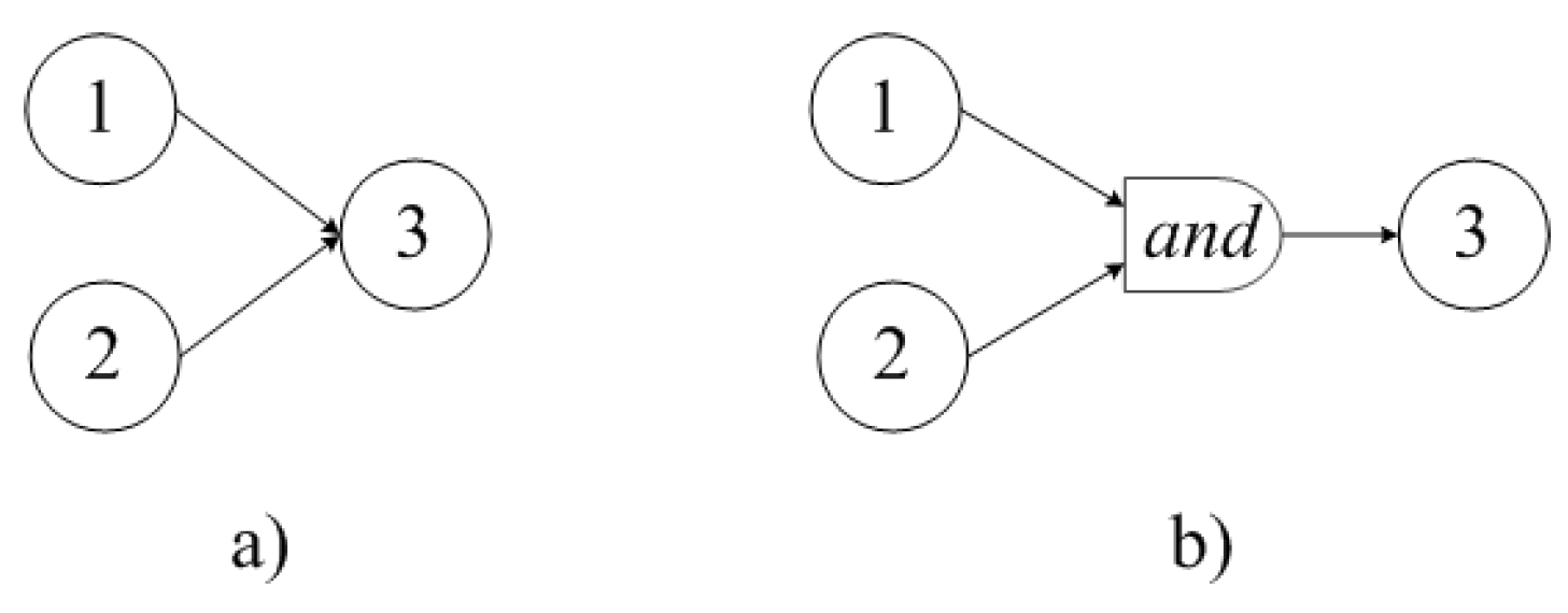
function. A well-known construction, shown in
Figure 7a, denotes a precedence relation in which the execution of a job on machine 3 can only begin after the completion of the jobs on machines 1 and 2. Using the
function, it will look like in
Figure 7b. In what follows, we will interpret the
function as a machine with zero processing time for any job. Thus, the chained precedence graph for the PFSP is expanded into a tree precedence graph when using the
function. Thus, the PFSP is transformed towards an Assembly Line job (AL), but without the presence of a conveyor belt and workstations. This problem can be called the Assembly Permutation Flow Shop problem (APFSP) . The absence of a conveyor belt frees from the ”cycle time” limitation, and the absence of workstations frees from solving the balancing problem, i.e., an optimal distribution of the jobs among the stations, taking into account the cycle time.
Despite the absence of assembly line attributes, this model can have a wide application.
The function
in the interval representation
looks as follows:
or
or in a scalar expression
.
Accordingly, we get the function
, where
is a set of job position numbers and
:
Including the
function into the PFSP causes the machines to process the job according to the precedence tree. To set a specific order of the precedence graph traversal, we assume that the function
is always the first one in the formula (
19) and determines the upper arc in
Figure 7b. Adding the
function causes the assumption in
Section 3 to be invalid: ”a job cannot be processed by more than one machine at a time”, since the machines 1 and 2 in
Figure 7b can execute the same job simultaneously.
It can be proven that when adding the function
to the PFSP (i.e.,
and
), Theorem 3 remains valid, and the function
supplemented by
also implements a greedy algorithm for a fixed sequence of jobs.
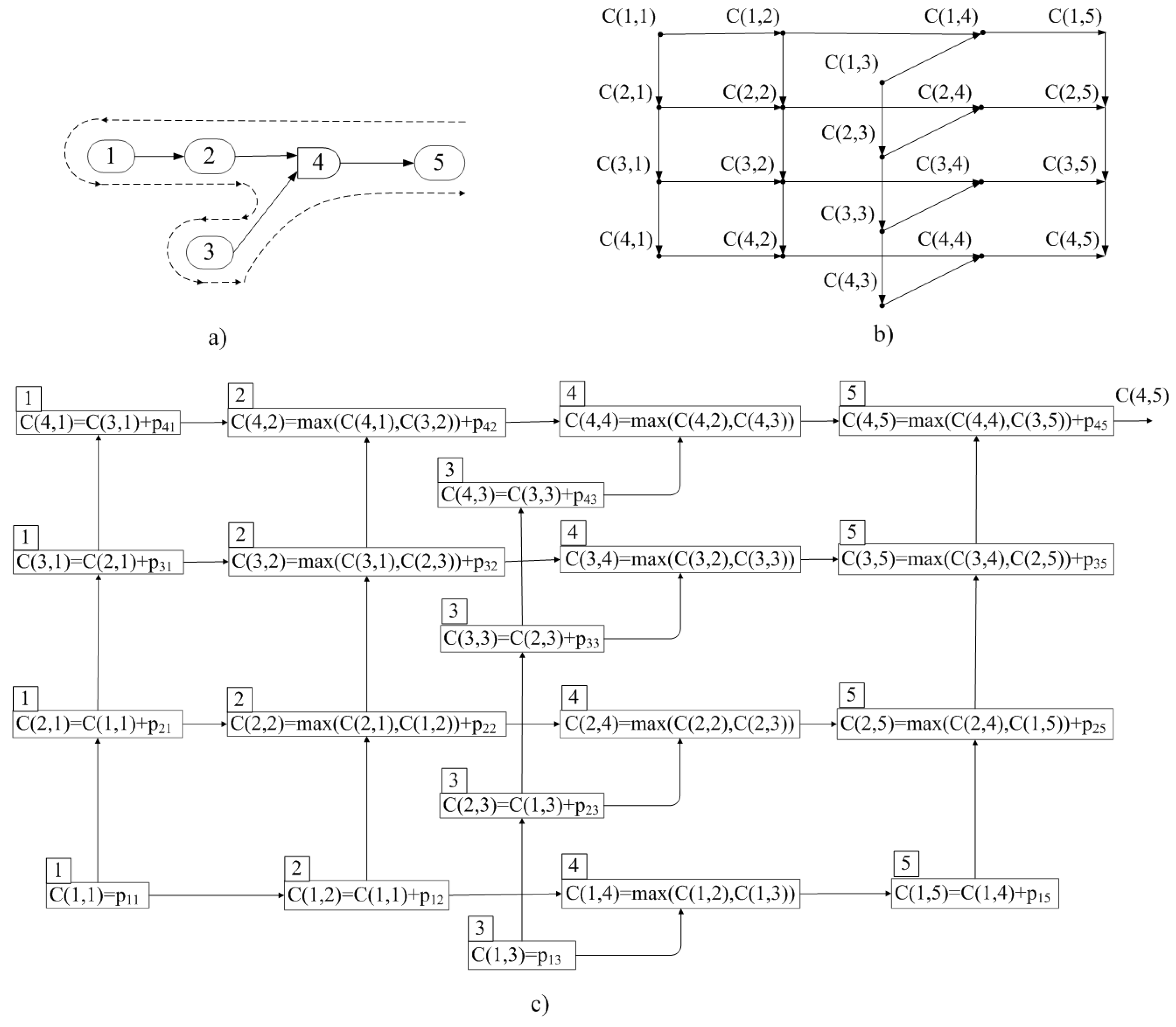
Figure 8a shows the example of a precedence graph between the machines.
Figure 8b shows the precedence graph between machines and jobs (with a fixed order of jobs).
Figure 8c shows the computation (superposition) graph of the recursive function for a certain sequence of 4 jobs. In the latter case, the arc determines the transfer of the value
.
Adding the
function to the PFSP causes the machines to process a job according to the precedence tree.
Figure 8 shows an example of a precedence graph between the machines (
Figure 8a), the corresponding precedence graph between the machines and jobs (
Figure 8b), and the graph of computation (superposition) of the recursive function for some sequence of 4 jobs. The graph in
Figure 8b is acyclic. In this case, it is convenient to traverse the graph according to the jobs, i.e., the 1st job tree, the 2nd job tree, etc. in accordance with the job permutation algorithm. The tree of each job is traversed as indicated in the figure by the dotted line.
6. Implementation of the Branch and Bound Method for the APFSP
When implementing any method for the APFSP, it is necessary to switch to a precedence graph representation with typed vertices. Let us define the set as the following types of vertices:
– the starting vertex of the graph (machine);
– intermediate or final vertex of a graph (machine);
– the vertex corresponding to the function.
Let us define the function that gives the type of a vertex. It is necessary to define explicitly the precedence functions for the vertices .
is defined for the vertices of type , means that the vertex precedes the vertex .
and are defined for the vertices of type , means that the vertex precedes the vertex along the first incoming edge, means that the vertex precedes the vertex along the second incoming edge.
The main issues of the implementation of the method are also the choice of the lower bounds (LB) calculating techniques and branching algorithms. Consider the calculation of the lower bound LB1 by traversing the jobs, that is, similar to
Figure 5, but with tree traversal. This means that formulas (
10) and (
19) are used.
Evaluation of the Lower Bound LB1. The analysis of the formula (
10) shows that when calculating the function
, the operations
are traversed in the order indicated in
Figure 5a. Consider the example in
Figure 8a. If the
function is present, the job processing tree will be traversed as shown in the figure. Naturally, the value of
is calculated after calculating
. The values of
for the job
considering that
can be calculated as follows:
From the example considered, it is clear that the calculation of
is carried out using the same tree traversal as when calculating
. In this case, for
, Equality (
16) is transformed into the equality
where
is the set of vertices belonging to the path from
to
m in the machine precedence graph. The uniqueness of this path follows from the fact that the machine precedence graph is a tree, and
m is its root node (see, for example,
Figure 8a or b). Taking into account Remark 1, the expression (
17) can also be used.
The Appendix presents three algorithms used for the solution of the problem AFS.
The described algorithms work both for the PFSP and the APFSP. The only difference is in the definitions of the function. In the case of the PFSP, . For the APFSP, the precedence functions are determined from the precedence graph or a matrix. In this case, it is obvious that for the APFSP, the complexity of the B&B algorithm does not increase. An important feature should be noted. In the case when the last vertex in the precedence graph is the function, the B&B algorithm executes correctly, but its ”predictive power” is reduced to zero.
Recursive functions allow one to calculate also the values of objective functions different from makespan. This can be done by replacing the function
by
In this case, the calculation of the optimization criterion is concentrated in the body of the function
and is invariant to the details of the optimization method.
7. Evaluating the Effectivenes of the Algorithm
The existing publications on the B&B method in the scheduling theory use tests that are characterized by the processing times on specific machines. To assess the effectiveness of the B&B method, without using pure processing time indicators, it is advisable to determine how much less of some elementary calculations were completed due to the fact that some sets of job permutations were deliberately discarded and not checked. There are two possible approaches here:
consider it elementary to calculate the completion time of the job’s last technological operation (approach L);
consider it elementary to calculate the completion time of each technological operation of each job (approach A).
In both cases, it is necessary to determine the maximum possible number of such calculations when solving a problem for n jobs and m machines, and then to compare it with the number of calculations actually performed.
In the L approach, the maximum number of elementary computations is determined by the permutation generation algorithm (see Appendix). At each step, this algorithm either adds a new job to the already fixed initial part of the vector , or replaces the last job in this fixed part by the next one. In both cases, the completion time of the last technological operation of the last job in the fixed part of is calculated. The completion times of all technological operations of all previous jobs are already known and do not need to be calculated again. Thus, an ”elementary computation” is the calculation of m elements of the job completion times matrix () row, and the total number of such computations is equal to the number of different variants of the initial part of the vector generated by the algorithm.
Consider, for example, the generation of permutations and the computation of the completion times for three jobs (
3). If the rejection of branches of the search along the lower bound
is never performed, then the sequence of actions performed by the algorithm is described by
Table 3.
As a result of the algorithm’s operation, 15 initial parts of the vector
were generated (including 6 complete permutations of three tasks), and 15 elementary computations of the
rows were performed. With the size
h of the initial part of the vector
, the total number of such generated initial parts is equal to the number of placements from
n to
h:
The total number of initial parts of the vector
of all possible sizes from 1 to
n is equal to
When using the B&B method, the algorithm will perform all
elementary calculations extremely rarely. However, this estimate is achievable in practice. Let us consider the degeneration case in which all rows of the matrix
are identical. In this case, the
value calculated using formulas (
16) or (
17) will be the same for any values of the arguments, and none of the branches will be discarded. The number of elementary calculations performed by the algorithm will be exactly
. In approach
A, the maximum possible number of elementary calculations is
m times
since every row of the job completion times matrix contains
m elements. In the optimized algorithm, the number of real calculations will be less than the given values. The effectiveness of solving a problem can be assessed by the proportion of calculations not performed. If
and
are the numbers of calculations when solving problem number
i for
n jobs and
m machines using the approaches
L and
A, respectively, then the efficiency of the solutions can be estimated using the following formulas:
A zero value of these indicators means that the use of the method did not provide any gain in the number of calculations; a theoretically unattainable value of 1 (or 100%) means that the use of the method completely eliminated the need for calculations.
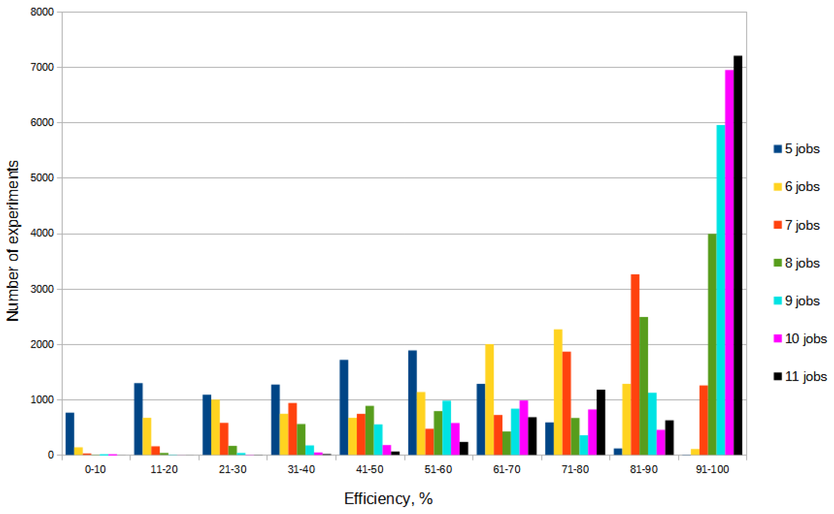
The authors performed 10,000 tests for problems with 5–11 jobs on random acyclic graphs with random job processing times. The problem generation parameters in these experiments were as follows:
total number of nodes in the acyclic graph (technological operations): 15;
number of initial operations: random value in [1,3];
number of ”and” operations: random value in [1,4];
job processing times (): random value in [1,10].
All random values are uniformly distributed integers. For each number of jobs, a histogram of the number of experiments distribution by the ranges of the
efficiency obtained in the experiment was constructed. Thus, 7 histograms were constructed, presented in
Figure 9.
The histograms in the figure show how many times a particular efficiency was achieved during the random experiments. The horizontal axis shows the ten-percent efficiency ranges (from ”0–10” to ”91–100”), and the vertical axis shows the number of experiments out of 10,000 performed in which the corresponding efficiency value was achieved. It can be seen from the figure that as the number of jobs increases, the efficiency of the algorithm also increases. The histogram for five jobs has a maximum around 50%. This means that most of the experiments with five jobs showed a fifty percent efficiency, that is, approximately half of the maximum possible number of elementary calculations for a given task were performed. However, a significant number (about 800) of experiments showed an efficiency of less than 10%. As the number of jobs increases, the histogram maximum moves into the high efficiency region. For eleven jobs, more than 7,000 out of 10,000 experiments performed showed an efficiency in the range of 91–100%, i.e., less than 10% of the number of elementary calculations that would be required to solve the problem when analyzing all possible permutations were performed.