Preprint
Article

This version is not peer-reviewed.

Adaptive GCN and Bi-GRU Based Dual-Branch for Motor lmagery EEG Decoding

A peer-reviewed article of this preprint also exists.

Submitted:

28 November 2024

Posted:

29 November 2024

You are already at the latest version

Abstract

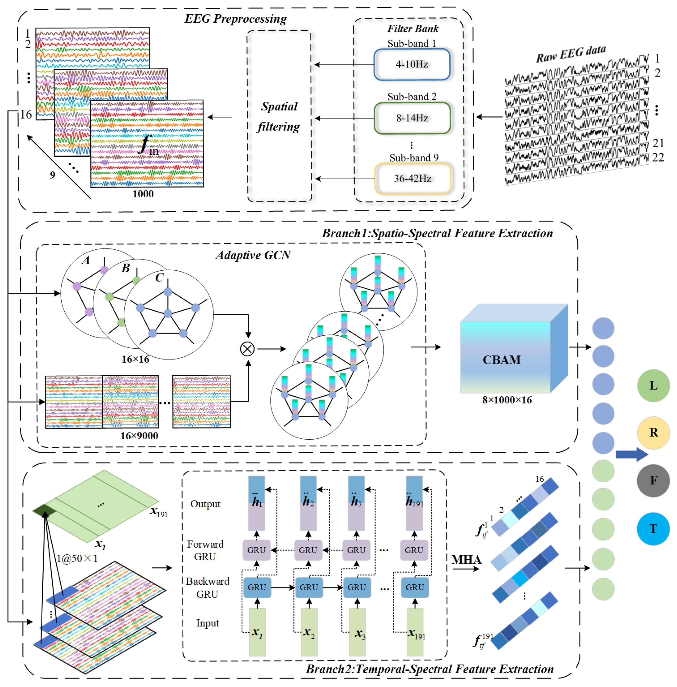
Decoding motor imagery electroencephalography (MI-EEG) signals presents significant challenges due to the difficulty in capturing the complex functional connectivity between channels and the temporal dependencies of EEG signals across different periods. These challenges are exac- erbated by the low spatial resolution and high signal redundancy inherent in EEG signals, which traditional linear models struggle to address. To overcome these issues, we propose a novel dual- branch framework that integrates an Adaptive Graph Convolutional Network (Adaptive GCN) and Bidirectional Gated Recurrent Units (Bi-GRU) to enhance the decoding performance of MI-EEG sig- nals by effectively modeling both channel correlations and temporal dependencies. The Chebyshev Type Il filter decomposes the signal into multiple sub-bands giving the model frequency domain insights. The Adaptive GCN, specifically designed for the MI-EEG context, captures functional connectivity between channels more effectively than conventional GCN models, enabling accurate spatial-spectral feature extraction. Furthermore, combining Bi-GRU and Multi-Head Attention (MHA) captures the temporal dependencies across different time segments to extract deep time-spectral features. Finally, feature fusion is performed to generate the final prediction results. Experimental results demonstrate that our method achieves an average classification accuracy of 80.38% on the BCI-IV Dataset 2a and 87.49% on the BCI-I Dataset 3a, outperforming other state-of-the-art decoding approaches. This approach lays the foundation for future exploration of personalized and adaptive brain-computer interface (BCI) systems.

Keywords: 
;  ;  ;  ;  ;  ;  

1. Introduction

Motor Imagery Brain-Computer Interface (MI-BCI) enables direct interaction between the brain and external devices by decoding electrical activity from the central nervous system [1,2,3]. This technology is valuable in medical rehabilitation [4] and stroke treatment [5]. However, electroencephalogram (EEG) signals are characterized by low signal-to-noise ratios [6], non-stationarity [7], and significant inter-individual variability, posing substantial challenges for decoding EEG signals [8].
Machine learning techniques have been widely applied in the decoding of Motor Imagery Electroencephalogram (Ml-EEG) signals.The Common Spatial Pattern (CSP) is a commonly used method for spatial feature extraction [9], which enhances the separability of signals by maximizing the variance between classes. The Filter, Bank CSP (FBCSP) overcomes the frequency-band dependence issue of CSP [10]. Mojgan et al. [11] adopted root-mean-square and waveform length as temporal features, achieving better performance than CSP. Liu et al. [12] reached an accuracy 93.31% by using Power Spectral Density (PSD) features. Zhang et al. [13] decomposed EEG signals into sub-bands with wavelet packets, extracted temporal-spectral features through an autoregressive model, and classified them using a Support Vector Machine (SVM). Yang et al. [14] utilized Riemann covariance across multiple frequency bands and achieved an accuracy 76%. Despite these advancements, machine learning methods rely on manual feature extraction and are unable to reveal deep latent features, thus limiting the decoding performance of MI-EEG.
With the rapid development of deep learning, many studies in recent years have applied deep learning methods such as convolutional neural networks (CNNs), long short-term memory networks (LSTMs) [15], and recurrent neural networks (RNNs) [16] to EEG signals, achieving good decoding results. Alhagry et al. [17] proposed using the LSTM method to study the time-varying characteristics of EEG. Li et al. [18] proposed a bidirectional ConvLSTM model applied to EEG to explore deep temporal features. Schirrmeister et al. [19] proposed the Shallow ConvNet model, Lawhern VJ et al. [20] proposed the EEGNet model, and models such as Multi-branch-3D [21] and MSFBCNN [22] achieved good classification results in an end-to-end manner without requiring prior knowledge .
The above deep learning methods based on convolutional and recurrent units can easily obtain hidden features through network training. However, when subjects perform MI tasks, the activation intensity of different brain regions varies significantly, and the spatial distribution of EEG signals is irregular [23], making CNNs unable to handle the connectivity between MI-EEG channels [24,25]. In recent years, graph convolutional networks (GCNs) have been proven to capture the relationships between channels using adjacency matrices [26,27,28]. Zhang et al. [29] proposed the GCB-Net generalized graph convolutional network, extracting deeper spatial-spectral information. Song et al. [30] proposed a dynamic graph convolutional neural network that dynamically learns the graph structure of EEG signals through network training. Chen et al. [31] combined the self-attention mechanism and spatial graph convolution to fully utilize the correlations between EEG channels, constructing a classification model that obtained richer spatial features .
The channel connectivity, temporal dependency, and frequency domain information of MI-EEG are all crucial for improving decoding performance. This is because the signals induced by motor imagery in the sensory-motor cortex exhibit event-related desynchronization/synchronization (ERD/ERS) at specific rhythms, brain regions, and time segments. To fully exploit multi-domain features, some researchers have proposed feature fusion methods. Tang et al. [32] proposed the SF-TGCN model, utilizing multi-layer temporal convolution modules and the Laplacian operator to achieve deep temporal and spatial feature fusion of MI-EEG. Li et al. [33] utilized temporal convolution blocks and multi-level wavelet convolution to achieve temporal-frequency feature fusion, achieving an accuracy of 74.71% in four-class motor imagery classification tasks .
However, existing studies only aggregate information from two dimensions, without fully utilizing temporal, frequency, and spatial information simultaneously. Therefore, this paper proposes a dual-branch network to simultaneously explore the channel connectivity, temporal dependency, and frequency domain information of MI-EEG: one branch uses Adaptive GCN to establish the connectivity between channels, capturing the synchronization state and dynamic process of the brain, and employs CBAM to focus on important features, achieving spatial-spectral feature extraction. The other branch employs temporal convolution to serialize the MI-EEG, utilizing Bi-GRU and multi-head self-attention mechanisms to extract deep temporal-spectral features from the dependency relationships in the sequence. Feature fusion is then performed. The main contributions of our work are:
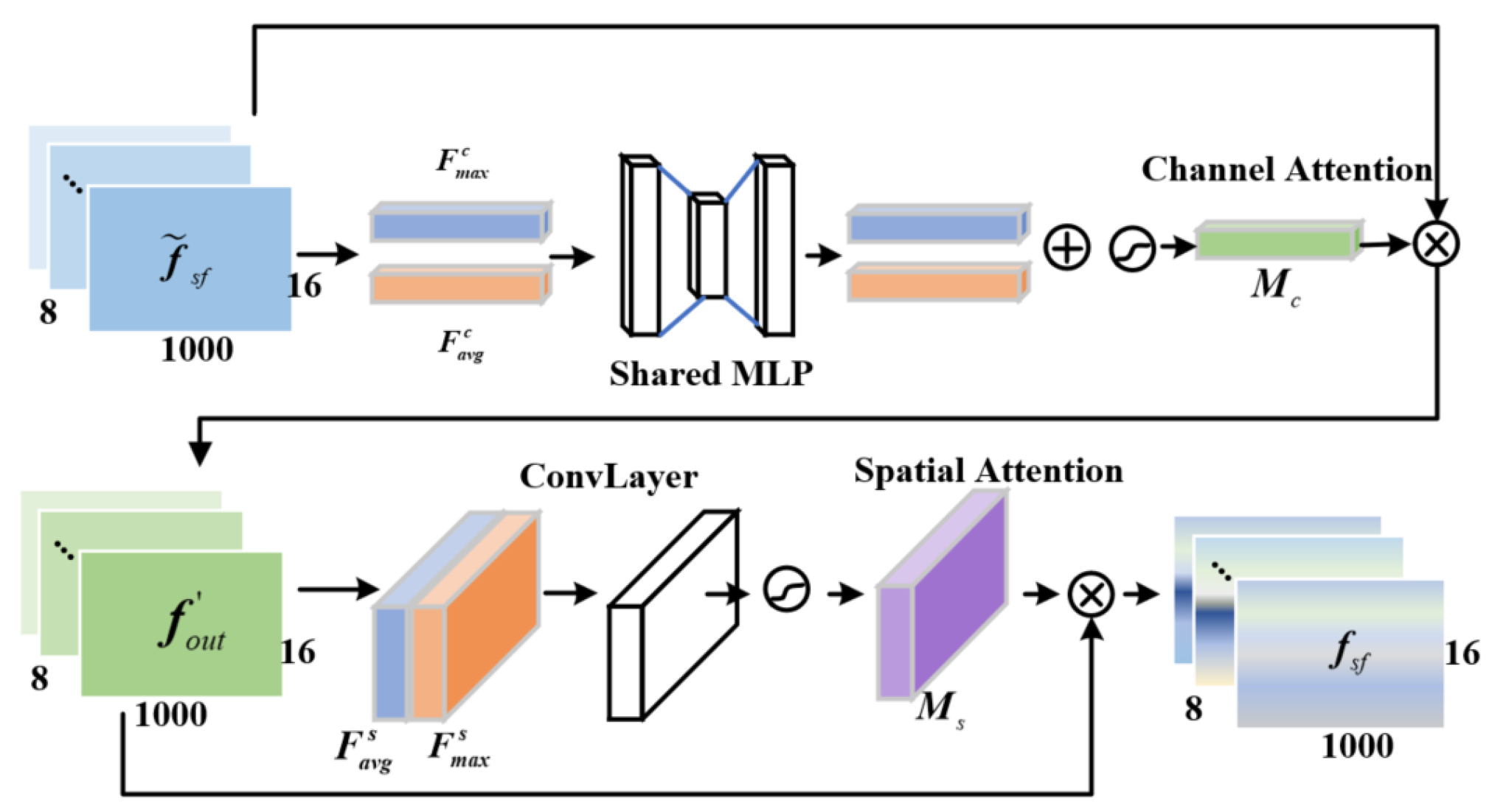
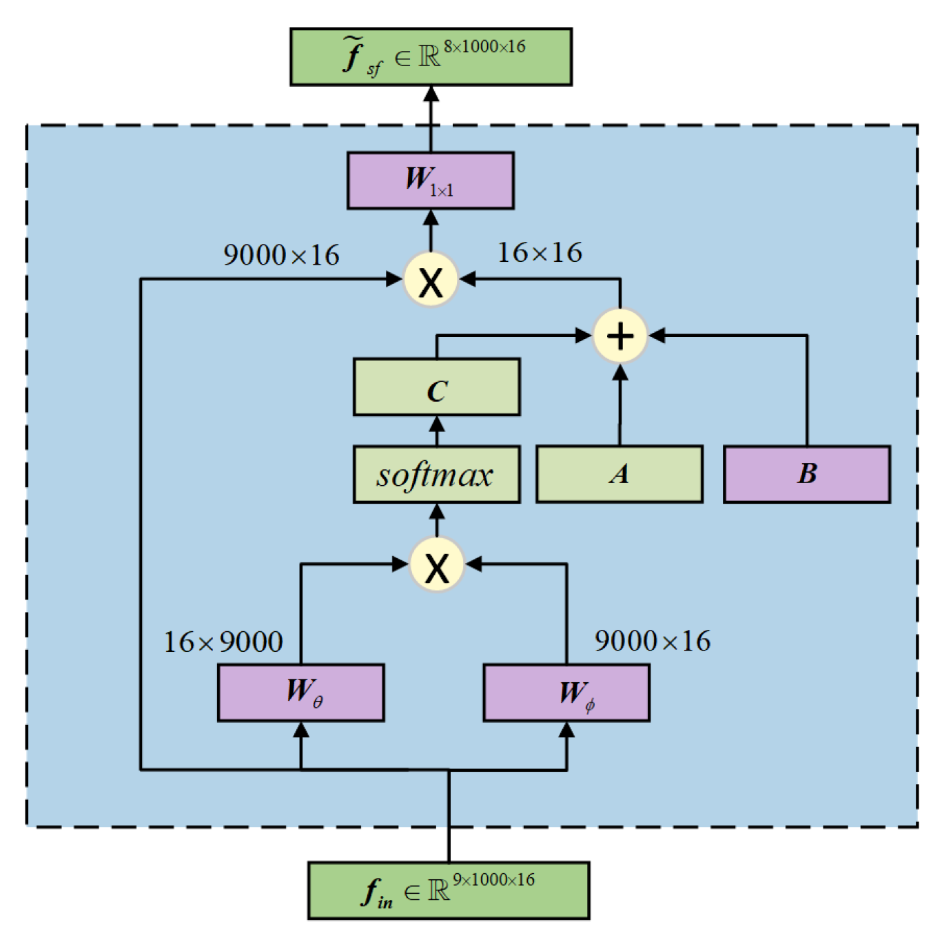
  • An adaptive graph convolutional network is proposed, which constructs the graph convolutional layers of MI-EEG signals using a dynamic adjacency matrix. The CBAM is employed to focus on important features, capturing the synchronized activity states and dynamic processes of the brain, thereby improving the quality of spatial-temporal feature decoding.
  • Propose a time-frequency feature extraction model to fully explore the sequential dependencies and global dependencies among features of different time segments. This study combines the bidirectional gated recurrent unit (Bi-GRU) with the multi-head self-attention mechanism to obtain deep-level time-frequency features.
  • Experiments on multiple public EEG datasets show that, compared with state-of-the-art methods, the proposed model achieves significant improvements, enhancing the decoding quality of MI-EEG multi-classification tasks.
The rest of this paper is organized as follows. Section 2 describes the proposed network structure. Section 3 details the experimental results. Section 4 discusses the effect of the proposed method on the utilization of channel correlation and temporal dependence. Finally, the paper is summarized in Section 5.

2. Materials and Methods
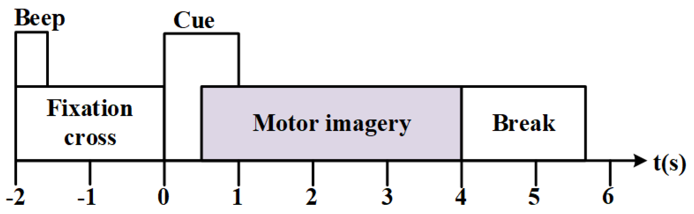
2.1. Dataset

This study utilized the BCI-IV Dataset 2a and BCI-III Dataset 3a, which involve four categories of body movement imagery tasks: left-hand, right-hand, both feet, and tongue.
The BCI-IV Dataset 2a comprises EEG data from nine subjects (A01-A09), with each subject performing 576 motor imagery tasks. Each task lasted approximately 8 seconds, including a 2-second task warning period, a 4-second motor imagery period, and a 2-second rest period. EEG signals were recorded from twenty-two channels at a sampling frequency of 250 Hz. Post-acquisition, bandpass filtering from 0.5 to 100 Hz and 50 Hz notch filtering were applied (Figure 1).
The BCI-III Dataset 3a includes EEG data from three participants (K3b, K6b, L1b), with K3b having 360 trial sets and the other two participants having 240 trial sets each. Each imagery task lasted 4 seconds, with EEG signals recorded from 60 channels at a sampling frequency of 250 Hz. To align with the channel selection in BCI-IV Dataset 2a, 22 electrodes near the central scalp region were selected.

2.2. Proposed Model Framework

This work proposes a dual-branch network using Adaptive GCN and Bi-GRU to enhance MI-EEG decoding performance by simultaneously mining channel correlation and temporal dependency. The model architecture, shown in Figure 2, includes preprocessing, spatio-spectral feature extraction, temporal-spectral feature extraction, and feature fusion. In preprocessing, the original signal is segmented into nine sub-bands, with spatial filtering applied to each to obtain ERD/ERS modes across various frequency bands. Branch I utilizes Adaptive GCN and CBAM to extract spatial-spectral features from EEG channel functional connectivity, leveraging an adaptive adjacency matrix to capture synchronous brain activity states and dynamic processes. Branch II employs Bi-GRU and MHA to extract temporal-spectral features by capturing temporal dependencies in multi-band EEG sequences. Finally, a feature layer fusion strategy is adopted to integrate diverse information, which is then sent to the Softmax layer for classification.

2.3. Preprocessing

Distinguishing motor imagery actions can be achieved through event-related synchronization (ERS) and desynchronization (ERD) [34], which are prominent in the α (8∼13 Hz) and β (14∼30 Hz) bands. To preserve ERD/ERS modes at different frequencies, subband division and CSP-based spatial filtering are applied to the original MI-EEG, inspired by the FBCSP [35] algorithm.
A filter bank was constructed using nine overlapping Chebyshev Type II bandpass filters, each with a 6 Hz bandwidth, covering a range of 4∼42 Hz (4∼10, 8∼14, ..., 36∼42 Hz). Each sub-band is spatially filtered as follows:
Z b , i = W ¯ b T E b , i
where Z b , i is the signal after spatial filtering, E b , i R c × t represents the i-th EEG sample in the b-th frequency band, c is the number of EEG channels, t denotes the number of sampling points per channel, and T is the transpose. W ¯ b represents the CSP projection matrix derived from the eigenvalue decomposition of Eq. 2:
Σ b , 1 W b = ( Σ b , 1 + Σ b , 2 ) W b D b
where Σ b , 1 and Σ b , 2 represent the covariance matrix estimates for the first and second classes of MI tasks in the b-th frequency band, respectively, D b is a diagonal array consisting of the eigenvalues of Σ b , 1 . The first n and the last n column vectors from W b R c × c are selected to form the spatial domain filter W ¯ b . For the four-class MI tasks, a One-vs-Rest strategy is adopted. One MI task is considered the first class, while the other tasks are combined into the second class. The final spatial filter W ¯ b contains k × 2 × n vectors, where k = 4 represents the four classifications, and n = 2 is set. After spatial filtering according to Eq. 1, the number of EEG channels is 16. After spatial filtering of the 9 band signals, the dimension of the input data f i n becomes 9 × 1000 × 16 .

2.4. Spatio-Spectral Feature Extraction Module

EEG exhibits complex dynamic functional connections between different brain regions. Graph convolutional networks have been proven to capture the correlation between channels effectively. Therefore, a spatio-spectral feature extraction module is designed to capture EEG channel correlations across frequency bands and fully extract spatio-spectral features.
The topology of MI-EEG must first be constructed to process EEG signals using graph convolution [36]. An undirected EEG signal connectivity graph is denoted as G = { V , E , A } , where V = { v 1 , v 2 , , v i , v N } represents the set of nodes, v i denotes the electrode channel, E is the set of edges connecting the nodes, and ( v i , v j ) E , A = { a i j R N × N ; i , j = 1 , , N } represents the adjacency matrix describing the connection strength between any two nodes. In constructing A, the traditional approach considers the electrode distribution as a non-Euclidean space, representing the spatial disorder of the local EEG channel by the adjacency of electrode nodes. Since the ERD/ERS phenomenon in MI-EEG is distributed across multiple brain regions, electrode interactions must be reflected globally. In this paper, A is constructed using the Pearson correlation coefficient P, as in Eq. 3, which captures synchronous brain activity information and retains the negative correlation of EEG channel activity by taking the absolute value of P. Additionally, introducing the self-connectivity coefficient α enhances the weight of the self-node.
A = P + α I
Since motor imagery is a dynamic process, Adaptive GCN [37] was used in constructing MI-EEG graphs to capture dynamically changing brain connectivity states. This method allows for adaptive adjustment of graph connection weights and enhances the extraction of deep spatio-spectral features.
Specifically, the spatio-spectral features f ˜ s f obtained by Adaptive GCN are computed as follows:
f ˜ s f = W 1 × 1 * ( D ˜ 1 / 2 A D ˜ 1 / 2 + B + C ) f i n
The adjacency matrix A R N × N is calculated using Eq. 3, D ˜ is the degree matrix used to standardize A . B R N × N represents the shared adjacency matrix for all samples, retaining common information. It is a trainable parameter that is dynamically updated during model training. The update process follows Eq. 5, with r as the learning rate and L o s s as the model training loss.
B = ( 1 r ) B + r L o s s B
C R b s × N × N represents the adjacency matrix associated with the sample data, assigning unique connection strengths to each input data, computed as in Eq. 6, W θ and W ϕ denote two 1*1 convolution kernels.
C = s o f t m a x ( f i n T W θ T W ϕ f i n )
Redundant information exists in the spatio-spectral features f ˜ s f extracted by Adaptive GCN. Therefore, this paper introduces CBAM [38] (Figure 3), which uses an attention mechanism in both feature space and feature channel dimensions to suppress redundant features and improve the quality of the spatio-spectral features.
Feature channel attention emphasizes important feature channels. The spatial dimensionality of f ˜ s f is compressed using average and maximum pooling to generate the matrices F a v g c and F m a x c , respectively. A multilayer perceptron (MLP) then generates the channel attention mapping M c :
M c ( F ) = σ ( W 1 ( W 0 ( F a v g c ) ) + W 1 ( W 0 ( F m a x c ) ) )
Where σ represents the sigmoid function, W 0 and W 1 are the weights of MLP. Feature space attention emphasizes the target region of interest, complementing channel attention. It is computed as in Eq. 8 by applying average and maximum pooling along the feature channel dimensions to obtain the matrices F a v g s R 1 × 1000 × 16 and F m a x s R 1 × 1000 × 16 . These matrices are concatenated and then convolved with a 3 × 3 kernel to generate M s .
M s ( F ) = σ ( f 3 × 3 ( [ A v g P o o l ( f o u t ) ; M a x P o o l ( f o u t ) ] ) ) = σ ( f 3 × 3 ( [ F a ν g s ; F m a x s ] ) )
The feature f ˜ s f is element-wise multiplied with M c R 8 × 1 × 1 and M s R 1 × 1000 × 16 to obtain the weighted spatio-spectral feature f s f .
f o u t = M c ( f ˜ s f ) f ˜ s f f s f = M s ( f o u t ) f o u t
Figure 4 presents the implementation details of the AGCN layer, which combines the AGCN layer, batch normalization (BN), and the ReLU activation function to form a foundational graph convolutional network (GCN) module. Multiple GCN modules are then stacked to construct the complete graph convolutional network.

2.5. Temproal-Spectral Feature Fxtraction Module

MI-EEG is a highly time-varying signal, dependent on preceding and succeeding time segments [39]. To fully leverage the temporal dependencies and enhance MI-EEG decoding performance, this paper proposes a temporal-frequency feature extraction module, comprising a temporal convolution layer, a single-layer Bi-GRU, and an MHA module. The temporal convolution layer consists of a two-dimensional convolution filter of size (50, 1). The input is f i n R 9 × 1000 × 16 , and the output is the temporal-spectral feature x R 16 × 191 = [ x 1 , . . . , x t , . . . , x 191 ] . Each sequence x t in x aggregates the temporal-spectral information of a 0.2s time window (the sampling frequency is 250Hz, and 50 sampling points are recorded in 0.2s). The Bi-GRU [40] model captures the forward and backward dependencies of the sequence x t . Bi-GRU, a type of RNN with a gating structure, includes an update gate z t and a reset gate r t . This gating structure selectively transfers information in the hidden layer, solving the gradient vanishing problem in RNNs and overcoming short-term memory issues, as calculated by the following formulas:
r t = σ ( W r x t + U r h t 1 + b r )
z t = σ ( W z x t + U z h t 1 + b z )
W , U , b are the weight parameter matrices and bias, respectively. h t 1 represents the hidden state of the ( t 1 ) t h temporal-spectral sequence containing all information before the ( t 1 ) time slice. σ is the sigmoid nonlinear activation function. Using the update gate z t and reset gate r t , the hidden layer state information h t of the current sequence x t is computed as shown in Eq. 12, h ˜ t represents the candidate hidden state, and ⊙ denotes element-wise multiplication.
h ˜ t = tanh ( W h x t + U h ( r t h t 1 ) + b h ) h t = ( 1 z t ) h t 1 + z t h ˜ t
Bi-GRU computes the hidden states h t and h t from the forward and backward directions, and concatenates them to obtain the temporal-spectral feature h t , which contains both forward and backward dependencies. To improve the model’s capacity to capture long-range dependencies within the sequences, the MHA [41] is employed to capture global dependencies among h t . The MHA module performs self-attention computations with multiple attention heads and outputs the final temporal-spectral feature f t f following a linear transformation, W O represents the weight matrix.
f t f = [ head 1 ; . . . ; head i ; . . . ; head h ] W O
head i = s o f t m a x ( QW Q i · ( KW K i ) T d k ) VW V i
Each attention head is computed as in Eq. 14, Q , K , V are the matrices obtained by linear transformation of h t , W Q i , W K i , W V i represent the trainable weight matrices, and d k = 16 is the feature dimension of the sequence h t .

2.6. Feature Fusion

The extracted spatio-spectral features f s f and temporal-spectral features f t f are fused. The features f s f and f t f are reduced to 8 and 16 dimensions using average aggregation. The spliced features are linearly transformed using a single-layer neural network, as shown in Eq. 15, with W and b as the weights and bias. The features are converted into probabilities using the Softmax function in Eq. 16 for normalization and dividing EEG into four categories.
x = W 4 × 24 ( [ Avgagg ( f s f ) , Avgagg ( f t f ) ] ) + b 4 × 1
x o u t ( i ) = exp ( x ( i ) ) k = 1 4 exp ( x ( k ) ) , i = 1 , . . . , 4

3. Results

3.1. Software and Hardware Environment

The models were implemented in a Python 3.9 environment using the PyTorch 1.13.1 framework and executed on a GeForce 3050 GPU. Model parameter settings are detailed in Table 1. The final results were derived from the average of five separate experiments, using an 8:2 split ratio for training and test sets.

3.2. Classification Results

The classification performance of our proposed dual-branch network across subjects is summarized in Table 2. On average, the model achieved an accuracy of 82.16% and a Kappa value of 0.761. Notably, accuracy exceeded 90% for three participants. However, subjects A02 and A06 showed significantly lower accuracies, below 70%, indicating poor classification. To investigate these disparities, we examined the signal characteristics of the subjects, focusing on Event-Related Desynchronization/Synchronization (ERD/ERS) phenomena [42,43].
Utilizing Pfurtscheller’s method [44], this study plotted the ERD/ERS characteristic curves for subjects A03, K3b, A02, and A06. The analysis employed Eq. 17, where A is the signal energy during motor imagery and R is the baseline signal energy, measured during a reference period set from -3 to -2.5 seconds. This detailed approach underscores the significance of signal characteristics in enhancing classification accuracy and highlights potential avenues for improving model performance in subjects with initially low classification accuracies.
E R D / E R S = A R R × 100 % .
Figure 5a and Figure 5b illustrate the ERD/ERS characteristic curves for subjects A03 and K3b, respectively. During motor imagery, movements of the left hand, right hand, both feet, and tongue generally exhibit distinct ERD/ERS characteristics, resulting in better classification outcomes. Figure 5c presents the ERD/ERS characteristic curves for subject A02, where consistent trends and similar energy changes are observed in the C3, C4, and Cz channels during different imagined movements. Figure 5d displays the ERD/ERS characteristic curves for subject A06, where significant ERD is observed in the Cz channel across all fthe proposed method imagined tasks, with consistent trend patterns. These results indicate that subjects A02 and A06 did not elicit corresponding responses in the brain regions associated with different limb movements, lacking separability and resulting in poor classification outcomes.
Table 3 presents the decoding outcomes results of our proposed method and seven baseline methods on the two datasets. The proposed method achieved 80.38% accuracy and 0.737 Kappa on BCI-IV Dataset 2a, and 87.49% accuracy and 0.833 Kappa on BCI-III Dataset 3a, outperforming CSP [9], FBCSP [10], Deep ConvNet [19], Shallow ConvNet [19], and EEGNet. Furthermore, the proposed method achieved the highest results on both datasets compared to the recently proposed EEG-Conformer [45] and LightConvNet [39] models. This superior performance is attributed to the proposed method’s consideration of synchronized activities and dynamic signal changes during the MI-tasks, fully exploiting channel correlation and temporal dependence of the MI-EEG, resulting in better decoding outcomes.
This superior performance is attributed to the proposed method‘s consideration of synchronized activities and dynamic signal changes during the motor imagery, fully exploiting channel correlation and temporal dependence of the MI-EEG, resulting in better decoding outcomes.

3.3. Ablation Experiments

The proposed dual-branch network extracts spatio-spectral and temporal-spectral features of MI-EEG using Adaptive GCN and Bi-GRU, respectively, and performs feature fusion. We conduct comparative experiments to validate the effectiveness of multi-domain feature fusion.
Branch1:Only Adaptive GCN and CBAM are used to extract spatio-spectral features.
Branch2:Temporal-spectral features are extracted using Bi-GRU and MHA.
Our method:Combines temporal-spectral and spatial-spectral features using a dual-branch network.
The experimental results after the feature fusion of the two datasets are shown in Table 4. We present the precision and recall for each type of task to evaluate the model’s performance in recognizing various tasks. For the BCI-IV Dataset 2a, the precision and recall of each task are consistent across the three experiments. However, the classification performance of Branch1 and Branch2 is significantly lower than that of the feature fusion (Our method). For the BCI-III Dataset 3a, when only using Branch1 and Branch2 for classification, each task’s precision and recall distribution are uneven. For example, in Branch1, the left-hand task achieves a high precision but a low recall, indicating that the left-hand task is misclassified as other categories when only spatial-spectral features are extracted. In contrast, the classification results of each task after feature fusion (Our method) are more balanced and significantly higher than those of Branch1 and Branch2. This indicates that the model’s generalization performance is better after feature fusion, proving the importance of feature fusion and the complementarity of different dimensional information.
From Table 4, it can also be seen that the spatial-spectral features of the two datasets are more distinguishable than the temporal-spectral features. This is because the neural activity caused by limb movements has a distinct somatotopic organization. For example, hand movements mainly manifest in the contralateral brain hand functional area, and foot movements activate the central brain area. Compared to time-dimensional information, the spatial distribution differences of signals generated by different limb movements are more significant.

3.4. Comparison Experiments of Adjacency Matrices

The adaptive adjacency matrix in this study comprises three matrices: A, B, and C, capturing synchronous brain activity and dynamic connections. Three experiments were conducted to verify their validity:
Experiment1:Constructing the adjacency matrix using the spatial positioning information of EEG channels [46].
Experiment 2: Constructing the adjacency matrix using only matrix A.
Experiment 3:Constructing the adaptive adjacency matrix using Eq. 4 (our method).The experimental results of classification using different adjacency matrices for the two datasets are shown in Table 4. Comparing Experiment 1 and Experiment 2, adopting matrix A yielded better results than constructing the adjacency matrix based on spatial location information. This is because adjacency relationships can only aggregate information between channels in local brain regions, while synchronous brain activities occur in the whole brain region. Adjacency matrix A can establish connections across all EEG channels, making better use of channel information.
In Experiment 3, for the BCI-IV Dataset 2a, using the adaptive adjacency matrix(Our method) improves the precision of each task by 6.99%, 5.49%, 7.12%, and 5.76%, and the recall by 7.58%, 6.13%, 7.82%, and 5.59% compared to Experiment 2. For the BCI-III Dataset 3a, using the adaptive adjacency matrix(Our method) improves the precision of each task by 11.71%, 5.47%, 6.81%, and 1.33%, and the recall by 4.63%, 5.55%, 11.29%, and 13.52% compared to Experiment 2. The improvement is attributed to our method’s ability to establish whole-brain connectivity and adaptively capture the brain’s dynamic processes, thereby fully exploring brain functional activities.

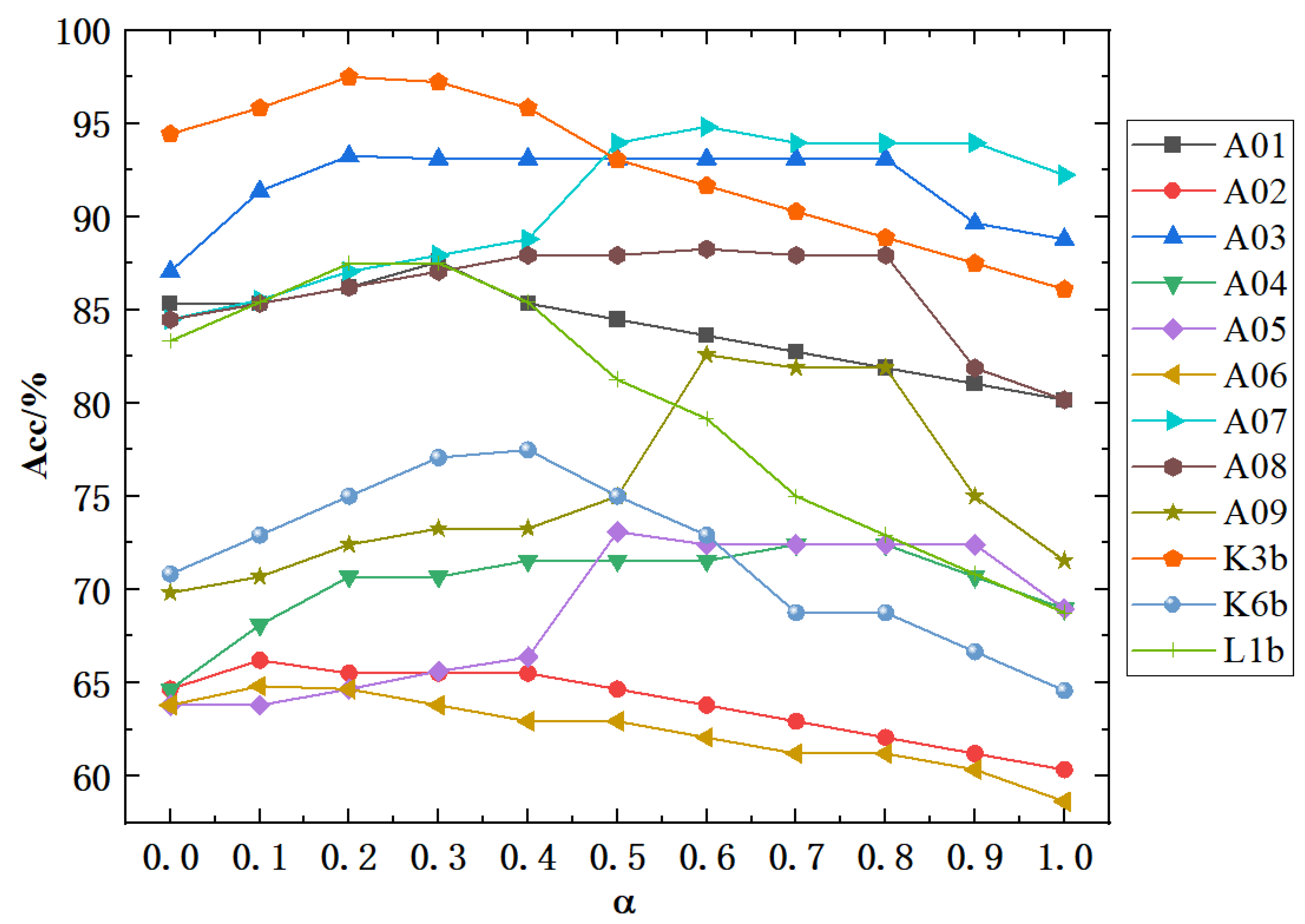
3.5. Effect of Self-Connection Coefficients

Introducing the self-connection coefficient α aims to enhance the utilization of self-channel information, with its value ranging from 0 to 1. To verify the impact of the self-connection coefficient on classification results, we tested values at intervals of 0.1. As shown in Figure 6, classification accuracy increases with the self-connection coefficient for most subjects, reaching a peak before decreasing. This indicates that placing too much or too little emphasis on the node’s information can negatively affect classification performance. The optimal self-connection coefficient varies among subjects, with values of 0.3, 0.1, 0.2, 0.7, 0.5, 0.1, 0.6, 0.6, 0.6, 0.2, 0.4, and 0.2, reflecting the individual differences among the subjects.

4. Discussion

We propose a dual-branch Ml-EEG decoding method using adaptive GCN and Bi-GRU, which can capture the channel correlations and temporal.dependencies among multiple frequency bands.To better understand the advanced nature of the proposed method in capturing brain functional activities and temporal dependencies, we conduct a visual analysis of the adjacency matrix and the output characteristics of each stage of the model.

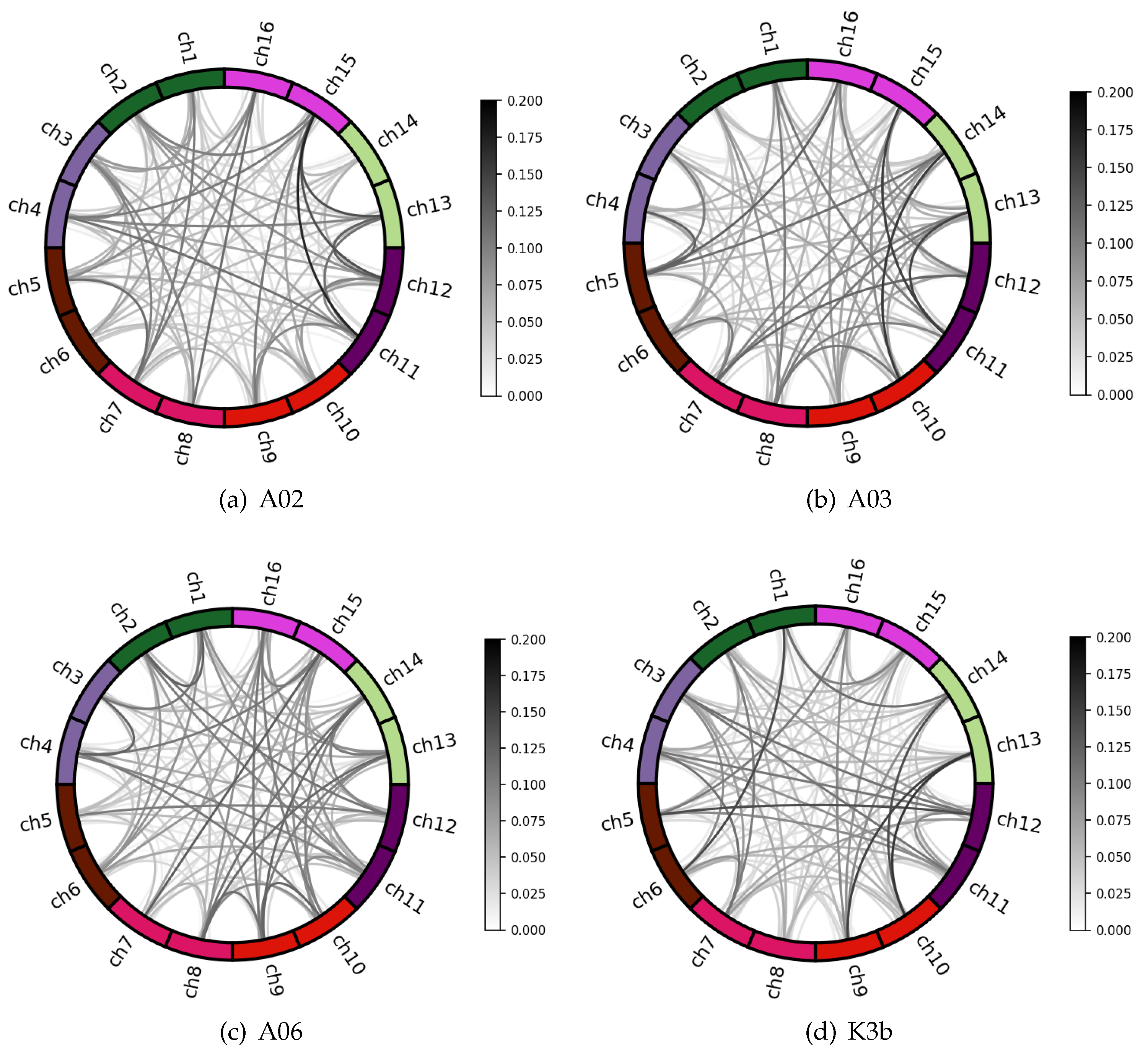
4.1. Channel Correlation Visual Analysis

The weight edges of the adjacency matrix A were visualized to evaluate the impact of graph convolution on MI-EEG channel correlation. Figure 7 shows the brain functional connectivity patterns of different subjects. The outer circle represents different EEG channels, and the inner lines indicate their connectivity properties. Darker lines show a greater correlation, based on Pearson correlation coefficients in adjacency matrix A. Weights are assigned to channel pairs based on correlation, selectively aggregating synchronous activity information. Connection strength varies among subjects, indicating individual differences.

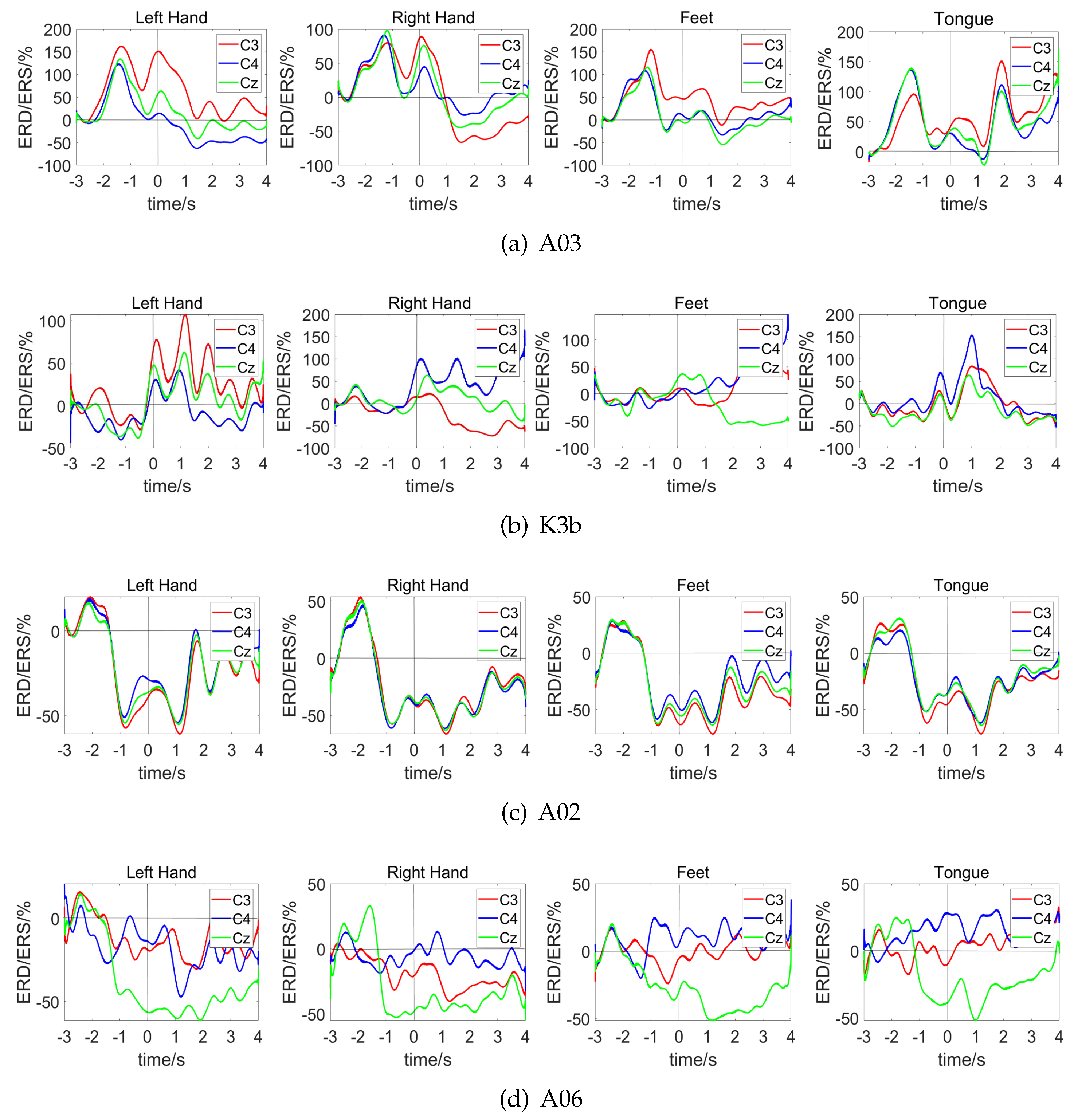
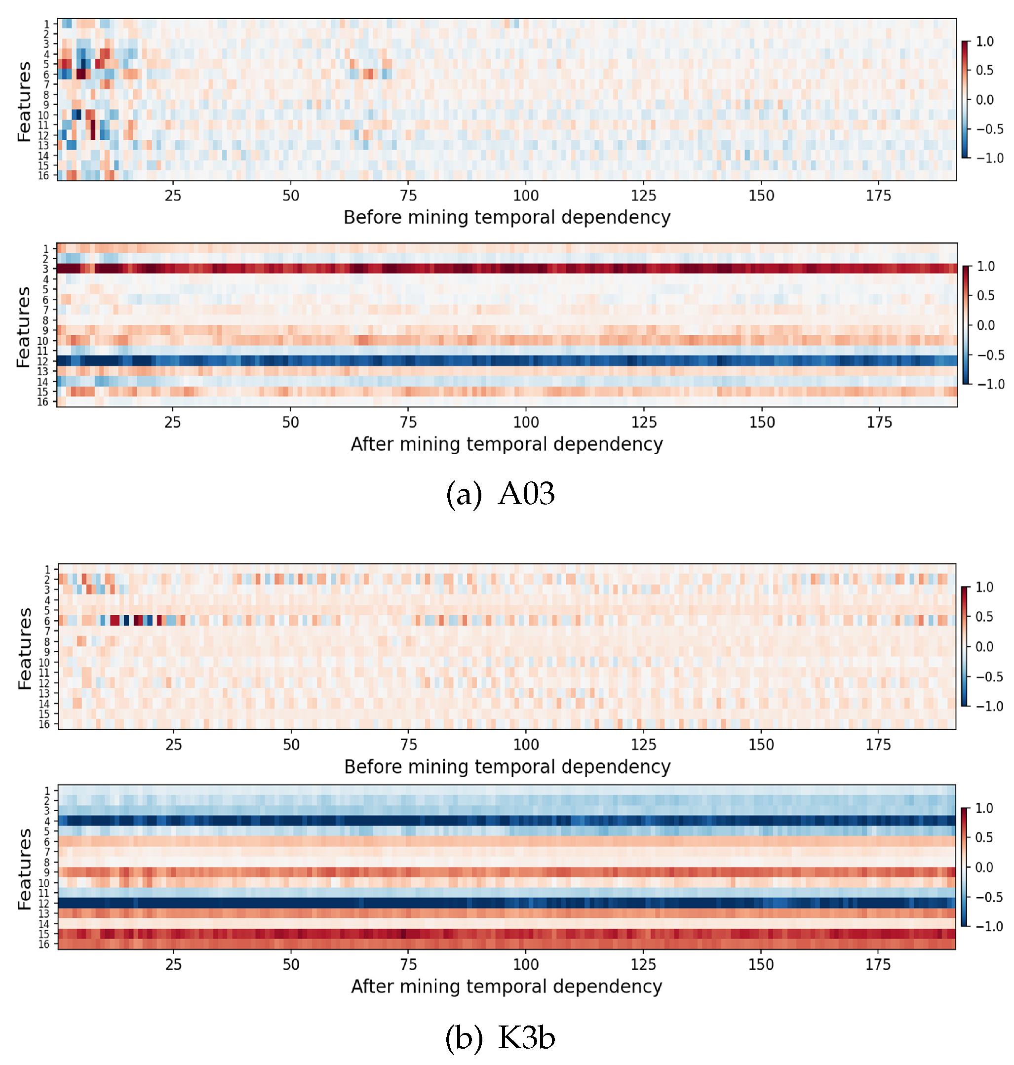
4.2. Time Dependence Visual Analysis

To observe the impact of temporal dependencies on features, the features x before capturing temporal dependencies and features f t f after capturing them for all samples of each subject are obtained, and the feature mean is calculated along the sample dimensions for visualization. The visualization for subjects A03 and K3b is shown in Figure 8. The horizontal axis displays sequences from various time windows, each aggregating data from 50 sample points (0.2 second time window), and the vertical axis represents the sequence features.
Before temporal dependency capture, the feature map is discrete, indicating weak connections between time window sequences. After mining, dependencies strengthen significantly. For example, feature channels 3 and 12 of subject A03 are extremely similar in color throughout the entire time axis, suggesting that these time segments aggregate each other’s information. This shows that Bi-GRU and MHA effectively extract MI-EEG temporal-dependence.
In the feature map before temporal-dependency capture, the first 25 sequences show obvious differences and prominent colors, while other sequences have small feature values. This is because the first 25 sequences correspond to the initial 125 MI-EEG sampling points (0∼0.5s period of the acquisition paradigm), which is the task cueing stage when subjects are in a preparation state. The data from this period generally lack useful information. After temporal-dependent mining, these features are no longer prominent, indicating that Bi-GRU and MHA effectively reduce irrelevance information.

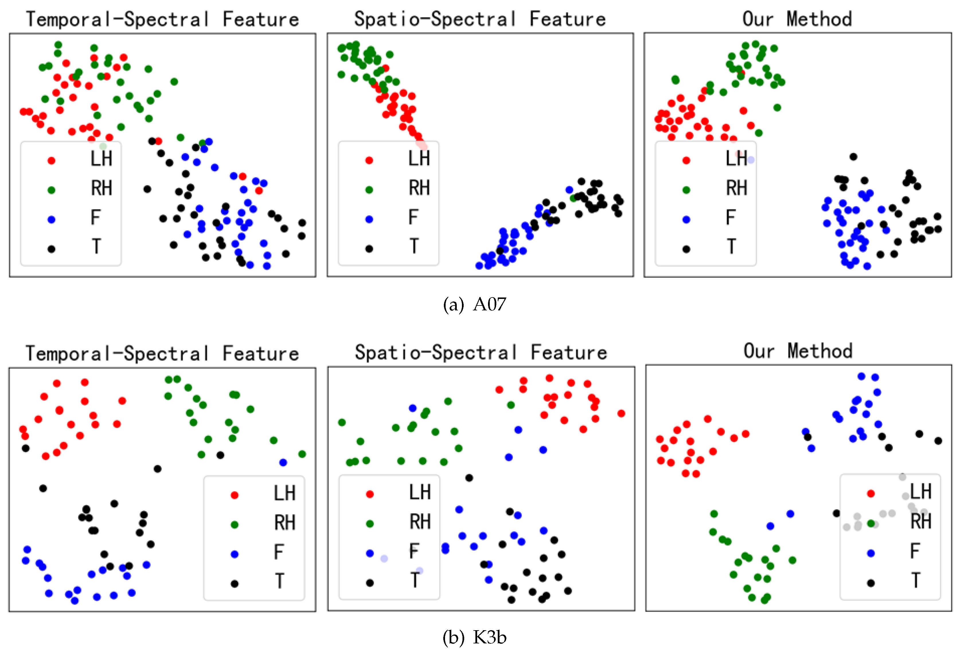
4.3. Feature Fusion Visual Analysis

To visually demonstrate the classification effect of feature fusion, the t-SNE [47] method was used to embed the temporal-spectral features, spatial-spectral features, and fusion features (our method) into two-dimensional scatter plots to observe the degree of feature separation. Figure 9a shows the visualization results of subject A07. For temporal-spectral features, different tasks overlap significantly. For spatial-spectral features, the separability between left and right-hand tasks and between feet and tongue tasks is poor. The inter-class distances between tasks are increased after feature fusion significantly. Figure 9b shows the visualization results of subject K3b. From the temporal-spectral and spatial-spectral features, it can be seen that the left and right-hand tasks introduce individual other samples. However, after feature fusion, the left and right-hand tasks are completely separated from other tasks. This result indicates that integrating the time, frequency, and spatial domain information of MI-EEG can enhance the separability of different tasks.

5. Conclusions

Aiming at the problems that the channel correlations and temporal dependencies among multiple frequency bands of MI-EEG are difficult to capture precisely and efficiently, and the signal decoding quality needs to be improved, we propose a multi-domain feature classification method for MI-EEG based on a dual-branch network. This method uses Adaptive GCN and Bi-GRU to mine the brain functional connectivity and temporal dependencies of MI-EEG respectively. Meanwhile, the CBAM attention mechanism and multi-head self-attention mechanism are introduced to capture the valuable information in features of each dimension, achieving an effective fusion of time-frequency-spatial domain features of MI-EEG and improving the decoding quality. The proposed method is evaluated with two datasets, BCI - IV Dataset 2a and BCI - III Dataset 3a. The results show that our method has higher performance and provides a new approach for MI-EEG decoding.

Funding

This work was supported by the 2023 Industrial Internet Innovation and Development Project-Cross-industry Collaborative Application and Data element Service Platform Project based on Industrial Internet identification analysis System (Project number: CEIEC-2023-ZM02-0090)

Data Availability Statement

Publicly available datasets were analyzed in this study. The BCI Competition IV Dataset IIa can be foundhere: https://www.bbci.de/competition/iv/(accessed on 5 November 2023).The BCI Competition III Dataset IIIa can be foundhere:https://www.bbci.de/competition/iii/.

Conflicts of Interest

The authors declare no conflicts of interest.

References

  1. J. R. Wolpaw and D. J. McFarland, “Control of a two-dimensional movement signal by a noninvasive brain-computer interface in humans,” Proceedings of the national academy of sciences, vol. 101, no. 51, pp. 17 849–17 854, Dec. 2004.https://www.pnas.org/doi/full/10.1073/pnas.0403504101.
  2. K. Tanaka, K. Matsunaga, and H. O. Wang, “Electroencephalogram-based control of an electric wheelchair,” IEEE transactions on robotics, vol. 21, no. 4, pp. 762–766, Aug. 2005.https://ieeexplore.ieee.org/document/1492493.
  3. Y. Wang, B. Hong, X. Gao, and S. Gao, “Implementation of a brain-computer interface based on three states of motor imagery,” in 2007 29th Annual International Conference of the IEEE Engineering in Medicine and Biology Society. IEEE, 2007, pp. 5059–5062.https://ieeexplore.ieee.org/document/4353477.
  4. K. LaFleur, K. Cassady, A. Doud, K. Shades, E. Rogin, and B. He, “Quadcopter control in three-dimensional space using a noninvasive motor imagery-based brain–computer interface,” Journal of neural engineering, vol. 10, no. 4, p. 046003, Aug. 2013.https://iopscience.iop.org/article/10.1088/1741-2560/10/4/046003.
  5. C. Herff, D. Heger, A. De Pesters, D. Telaar, P. Brunner, G. Schalk, and T. Schultz, “Brain-to-text: decoding spoken phrases from phone representations in the brain,” Frontiers in neuroscience, vol. 8, p. 141498, Jun. 2015.https://www.frontiersin.org/journals/neuroscience/articles/10.3389/fnins.2015.00217/full.
  6. C. Tang, T. Zhou, Y. Zhang, R. Yuan, X. Zhao, R. Yin, P. Song, B. Liu, R. Song, W. Chen et al., “Bilateral upper limb robot-assisted rehabilitation improves upper limb motor function in stroke patients: a study based on quantitative eeg,” European Journal of Medical Research, vol. 28, no. 1, p. 603, Dec. 2023.https://eurjmedres.biomedcentral.com/articles/10.1186/s40001-023-01565-x.
  7. M. Xu, X. Xiao, Y. Wang, H. Qi, T.P. Jung, D. Ming, “A brain-computer interface based on miniature-event-related potentials induced by very small lateral visual stimuli,” IEEE Trans. Biomed. Eng., vol. 65, no. 5, pp. 1165-1175, May 2018.
  8. J. Mei, R. Luo, L. Xu, W. Zhao, S. Wen, K. Wang, X. Xiao, J. Meng, Y. Huang, J. Tang et al., “Metabci: An open-source platform for brain–computer interfaces,” Computers in Biology and Medicine, vol. 168, p. 107806, Jan. 2024.https://www.sciencedirect.com/science/article/pii/S0010482523012714?
  9. Z. J. Koles, M. S. Lazar, and S. Z. Zhou, “Spatial patterns underlying population differences in the background eeg,” Brain topography, vol. 2, no. 4, pp. 275–284, 1990.https://link.springer.com/article/10.1007/BF01129656.
  10. K. K. Ang, Z. Y. Chin, H. Zhang, and C. Guan, “Filter bank common spatial pattern (fbcsp) in brain-computer interface,” in 2008 IEEE international joint conference on neural networks (IEEE world congress on computational intelligence). IEEE, 2008, pp. 2390–2397.https://ieeexplore.ieee.org/document/4634130.
  11. M. Tavakolan, Z. Frehlick, X. Yong, and C. Menon, “Classifying three imaginary states of the same upper extremity using time-domain features,” PloS one, vol. 12, no. 3, p. e0174161, Mar. 2017.https://journals.plos.org/plosone/article?id=10.1371/journal.pone.0174161.
  12. S. Liu, J. Tong, J. Meng, J. Yang, X. Zhao, F. He, H. Qi, and D. Ming, “Study on an effective cross-stimulus emotion recognition model using eegs based on feature selection and support vector machine,” International Journal of Machine Learning and Cybernetics, vol. 9, pp. 721–726, May. 2018.https://link.springer.com/article/10.1007/s13042-016-0601-4.
  13. Y. Zhang, B. Liu, X. Ji, and D. Huang, “Classification of eeg signals based on autoregressive model and wavelet packet decomposition,” Neural Processing Letters, vol. 45, pp. 365–378, Apr. 2017.https://link.springer.com/article/10.1007/s11063-016-9530-1.
  14. P. Yang, J. Wang, H. Zhao, and R. Li, “MLP with riemannian covariance for motor imagery based eeg analysis,” IEEE Access, vol. 8, pp. 139 974–139 982, 2020.https://ieeexplore.ieee.org/document/9149576.
  15. P. Wang, A. Jiang, X. Liu, J. Shang, and L. Zhang, “LSTM-Based EEG classification in motor imagery tasks,” IEEE Trans. Neural Syst. Reha Eng., vol. 26, no. 11, pp. 2086–2059, Oct. 2018.https://ieeexplore.ieee.org/document/8496885.
  16. T. Luo, C. Zhou, F. Chao, “Exploring spatial-frequency-sequential relationships for motor imagery classification with recurrent neural network,” BMC BIOINFORMATICS., vol. 19, p. 344, Sep. 2018.https://bmcbioinformatics.biomedcentral.com/articles/10.1186/s12859-018-2365-1.
  17. S. Alhagry, A. A. Fahmy, and R. A. El-Khoribi, “Emotion recognition based on eeg using lstm recurrent neural network,” International Journal of Advanced Computer Science and Applications, vol. 8, no. 10, Oct. 2017.https://www.proquest.com/docview/2656455515?
  18. L. Li and N. Sun, “Attention-based dsc-convlstm for multiclass motor imagery classification,” Computational Intelligence and Neuroscience, vol. 2022, no. 1, p. 8187009, May. 2022.https://onlinelibrary.wiley.com/doi/10.1155/2022/8187009.
  19. R. T. Schirrmeister, J. T. Springenberg, L. D. J. Fiederer, M. Glasstetter, K. Eggensperger, M. Tangermann, F. Hutter, W. Burgard, and T. Ball, “Deep learning with convolutional neural networks for eeg decoding and visualization,” Human brain mapping, vol. 38, no. 11, pp. 5391–5420, Nov. 2017.https://onlinelibrary.wiley.com/doi/10.1002/hbm.23730.
  20. V. J. Lawhern, A. J. Solon, N. R. Waytowich, S. M. Gordon, C. P. Hung, and B. J. Lance, “EEGNet: a compact convolutional neural network for eeg-based brain–computer interfaces,” Journal of neural engineering, vol. 15, no. 5, p. 056013, Oct. 2018.https://iopscience.iop.org/article/10.1088/1741-2552/aace8c.
  21. X. Zhao, H. Zhang, G. Zhu, F. You, S. Kuang, and L. Sun, “A multi-branch 3d convolutional neural network for eeg-based motor imagery classification,” IEEE transactions on neural systems and rehabilitation engineering, vol. 27, no. 10, pp. 2164–2177, Oct. 2019.https://ieeexplore.ieee.org/document/8820089.
  22. H. Wu, Y. Niu, F. Li, Y. Li, B. Fu, G. Shi, and M. Dong, “A parallel multiscale filter bank convolutional neural networks for motor imagery eeg classification,” Frontiers in neuroscience, vol. 13, p. 1275, Nov. 2019.https://www.frontiersin.org/journals/neuroscience/articles/10.3389/fnins.2019.01275/full.
  23. J. Zhang, X. Zhang, G. Chen, and Q. Zhao, “Granger-causality-based multi-frequency band eeg graph feature extraction and fusion for emotion recognition,” Brain Sciences, vol. 12, no. 12, p. 1649, 2022.https://www.mdpi.com/2076-3425/12/12/1649.
  24. J. Jia, B. Zhang, H. Lv, Z. Xu, S. Hu, and H. Li, “CR-GCN: channel-relationships-based graph convolutional network for eeg emotion recognition,” Brain Sciences, vol. 12, no. 8, p. 987, Dec. 2022.https://www.mdpi.com/2076-3425/12/8/987.
  25. W. Tian, M. Li, X. Ju, and Y. Liu, “Applying multiple functional connectivity features in gcn for eeg-based human identification,” Brain Sciences, vol. 12, no. 8, p. 1072, Aug. 2022.https://www.mdpi.com/2076-3425/12/8/1072.
  26. M. Vaiana and S. F. Muldoon, “Multilayer brain networks,” Journal of Nonlinear Science, vol. 30, no. 5, pp. 2147–2169, Oct. 2020.https://link.springer.com/article/10.1007/s00332-017-9436-8.
  27. J. Lv, X. Jiang, X. Li, D. Zhu, S. Zhang, S. Zhao, H. Chen, T. Zhang, X. Hu, J. Han et al., “Holistic atlases of functional networks and interactions reveal reciprocal organizational architecture of cortical function,” IEEE Transactions on Biomedical Engineering, vol. 62, no. 4, pp. 1120–1131, Apr. 2015.https://ieeexplore.ieee.org/document/6960842.
  28. J. Lv, V. T. Nguyen, J. van der Meer, M. Breakspear, and C. C. Guo, “N-way decomposition: Towards linking concurrent eeg and fmri analysis during natural stimulus,” in Medical Image Computing and Computer Assisted Intervention- MICCAI 2017: 20th International Conference, Quebec City, QC, Canada, September 11-13, 2017, Proceedings, Part I 20. Springer, 2017, pp. 382–389.https://link.springer.com/chapter/10.1007/978-3-319-66182-744.
  29. T. Zhang, X. Wang, X. Xu, and C. P. Chen, “GCB-Net: Graph convolutional broad network and its application in emotion recognition,” IEEE Transactions on Affective Computing, vol. 13, no. 1, pp. 379–388, Jan. 2022.https://ieeexplore.ieee.org/document/8815811.
  30. T. Song, W. Zheng, P. Song, and Z. Cui, “EEG emotion recognition using dynamical graph convolutional neural networks,” IEEE Transactions on Affective Computing, vol. 11, no. 3, pp. 532–541, 2018.https://ieeexplore.ieee.org/document/8320798.
  31. L. Chen and Y. Niu, “EEG motion classification combining graph convolutional network and self-attentiion,” in 2023 International Conference on Intelligent Supercomputing and BioPharma (ISBP). IEEE, 2023, pp. 38–41.https://ieeexplore.ieee.org/abstract/document/10061298.
  32. X. Tang, J. Zhang, Y. Qi, K. Liu, R. Li and H. Wang, “A Spatial Filter Temporal Graph Convolutional Network for decoding motor imagery EEG signals,” EXPERT SYSTEMS WITH APPLICATIONS, vol. 238, p. 121915, May. 2024.https://www.sciencedirect.com/science/article/pii/S095741742302417X?
  33. Y. Li, L. Guo, Y. Qi, Y. Liu, J. Liu and F. Meng, “A Temporal-Spectral-Based Squeeze-and- Excitation Feature Fusion Network for Motor Imagery EEG Decoding,” IEEE TRANSACTIONS ON NEURAL SYSTEMS AND REHABILITATION ENGINEERING, vol. 29, pp. 1534–1545, 2021.https://ieeexplore.ieee.org/document/9495768.
  34. L. Zhao, X. Li, B. Yan, X. Wang, and G. Yang, “Study on feature modulation of electroencephalogram induced by motor imagery under multi-modal stimulation,” Journal of Biomedical Engineering, vol. 35, no. 3, pp. 343–349, 2018.https://www.biomedeng.cn/article/10.7507/1001-5515.201708061.
  35. K. K. Ang, Z. Y. Chin, C. Wang, C. Guan, and H. Zhang, “Filter bank common spatial pattern algorithm on bci competition iv datasets 2a and 2b,” Frontiers in neuroscience, vol. 6, p. 21002, 2012.https://www.frontiersin.org/journals/neuroscience/articles/10.3389/fnins.2012.00039/full.
  36. W. Ma, C. Wang, X. Sun, X. Lin, and Y. Wang, “A double-branch graph convolutional network based on individual differences weakening for motor imagery eeg classification,” Biomedical Signal Processing and Control, vol. 84, p. 104684, Jul. 2023.https://www.sciencedirect.com/science/article/pii/S1746809423001179?
  37. L. Shi, Y. Zhang, J. Cheng, and H. Lu, “Two-stream adaptive graph convolutional networks for skeleton-based action recognition,” in Proceedings of the IEEE/CVF conference on computer vision and pattern recognition, 2019, pp. 12 026–12 035.https://ieeexplore.ieee.org/document/8953648.
  38. S. Wo, J. Park, J. Lee, I. Kweon, “CBAM: convolutional block attention module,” Computer vision -ECCV, pp. 3–19, 2018.https://link.springer.com/chapter/10.1007/978-3-030-01234-21.
  39. X. Ma, W. Chen, Z. Pei, J. Liu, B. Huang, and J. Chen, “A temporal dependency learning cnn with attention mechanism for mi-eeg decoding,” IEEE Transactions on Neural Systems and Rehabilitation Engineering, 2023.https://ieeexplore.ieee.org/document/10196350.
  40. S. Yang, S. Chen, C. Liu, M. Li, M. Wang, and J. Wang, “A ship trajectory prediction model based on ECA-BiGRU,” in 2023 IEEE 8th International Conference on Big Data Analytics (ICBDA). IEEE, 2023, pp. 94–99.https://ieeexplore.ieee.org/document/10104909.
  41. I. Fung, B. Mark, “Multi-Head Attention for end-to-end neural machine translation,” in 2018 11th International Symposium on Chinese Spoken Language Processing (ISCSLP). 2018, pp. 250–254.https://ieeexplore.ieee.org/document/8706667.
  42. G. Pfurtscheller and A. Aranibar, “Evaluation of event-related desynchronization (ERD) preceding and following voluntary self-paced movement,” Electroencephalography and clinical neurophysiology, vol. 46, no. 2, pp. 138–146, 1979.https://www.sciencedirect.com/science/article/abs/pii/0013469479900634?
  43. G. Pfurtscheller, C. Brunner, A. Silva and Da. Silva, “Mu rhythm (de)synchronization and EEG single-trial classification of different motor imagery tasks,” Neuroimage, vol. 31, no. 1, pp. 153–159, May. 2006.https://www.sciencedirect.com/science/article/abs/pii/S1053811905025140?
  44. G. Pfurtscheller and F. L. Da Silva, “Event-related eeg/meg synchronization and desynchronization: basic principles,” Clinical neurophysiology, vol. 110, no. 11, pp. 1842–1857, 1999.https://www.sciencedirect.com/science/article/abs/pii/S1388245799001418?
  45. Y. Song, Q. Zheng, B. Liu, and X. Gao, “EEG conformer: Convolutional transformer for eeg decoding and visualization,” IEEE Transactions on Neural Systems and Rehabilitation Engineering, vol. 31, pp. 710–719, 2022.https://ieeexplore.ieee.org/document/9991178.
  46. D. Zhang, K. Chen, D. Jian, and L. Yao, “Motor Imagery Classification via Temporal Attention Cues of Graph Embedded EEG Signals,” in IEEE Journal of Biomedical and Health Informatics, vol. 24, no. 9, pp. 2570–2579, Sep. 2022.https://ieeexplore.ieee.org/document/8961150.
  47. L. van der Maaten, G. Hinton, “Visualizing data using t-SNE,” J.Mach.Learn.Res., vol. 39, pp. 2579–2605, Nov. 2008.https://web.p.ebscohost.com/ehost/detail/detail?
Figure 1. Schematic of CBAM.
Preprints 141186 g001
Figure 2. Implementation structure of a dual-branch network.
Preprints 141186 g002
Figure 3. Schematic of CBAM.
Preprints 141186 g003
Figure 4. Schematic of the AGCN layer. A, B, C together form the adaptive adjacency matrix.
Preprints 141186 g004
Figure 5. ERD/ERS characteristic curve.
Preprints 141186 g005
Figure 6. Visualization of adjacency matrix with different self-connection coefficients.
Preprints 141186 g006
Figure 7. Spatial correlation connectivity maps. The outer circle is different EEG channels, and the inner circle lines indicate the connectivity properties of different channels, and the darker color of the lines represents the greater correlation between the channel.
Preprints 141186 g007
Figure 8. Feature visualization before and after temporal-dependent mining.
Preprints 141186 g008
Figure 9. Visualization results for different features.The red circle is the Left Hand MI task, green circle is the Right Hand MI task,blue circle is the Feet MI task, and the black circle is the Tongue MI task.
Preprints 141186 g009
Table 1. Parameter Settings For The Model.
Parameters Setting
Optimizer Adam
Loss function Categorical Cross-entropy
Learning rate 0.01
Batch size 16
Epochs 100
Table 2. Classification Results Of All Subjects.
Subject Acc% Kappa Precision% Recall%
Left Right Feet Tongue Left Right Feet Tongue
A01 88.18 0.834 94.26 90.37 84.59 83.47 86.89 93.79 84.14 85.51
A02 66.21 0.549 57.57 53.04 87.25 68.57 60.00 51.72 84.13 68.96
A03 93.26 0.910 90.67 99.31 92.99 91.20 97.93 95.86 88.96 90.34
A04 72.41 0.632 69.61 70.34 77.41 74.36 68.96 70.34 82.07 68.27
A05 73.09 0.641 83.38 75.87 64.32 71.01 71.03 88.96 61.38 71.03
A06 64.65 0.528 64.90 60.42 68.69 67.11 66.21 59.99 65.51 66.90
A07 94.82 0.931 95.20 95.92 94.03 94.51 93.79 96.55 95.17 93.79
A08 88.27 0.843 87.96 84.99 88.94 92.62 94.48 91.72 81.38 85.51
A09 82.58 0.767 78.92 85.84 80.62 87.54 89.65 71.72 78.62 90.34
K3b 97.49 0.966 100.0 96.84 94.84 98.94 97.77 100.0 98.88 93.33
K6b 77.49 0.699 75.34 70.34 75.12 90.86 63.33 71.66 85.00 90.00
L1b 87.49 0.833 91.60 90.86 81.98 70.09 86.66 95.00 81.66 86.66
average 82.16 0.761 82.45 81.18 82.56 82.52 81.39 82.27 82.24 82.55
Table 3. Parameter Settings For The Model.
Dataset Method Acc% Kappa
BCI-IV Dataset 2a CSP+SVM 63.22±17.08 0.508±0.230
FBCSP+SVM 69.25±15.49 0.589±0.206
Shallow ConvNet 79.21±11.87 0.722±0.158
Deep ConvNet 75.65±14.58 0.675±0.194
EEGNet 70.49±15.68 0.606±0.209
EEG-Conformer 79.18±9.625 0.722±0.128
LightConvNet 74.54±12.20 0.659±0.164
Our method 80.38±10.89 0.737±0.144
BCI-III Dataset 3a CSP+SVM 69.90±16.86 0.598±0.224
FBCSP+SVM 75.69±14.66 0.675±0.195
Shallow ConvNet 80.08±14.39 0.734±0.191
Deep ConvNet 81.57±8.614 0.754±0.114
EEGNet 76.84±14.26 0.691±0.190
EEG-Conformer 81.93±10.03 0.759±0.133
LightConvNet 87.36±0.783 0.831±0.104
Our method 87.49±8.164 0.833±0.108
Table 4. Classification Results Of All Subjects.
Dataset Method Precision% Recall%
Left Right Feet Tongue Left Right Feet Tongue
Dataset 2a Branch1 73.26±15.71 72.38±17.68 72.19±12.54 76.95±12.34 72.48±17.72 71.64±19.20 73.33±14.78 73.56±12.27
Branch2 71.32±16.60 71.62±14.10 67.88±10.90 72.25±13.27 70.88±16.88 70.72±20.62 69.23±10.90 68.73±10.55
Ours 80.27±12.74 79.57±14.95 82.09±9.77 81.15±10.33 80.99±13.52 80.07±15.96 80.15±10.05 80.07±10.41
Dataset 3a Branch1 88.42±7.45 71.81±14.32 74.21±10.21 78.69±14.22 69.44±29.57 83.88±21.67 76.10±15.29 81.84±8.121
Branch2 72.81±19.62 78.09±16.64 77.96±8.830 81.10±9.475 75.55±23.14 77.22±20.65 68.51±13.83 82.59±4.286
Ours 88.98±10.23 86.01±11.34 83.98±8.17 86.63±12.15 82.59±14.35 88.88±12.34 88.51±7.458 90.00±2.72
Disclaimer/Publisher’s Note: The statements, opinions and data contained in all publications are solely those of the individual author(s) and contributor(s) and not of MDPI and/or the editor(s). MDPI and/or the editor(s) disclaim responsibility for any injury to people or property resulting from any ideas, methods, instructions or products referred to in the content.
Copyright: This open access article is published under a Creative Commons CC BY 4.0 license, which permit the free download, distribution, and reuse, provided that the author and preprint are cited in any reuse.
Prerpints.org logo

Preprints.org is a free preprint server supported by MDPI in Basel, Switzerland.

Subscribe

Disclaimer

Terms of Use

Privacy Policy

Privacy Settings

© 2025 MDPI (Basel, Switzerland) unless otherwise stated