Deep Learning Domain Adaptation Applied for Minerals Semantic Segmentation in Reflected Light Microscopy Images

1. Introduction

The effective utilization of an ore is directly related to understanding its intrinsic characteristics, such as its mineralogical composition and physicochemical properties. Therefore, ore characterization plays a crucial role in the mining industry, providing essential data and parameters for the design and control of ore processing plants. Process optimization also contributes to proper waste management, thereby minimizing possible environmental impacts. The goal of this analytical stage is to identify and quantify the entire mineral assembly, delineating the minerals of interest and gangue, as well as their distribution within samples.

Transmitted light microscopy and reflected light microscopy are the two main techniques used in mineral identification. Opaque minerals are usually studied with reflected light microscopy. The characterization of iron ores is, for instance, usually performed using reflected light microscopy, since the main iron-bearing phases (hematite, magnetite, and goethite) are opaque and easily identifiable by their characteristic reflectances [1]. However, discriminating between quartz, other non-opaque minerals, and the embedding resin is a challenging task, as they have similar specular reflectance [2].

Manual techniques for ore characterization require the individual analysis of samples by professionals, which makes it impractical to segment mineral phases on a large scale. Appropriately, the application of computational deep learning models represents a potential solution to the ore characterization problem in industry. These models are considered state-of-the-art in the field of artificial intelligence due to their high capacity for pattern identification in extremely complex problems – notably in the area of computer vision – such as object detection, image classification, and semantic segmentation. In simple terms, deep learning models are characterized by neural networks with a relatively high number of layers, compared to older models. The large number of layers and trainable parameters allows for the extraction and processing of a larger amount of information and patterns in the input samples.

However, despite the success of deep learning models in complex computer vision tasks, such models are known to require a vast amount of annotated images for training. In semantic segmentation tasks, like the one herein reported, images in the training database need to be pixel-wise annotated beforehand, and producing such large annotated datasets can be very expensive and time-consuming. Accordingly, the amount of labeled information required for the training process makes deep learning impractical for various applications.

Furthermore, deep learning models trained with samples from a specific domain tend to perform poorly when validated on samples from another domain, which were not presented to the model during the training phase. In the context of ore characterization, different domains can be associated with discrepancies in mineral composition or with samples of the same origin but subjected to different preparation processes. Other factors, such as sampling bias, substantial differences in image content, brightness level, color scale, and excessive noise, can also vary between domains. Thus, images become markedly different across domains, preventing a model trained with samples from a specific domain to properly generalize to other domains. Such a difference in domain distributions is known in the literature as domain shift or domain gap.

Dealing with the domain shift problem is the task of transfer learning techniques regarded as domain adaptation (DA). In the context of DA, the domains are referred to as source or target. The source domain is the one for which there is a sufficient number of annotated observations to train a model. In the case of the target domain, there is either a small number, or no labeled samples available for training. In this work, we focus on the unsupervised domain adaptation problem, in which the training process relies on labeled source domain samples and unlabeled target domain samples [3].

Several deep domain adaptation techniques based on adversarial training have been recently proposed. Domain adaptation in the context of computer vision is usually performed in two ways, through appearance adaptation or feature adaptation. Appearance adaptation involves transforming images from the target domain into stylized equivalents of the source domain [4]. Thus, the transformed images would have a similar appearance to those of the source domain, allowing a model trained with source domain images to classify the adapted target domain images. This approach tends to create visual artifacts on the adapted images, potentially limiting classifier performance [4,5]. Feature adaptation involves aligning the features extracted from input images into a common latent feature space across both domains [6].

In this work we employ a feature adaptation, unsupervised deep domain adaptation method in a mineral categorization application. More specifically, we investigate the use of a particular domain adaptation strategy, namely, Domain Adversarial Neural Networks (DANN) [7], in the task of discriminating opaque and non-opaque minerals, and the embedding resin in reflected light microcopy images. To the best of our knowledge this is the first attempt of applying unsupervised domain adaptation to a problem concerning materials characterization.

The remainder of this document is organized as follows. Section 2 presents the fundamentals of domain adaptation, while Section 3 brings together a review of the literature. Afterwords, Section 4 describes the materials and methods used in this research. Section 5 presents, discusses and analyses the experimental results. Finally, Section 6 provides conclusions and suggestions for future work.

2. Domain Adaptation Fundamentals

The formalism adopted in this paper was adapted from [8], and is present in important publications regarding transfer learning and domain adaptation [3,9,10,11,12]. Attentive readers familiar to that notation may notice the subtle adjustments herein introduced to support its application to dense labeling.

A domain is denoted as $\mathcal{D}=\{\mathcal{X},\mathrm{P}(X\left)\right\}$. The definition is expressed in two parts: $\mathcal{X}\subset {\mathbb{R}}^d$ represents the domain feature space; and $\mathrm{P}\left(X\right)$ represents the marginal probability $\mathcal{X}$, with X denoting the set of samples obtained from the domain. The set $X=\{{\mathbf{x}}_{\mathbf{1}},\dots ,{\mathbf{x}}_{\mathbf{n}}\}$ comprises n feature vectors, being ${\mathbf{x}}_{\mathbf{i}}$ the d-dimensional feature vector relative to the object i.

Given a domain $\mathcal{D}$, the task $\mathcal{T}=\{\mathcal{Y},f(·\left)\right\}$ represents the application goal. Broadly speaking, the task $\mathcal{T}$ solution brings about the function $f(·):\mathcal{X}\to \mathcal{Y}$. Function $f(·)$ maps the i-th object feature ${\mathbf{x}}_{\mathbf{i}}$ to the dense class labels ${\mathbf{y}}_{\mathbf{i}}$ which belong to the label (or class) space $\mathcal{Y}$, so that ${\mathbf{y}}_{\mathbf{i}}\in \mathcal{Y}\subset {\mathbb{R}}^m$.

From a statistical point of view, it is possible to express $f(·)$ as the posterior conditional probability $\mathrm{P}\left(Y\right|X)$. In this article, we use $f(·)$ instead, in order to enable its decomposition, i.e., $f(·)=G_l\left(G_f(·)\right)$, where $G_f(·)$ represents an encoder, or feature extractor, which maps the input samples to a latent feature space. A primary goal of feature adaptation is that such latent feature space is agnostic. Henceforth, in this latent feature space, it is desired that differences in the representations of samples belonging to a same class, but sampled from different domains are negligible.

Let us now assume the existence of two types of domains. A source domain ${}^S\mathcal{D}=\{{}^S\mathcal{X}$, $\mathrm{P}\left({}^S\mathcal{X}\right)\}$ and a target domain ${}^T\mathcal{D}=\{{}^T\mathcal{X}$, $\mathrm{P}\left({}^{T}X\right)\}$. The domains are associated with their respective tasks ${}^S\mathcal{T}=\{{}^S\mathcal{Y},{}^{S}f(·)\}$ and ${}^T\mathcal{T}=\{{}^T\mathcal{Y},{}^{T}f(·)\}$. When ${}^S\mathcal{D}={}^T\mathcal{D}$ and ${}^S\mathcal{T}={}^T\mathcal{T}$ it is possible to succeed in the tasks related to both domains using ${}^{S}f(·)$ and ${}^{T}f(·)$ interchangeably, or even using a function $f(·)$ obtained considering data from both domains simultaneously.

However, when dealing with image analysis, real problems without any discrepancies in terms of $\mathcal{X}$, $\mathrm{P}\left(X\right)$ or $\mathcal{Y}$ between the source and target domains are an exception. Any violation, ${}^S\mathcal{X}\ne {}^T\mathcal{X}$ or ${}^S\mathcal{Y}\ne {}^T\mathcal{Y}$ or $\mathrm{P}\left({}^{S}X\right)\ne \mathrm{P}\left({}^{T}X\right)$, leads us to problems of transfer learning. In the literature, transfer learning covers very diverse sets of topics and approaches. In this paper, we investigate the study of domain adaptation techniques applied to image classification at the pixel level, more specifically to minerals segmentation in epoxy-embeddings reflected light microscopy images. In domain adaptation problems, both label spaces ${}^S\mathcal{Y}$ and ${}^T\mathcal{Y}$ and tasks ${}^S\mathcal{T}$ and ${}^T\mathcal{T}$ are similar, but changes in the appearance of the objects of interest are observed. These changes manifest themselves through differences in the marginal probabilities of both domains, $\mathrm{P}\left({}^{S}X\right)\ne \mathrm{P}\left({}^{T}X\right)$.

3. Related Works

The use of deep learning models for image analysis in the mining industry, materials science and material engineering provided several academic works and studies. Among the seminal deep learning based studies is [13] that proposed an automatic inspection approach for the steel industry.

A prominent part of deep learning applications dedicated to materials science consists of pixel level image classification, so-called semantic segmentation. Jiang et al. [14] proposed a three-step semantic grain segmentation method for sandstone images. The authors argued that the features extracted by a Convolutional Neural Network (CNN) are suitable for characterizing mineral grains from sandstone images and that the proposal is more effective than previous state-of-the-art segmentation methods. Liu et al. [15] proposed a method for segmentation of ore images on conveyor belts. The approach combines the results of a U-Net with a ResUNet. The efficiency of the method is established through comparison with existent image segmentation methods.

Svensson [16] compared the pixel-level classification performance of five distinct semantic segmentation architectures on iron ore pellets’ optical microscopy images. Lorenzoni et al. [17] used a U-Net semantic segmentation network to analyze the microstructure of strain-hardening cement-based composites in high-resolution X-ray micro-computed tomography images. That application requires precise segmentation of the different material phases, a complex task for conventional segmentation algorithms, demanding accurate identification of polymer fibers and air voids in the cement matrices.

Within the context of semantic segmentation applied to ore images, Cai et al. [18] investigated the application of transfer learning using a model known as Swin Transformer [19]. The transfer learning was achieved by pre-training the network with the public computer vision dataset ImageNet-1K [20]. Following pre-training, the Swin Transformers were fine-tuned for the classification of five metallic minerals (arsenopyrite, chalcopyrite, gold, pyrite, and stibnite) in optical microscopy images. A comparison was made with two CNN models: ResNet-50 [21] and MobileNetv2 [22].

Recently, a growing number of semantic segmentation approaches applied to mineral technology have been presented. Sun et al. [23], for example, proposed an approach to determine the particle size distribution of crushed ores in practical engineering. The framework is efficient and lightweight, designed to operate in complex work environments where large, high-power computing equipment is not feasible. The authors introduced a neural network called LosNet, consisting of a lightweight backbone for feature extraction, followed by a compact pyramidal network to reduce computational complexity and unnecessary semantic information, and finally, an optimized detection structure to maintain accuracy.

In [24], Nie et al. proposed a method for detecting quartz sand particle size based on a ResNet-50. The network segments images of sand, and the average particle size of quartz sand is obtained by converting the particle size in pixels to a physical particle size. The method offers the advantages of fast sampling and low equipment costs, increasing the efficiency of quartz sand classification and promoting automation of the process.

Bukharev et al. [25] developed a method for instance segmentation of mineral grains in thin section images of sandstone. The algorithm is based on a cascade of two fully convolutional neural networks. Caldas et al. [26] proposed an instance segmentation method based on the Mask R-CNN algorithm [27] to recognize different textures of hematite particles in iron ore (pellet feed). Pairs of reflected light microscope images obtained in bright field mode and under circular polarized light were used to reveal different characteristics of each class. Ferreira et al. [28] trained a Mask R-CNN model to identify and segment quartz particles in iron ore reflected light microscopy images. The model was trained with datasets composed of quartz particles manually delimited and labeled. The metrics obtained in terms of precision, recall, and F1-score were approximately 90%.

Despite the recent significant advances in computer vision, relatively few studies address the problem of domain adaptation in semantic segmentation problems, whether through feature adaptation or appearance adaptation. Wittich and Rottensteiner [29] explored domain adaptation in deep neural networks for remote sensing image segmentation, following the Adversarial Discriminative Domain Adaptation (ADDA) strategy [30]. The proposed architecture consists of a deep fully convolutional network, which is attached to a domain discriminator network. During training the goal is to make the discriminator incapable to determine from which domain the representations produced by the encoder belong to.

In the medical field, Du et al. [31] developed an innovative approach to reduce metal artifacts in computed tomography (CT) scans using a method called UDAMAR (Unsupervised Domain Adaptation for Metal Artifact Reduction), based on domain adaptation. Metal artifacts in CT scans, caused by objects such as implants, create streaks and distortions, making image interpretation difficult. Traditional supervised deep learning methods for metal artifact reduction (MAR) perform well with simulated data but struggle with real-world data due to differences between the two. The method introduces an unsupervised regularization loss into a typical supervised MAR method. This helps to reduce the domain gap between simulated and real metal artifacts and, consequently, promotes feature alignment during training. Experiments on clinical datasets of teeth and torso demonstrated that UDAMAR outperforms both its baseline supervised MAR method and two state-of-the-art unsupervised methods, indicating the potential application of adversarial training-based domain adaptation in fields beyond mineralogy.

Soto et al. [32] evaluated the use of the Domain Adversarial Neural (DANN) strategy, proposed by Ganin and Lempitsky [7], for deforestation detection using remote sensing images. The application is characterized by high image variability and critical class imbalance. Alongside DANN, an unsupervised pseudo-labeling method based on change vector analysis (CVA) was applied to address the class imbalance in the target domain image pair samples. The results showed that the proposed solution improved classification performance compared to the baseline. Furthermore, when compared with other domain adaptation methods, the proposed solution demonstrated performance gains in almost all cases analyzed.

Motivated by the their own results, Soto et al. [33] proposed the Weakly-Supervised Domain Adversarial Neural Network (DANN-WS) method for deforestation detection. The aim was to improve the discriminability of the DANN feature space by using pseudo-labels, which provide mild supervision to balance the target domain classes and train the feature classifier within the overall DANN structure. The study employed a fully convolutional architecture and evaluated the proposed methodology across different regions of the Amazon and Brazilian Cerrado biomes. The results demonstrated that combining DANN with noisy labels of the target domain (weak supervision) led to improvements in classification accuracy in all cross-validation scenarios analyzed.

In a previous study of this group of authors, we evaluated the use of variants of the DeepLabV3+ architecture for semantic segmentation of microscopy images [34]. The target application was the same of this work, namely, discriminating opaque and non-opaque minerals from epoxy resin in reflected light microscopy images. The deep learning model was trained and tested using four different datasets of copper and iron ore images, acquired under various experimental setups. The experimental results demonstrated significant performance, with overall accuracy and F1-score consistently above 90%, reaching up to 94% for some datasets. The authors also conducted cross-validation assessments to analyze the method’s ability to generalize to other datasets, and the results showed that the obtained accuracy values were very low in those cases, with a notable drop in the F1-score values. Those results highlight the high sensitivity of deep neural networks to the domain shift, leading to poor generalization while presented to data from other domains.

4. Materials and Methods

This section presents the materials and methods used in the course of this research. It first describes the domain adaptation framework. Then, it presents the deep learning architectures implemented for this research. Finally, it presents the different datasets used in the experiments, and the metrics used in the performance evaluation.

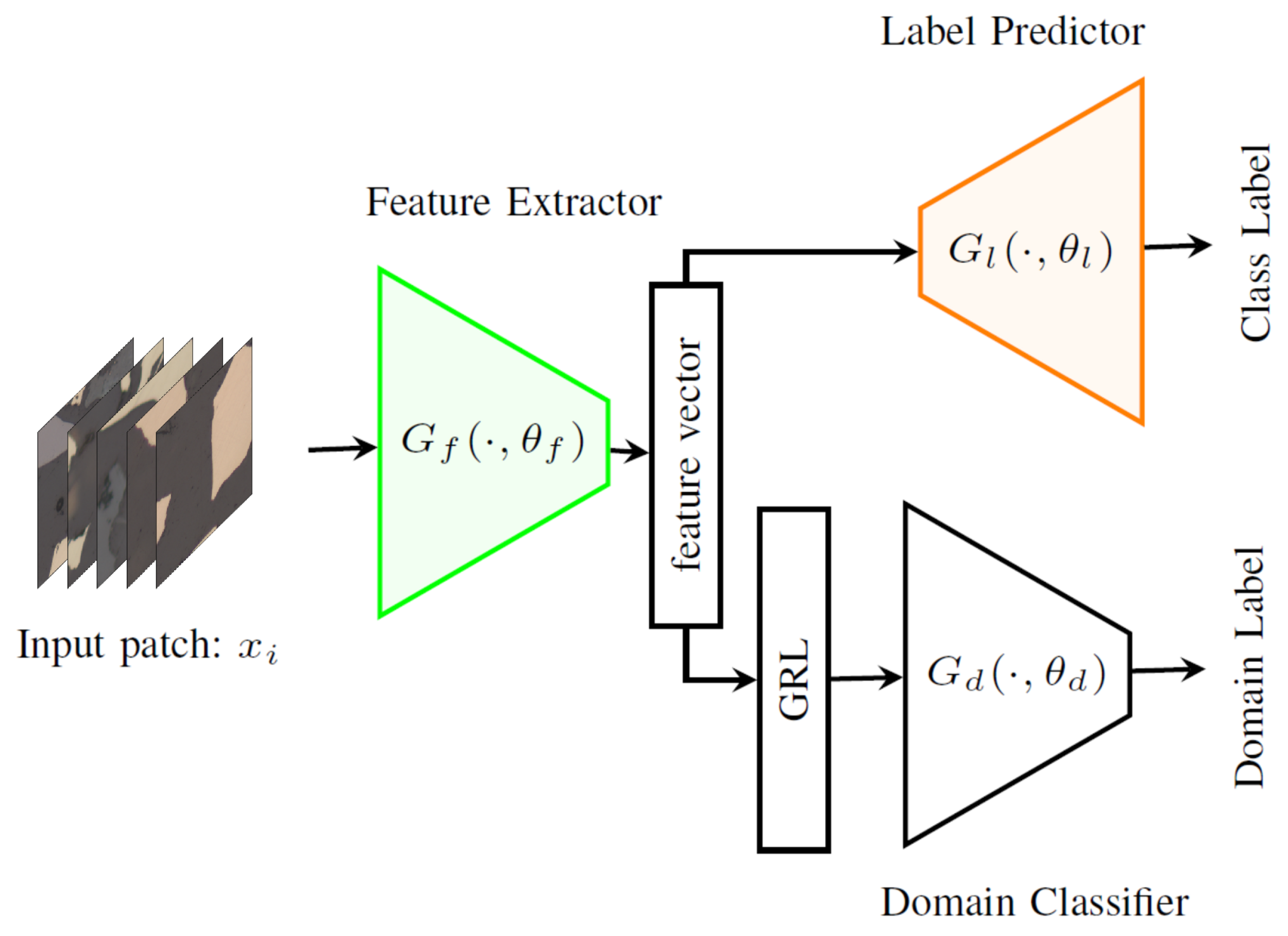
4.1. Domain Adversarial Neural Network (DANN)

Proposed in [7], DANN (Domain Adversarial Neural Network) consists of an adversarial training strategy aiming at producing a latent feature space, agnostic with respect to domains. Thus, its goal is to minimize the difference between the latent probability distributions of the source and target domains while projected to that feature space.

The architecture proposed in DANN is schematically represented by Figure 1. The neural networks assembly design consists of three modules: feature extractor; label predictor; and domain discriminator. The feature extractor $G_f(·,{\theta }_f)$ is a conventional CNN encoder which maps the features from the source and target domains into the common latent space. That single $G_f(·,{\theta }_f)$ function preforms simultaneous non-linear regression over ${}^{S}X$ and ${}^{T}X$ domains data, bringing about a latent feature space. The adversarial estimation of ${\theta }_f$ through out DANN training process is supposed to make that latent features space agnostic, so that the probabilities of source and target domains data, while projected on that space, fit to a common probability distribution, making $\mathrm{P}\left(G_f({}^{S}X,{\theta }_f)\right)\equiv \mathrm{P}\left(G_f({}^{T}X,{\theta }_f)\right)$.

The classifier $G_l(·,{\theta }_l)$, referred to as the label predictor, or decoder, classifies the input image based on its projection to the latent space. In the original DANN approach [7], the label predictor produces one label per input image. In contrast, on semantic segmentation problems like the one addressed in this study, this classification is done on the pixel level. Therefore, the herein presented classifier produces one label for each input image pixel.

The domain discriminator $G_d(·,{\theta }_d)$ is used during training to distinguish between latent features provided for samples of the source and target domains. In the course of the DANN training procedure, the domain discriminator competes with the feature extractor $G_f(·,{\theta }_f)$ aiming at motivating it to produce agnostic features. Nonetheless, we emphasize that in the training procedure proposed by DANN, since the true labels for the target domain samples are not available for training, gradients which reach to the encoder $G_f(·,{\theta }_f)$ are not influenced by the gradients originated by the flow of target samples through the label predictor. Anyway, features derived from both source and target domains are passed to the domain discriminator $G_d(·,{\theta }_d)$. That arrangement produces an adversarial scheme encompassing the feature extractor and the domain classifier. On the one hand, the feature extractor tends to produce agnostic features, while, on the other hand, that adversarial scheme leads the discriminator to learn to discern the origin of an image between source and target domains based on subtle features.

The objective function E to be optimized is defined by Equation (1), expressed as the sum of the losses of the classifier, represented by the first term of the equation, and the domain discriminator, represented by the second term. The term $R_{\lambda }\left(x\right)$ is described as a pseudo-function, defined by two mathematically incompatible equations, as shown in Equation (2).

$$E({\theta }_f,{\theta }_l,{\theta }_d)=\sum _{i;di=0}^N{L}_l(G_l(G_f(x_i,{\theta }_f),{\theta }_l),y_i)+\sum _i^N{L}_d(G_d(R_{\lambda }\left(G_f(x_i,{\theta }_f)\right),{\theta }_d),y_i)$$

(1)

$$\begin{array}{c}\hfill R_{\lambda }\left(x\right)=x\\ \\ \hfill {\displaystyle \frac{d{R}_{\lambda }}{dx}}=-\lambda \end{array}$$

(2)

The parameter $\lambda$ controls the influence of the gradients provided by domain discriminator in updating the encoder’s weights. Thus, the gradient of $L_d$ is used to update the weight values of the domain discriminator and the encoder in opposite directions, setting up the adversarial training scheme. In practice, this operation is implemented through a gradient reversal layer (GRL) positioned between the network’s encoder and the domain discriminator. The gradient reversal layer has no trainable parameters, and its function is merely to control the value of the gradients which are propagated back from the domain discriminator, acting as an identity function during network inference, but inverting the gradient value during the backpropagation process. Figure 1 schematically shows the gradient reversal layer positioned in the DANN structure.

During the training process, in order to obtain domain-invariant features, the parameters ${\theta }_f$ of the encoder are updated to maximize the loss of the domain discriminator. This effect means that the feature distributions are perfectly aligned, making it impossible for the discriminator to discern the origin domain of the sample. Simultaneously, the parameters of the domain discriminator are updated to minimize its loss. Thus, the encoder competes with the domain discriminator with opposing objectives. The optimization schemata for weights ${\theta }_f$, ${\theta }_l$ and ${\theta }_d$ are defined by equations (3), (4) and (5).

$${\theta }_f\leftarrow {\theta }_f-\mu \left({\displaystyle \frac{\partial L_l}{\partial {\theta }_f}}-\lambda {\displaystyle \frac{\partial L_d}{\partial {\theta }_f}}\right)$$

(3)

$${\theta }_l\leftarrow {\theta }_l-\mu {\displaystyle \frac{\partial L_l}{\partial {\theta }_l}}$$

(4)

$${\theta }_d\leftarrow {\theta }_d-\mu {\displaystyle \frac{\partial L_d}{\partial {\theta }_d}}$$

(5)

4.2. DeepLabv3+ Implementation

The DeepLab model family introduced a particular implementation of the hole algorithm [35], also known in DL terminology as atrous, or dilated convolution. Dilated convolutions have the ability of enlarging the field-of-view of traditional convolutional filters, incorporating larger spatial contexts without increasing the number of parameters or the amount of computations. In its next generation [36], the so-called atrous spatial pyramid pooling (ASPP) was introduced for capturing image contexts at multiple scales. Then, in the third generation of DeepLab [37], the original Conditional Random Fields (CRF) component was dropped out, and the ASPP component was extended incorporating image level features produced by an average pooling [38] that encodes global image context. Finally, the DeepLabv3+ model [39] adopts an encoder-decoder structure. The encoder follows the DeepLabv3 model while a simple but efficient decoder module was devised to enhance segmentation results especially along object boundaries.

The neural network architecture used in this work was inspired by [33], which corresponds to a variant of the original DeepLabv3+ architecture. The modifications of this work include the addition of dropout layers throughout the network and the replacement of the $8\times$ upsample with a $2\times$ upsample immediately at the network’s output. An illustration of the current DeepLabv3+ architecture is shown in the block diagram of Figure 2.

Dropout layers were added to prevent overfitting and enhance the network’s generalization capability, with all dropouts using a probability of $0.2$. In the original architecture used by [33], an $8\times$ upsample layer is used immediately before the softmax. However, preliminary tests indicated that such an abrupt interpolation complicates the classification of samples with large patch sizes. To address this issue, the $8\times$ upsample layer was replaced by a $2\times$ upsample layer to reduce the interpolation strength. This change required adjustments throughout the network by introducing an additional upsample layer positioned at the decoder input to properly scale the activations.

The output stride in fully convolutional networks like DeepLabv3+ controls the spatial dimensional reduction imposed to the activation maps which reach the network’s bottleneck. These differences are represented by the parameters A, B, and C presented with reddish letters in Figure 2. Parameter A denotes the stride value for an specific $1\times 1$ convolutional block in the encoder, assuming 1 for an output stride equal to 8, or 2 for an output stride equal to 16. The parameter B represents a function defined as a bypass $y=x$ for an output stride equal to 8 or a MaxPooling operation with a $2\times 2$ kernel and a stride of 2 for an output stride equal to 16. In the experiments reported in this work, we opted for an output stride of 16.

In the block diagram shown in Figure 2, the first parameter indicates the type of layer, the second parameter indicates the number of filters, the third parameter indicates the stride, and the last parameter indicates the dilation rate. For pooling layers, which do not have a dilation rate, the last parameter refers to the stride. The network’s bottleneck, a critical region where the activations are maximally reduced and discriminator is positioned, is located between the ASPP and the decoder. In Figure 2, the encoder is depicted by the green and blue blocks, while the decoder is represented by the dark orange block.

4.3. Discriminator Implementation

In the present DANN implementation, the domain discriminator consists of a fully connected network. Following [33], this network encompass two fully connected hidden layers containing 1024 neurons each and followed by ReLU activations. These layers are followed by an output layer containing two neurons with softmax activation layer. Table 1 provides a detailed description of the discriminator architecture.

4.4. Domain Datasets

The datasets used in this work are composed of pairs of correlated images, each pair contains one image acquired through reflected light microscopy, and the corresponding binary reference image, in which the pixels are labeled as belonging to one of two classes: embedding resin or ore particles. Correlative microscopy, also known as multimodal microscopy [40], was used to obtain properly registered images from a reflected light microscope and a SEM. The optical images were acquired at 24-bit RGB color quantization, and BSE images from SEM are 8-bit gray-level. Subsequently, the BSE images were processed using Fiji/ImageJ open source software [41] to generate the reference binary images. This annotation method, originally proposed by Filippo et al. [34], is objective and reproducible, avoiding the traditional and subjective method of producing reference images through manual delimitation and labeling.

In this study we did not consider errors arising from correlative microscopy (co-localization of fields and image registration) or due to image processing (delineation filtering and thresholding), as well as differences due to the distinct nature of the employed imaging techniques. For instance, images from reflected light microscopy and SEM come from different depths in the polished specimen, therefore these techniques may show ore particles differently if they are slightly under the polished surface. Nevertheless, in this study we assume that each reference image is considered as a correctly labeled image.

4.4.1. Fe19 dataset

This dataset contains images of an iron ore sample from the Serrote do Breu deposit (Brazil). Its mineralogy comprises quartz, magnetite, hematite, amphibole (hastingsite), albite, biotite, calcite, goethite, and kaolinite, with minor chlorite. Magnetite is the major iron mineral, followed by hematite, and rare goethite. The fraction +212–300 $\mu$m was cold mounted with epoxy resin and subsequently ground and polished. A total of 19 fields were imaged on a reflected light microscope with a 5×(NA 0.13) objective lens and on a SEM. Subsequently, the images from these different sensors were registered, resulting in image pairs of 972×972 pixels with a resolution of 2.17 $\mu$m/pixel. The complete description of this sample and its imaging procedure can be found in the work of Gomes et al. [42].

The images from SEM were then processed to compose the reference images. First, they were preprocessed with a delineation filter ($radius=1.5$ and $gradientthreshold=40$) [43] implemented as a Fiji macro, as described in [44]. The delineation (edge enhancement) converts gray-level ramps between phases in BSE images, the so-called halo effect, into sharp steps, so that the transition from one phase to the other occurs in a single pixel step. In sequence, the delineated images were thresholded: pixels with gray-levels between 0 and 80 were segmented as resin, and pixels with gray-levels above 80 were set as the ore particles.

4.4.2. Fe120 dataset

The images that compose this dataset came from the same epoxy embedding used to obtain the Fe19 dataset. However, despite it had been acquired with a experimental setup similar to Fe19, images of Fe120 dataset depicts a different cross-section. From such cross-section, 120 fields were imaged on a reflected light microscope with a 5×(NA 0.13) objective lens and on a SEM. Following, they were registered, resulting in images of 976×976 pixels with a resolution of 2.17 $\mu$m/pixel. Then, as described above, the images from SEM were processed to compose the reference images.

4.4.3. FeM dataset

This dataset was composed by images of an itabiritic iron ore concentrate from Quadrilátero Ferrífero (Brazil) mainly composed of hematite and quartz, with little magnetite and goethite. An ore sample was classified by size and concentrated with a dense liquid. Then, the sample +105–149 $\mu$m with density greater than 3.2 was cold mounted with epoxy resin and subsequently ground and polished. A total of 81 fields were imaged on a reflected light microscope with a 10×(NA 0.20) objective lens and on a SEM. In sequence, they were registered, resulting in images of 999×756 pixels with a resolution of 1.05 $\mu$m/pixel. The complete description of this sample and its imaging procedure can be found in the work of Gomes and Paciornik [45]. Finally, the images from SEM were thresholded to compose the reference images: pixels that have gray-levels between 0 and 70 were segmented as the resin, and pixels with gray-levels above 70 were set as the ore particles.

4.4.4. Cu dataset

This dataset contains images of a copper ore from Yauri Cusco (Peru) with a complex mineralogy, mainly composed of sulfides, oxides, silicates, and native copper. The ore was classified by size. The sample +74–100 $\mu$m was cold mounted with epoxy resin and subsequently ground and polished. A total of 121 fields were imaged on a reflected light microscope with a 20×(NA 0.40) objective lens and on a SEM. Following, they were registered, resulting in images of 1017×753 pixels with a resolution of 0.53 $\mu$m/pixel. The complete description of this sample and its imaging procedure can be found in the work of Gomes and Paciornik [46]. Finally, the images from SEM were thresholded to compose the reference images: pixels that have gray levels between 0 and 30 were segmented as the resin, and pixels with gray-levels above 30 were set as the ore particles.

4.4.5. Dataset Complexity

Concerning the results that will be presented in the following sections, we anticipate that the domain adaptation process exhibited different performances depending on the particular combinations of source and target domains. In order to provide some means to understand that behavior, we analyzed the complexity of each dataset.

We adopted the methodology employed in [4], where the number of clusters of a difference image (composed of channel-wise differences of images from different epochs) was used to describe domain complexity in the context of deforestation detection. We adapted methodology to the current context, and used the RGB intensities of the image pixels.

In the analysis, we computed the optimal number of clusters k considering all pixel locations of all images, for each domain, as shown in Table 2. To determine k, we executed the k-means algorithm a number of times and employed the Calinski-Harabasz criterion [47] for the different numbers of clusters in the respective domains. We observe that the number of clusters is associated with the diversity of patterns in the respective domains, thus indicating the complexity of different domains in terms of spectral variability.

According to the Calinski-Harabasz criterion, the Fe19 and Fe120 pixels optimally fitted to a total of 25 clusters, which is the highest value among the evaluated datasets, reflecting the largest number of phases, particularly non-opaque minerals, as shown in Section 4.4.1. On the other hand, the FeM database presented the smallest number of clusters in this evaluation, just 9 clusters, reflecting its simpler mineralogy, as it can be observed in Section 4.4.3. Furthermore, FeM contains images of an ore concentrate, unlike the other datasets, therefore it presents much less gangue minerals, as quartz and other non-opaque silicates.

4.5. Evaluation Metrics

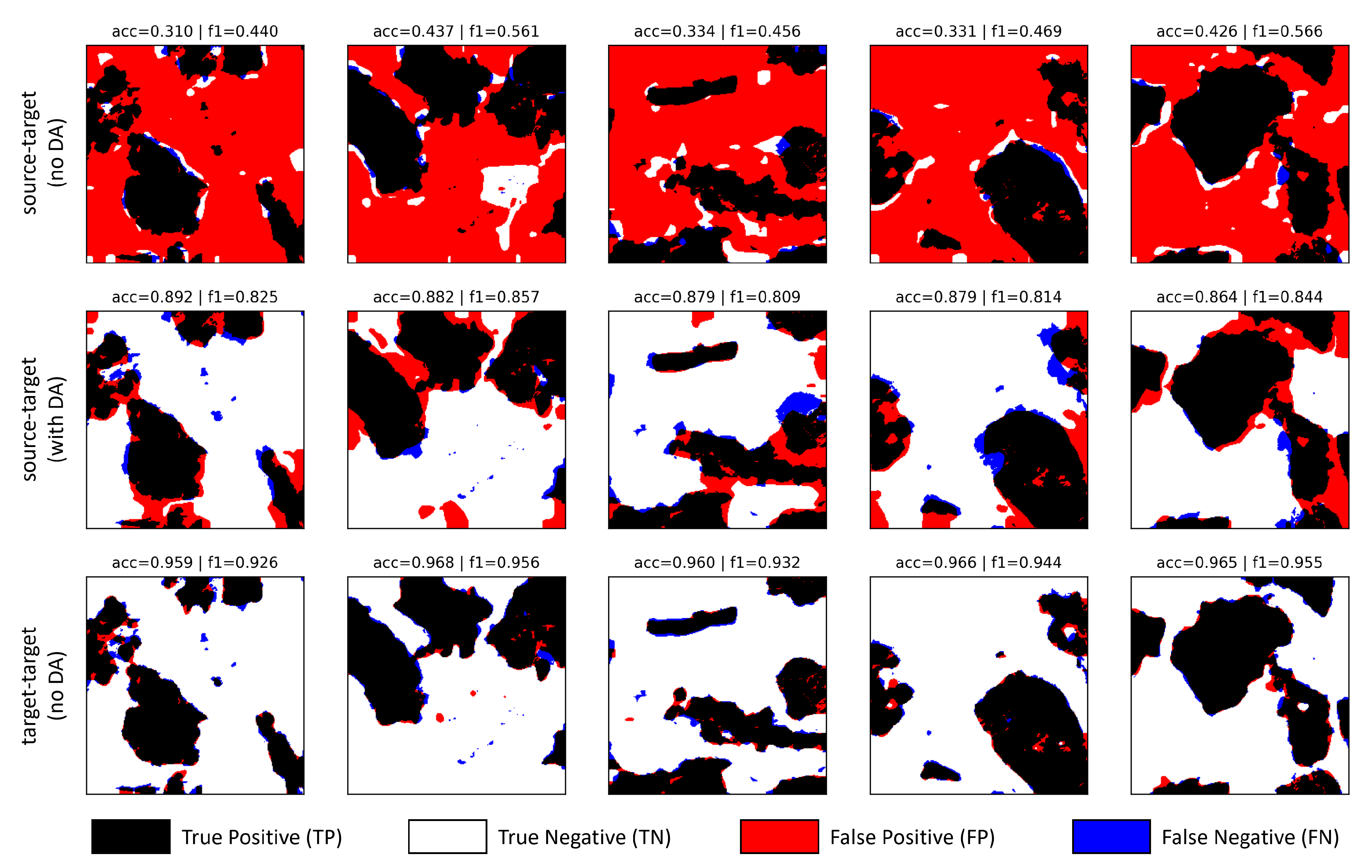
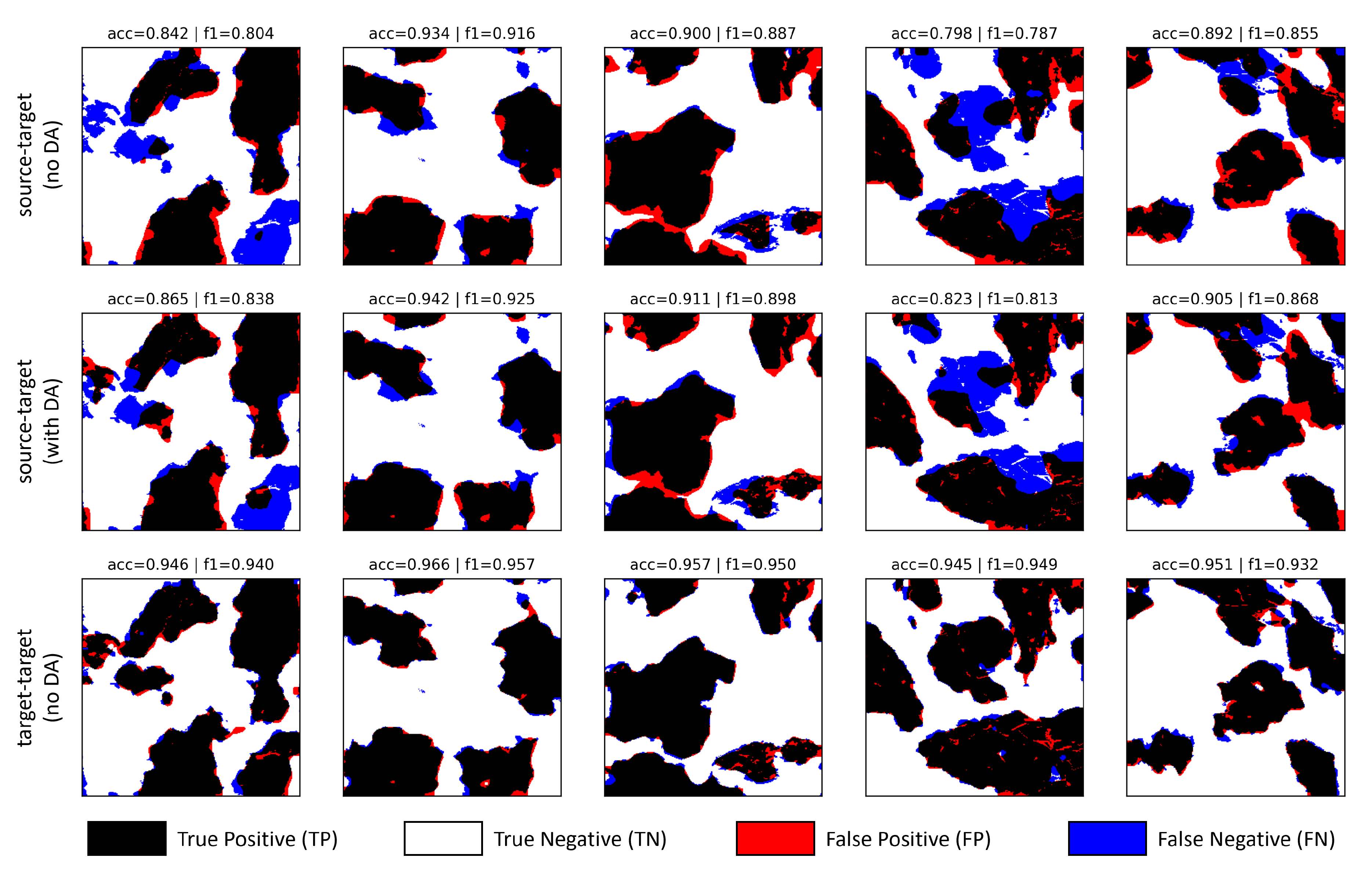
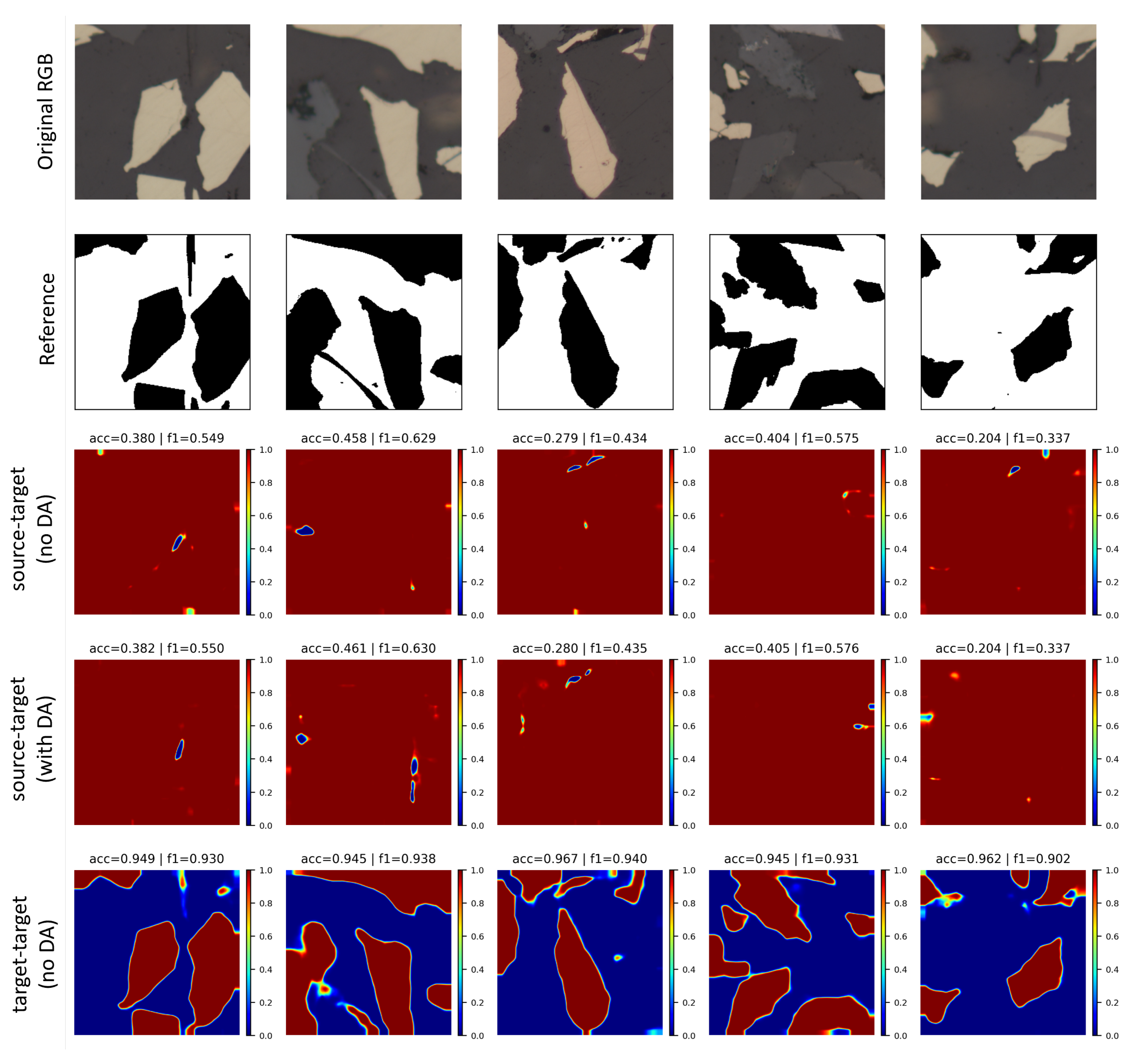
In this work, the assessment of the DL semantic segmentation is based on a number of metrics, namely: overall accuracy; precision; recall; F1-score; and average precision. These metrics are calculated based on the label predictor outcome. To calculate these metrics, each pixel of the semantic segmentation outcome is first assigned one of the following labels:

• True Positive ($TP$) - pixels correctly predicted as ore;
• False Positive ($FP$) - pixels predicted as ore, but should have been assigned to resin;
• True Negative ($TN$) - pixels correctly predicted as resin;
• False Negative ($FN$) - pixels predicted as resin, but should have been assigned to ore.

The descriptors that follow, which are derived from the $TP$, $TN$, $FP$ and $FN$ values, are used in the course of the experimental evaluation.

The overall accuracy ($OA$) measures the proportion of correct predictions in the outcome:

$$OA={\displaystyle \frac{TP+TN}{TP+FP+TN+FN}}·$$

(6)

Precision expresses the ratio between the number of true positives and the total of positive claims:

$$Precision={\displaystyle \frac{TP}{TP+FP}}·$$

(7)

Recall indicates the ratio between true positives and total number of positives in the reference:

$$Recall={\displaystyle \frac{TP}{TP+FN}}·$$

(8)

F1-score is the harmonic mean of the precision and recall metrics:

$$F1-score=2\times {\displaystyle \frac{Precision\times Recall}{Precision+Recall}}·$$

(9)

Several deep learning models, like the one herein exploited, uses softmax activations functions at the output layers. Such models present decision values between 0 and 1, representing for each pixel the probabilities of belonging to a certain group of classes. In general, the highest probability indicates the pixel class prediction. Given the decisions for an entire image, the ground truth image can then be applied for accounting TP, TN, FP and FN. In problems involving discriminating among two classes, however, is there an usual and more independent way of evaluating these metrics. The idea is to model the decisions as a function of the decision threshold value t. Distinct values of t, between 0 and 1, promote different TP, TN, FP and FN values, from which distinct values of precision and recall can be derived.

The average precision (AP) considers both precision and recall across different threshold levels. AP provides a single numerical value that summarizes the model’s performance over the threshold spectrum:

$$AP={\int }_0^{1}p\left(r\right)dr,$$

(10)

where $p\left(r\right)$ is a curve which plots the values of precision as a function of r, the recall values. The highest possible value of the AP is 1, indicating a result which agrees to the ground truth to all threshold t values in $[0,1]$.

5. Results and Discussion

We start this section by detailing the image data used in the experimental evaluation, obtained from each domain dataset presented in Section 4.4. Then, in order to guarantee experiments reproducibility, Section 5.2 contains a detailed description of the hyperparameters employed on the experimental setups. Finally, the experimental results are presented and discussed. First, in Section 5.3, we present cross-validation experiments, in which the DeepLabv3+ model was trained using data from a specific domain, and tested on the other domains. Considering the baseline and top-performing cross-validation results, Section 5.4 presents and discusses experiments using the DANN framework for different combinations of source and target domains.

5.1. Image Datasets

Table 3 presents the number of images available for each domain. The first column indicates the domain, the next column presents the total amount of images available, and the following columns indicate the number of images used for training, validation, and testing. The training and validation images numbers are shown together because training and validation patches are split on the course of the training cycle, just after data augmentation.

Before being processed by the DL models, the the intensity values in the RGB reflected light microscopy images were scaled to the range of $[0,1]$. From the resulting images, $256\times 256$ pixels patches were extracted, being these patches the actual inputs for the models.

The patches for training and validation were generated with a stride of 128, while the test patches were generated with a stride of 256, ensuring no overlap between them. The total number of patches for training, validation, and testing for each database is shown on Table 4. Two types of data augmentation were applied to the training and validation patches: rotation and flipping. The patches were rotated by ${90}^{\circ }$, ${180}^{\circ }$, and ${270}^{\circ }$. Flipping was performed along both the vertical and horizontal axes. Thus, the data augmentation operations added 5 patches for each originally available patch. Finally, the training and validation patches were divided respecting a 10% ratio for validation and the rest for training.

5.2. Experimental Parametrization

In all experiments the binary cross-entropy was used as loss function, for both the label predictor and domain discriminator of the DANN scheme (refer to Section 4.1 and Equation (1)). By and large, binary cross-entropy function summarizes the average difference between the real and predicted probabilities distributions for the positive class. The positive class, indicates ore in the case of the label predictor, and the source domain in the case of the domain discriminator. The binary cross entropy loss $\mathcal{L}$ formula is shown in Equation (11):

$$\mathcal{L}\left(\mathbf{x}\right)=-[y_{\mathbf{x}}\times logp\left(\mathbf{x}\right))+(1-y_{\mathbf{x}})\times log(1-p\left(\mathbf{x}\right))]·$$

(11)

When addressing the label predictor, $y_{\mathbf{x}}$ means the ground truth label for the input pixel $\mathbf{x}$, while $p\left(\mathbf{x}\right)$ is the predicted probability for that pixel $\mathbf{x}$ belonging to ore. Regarding the entire patch, the overall loss concerns the mean loss for all pixels in that patch. On the other hand, concerning the domain discriminator, since we have a single label per patch, $\mathbf{x}$ simply means an entire patch.

The optimizer used during training was Adam [48], an extension of the stochastic gradient descent (SGD) method, which relies on the adaptive estimation of first and second order momenta. This approach is computationally efficient, it has few memory requirements, and is invariant for the diagonal rescheduling of gradients. The parametrization of the optimizer was done following the recommendations suggested by [48]. Accordingly, the selected parameter values were set as ${\beta }_1$ equal to $0.9$; ${\beta }_2$ equal to $0.999$; and $ϵ$ equal to $1\times {10}^{-7}$.

The learning rate was empirically defined, as preliminary tests showed excellent results and satisfactory convergence at these levels. The learning rate calculation is defined by Equation 12:

$$\mu ={10}^{-(p+4)},$$

(12)

where p means the training progress, whose value varies linearly from zero, reaching one at the last training epoch.

Preliminary experiments revealed that in the current application, the gradients in the gradient reversal layer might explode, reaching very high values. To control the magnitude of the gradients that are backpropagated to the encoder, an additional parameter ${\lambda }_0$ was introduced in the original formulation prescribed in [7] for the computation of in Equation (3), as shown in Equation (13). The parameter ${\lambda }_0$ plays an essential role in the domain adaptation process, since it directly controls the magnitude of the gradients backpropagated to the network encoder. Therefore, the values of ${\lambda }_0$ must be fine-tuned for each experimental case.

$$\lambda ={\lambda }_0\times \left[{\displaystyle \frac{2}{(1+exp(-\gamma ·p\left)\right)}}-1\right]$$

(13)

In Equation (13), p is the training progress, having the same meaning as in Equation (12), while $\gamma =10$, in accordance with [7].

The weights of the network layers of all models were initialized randomly, following the uniform technique, described by [49].

The training procedure was programmed for lasting 100 epochs, with 25 epochs of patience for early stopping.

The experiments were carried out on a Ubuntu Linux operating system computer equipped with an Intel Xeon Silver 4214 processor and 128GB of RAM. The GPU used for DL models training was an 24GB NVIDIA GeForce RTX 4090.

5.3. Cross-Validation Experiments

As a practical evaluation for the original generalization ability of the DeepLabv3+ in the so-called cross-validation experiments, the model was trained with data from one domain and tested in all domains. The accuracy values presented in the following tables represent the average of five rounds of experiments. Standard deviation values for the exploited metrics obtained on these five rounds are indicated by the numbers in parentheses. The results are consistent with those presented in [34], although the implementations of the DeepLabv3+ architectures were slightly different.

According to the results, it is evident that all models performed very well when tested with samples from their own training set, achieving accuracy, precision, and recall values above 90%. However, when evaluated on datasets not used on training, the metrics exhibited consistently lower values, indicating the challenge of generalization. An exception was observed in the cross-validation with Fe19 and Fe120, as both datasets consist of images from the same ore sample, but acquired from different cross-sections. Furthermore, the metrics presented low dispersion among the five experiment rounds, as evidenced by the standard deviation values. This outcome suggests a consistent model performance.

Another interesting point to note is the asymmetry of the metrics. This means, for example, that a model trained on Fe19 and tested on Cu (Fe19-Cu) will not necessarily perform the same as a model trained on Cu and tested on Fe19 (Cu-Fe19). This effect is noticeable in the cases of FeM-Cu and Cu-FeM. The FeM-Cu case exhibited very low metrics, with accuracy and precision close to 35%, whereas the Cu-FeM case, while not achieving an ideal result, showed significantly higher metrics, with accuracy, precision, and recall close to 80%.

In fact, the model trained with the Cu dataset produced the highest overall cross-validation accuracy. Filippo et al. [34] suggested that this was due to the greater color variability of the optical images from the Cu dataset, which are quite colorful, while those of iron ores show mostly gray tones.

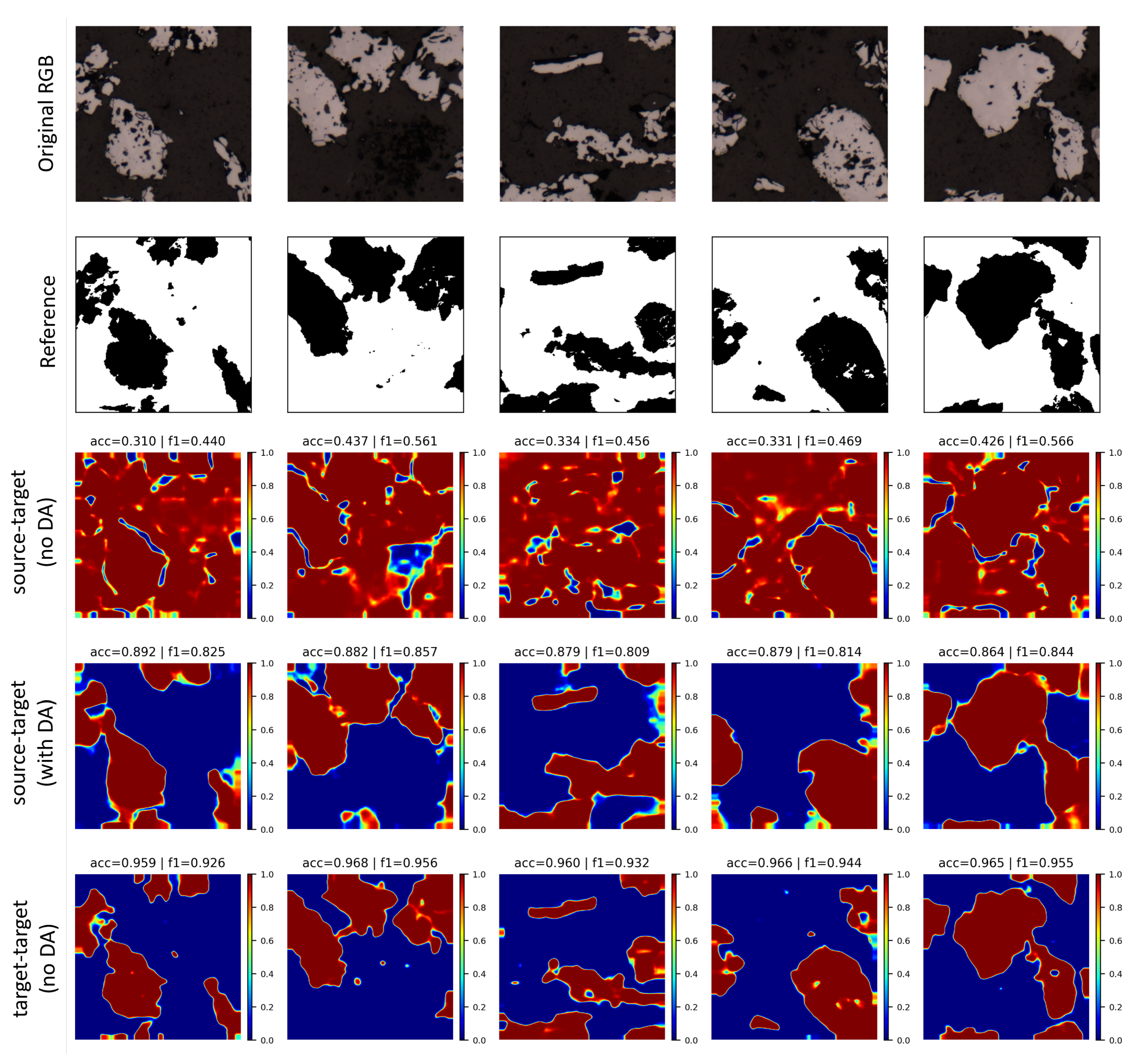
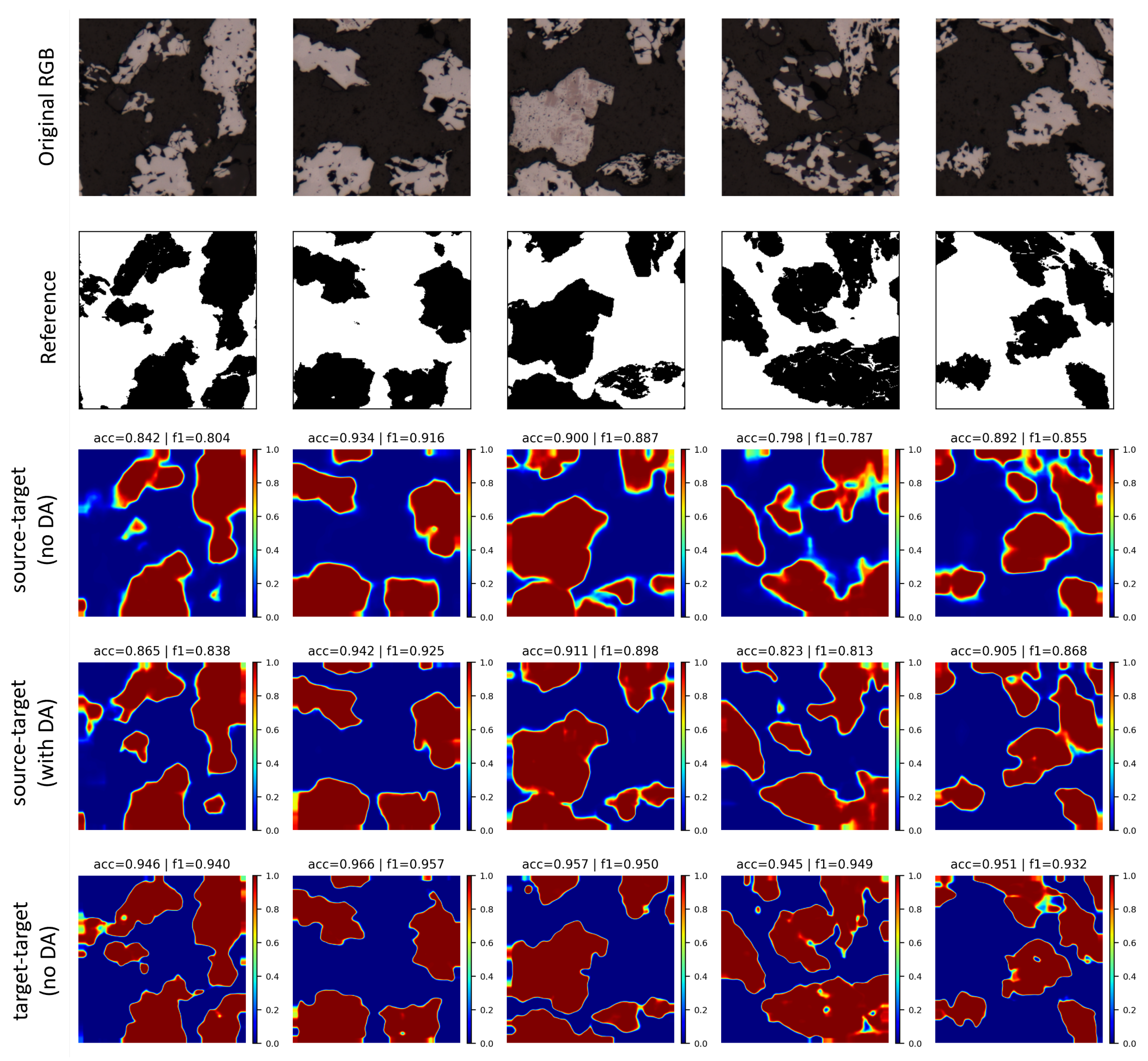
5.4. Domain Adaptation Experiments

Considering the structural similarities between the Fe19 and Fe120 databases described in Section 4.4.1 and Section 4.4.2 and the results presented in Section 5.3, the Fe19 and Fe120 databases can be considered as originate from the same domain. Therefore, for the sake of computational economy, we opted to discard the Fe120 database, during the DA experiments.

In the following experiments, a total of 500 patches from the source and target domains were randomly selected from the training patches mentioned in Table 4. These images were then subjected to the same data augmentation described in Section 5.1. As a consequence, a sum of 3,000 training images per domain are presented at each training epoch.

Another important issue considered is that controlling the training process is a challenge in DA. In a preliminary analysis, we observed numerical instabilities during training as the ${\lambda }_0$ value of the gradient reversal layer increased. These instabilities manifested as a sudden drop in the source domain classification accuracy, reaching bellow 5% in some cases. Consequently, it was necessary to adjust this hyperparameter to optimize model performance and, subsequently, the alignment of features during training.

During the investigation about the impact of the $\lambda$ parameter on model performance, three experiments rounds were run for each $\lambda$ value. Starting from $5\times {10}^{-6}$ and increasing its significant digits by increments in their values of one unit, a linear search for $\lambda$ was carried out. Afterwords, the optimal value of ${\lambda }_0$ was selected as the highest value at which none of the experiments exhibited the aforementioned drop in classification accuracy for the source domain.

Table 9 shows the ${\lambda }_0$ values for each source-target combination analyzed. According to the table, the lowest ${\lambda }_0$ value was $9\times {10}^{-6}$ for the FeM-Fe19 case, and the highest value was $1\times {10}^{-2}$ for the Cu-Fe19 case. In practice, most of the ${\lambda }_0$ values were on the order of ${10}^{-5}$, indicating a certain consistency in the definition of this hyperparameter.

Using the ${\lambda }_0$ values presented in Table 9, in a procedure analogous to that performed in the cross-domain experiments, five DA training rounds were carried out per source-target domain combination. DA results with our DeepLabv3+ implementation are present in Table 10, Table 11, Table 12, Table 13, Table 14 and Table 15 alongside cross-validation, and training on the target results, which respectively play the lower bound and upper bound roles in the DA performance evaluation. The columns of these tables present average values for accuracy, F1 score, average precision, and the linear performance gaps of these metrics computed for their respective averages. In such linear performance gap assessment, lower bounds are marked as 0% while the upper bound are assigned to 100%. The percentage for DA outcomes is linearly scaled in relation to that 0-100 range. The rows in these tables, on the other hand, reflect the results for different configurations with and without DA. The upper row presents results for a conventional cross-validation experiment using only training data of the source domain, and evaluated on the target domain test data. The bottom row presents the values for experiments training on the target data and testing also on target. These results are the same as previously presented in Table 5, Table 6, Table 7 and Table 8. The middle row presents the results for source-target DA.

Table 5. Cross-validation results provided by DeepLabv3+ trained on the Fe19 dataset.

Training set	Fe19
Test set	Fe19	Fe120	FeM	Cu
Accuracy	0.9175 (0.0086)	0.9251 (0.0055)	0.4354 (0.0154)	0.3548 (0.0003)
Precision	0.9148 (0.0153)	0.9225 (0.0103)	0.4048 (0.0066)	0.3538 (0.0001)
Recall	0.9287 (0.0036)	0.9348 (0.0072)	0.9757 (0.0096)	0.9989 (0.0007)
F1 score	0.9216 (0.0069)	0.9285 (0.0035)	0.5721 (0.0070)	0.5225 (0.0001)
Avg. precision	0.9753 (0.0066)	0.9804 (0.0032)	0.8213 (0.0194)	0.6085 (0.2050)

Table 5. Cross-validation results provided by DeepLabv3+ trained on the Fe19 dataset.

Training set	Fe19
Test set	Fe19	Fe120	FeM	Cu
Accuracy	0.9175 (0.0086)	0.9251 (0.0055)	0.4354 (0.0154)	0.3548 (0.0003)
Precision	0.9148 (0.0153)	0.9225 (0.0103)	0.4048 (0.0066)	0.3538 (0.0001)
Recall	0.9287 (0.0036)	0.9348 (0.0072)	0.9757 (0.0096)	0.9989 (0.0007)
F1 score	0.9216 (0.0069)	0.9285 (0.0035)	0.5721 (0.0070)	0.5225 (0.0001)
Avg. precision	0.9753 (0.0066)	0.9804 (0.0032)	0.8213 (0.0194)	0.6085 (0.2050)

Table 6. Cross-validation results provided by DeepLabv3+ trained on the Fe120 dataset.

Training set	Fe120
Test set	Fe19	Fe120	FeM	Cu
Accuracy	0.9258 (0.0063)	0.9345 (0.0092)	0.4861 (0.0380)	0.4073 (0.1017)
Precision	0.9266 (0.0080)	0.9375 (0.0088)	0.4282 (0.0189)	0.3783 (0.0481)
Recall	0.9327 (0.0037)	0.9398 (0.0087)	0.9666 (0.0099)	0.9876 (0.0202)
F1 score	0.9296 (0.0056)	0.9386 (0.0081)	0.5932 (0.0177)	0.5447 (0.0438)
Avg. precision	0.9809 (0.0034)	0.9867 (0.0030)	0.8618 (0.0181)	0.8064 (0.0837)

Table 6. Cross-validation results provided by DeepLabv3+ trained on the Fe120 dataset.

Training set	Fe120
Test set	Fe19	Fe120	FeM	Cu
Accuracy	0.9258 (0.0063)	0.9345 (0.0092)	0.4861 (0.0380)	0.4073 (0.1017)
Precision	0.9266 (0.0080)	0.9375 (0.0088)	0.4282 (0.0189)	0.3783 (0.0481)
Recall	0.9327 (0.0037)	0.9398 (0.0087)	0.9666 (0.0099)	0.9876 (0.0202)
F1 score	0.9296 (0.0056)	0.9386 (0.0081)	0.5932 (0.0177)	0.5447 (0.0438)
Avg. precision	0.9809 (0.0034)	0.9867 (0.0030)	0.8618 (0.0181)	0.8064 (0.0837)

Table 7. Cross-validation results provided by DeepLabv3+ trained on the FeM dataset.

Training set	FeM
Test set	Fe19	Fe120	FeM	Cu
Accuracy	0.5199 (0.0026)	0.5270 (0.0162)	0.9557 (0.0010)	0.3534 (0.0001)
Precision	0.5249 (0.0028)	0.5295 (0.0151)	0.9467 (0.0033)	0.3534 (0.0000)
Recall	0.9748 (0.0111)	0.9824 (0.0151)	0.9384 (0.0036)	0.9999 (0.0001)
F1 score	0.6823 (0.0025)	0.6881 (0.0162)	0.9425 (0.0014)	0.5222 (0.0001)
Avg. precision	0.6255 (0.0929)	0.6228 (0.0873)	0.9884 (0.0004)	0.4940 (0.1976)

Table 7. Cross-validation results provided by DeepLabv3+ trained on the FeM dataset.

Training set	FeM
Test set	Fe19	Fe120	FeM	Cu
Accuracy	0.5199 (0.0026)	0.5270 (0.0162)	0.9557 (0.0010)	0.3534 (0.0001)
Precision	0.5249 (0.0028)	0.5295 (0.0151)	0.9467 (0.0033)	0.3534 (0.0000)
Recall	0.9748 (0.0111)	0.9824 (0.0151)	0.9384 (0.0036)	0.9999 (0.0001)
F1 score	0.6823 (0.0025)	0.6881 (0.0162)	0.9425 (0.0014)	0.5222 (0.0001)
Avg. precision	0.6255 (0.0929)	0.6228 (0.0873)	0.9884 (0.0004)	0.4940 (0.1976)

Table 8. Cross-validation results provided by DeepLabv3+ trained on the Cu dataset.

Training set	Cu
Test set	Fe19	Fe120	FeM	Cu
Accuracy	0.7033 (0.0233)	0.7110 (0.0189)	0.8894 (0.0060)	0.9388 (0.0026)
Precision	0.8936 (0.0246)	0.8960 (0.0223)	0.8666 (0.0190)	0.9380 (0.0067)
Recall	0.4759 (0.0368)	0.5131 (0.0265)	0.8448 (0.0132)	0.8855 (0.0096)
F1 score	0.6204 (0.0349)	0.6522 (0.0256)	0.8553 (0.0064)	0.9109 (0.0040)
Avg. precision	0.8015 (0.0368)	0.8201 (0.0335)	0.9284 (0.0032)	0.9678 (0.0011)

Table 8. Cross-validation results provided by DeepLabv3+ trained on the Cu dataset.

Training set	Cu
Test set	Fe19	Fe120	FeM	Cu
Accuracy	0.7033 (0.0233)	0.7110 (0.0189)	0.8894 (0.0060)	0.9388 (0.0026)
Precision	0.8936 (0.0246)	0.8960 (0.0223)	0.8666 (0.0190)	0.9380 (0.0067)
Recall	0.4759 (0.0368)	0.5131 (0.0265)	0.8448 (0.0132)	0.8855 (0.0096)
F1 score	0.6204 (0.0349)	0.6522 (0.0256)	0.8553 (0.0064)	0.9109 (0.0040)
Avg. precision	0.8015 (0.0368)	0.8201 (0.0335)	0.9284 (0.0032)	0.9678 (0.0011)

Table 9. Values of ${\lambda }_0$ for each source-target combination.

Source	Target	${\mathit{\lambda }}_0$
Fe19	FeM	$2·{10}^{-5}$
Fe19	Cu	$1·{10}^{-5}$
FeM	Fe19	$9·{10}^{-6}$
FeM	Cu	$1·{10}^{-5}$
Cu	Fe19	$1·{10}^{-2}$
Cu	FeM	$4·{10}^{-5}$

Table 9. Values of ${\lambda }_0$ for each source-target combination.

Source	Target	${\mathit{\lambda }}_0$
Fe19	FeM	$2·{10}^{-5}$
Fe19	Cu	$1·{10}^{-5}$
FeM	Fe19	$9·{10}^{-6}$
FeM	Cu	$1·{10}^{-5}$
Cu	Fe19	$1·{10}^{-2}$
Cu	FeM	$4·{10}^{-5}$

Table 10. Domain adaptation results for the domain combination source-target: Fe19-FeM.

	Metrics			Performance Gap
	Accuracy	F1	AP	Accuracy [%]	F1 [%]	AP [%]
source-target (no DA)	0.4405	0.5713	0.7241	0.0	0.0	0.0
source-target (DA)	0.7079	0.7118	0.8007	52.35	38.41	29.29
target-target (no DA)	0.9513	0.9369	0.9856	100.0	100.0	100.0

Table 10. Domain adaptation results for the domain combination source-target: Fe19-FeM.

	Metrics			Performance Gap
	Accuracy	F1	AP	Accuracy [%]	F1 [%]	AP [%]
source-target (no DA)	0.4405	0.5713	0.7241	0.0	0.0	0.0
source-target (DA)	0.7079	0.7118	0.8007	52.35	38.41	29.29
target-target (no DA)	0.9513	0.9369	0.9856	100.0	100.0	100.0

Table 11. Domain adaptation results for the domain combination source-target: Fe19-Cu

	Metrics			Performance Gap
	Accuracy	F1	AP	Accuracy [%]	F1 [%]	AP [%]
source-target (no DA)	0.3556	0.5227	0.4781	0.0	0.0	0.0
source-target (DA)	0.4009	0.5315	0.4749	7.743	2.248	-0.6612
target-target (no DA)	0.9419	0.9153	0.9707	100.0	100.0	100.0

Table 11. Domain adaptation results for the domain combination source-target: Fe19-Cu

	Metrics			Performance Gap
	Accuracy	F1	AP	Accuracy [%]	F1 [%]	AP [%]
source-target (no DA)	0.3556	0.5227	0.4781	0.0	0.0	0.0
source-target (DA)	0.4009	0.5315	0.4749	7.743	2.248	-0.6612
target-target (no DA)	0.9419	0.9153	0.9707	100.0	100.0	100.0

Table 12. Domain adaptation results for the domain combination source-target: FeM-Fe19.

	Metrics			Performance Gap
	Accuracy	F1	AP	Accuracy [%]	F1 [%]	AP [%]
source-target (no DA)	0.5414	0.6648	0.6898	0.0	0.0	0.0
source-target (DA)	0.5469	0.6688	0.6984	1.454	1.464	3.008
target-target (no DA)	0.9181	0.9395	0.9750	100.0	100.0	100.0

Table 12. Domain adaptation results for the domain combination source-target: FeM-Fe19.

	Metrics			Performance Gap
	Accuracy	F1	AP	Accuracy [%]	F1 [%]	AP [%]
source-target (no DA)	0.5414	0.6648	0.6898	0.0	0.0	0.0
source-target (DA)	0.5469	0.6688	0.6984	1.454	1.464	3.008
target-target (no DA)	0.9181	0.9395	0.9750	100.0	100.0	100.0

Table 13. Domain adaptation results for the domain combination source-target: FeM-Cu.

	Metrics			Performance Gap
	Accuracy	F1	AP	Accuracy [%]	F1 [%]	AP [%]
source-target (no DA)	0.3576	0.5237	0.6254	0.0	0.0	0.0
source-target (DA)	0.3534	0.5222	0.6771	-0.7228	-0.3755	14.96
target-target (no DA)	0.9419	0.9153	0.9707	100.0	100.0	100.0

Table 13. Domain adaptation results for the domain combination source-target: FeM-Cu.

	Metrics			Performance Gap
	Accuracy	F1	AP	Accuracy [%]	F1 [%]	AP [%]
source-target (no DA)	0.3576	0.5237	0.6254	0.0	0.0	0.0
source-target (DA)	0.3534	0.5222	0.6771	-0.7228	-0.3755	14.96
target-target (no DA)	0.9419	0.9153	0.9707	100.0	100.0	100.0

Table 14. Domain adaptation results for the domain combination source-target: Cu-Fe19.

	Metrics			Performance Gap
	Accuracy	F1	AP	Accuracy [%]	F1 [%]	AP [%]
source-target (no DA)	0.6962	0.6057	0.7889	0.0	0.0	0.0
source-target (DA)	0.7032	0.6286	0.7957	2.871	7.393	3.762
target-target (no DA)	0.9181	0.9395	0.9750	100.0	100.0	100.0

Table 14. Domain adaptation results for the domain combination source-target: Cu-Fe19.

	Metrics			Performance Gap
	Accuracy	F1	AP	Accuracy [%]	F1 [%]	AP [%]
source-target (no DA)	0.6962	0.6057	0.7889	0.0	0.0	0.0
source-target (DA)	0.7032	0.6286	0.7957	2.871	7.393	3.762
target-target (no DA)	0.9181	0.9395	0.9750	100.0	100.0	100.0

Table 15. Domain adaptation results for the domain combination source-target: Cu-FeM.

	Metrics			Performance Gap
	Accuracy	F1	AP	Accuracy [%]	F1 [%]	AP [%]
source-target (no DA)	0.8518	0.7887	0.8809	0.0	0.0	0.0
source-target (DA)	0.8760	0.8380	0.9133	24.32	33.25	30.97
target-target (no DA)	0.9513	0.9369	0.9856	100.0	100.0	100.0

Table 15. Domain adaptation results for the domain combination source-target: Cu-FeM.

	Metrics			Performance Gap
	Accuracy	F1	AP	Accuracy [%]	F1 [%]	AP [%]
source-target (no DA)	0.8518	0.7887	0.8809	0.0	0.0	0.0
source-target (DA)	0.8760	0.8380	0.9133	24.32	33.25	30.97
target-target (no DA)	0.9513	0.9369	0.9856	100.0	100.0	100.0

The cases with the most evident domain adaptation were Fe19-FeM and Cu-FeM. In the Fe19-FeM case exhibited in Table 10, approximately 52%, 38%, and 29% of the performance gaps in accuracy, F1 score, and average precision, respectively, were filled. In the Cu-FeM case presented in Table 15, around 24%, 33%, and 31% of the performance gaps in the same metrics were recorded. Although the performance gap fillings are higher in the Fe19-FeM case, it is important to emphasize that the baseline accuracy value for the Cu-FeM case is higher (85%), making any performance gain substantially more challenging due to a narrower domain gap between the source and target domains. Conversely, in the Fe19-FeM case, the baseline accuracy value may be considered low (44%), providing the model with a much larger margin for performance improvement when domain adaptation is performed.

Regarding the domain combinations outcomes exploiting FeM database as source, both performed poorly. In the FeM-Cu case denoted by Table 13, the performance gap fillings for accuracy and F1 score were negligible. Both values were negative but with small absolute values, suggesting minimal influence of domain adaptation on these metrics. However, the average precision stood out with a performance gap filling of approximately 15%. This observation may indicate that domain adaptation in this case might have affected the probability threshold regulation, suggesting that domain adaptation can manifest in different ways and have varied impacts on the model’s performance. In the FeM-Fe19 evaluation depicted by Table 12, accuracy and F1 scores were significantly poor, showing small positive values.

An asymmetry in the metrics was also observed with respect to homologous source-target combinations. Comparing the outcomes for Fe19-Cu and Cu-Fe19 combinations presented in Table 11 and Table 14, it is possible noticing an intrinsic asymmetry between baseline values for F1 score, for instance, which presented approximately 0.52 for Fe19-Cu and 0.6 for Cu-Fe19. Concerning the F1 score performance gaps filled by DA for such combinations, one can notice that for Fe19-Cu 2.2% was filled, while for the Cu-Fe19 7.4% of the performance gap was filled.

The same discrepancies are present in FeM-Cu and Cu-FeM combinations, which presented approximate baseline values for F1 score of 0.52 and 0.79, see Table 13 and Table 15. Addressing the F1 score performance gaps provided by DA, it can be seen that for the Fe19-Cu combination domain adaptation led to a 3.7% worsening in performance. Nonetheless, while for Cu-FeM DA was able to fill more than 33% of the F1 score performance gap.

Regarding the Fe19-FeM and FeM-Fe19 experimental results presented in Table 10 and Table 12 respectively, F1 score values for the baseline outcomes were around 0.57 and 0.66. Addressing the F1 score performance gaps reduction provided by DA, it can be seen that for the Fe19-FeM combination the domain adaptation led to fill 38.7% of the performance gap. For the FeM-Fe19 combination, however, less than 1.5% was filled.

Another important aspect to be conjectured concerns what domain features may lead to a positive and significant DA contribution. Observing the previously presented results, one can notice that the use of FeM as source domain provided systematically poor results. However, on the other hand, when the FeM database takes on the role of target domain, the results show undeniably positive metrics. DA results combining Fe19 and Cu as source and target indistinctly were positive, however, with a small absolute improvement values. The examination of Table 2 may bring some important elements to this evaluation. According to the variability metrics presented in Table 2, Fe19 is the most complex domain, since the set of pixels of this domain fits to 25 clusters according to k-means algorithm and the Calinski-Harabasz criterion. The Cu domain dataset, in turn, fitted to 15 clusters, while the FeM database fitted to only 9 clusters.

Taking into account the values observed in Table 2 and the results presented in Table 10, Table 11, Table 12, Table 13, Table 14 and Table 15, some preliminary hypotheses could be raised for explaining the results obtained in the present research. The first is that there needs to be a certain fit between the characteristics and complexity of the source and target domains. This may partially explain the method’s poor performance in certain combinations. Secondly, these domain combinations should privilege combinations in which the source domain presents more variability than the target domain. That perhaps be the reason why having the FeM as target provided a consistent DA result of high magnitude. Besides, it may explain why using FeM as source domain was so unsuccessful.

It’s important to emphasize that the relationship between classifier performance and complexity is consistent with the findings presented in [4], using k-means in conjunction with the Calinski-Harabasz criterion. Although the target application discussed in [4] differs from the one explored in this study, the domain complexity measure has been used to provide a more objective explanation of classifier performance when trained and tested within specific domains. The results of domain adaptation, particularly those indicating negative transfer — such as the case of FeM-Cu (Table 13) — can be partially understood through this perspective on complexity. Specifically, as shown in Table 2, FeM represents the domain with the lowest spectral variability according to the number of clusters found.

In the remaining of this section a qualitative assessment of the DA results is provided for the two more successful combinations of source target domains: Fe19-FeM and Cu-FeM. Figure 3 presents a $5\times 5$ grid concerning OS 16 models, in which columns represent the results for a patch randomly selected from the target domain. The first row of each grid displays the RGB optical microscopy images of the selected input patches. The second row shows the reference ground truth data. Rows 3, 4 and 5 concern probabilities maps provided by a DeepLabv3+ model randomly selected among the five available trained models. Notice the numbers on the top of each probability map which express the accuracy and F1 scores values provided by the respective model for that given target patch. Specifically, the third row presents the baseline result – source-target model (without DA) – corresponding to DeepLabv3+ models conventionally trained based on the source domain training data and tested on the target domain. The fourth row shows the probability results from the DA source-target model trained with the DANN method. The final row displays the probability results from the upper bound result – the target-target model (without DA) –, concerning a DeepLabv3+ model trained using target training data.

Results present in Figure 3 reveal that the baseline model failed to adequately identify resin pixels, classifying most of the image as ore. However, with domain adaptation, the model was able to accurately delineate the ore particles and the resin region. Despite this improvement, the particle edges appeared overly rounded, lacking geometric refinement.

This lack of edge refinement is confirmed in Figure 4, which shows the classification results using a 50% probability threshold. According to the color legend, black means TP, white pixels refer to TN, red express FP, while blue indicates FN. It is evident that the model trained with the DANN method produces a significant number of false positives along the edges and in narrow regions between particles, causing them to merge with each other. The fact that the reference images were derived from SEM images may have contributed to the concentration of errors at the particle edges, since the reflected light microscopy images and the labels originated from different sources and relate to different sample depths.

The image in Figure 5 shows the probability maps for the Cu-FeM case, where domain adaptation also yielded satisfactory results, although less evident, as indicated in Table 15. In this case, the baseline model produced a relatively acceptable result with approximately 82% accuracy, suggesting a narrow domain gap. It can also be observed that in the baseline model, the ore particle edges have a wider region of intermediate probabilities close to 50%. The use of the DANN method successfully refined these edges and reduced the width of such regions.

The image in Figure 6 shows that the baseline model generated an excessively high number of false negatives, clustered in blue, which represent ore particles classified as resin. Domain adaptation achieved a slight refinement of these clusters, resulting in a modest increase in performance metrics. However, a significant portion of these particles remained undetected.

The image in Figure 7 displays the probability maps for the Fe19-Cu domain combination, where the results of domain adaptation were unsatisfactory, as indicated in Table 11. Almost the entire image was classified by the baseline model as ore particles. In this case, domain adaptation did not provide any visible benefit for image inference, with classification metrics remaining practically unchanged.

6. Conclusions

The present work concerns the discrimination of opaque and non-opaque minerals from the embedding epoxy resin in reflected light microscopy images. The major difficulty in such a classical ore microscopy problem arises from the spectral similarity, in terms of specular reflectance, between non-opaque minerals and the embedding resin. In this application, conventional deep learning semantic segmentation approaches have been performing consistently well on data from the same image domain, from which they were trained on. However, in general, they struggle with cross-domain generalization.

This limitation became clear in the cross-validation experiments using DeepLabv3+ model implemented in this research, with few exceptions, such as when trained with the Cu dataset and tested on data from the FeM dataset, which displayed relatively high accuracy. Those results motivated the engagement regarding the evaluation of domain adaptation to this application. Domain adaptation is an emerging topic in computer vision, and has come to compensate for the loss of performance caused by domain shifts in cross-domains situations.

Another important point which arose in this experimental evaluation is that the models showed an asymmetry in generalization ability. For instance, a model trained in the Cu dataset and evaluated on FeM dataset data does not necessarily perform similarly when trained with the FeM data and tested with the Cu. This trend was observed across all experiments. Those experimental results provided over five independent trials for each setup showed low standard deviation, indicating the robustness and consistency of the models even when they performed poorly. Consequently, we believe that asymmetry is due to some intrinsic inter-domains issue. Thus, compatibility between the structural complexities of the source and the target domains needs to be respected with special attention. Therefore, in principle, based on the evidence gathered here, it is necessary to create a strategy in which the complexity of the target domain can be received by the characteristics constructed for the classification of the source domain. Better controlling that compatibility is an important issue to be addressed in future works.

Domain adaptation presents significant challenges due to the large number of hyperparameters and their specific effects on classification performance. Optimizing these models requires an extensive search for the right hyperparameters space. Though, this process is computationally expensive and demands efficient search strategies.

Domain adaptation proved to be effective in some source-target combinations, although not for all cases. In particular, notable performance improvements were observed using the FeM database as target while either Fe19 or Cu databases could indistinctly assume the role of source domain. This bring attention to fact that domain adaptation for semantic segmentation can be a pathway for research in the ore characterization field. The increase in generalization capacity of DL models for the semantic segmentation of minerals in reflected light microscopy images opens up possibilities for developing automated mineralogy solutions based on this microscopy technique. This is of great interest for the mining industry due to its ability to identify minerals and its lower cost compared to SEM-based systems.

Besides, the suggestions provided in this conclusion, readers may notice other research opportunities for domain adaptation not listed in this section and that also may come about in the exploitation of other applications.

References

1. Gomes, O.d.F.M.; Iglesias, J.C.A.; Paciornik, S.; Vieira, M.B. Classification of hematite types in iron ores through circularly polarized light microscopy and image analysis. Minerals Engineering 2013, 52, 191–197. [Google Scholar] [CrossRef]
2. Neumann, R.; Stanley, C.J. Specular reflectance data for quartz and some epoxy resins: implications for digital image analysis based on reflected light optical microscopy. Ninth International Congress for Applied Mineralogy, 2008, pp. 703–705.
3. Wang, M.; Deng, W. Deep visual domain adaptation: A survey. Neurocomputing 2018, 312, 135–153. [Google Scholar] [CrossRef]
4. Vega, P.J.S.; da Costa, G.A.O.P.; Feitosa, R.Q.; Adarme, M.X.O.; de Almeida, C.A.; Heipke, C.; Rottensteiner, F. An unsupervised domain adaptation approach for change detection and its application to deforestation mapping in tropical biomes. ISPRS Journal of Photogrammetry and Remote Sensing 2021, 181, 113–128. [Google Scholar] [CrossRef]
5. Wittich, D.; Rottensteiner, F. Wittich, D.; Rottensteiner, F. Appearance Based Deep Domain Adaptation for the Classification of Aerial Images. CoRR 2021, abs/2108.07779. [CrossRef]
6. Le, T.; Nguyen, T.; Ho, N.; Bui, H.; Phung, D. LAMDA: Label Matching Deep Domain Adaptation. Proceedings of Machine Learning Research 2021, 139, 6043–6054. [Google Scholar]
7. Ganin, Y.; Lempitsky, V. Unsupervised domain adaptation by backpropagation. Skoltech 2014. [Google Scholar] [CrossRef]
8. Pan, S.J.; Yang, Q. A Survey on Transfer Learning. IEEE Transactions on Knowledge and Data Engineering 2010, 22, 1345–1359. [Google Scholar] [CrossRef]
9. Tuia, D.; Persello, C.; Bruzzone, L. Domain Adaptation for the Classification of Remote Sensing Data: An Overview of Recent Advances. IEEE Geoscience and Remote Sensing Magazine 2016, 4, 41–57. [Google Scholar] [CrossRef]
10. Weiss, K.; Khoshgoftaar, T.; Wang, D. A survey of transfer learning. J Big Data 2016, 3, 40. [Google Scholar] [CrossRef]
11. Csurka, G. A comprehensive survey on domain adaptation for visual applications. In Domain Adaptation in Computer Vision Applications, 1 ed.; Csurka, G., Ed.; Springer: Cham, 2017; Vol. 1, Advances in Computer Vision and Pattern Recognition, chapter 1, pp. 1–35. [Google Scholar] [CrossRef]
12. Wilson, G.; Cook, D.J. A Survey of Unsupervised Deep Domain Adaptation. ACM Trans. Intell. Syst. Technol. 2020, 11, 1–46. [Google Scholar] [CrossRef] [PubMed]
13. Masci, J.; Meier, U.; Ciresan, D.; Schmidhuber, J.; Fricout, G. Steel defect classification with Max-Pooling Convolutional Neural Networks. The 2012 International Joint Conference on Neural Networks (IJCNN), 2012, pp. 1–6. [CrossRef]
14. Jiang, F.; Gu, Q.; Hao, H.; Li, N. Feature Extraction and Grain Segmentation of Sandstone Images Based on Convolutional Neural Networks. 2018 24th International Conference on Pattern Recognition (ICPR), 2018, pp. 2636–2641. [CrossRef]
15. Liu, X.; Zhang, Y.; Jing, H.; Wang, L.; Zhao, S. Ore image segmentation method using U-Net and Res_Unet convolutional networks. RSC Adv. 2020, 10, 9396–9406. [Google Scholar] [CrossRef]
16. Svensson, T. Semantic Segmentation of Iron Ore Pellets with Neural Networks. Master’s thesis, Luleå University of Technology, Department of Computer Science, Electrical and Space Engineering, 2019.
17. Lorenzoni, R.; Curosu, I.; Paciornik, S.; Mechtcherine, V.; Oppermann, M.; Silva, F. Semantic segmentation of the micro-structure of strain-hardening cement-based composites (SHCC) by applying deep learning on micro-computed tomography scans. Cement and Concrete Composites 2020, 108, 103551. [Google Scholar] [CrossRef]
18. Cai, Y.W.; Qiu, K.F.; Petrelli, M.; Hou, Z.L.; Santosh, M.; Yu, H.C.; Armstrong, R.T.; Deng, J. The application of “transfer learning” in optical microscopy: the petrographic classification of metallic minerals. American Mineralogist 2024. [Google Scholar] [CrossRef]
19. Liu, Z.; Lin, Y.; Cao, Y.; Hu, H.; Wei, Y.; Zhang, Z.; Lin, S.; Guo, B. Swin Transformer: Hierarchical Vision Transformer using Shifted Windows. International Conference on Computer Vision 2021. [Google Scholar]
20. Deng, J.; Dong, W.; Socher, R.; Li, L.J.; Li, K.; Fei-Fei, L. ImageNet: A Large-Scale Hierarchical Image Database. Conference on Computer Vision and Pattern Recognition 2009. [Google Scholar] [CrossRef]
21. He, K.; Zhang, X.; Ren, S.; Sun, J. Deep Residual Learning for Image Recognition. CoRR 2015, abs/1512.03385, [1512.03385]. [CrossRef]
22. Sandler, M.; Howard, A.; Zhu, M.; Zhmoginov, A.; Chen, L.C. MobileNetV2: Inverted Residuals and Linear Bottlenecks. Conference on Computer Vision and Pattern Recognition 2019. [Google Scholar]
23. Sun, G.; Huang, D.; Cheng, L.; Jia, J.; Xiong, C.; Zhang, Y. Efficient and Lightweight Framework for Real-Time Ore Image Segmentation Based on Deep Learning. Minerals 2022, 12. [Google Scholar] [CrossRef]
24. Nie, X.; Zhang, C.; Cao, Q. Image Segmentation Method on Quartz Particle-Size Detection by Deep Learning Networks. Minerals 2022, 12. [Google Scholar] [CrossRef]
25. Bukharev, A.; Budennyy, S.; Lokhanova, O.; Belozerov, B.; Zhukovskaya, E. The Task of Instance Segmentation of Mineral Grains in Digital Images of Rock Samples (Thin Sections). 2018 International Conference on Artificial Intelligence Applications and Innovations (IC-AIAI), 2018, pp. 18–23. [CrossRef]
26. Caldas, T.D.P.; Augusto, K.S.; Iglesias, J.C.A.; Ferreira, B.A.P.; Santos, R.B.M.; Paciornik, S.; Domingues, A.L.A. A methodology for phase characterization in pellet feed using digital microscopy and deep learning. Minerals Engineering 2024, 212, 108730. [Google Scholar] [CrossRef]
27. He, K.; Gkioxari, G.; Dollar, P.; Girshick, R. Mask R-CNN. Proceedings of the IEEE International Conference on Computer Vision (ICCV), 201. [CrossRef]
28. Ferreira, B.A.P.; Augusto, K.S.; Iglesias, J.C.A.; Caldas, T.D.P.; Santos, R.B.M.; Paciornik, S. Instance segmentation of quartz in iron ore optical microscopy images by deep learning. Minerals Engineering 2024, 211, 108681. [Google Scholar] [CrossRef]
29. Wittich, D.; Rottensteiner, F. Adversarial Domain Adaptation for the Classification os Arial Images and Height Data Using Convolutional Neural Networks. ISPRS 2019, IV-2/W7, 197–204. [Google Scholar] [CrossRef]
30. Tzeng, E.; Hoffman, J.; Saenko, K.; Darrell, T. Adversarial discriminative domain adaptation. Proceedings of the IEEE conference on computer vision and pattern recognition, 2017, pp. 7167–7176.
31. Du, M.; Liang, K.; Zhang, L.; Gao, H.; Liu, Y.; Xing, Y. Deep-Learning-Based Metal Artefact Reduction With Unsupervised Domain Adaptation Regularization for Practical CT Images. IEEE Transactions on Medical Imaging 2023, 42, 2133–2145. [Google Scholar] [CrossRef] [PubMed]
32. Soto, P.; Ostwald, G.; Feitosa, R.; Ortega, M.; Bermudez, J.; Turnes, J. Domain-Adversarial Neural Networks for Deforestation Detection in Tropical Forests. IEEE Geoscience and Remote Sensing Letters 2022, 19, 1–5. [Google Scholar] [CrossRef]
33. Soto, P.; Ostwald, G.; Adarme, M.; Castro, J.; Feitosa, R. Weakly Supervised Domain Adversarial NeuralNetwork for Deforestation Detection in Tropical Forests. IEEE Journal of Selected Topics in Applied Earth Observations and Remote Sensing 2023, 16, 10264–10278. [Google Scholar]
34. Filippo, M.P.; Gomes, O.d.F.M.; Ostwald, G.A.O.P.d.; Abelha, G.L.A. Deep learning semantic segmentation of opaque and non-opaque minerals from epoxy resin in reflected light microscopy images. Minerals Engineering 2021, 170, 107007. [Google Scholar] [CrossRef]
35. Mallat, S. A Wavelet Tour of Signal Processing; Academic Press, 2008.
36. Chen, L.C.; Papandreou, G.; Schroff, F.; Adam, H. Rethinking Atrous Convolution for Semantic Image Segmentation, 2017, [arXiv:cs.CV/1706.05587]. arXiv:cs.CV/1706.05587]. [CrossRef]
37. Chen, L.C.; Papandreou, G.; Kokkinos, I.; Murphy, K.; Yuille, A.L. DeepLab: Semantic Image Segmentation with Deep Convolutional Nets, Atrous Convolution, and Fully Connected CRFs, 2017, [arXiv:cs.CV/1606.00915]. arXiv:cs.CV/1606.00915]. [CrossRef]
38. Liu, W.; Rabinovich, A.; Berg, A.C. ParseNet: Looking Wider to See Better, 2015, [arXiv:cs.CV/1506.04579]. arXiv:cs.CV/1506.04579]. [CrossRef]
39. Chen, L.C.; Zhu, Y.; Papandreou, G.; Schroff, F.; Adam, H. Encoder-Decoder with Atrous Separable Convolution for Semantic Image Segmentation, 2018, [arXiv:cs.CV/1802.02611]. arXiv:cs.CV/1802.02611]. [CrossRef]
40. Gomes, O.d.F.M.; Paciornik, S. Multimodal Microscopy for Ore Characterization. In Scanning Electron Microscopy; Kazmiruk, V., Ed.; IntechOpen: Rijeka, 2012; chapter 16. [Google Scholar] [CrossRef]
41. Schindelin, J.; Arganda-Carreras, I.; Frise, E.; Kaynig, V.; Longair, M.; Pietzsch, T.; Preibisch, S.; Rueden, C.; Saalfeld, S.; Schmid, B.; Tinevez, J.Y.; White, D.J.; Hartenstein, V.; Eliceiri, K.; Tomancak, P.; Cardona, A. Fiji: an open-source platform for biological-image analysis. Nature Methods 2012, 9, 676–682. [Google Scholar] [CrossRef] [PubMed]
42. Gomes, O.d.F.M.; Vasques, F.d.S.G.; Neumann, R. Cathodoluminescence and reflected light correlative microscopy for iron ore characterization. Process Mineralogy’18, 2018.
43. King, R.P.; Schneider, C.L. An effective SEM-based image analysis system for quantitative mineralogy. KONA Powder and Particle Journal 1993, pp. 165–177.
44. Gomes, O.d.F.M. Processamento de imagem digital com FIJI/ImageJ, 2018. Workshop em Microscopia Eletrônica e por Sonda. [CrossRef]
45. Gomes, O.d.F.M.; Paciornik, S. Iron Ore Quantitative Characterisation Through Reflected Light-Scanning Electron Co-Site Microscopy. Ninth International Congress for Applied Mineralogy, 2008, p. 699–702.
46. Gomes, O.d.F.M.; Paciornik, S. Co-Site Microscopy-Combining Reflected Light Microscopy and Scanning Electron Microscopy to Perform Ore Mineralogy. Ninth International Congress for Applied Mineralogy, 2008, p. 695–698.
47. Caliński, T.; Harabasz, J. A dendrite method for cluster analysis. Communications in Statistics-theory and Methods 1974, 3, 1–27. [Google Scholar] [CrossRef]
48. Kingma, D.; Ba, J. Adam: A method for stochastic optimization. ICLR 2015. [Google Scholar] [CrossRef]
49. Glorot, X.; Bengio, Y. Understanding the difficulty of training deep feedforward neural networks. Proceedings of the Thirteenth International Conference on Artificial Intelligence and Statistics; PMLR: Chia Laguna Resort, Sardinia, Italy, 2010; Vol. 9, Proceedings of Machine Learning Research, pp. 249–256.
Figure 1. General DANN architecture. [33]
Preprints 141991 g001
Figure 2. DeepLabv3+ architecture. Notation, the text inside the boxes denotes: (1) Type of layer, (2) number of filters, (3) filter size, (4) stride, (5) dilation rate. Layers types: Conv - Convolutional; SConv - Separable convolution; MaxPooling - Max pooling; BatchNorm - Batch normalization; Dropout; Upsample.
Preprints 141991 g002
Figure 3. Comparison between probability maps. (source: Fe19 / target: FeM)
Preprints 141991 g003
Figure 4. Comparison between inferences. (source: Fe19 / target: FeM)
Preprints 141991 g004
Figure 5. Comparison between probability maps. (source: Cu / target: FeM)
Preprints 141991 g005
Figure 6. Comparison between inferences. (source: Cu / target: FeM)
Preprints 141991 g006
Figure 7. Comparison between probability maps. (source: Fe19 / target: Cu)
Preprints 141991 g007