Data Augmentation Enhanced Age-Invariant Face Recognition System

1. Introduction

It is impossible to overstate the importance of automated human face recognition since it is necessary for authentication and identification in many real-world applications. These applications include, for instance, attendance tracking, voting systems, border control, health care, forensic investigation, and access control [1]. It is a requirement for the issuance of means of identification such as national identification cards, driver's licenses, international passports, and so on. Research has shown that the face's changing nature over time is one of the main causes of the intra-class variances that cause face recognition algorithms to yield a non-match for real users [2]. The trait-aging factor causes query face template matching with stored user face templates in datasets to be unreliable and insecure [3].

Trait-ageing invariant face recognition is when a model predicts (classifies) the output of a given face of a subject correctly despite the variation in the ages of the data used for training the model [4]. This is comparable to the predictive modelling challenge of classification, which entails giving each observation a class label. Now, automated face recognition systems cannot adapt to how characteristic ageing causes changes in the human face structure over time. People age differently, which results in less skin elasticity and changes to their facial features. In biometric systems, the face is usually mapped using interpretations resistant to phenotypic ageing, if not totally resistant to it. The volume of facial biological information being stored in datasets is increasing dramatically globally. Concerns regarding the negative consequences of characteristic ageing on the reliability of "fixed" face recognition techniques are warranted [5].

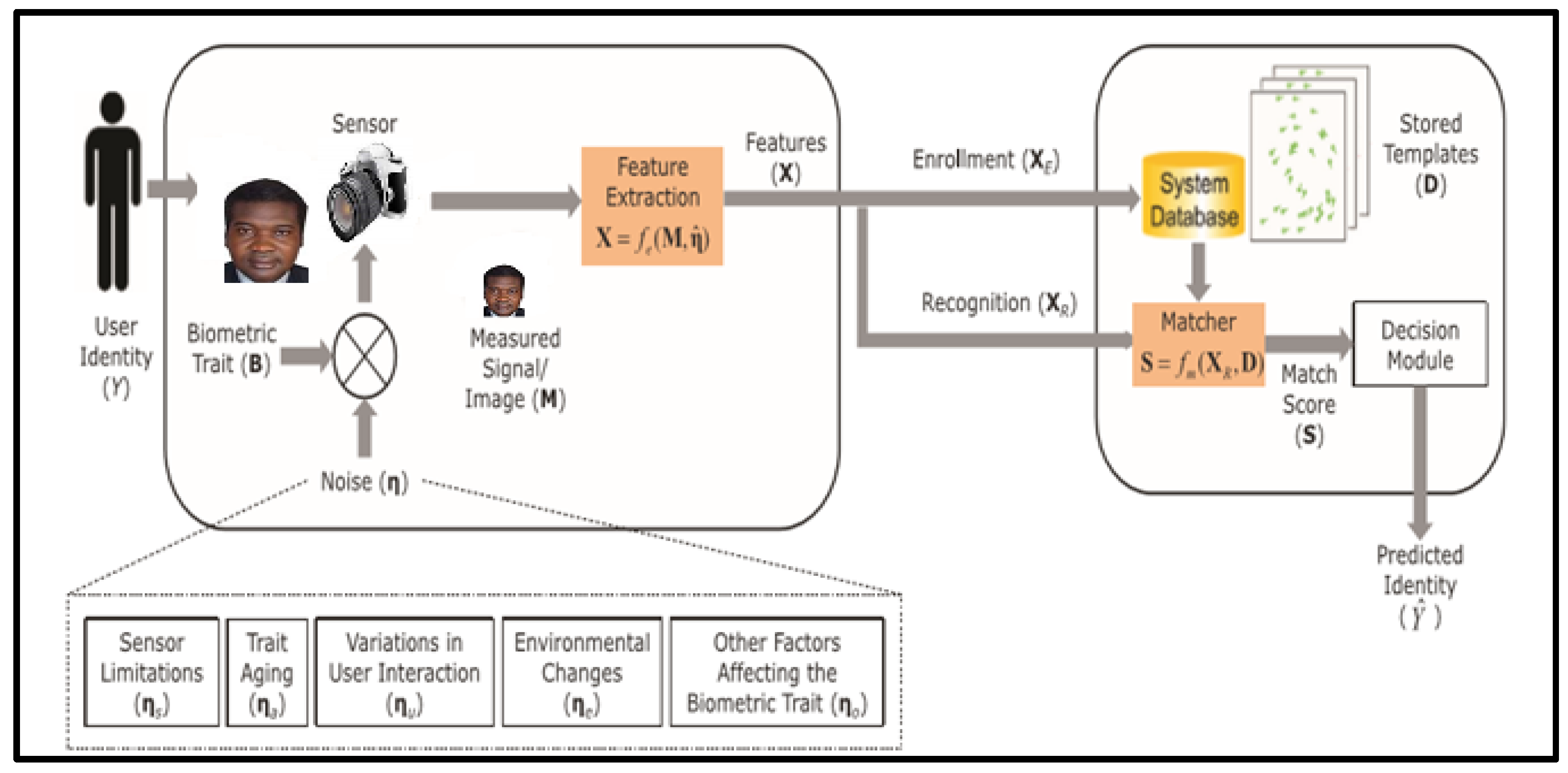
Trait aging in face recognition systems is a challenge that has been met with a low success rate through numerous hypotheses, models, and suggestions [6]. A complex mechanism known as trait-ageing variant characteristic of the face has been identified in a number of fields, including human perceptual abilities, digital image processing, pattern recognition, biology, and, more recently, biometrics. The contour and texture of the face are changed by trait ageing, which varies according to the age and time interval. From infancy to maturity, the impacts are primarily seen as a geometric shift on the face. While ageing modifies the texture of the face from adulthood to old age (e.g., wrinkles) [7]. Some of the extrinsic factors influencing face recognition systems are sensor restriction (distance from the camera), spatial precision, acquisition spectra (visible vs. infrared), the rate of frames (2D vs. 3D), and variations in user engagement (expression and position). In addition, lifestyle and environmental changes, such as occlusion, lighting, makeup, accessories, and backdrop scenarios, are further considerations. The face recognition system considers these factors as noises. The operation of a typical biometric system is depicted in Figure 1.

The age variant face recognition falls under the general category of face recognition and impacts security solutions including the deployment of human biometric devices, like surveillance cameras. The problem is complex because human participants' appearances in training or enrollment photographs can differ significantly from their appearances during the final recognition. The publicly available datasets for Ageing Invariant Face Recognition (AIFR) experimentation are very limited. The limitation cuts across the number of images in the dataset and race biases. The size of the publicly available datasets has made it challenging to apply convolutional neural networks in this domain without being over-fitted [8].

Convolutional Neural Networks (CNNs) have demonstrated exceptional performance in several domains in recent years, including image classification, object identification, and face recognition. CNN uses many types of convolutional and pooling layers to extract characteristics from images. CNNs can resolve numerous tasks involving visual recognition because of their strong feature extraction and learning capabilities. Some of the drawbacks of these CNN architectures are prohibitive computational cost, the need for substantial training data and so on [9].

Figure 1. Operation of a typical biometric system [10].

Figure 1. Operation of a typical biometric system [10].

Some scholars have suggested useful remedies, like data augmentation, regularization, dropout, batch normalization, and different activation functions, to lessen these disadvantages. CNN architectures have been expanding at a very quick pace since LeNet-5 [11], followed by AlexNet [12] and to GoogLeNet [13], VGGNet [14], ResNet [15], Inception network [16], Inception- ResNet [17] and so on. Responses from both academics and practitioners emphasize the several advantages of CNNs. For this research work, pre-trained; inception-ResNet-v3, ResNet-18, and Inception-v3 architectures are adopted in carrying out these experiments.

Automated face recognition is fast becoming a global trend as developing countries are already adopting it alongside developed countries. Such applications include security purposes such as surveillance cameras in the airport, border control, elections, and access control (for example, enabling individuals to lock and unlock devices) [18]. Nonetheless, most biometrics researchers and practitioners have not properly considered the genetic influences on face recognition systems, such as ageing of facial traits [19].

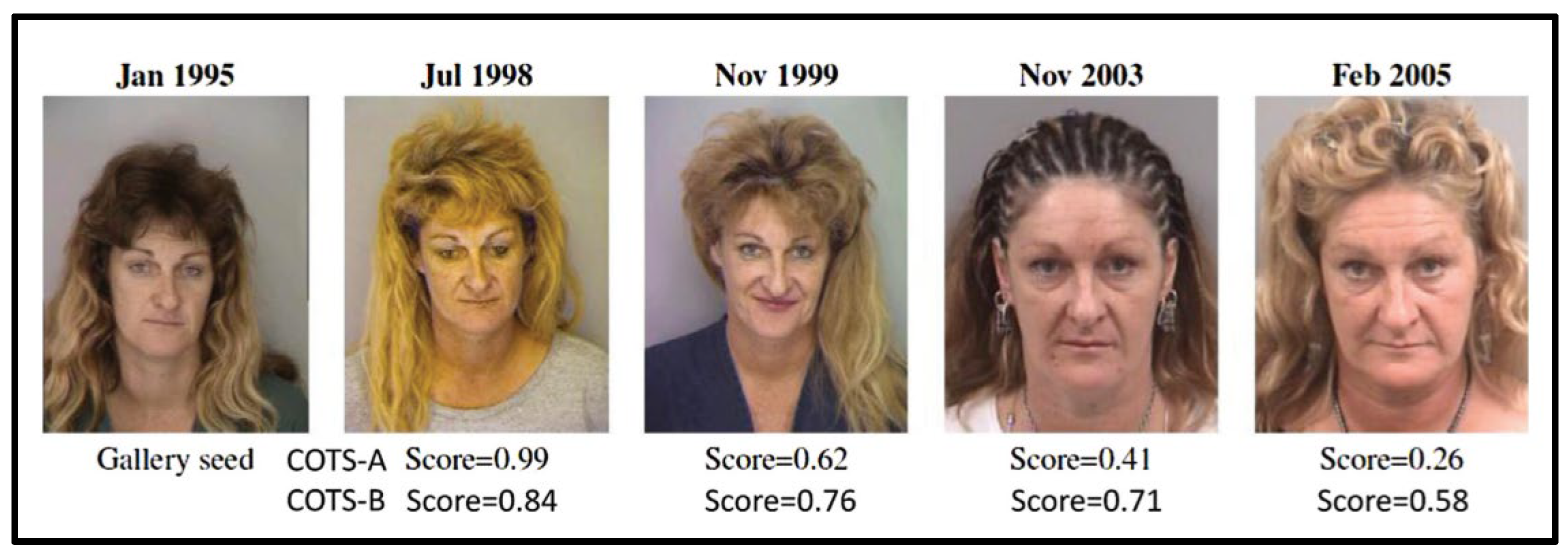
Figure 2 shows the face images of an individual captured over ten years. The Pinellas County Sheriff's Office (PCSO) submitted a mugshot record from which the subject photographs were taken. Think of the first image on the left as the analysis image, and the remaining images as the gallery seed. It is easy to see that when the interval between the gallery and probe photos lengthened, the match scores produced by two Commercial-Off-The-Shelf (COTS) face matches (designated as A and B) considerably decreased. Observe that the COTS-B matcher appears to be more resilient to ageing than the COTS-A matcher, indicating that COTS-B's face template compensates for face trait aging more well than COTS-A's [5]. A surveillance recognition camera will not be able to classify this subject correctly within these few years, depending on the device's given threshold.

The creation of a system for face recognition that is age-invariant if fully exploited by researchers stands to solve the problem of re-enrolment of individuals who utilize these systems. A robust data augmentation algorithm would improve face recognition, thus tackling the challenge of face variations due to trait ageing [18]. A model built using the robust augmentation algorithm would address the problem of trait ageing.

The publicly available dataset for Ageing Invariant Face Recognition (AIFR) experimentations is limited [19]. The limitation cuts across limited numbers of images in the dataset and race biases. The limited size of the publicly and globally accepted available AIFR datasets has made it difficult for the application of CNN in the domain without being over-fitted [20].

Figure 2. A facial recognition system's accuracy declining as a result of phenotypic ageing [5].

Figure 2. A facial recognition system's accuracy declining as a result of phenotypic ageing [5].

In this research work, the aforementioned challenges are addressed by developing a robust data augmentation algorithm for one of the most widely used AIFR datasets (Face and Gesture Recognition Network Ageing Database [FG-NET-AD]). Also, to make the research relevant to Africans, some African subjects are added to the FG-NET dataset to create a heterogeneous AIFR dataset.

This research uses data augmentation techniques to build enhanced models for age-invariant face recognition systems. The objectives of this research were to: acquire human face images of African subjects representative of their age progression; curate a heterogeneous human face image dataset of African and Caucasian subjects suitable for age-invariant face recognition; extend the developed heterogeneous dataset using appropriate data augmentation techniques; develop a robust age invariant face recognition models using pre-trained convolutional neural networks; and evaluate the models’ performance employing biometric classification standard metrics.

In summarising related works, the authors employed a number of methods to increase age-invariant facial recognition accuracy using the FG-NET dataset and different experimental setups and procedures. The following were not put into consideration by the earlier works done:

• The FG-NET dataset is a mono-race age variant face recognition dataset that does not cover the black race subjects, and Africans cannot use such models.
• The FG-NET dataset is an imbalanced dataset (all the classes do not have equal numbers of image samples). Therefore, accuracy as an evaluation metric will not reflect the actual performance of the AIFR model that is built on FG-NET [22,23].

This research work contributed the following to the body of knowledge:

• Using the developed heterogeneous dataset and the modified Face and Gesture Recognition Network Ageing Database (FG-NET AD), a pre-trained convolutional neural network designed for the generic image recognition problem was adapted to create robust novel models capable of handling age-invariant face recognition.
• The capacity to employ various forms of noise augmentation to raise the precision of the AIFR system, as opposed to the custom of removing noise during the pre-processing stage to raise the output accuracy, is another innovative aspect of this research. This research also breaks from the conventional approach of eliminating noise during the pre-processing stage to increase output accuracy by utilizing various forms of noise augmentation.

2. Materials and Methods

This section describes the development of a heterogeneous age invariant face recognition dataset and three types of experimental dataset setup utilized in section. Figure 3 is the architecture used to produce Model-1 to Model-9 using the developed heterogeneous dataset and three state-of-the-art CNNs networks.

Figure 3. The Architecture used in producing Models based on the Heterogeneous.

Figure 3. The Architecture used in producing Models based on the Heterogeneous.

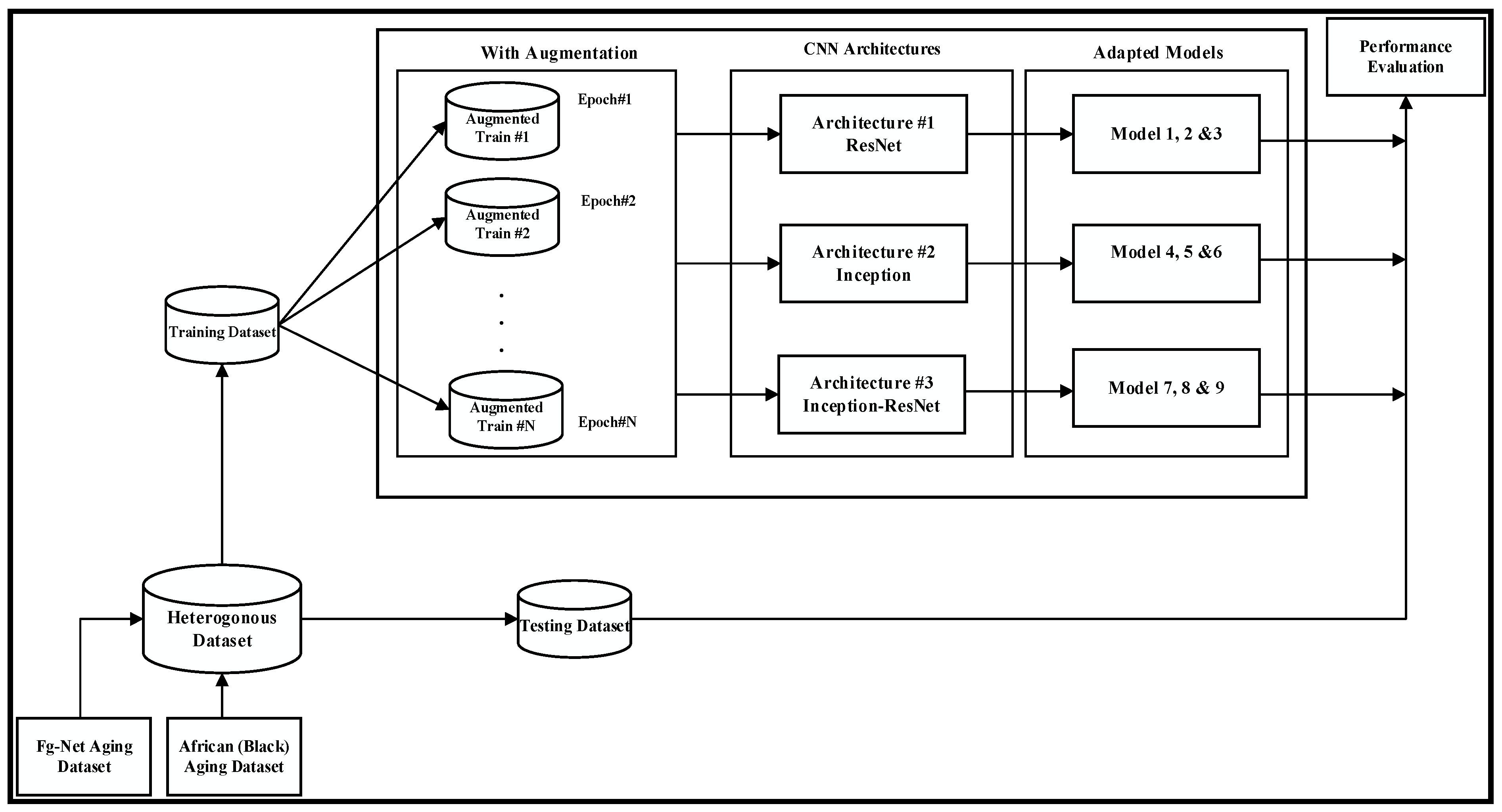
Table 1 shows the dataset types and pre-trained CNN architecture used to develop each model. For example, model-2 is the product of dataset-1 trained with pre-trained Resnet-18, while model-10 is the output of dataset-3 trained with pre-trained Inception-Resnet-v2.

2.1.1. Development of a Heterogeneous Age Invariant Face Recognition Dataset

The original dataset (FG-NET) is updated with 11 additional subjects to check the operation of the suggested technique on a different race of humans, ‘Africans’, which is not present in the original dataset. Now, the total sum of subjects in the dataset is 93. The 11 additional African subjects consist of 143 images, which are between the age ranges of 0 to 46. Approximately 7–24 facial photos of the same subject at various ages are also included. African respondent samples are displayed in Figure 4.

Large data sets are needed to train deep-learning models. Given that the FG-NET Dataset is a modest dataset for deep learning use, it comprises around 6–18 face photographs of a single participant at various ages. Consequently, picture noise addition and image geometric transformation are used to supplement the datasets. There is a discussion of three distinct experimental data setups where each image is read one at a time from the dataset and given the following operations for every version of the dataset:

Dataset-1 (All facial images without noises and geometric augmentations)

• To ensure that every image in the dataset has the same amount of channels, transform it to RGB if the image is grayscale.
• Use the Sliding Windows Face Detector to find and clip the subject's face to eliminate background distractions and enable the deep learning model to extract more detailed and pertinent characteristics.

Dataset-2 (All facial images with noises augmentation only)

• Ensure that every image in the dataset has the same number of channels by converting any grayscale images to RGB images.
• Locate and crop the subject's face using the sliding windows face detector to reduce background noise and make it easier for the deep learning algorithm to acquire relevant and in-depth information.
• Create three distinct iterations of the cropped image by including the various noise types mentioned below:

■

No noise (original cropped image with the only face)

■

Gaussian Noise

■

Salt and Pepper Noise

Adding noise will increase the dataset's image count without overfitting the network, and improved feature representation is extracted.

Dataset-3 (All facial images with noises and geometric augmentations)

• To ensure that every image in the dataset has the same amount of channels, if the image is grayscale, convert it to RGB.
• To enable the deep learning algorithm to acquire richer and pertinent characteristics, recognize and crop the subject's face using the sliding Windows Face Detector to eliminate background noise.
• Create three distinct iterations of the cropped image by including the various noise types mentioned below:

■

No noise (original cropped image with the only face)

■

Gaussian Noise

■

Salt and Pepper Noise

d.

Further, augment the images using random geometric transformations using an image augmenter with the outlined properties:

A leftward and rightward reflection

■

A leftward and rightward reflection

■

A leftward and rightward reflection

■

Reflection in the direction of top to bottom

■

An angle of rotation between 0 and 360°

■

Scaling using a factor between 0.5 and 2

■

Translation horizontally between -10 and 10 pixels

■

Translation from -10 to 10 pixels vertically

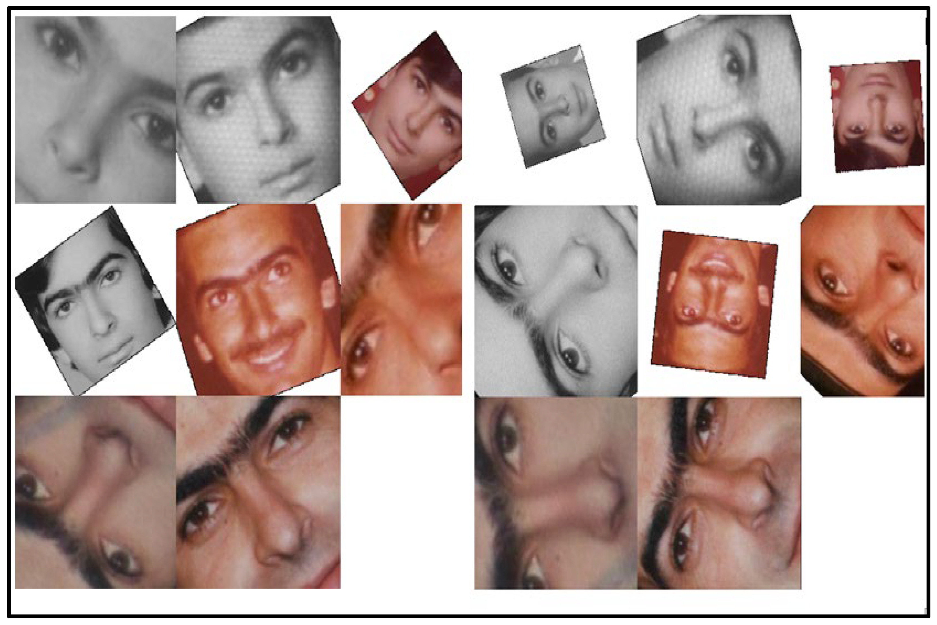
The augmentedImageDatastore in MATLAB is utilized to erratically alter the training picture sets for every epoch, utilizing marginally distinct data sets for every epoch. The converted images are not kept in memory at each epoch, nor is the actual number of training photos (online). Therefore, there isn't a rise in the quantity of images in the directory, which saves memory and time. In contrast, Figure 5 and Figure 6 show the facial image samples of a subject from the original FG-NET dataset and subject with different ages from the additional African subject added to the dataset. Figure 7 shows samples of noisy facial images of a subject, while Figure 8 shows samples of the random geometric transformations applied to facial images of a subject for Reflection, Rotation (0~360°), Scale (0.5~2), Horizontal Translation (-10 ~ 10px), Vertical Translation (-10 ~ 10px).

Figure 5. Facial images of a subject from original FG-NET Dataset.

Figure 5. Facial images of a subject from original FG-NET Dataset.

Figure 6. Facial images of a subject from the 11 additional African subjects added to the Dataset.

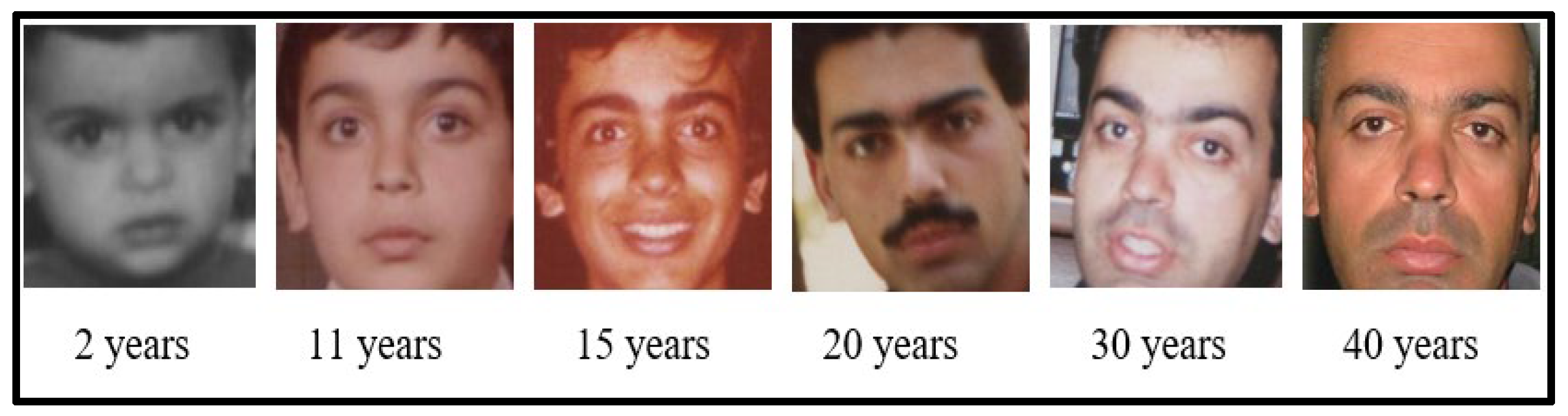
Figure 6. Facial images of a subject from the 11 additional African subjects added to the Dataset.

Figure 7. Samples of Noisy facial images of a subject.

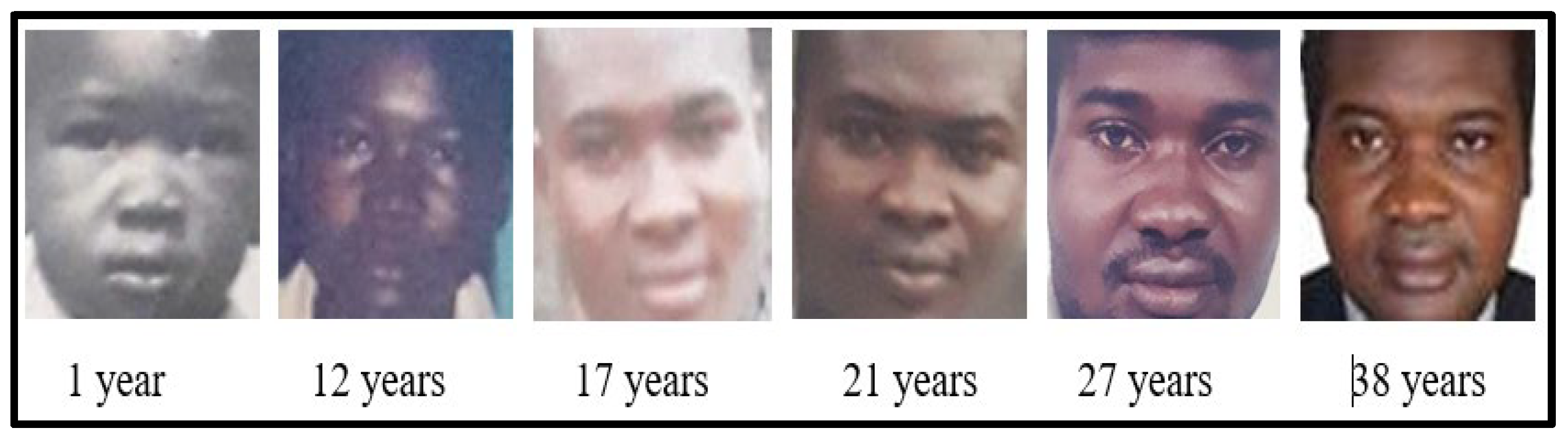
Figure 7. Samples of Noisy facial images of a subject.

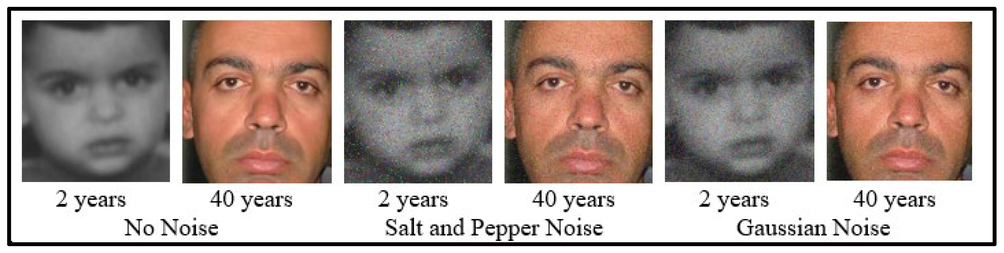
Figure 8. Random geometric transformations applied to facial images of a subject for Reflection, Rotation (0~360°), Scale (0.5~2), Horizontal Translation (-10 ~ 10px), Vertical Translation (-10 ~ 10px).

Figure 8. Random geometric transformations applied to facial images of a subject for Reflection, Rotation (0~360°), Scale (0.5~2), Horizontal Translation (-10 ~ 10px), Vertical Translation (-10 ~ 10px).

3.1.1. Training and Testing the Adapted CNN Models

Three pre-trained CNN models are trained via transfer learning on each dataset for facial recognition. Table 2 displays the details of three CNN models.

The training process is repeated for each adapted CNN model and each dataset. The steps involved are outlined in detail below:

• Split the dataset into a training set (70% images) and a validation set (30% images).
• All train and test sets photos should be resized to fit the CNN model's input size.
• As indicated in Table 3, provide training preferences and hyper-parameters for transfer learning.
• On the train set, train the previously trained network.
• Utilizing the validation set, assess the trained network.
• The network's performance should be assessed based on the accuracy and confusion matrix.

2.1.1. Platform Specifications

MATLAB R2018b was used to carry out the experimental set-up two on a computer system with 16GB RAM, Intel 2.3 GHz/64-bit quad-core processor. NVIDIA GPU with CUDA, 12GB memory and compute resources of 3.5 was utilized for training the CNN architectures in producing the models.

2.1.1. Methods Used for Models Evaluation and Validation

The measure employed to assess Model-1 to Model-9 performance (Experimental setup two: section two) is the derivations from the confusion matrix. Theses derivations include accuracy, positive predictive values and F-measured. This research work utilised heterogeneous dataset and as such appropriate to compare the models among themselves.

2.1. Terminology and Derivation from a Confusion Matrix

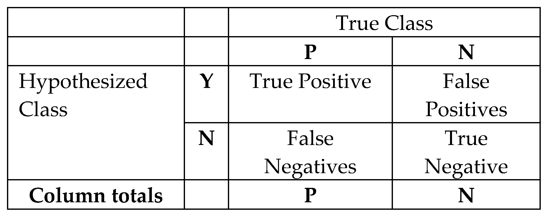
The terminology used in the confusion matrix are as presented in Figure 9 and defined as follows:

Condition Positive (P): The sum of real positive cases in the dataset (equivalent to True Positive plus False Negative)

Condition Negative (N): The number of actual negative occurrences in the dataset (equivalent to False Positive plus True Negative)

True Positive (TP): Equivalent with successfully classified. These are cases in which the model predicted yes (recognised), and they are correct.

True Negative (TN): Corresponding with correct rejection, that is the model predicted no, and the prediction is correct.

False Positive (FP): Corresponding with a false alarm, Type I error. The model predicted yes (recognised), but are incorrect.

False Negative (FN): Equivalent with unsuccessfully classified, Type II error. The model predicted no (not recognised), but they actually the correct image.

Figure 9. Confusion matrix.

Figure 9. Confusion matrix.

Some of the derivations from a Confusion Matrix are as shown in equations 1 to 7.

• Sensitivity, recall, hit rate, or True Positive Rate (TPR)

$$TPR={\displaystyle \frac{TP}{P}}={\displaystyle \frac{TP}{TP+FN}}$$

(1)

b.

Specificity, selectivity or True Negative Rate (TNR)

$$TNR={\displaystyle \frac{TN}{N}}={\displaystyle \frac{TN}{TN+FP}}=1-FPR$$

c.

Precision or Positive Predictive Value (PPV)

$$PPV={\displaystyle \frac{TP}{TP+FP}}=1-FDR$$

(3)

d.

Negative Predictive Value (NPV)

$$NPV={\displaystyle \frac{TN}{FN+TN}}=1-FOR$$

(4)

e.

Miss rate or False Negative Rate (FNR)

$$FNR={\displaystyle \frac{FN}{P}}={\displaystyle \frac{FN}{TP+FN}}=1-TPR$$

(5)

f.

Accuracy (ACC)

$$ACC={\displaystyle \frac{TP+TN}{P+N}}={\displaystyle \frac{TP+TN}{TP+TN+FP+FN}}$$

(6)

g.

F-Measure (F1 score) is the harmonic mean of precision and sensitivity

$$F-Measure={\displaystyle \frac{2\ast PPV\ast TPR}{PPV+TPR}}={\displaystyle \frac{2TP}{2TP+FP+FN}}$$

(7)

2.1.1. Evaluating Multi-Class Classification Performance from Confusion Matrix

The confusion matrixes obtained from the experimentation in this research work consist of 93 by 93 (this is 93 rows and 93 columns). The genuine concentration of the true positive is displayed by the diagonal running from top left to bottom right (the images that are correctly classified). While images classify as false positive are any values on each row other than the once along the row that is not in the diagonal matrix. Similarly, any other values on the columns of the confusion matrix other than the diagonal matrix are term false negative. The true negative is the summation of all other values other than the row, column or diagonal of the class under consideration. An illustrative example of the confusion matrix for a multi-class classification problem with the classes (A, B, C, and D); which is 4 by 4 is as shown in Table 4.

As illustrated in Table 4 ${TP}_A,{TP}_B$, ${TP}_C$ and ${TP}_D$ are the numbers of the true positive sample of class A, class B, class C and class D., For example, using class B as an illustration, this means ${TP}_B$ is correctly classified. While the value of samples classes A, C and D are, misclassify in the class B Column. $E_{BA},E_{BC},and{E}_{BD}$ are the samples from classes A, C and D, which are misclassified as class B, these are the incorrectly classified samples. Therefore, the misclassified values in all other columns other than the correct class are regarded as false negative; that is the false negative of A, B, C, and D classes are denoted as ${FN}_A,{FN}_B,{FN}_C{andFN}_D$ respectively. Equation 8 to Equation 11 shown that the mathematical expressions are extracts from Table 4.

$${FN}_A=E_{AB}+E_{AC}+E_{AD}$$

(8)

$${FN}_B=E_{BA}+E_{BC}+E_{BD}$$

(9)

$${FN}_C=E_{CA}+E_{CB}+E_{CD }$$

(10)

$${FN}_D=E_{DA}+E_{DB}+E_{DC}$$

(11)

In summary, the false negative ( $\mathrm{F}\mathrm{N}x$ ) Any multiclass could be calculated by summating all the error class values in the correct class column. Where x is the class under consideration.

Similarly, for every anticipated class, the false positive is located on the row of the correct class. For instance, as illustrated in Table 4

the false positive of class B are $E_{BA},E_{CA}and{E}_{DA}$ . Equation 12 to Equation 15 show the mathematical expression for illustration.

$${FP}_A=E_{BA}+E_{CA}+E_{DA}$$

(12)

$${FP}_B=E_{AB}+E_{CB}+E_{DB}$$

(13)

$${FP}_C=E_{CA}+E_{BC}+E_{DC}$$

(14)

$${FP}_D=E_{AD}+E_{BD}+E_{CD}$$

(15)

Finally, the true negative of any class in multiclass classification is evaluated. True negative is the summation of true positive value, the class false positive value and the class false negative value minus the other values related to the under consideration on the confusion matrix. Equation 16 to Equation 19 shown the mathematical expressions of illustration regarding Table 4.

$${TN}_A=\left({TP}_A+{FP}_A+{FN}_A\right)-\left[\left({TP}_B+E_{CB}+E_{DB}\right)+\left(E_{BC}+{TP}_C+E_{DC}\right)+\left(E_{BD}+E_{CD}+{TP}_D\right)\right]$$

(16)

$${TN}_B=\left({TP}_B+{FP}_B+{FN}_A\right)-\left[\left({TP}_A+E_{CA}+E_{DA}\right)+\left(E_{AC}+{TP}_C+E_{DC}\right)+\left(E_{AD}+E_{CD}+{TP}_D\right)\right]$$

(17)

$${TN}_C=\left({TP}_C+{FP}_C+{FN}_C\right)-\left[\left({TP}_A+E_{BA}+E_{DA}\right)+\left(E_{AB}+{TP}_B+E_{DB}\right)+\left(E_{AD}+E_{BD}+{TP}_D\right)\right]$$

(18)

$${TN}_D=\left({TP}_D+{FP}_D+{FN}_D\right)-\left[\left({TP}_A+E_{BA}+E_{CA}\right)+\left(E_{AB}+{TP}_B+E_{CB}\right)+\left(E_{AC}+E_{BC}+{TP}_C\right)\right]$$

(19)

In this research work, a multi-class of $93x93$ confusion matrix was the output result generated by the experimental performance evaluation as illustrated by Equation 20

$$\left[\begin{array}{c}{TP}_1 E_{\mathrm{2,1}}{E}_{\mathrm{3,1}} E_{\mathrm{4,1}}{E}_{\mathrm{5,1}}\dots \dots \dots \dots \dots \dots \dots \dots \dots \dots .E_{\mathrm{92,1}}{E}_{\mathrm{93,1}} \\ E_{\mathrm{1,2}}{TP}_2{E}_{\mathrm{3,2}}{E}_{\mathrm{4,2}} E_{\mathrm{5,2}}\dots \dots \dots \dots \dots \dots \dots \dots \dots \dots .E_{\mathrm{92,2}}{E}_{\mathrm{93,2}}\\ E_{\mathrm{1,3}} E_{\mathrm{2,3}} {TP}_3 E_{\mathrm{4,3}}{E}_{\mathrm{5,3}}\dots \dots \dots \dots \dots \dots \dots \dots \dots \dots .E_{\mathrm{92,3}}{E}_{\mathrm{93,3}}\\ \dots \dots \dots \dots \dots \dots \dots \dots \dots \dots \dots \dots .\dots \dots .\dots \dots \dots \dots \dots \dots \dots \dots \dots \dots \dots ..\\ \dots \dots \dots \dots \dots \dots \dots \dots \dots \dots \dots \dots \dots .\dots \dots .\dots \dots \dots \dots \dots \dots \dots \dots \dots \dots ..\\ \dots \dots \dots \dots \dots \dots \dots \dots \dots \dots \dots \dots \dots .\dots \dots \dots \dots \dots \dots \dots \dots \dots \dots \dots \dots \dots \\ E_{\mathrm{1,92}} E_{\mathrm{2,92}} E_{\mathrm{3,92}} E_{\mathrm{4,92}}{E}_{\mathrm{5,92}}\dots \dots \dots \dots \dots \dots \dots \dots .{TP}_{92} E_{\mathrm{93,92}}\\ E_{\mathrm{1,93}}{E}_{\mathrm{2,93}}{E}_{\mathrm{3,93}}{E}_{\mathrm{4,93}}{E}_{\mathrm{5,93}}\dots \dots \dots \dots \dots .\dots \dots \dots E_{\mathrm{92,93}}{TP}_{93}\end{array}\right]$$

(20)

Where the true positive is at the diagonal of the matrix from left-top to right bottom. These are true positive of class 1 to class 93 and represented as ${TP}_1,{TP}_2,{TP}_3,\dots \dots \dots {TP}_{92}and{TP}_{93}$

While the false-negative for class1 is the summation of the errors on the class1 column, as shown in Equation 21.

$${FN}_1=E_{\mathrm{1,2}}+E_{\mathrm{1,3}}+E_{\mathrm{1,4}}+E_{\mathrm{1,5}}+\dots \dots \dots \dots \dots \dots \dots .{+E}_{\mathrm{1,92}}+E_{\mathrm{1,93}}$$

(21)

Then the false positive for class 1 is the summation of the errors on class 1 row, as shown in Equation 22.

$${FP}_1=E_{\mathrm{2,1}}+E_{\mathrm{3,1}}+E_{\mathrm{4,1}}+E_{\mathrm{5,1}}+\dots \dots \dots \dots \dots \dots \dots \dots +E_{\mathrm{92,1}}+E_{\mathrm{93,1}}$$

(22)

Finally, the true negative for class1 is the summation of the true positive with the false positive and false negative of class1; subtracted from the summation of all others values on the rows, and columns (except for the values on the row and columns of class1). The true negative for class1 is as shown in Equation 23

$${\mathrm{T}\mathrm{N}}_1=\left({\mathrm{T}\mathrm{P}}_1+{\mathrm{F}\mathrm{P}}_1+{\mathrm{F}\mathrm{N}}_1\right)-\left(\begin{array}{c}\mathrm{summation} \mathrm{of} \mathrm{all} \mathrm{the} \mathrm{values} \mathrm{on} \mathrm{the} \\ \mathrm{confusion} \mathrm{matrix},\\ \mathrm{expect} \mathrm{row} 1 \mathrm{and} \mathrm{column} 1 \mathrm{associated}\\ \mathrm{with} \mathrm{class} 1\end{array}\right)$$

(23)

2.1.1. Micro-Average Method of a Multi-class Classification Problem

The interpretation of micro-averages and macro-averages in a multi-class classification issue varies because they compute somewhat differing effects. Each class's metric will be calculated independently by a macro-average, which will then take the average and treat all classes equally. To calculate the average metric, all class contributions will be combined into a micro-average at the same time. Because of the class unevenness in the multi-class categorization of this research experiment dataset, the micro-average is acceptable [23]. By adding together each set's unique false positives, true positives, false negatives, and true negatives for the system, you may apply the micro-average method to obtain statistics.

In a multi-class setting, micro-averaged FPR and TPR are in equation 23 and equation 24.

$$\mathrm{M}\mathrm{i}\mathrm{c}\mathrm{r}\mathrm{o}-\mathrm{a}\mathrm{v}\mathrm{e}\mathrm{r}\mathrm{a}\mathrm{g}\mathrm{e} \mathrm{o}\mathrm{f} \mathrm{F}\mathrm{P}\mathrm{R}={\displaystyle \frac{\sum _{\mathrm{c}=1}^{\mathrm{n}}{\mathrm{F}\mathrm{P}}_{\mathrm{c}}}{\sum _{\mathrm{c}=1}^{\mathrm{n}}{\mathrm{F}\mathrm{P}}_{\mathrm{c}}+\sum _{\mathrm{c}=1}^{\mathrm{n}}{\mathrm{T}\mathrm{N}}_{\mathrm{c}}}}$$

(24)

$$\mathrm{M}\mathrm{i}\mathrm{c}\mathrm{r}\mathrm{o}-\mathrm{a}\mathrm{v}\mathrm{e}\mathrm{r}\mathrm{a}\mathrm{g}\mathrm{e} \mathrm{o}\mathrm{f} \mathrm{T}\mathrm{P}\mathrm{R}={\displaystyle \frac{\sum _{\mathrm{c}=1}^{\mathrm{n}}{\mathrm{T}\mathrm{P}}_{\mathrm{c}}}{\sum _{\mathrm{c}=1}^{\mathrm{n}}{\mathrm{T}\mathrm{P}}_{\mathrm{c}}+\sum _{\mathrm{c}=1}^{\mathrm{n}}{\mathrm{F}\mathrm{N}}_{\mathrm{c}}}}$$

(25)

Where c is the position of class and n is the maximum number of class.

3. Results

This section is divided into subheadings. It concisely and precisely describes the experimental results, their interpretation, and the conclusions drawn.

3.1. Experimental Results

In this section, the experimental results are presented for model-1 to model-9. Adapted ResNet-18 architecture for dataset-1, dataset-2, and dataset-3 are used to simulate and develop Model-1, Model-2, and Model-3, respectively. In contrast, adapted Inception-v3 architecture for dataset-1, dataset-2, and dataset-3 are used to simulate and develop Model-4, Model-5, and Model-6, respectively. Finally adapted Inception-ResNet-v2 architecture for dataset-1, dataset-2, and dataset-3 are used to develop Model-7, Model-8, and Model-9, respectively.

3.1.1. Confusion Matrices of the Various CNNs Models

Figure 10 to Figure 18 displays the experimental outcomes of Model-1 to Model-9 in the form of confusion matrixes.

Figure 10. Confusion Matrix of Model-1 .

Figure 10. Confusion Matrix of Model-1 .

Figure 11. Confusion Matrix of Model-4.

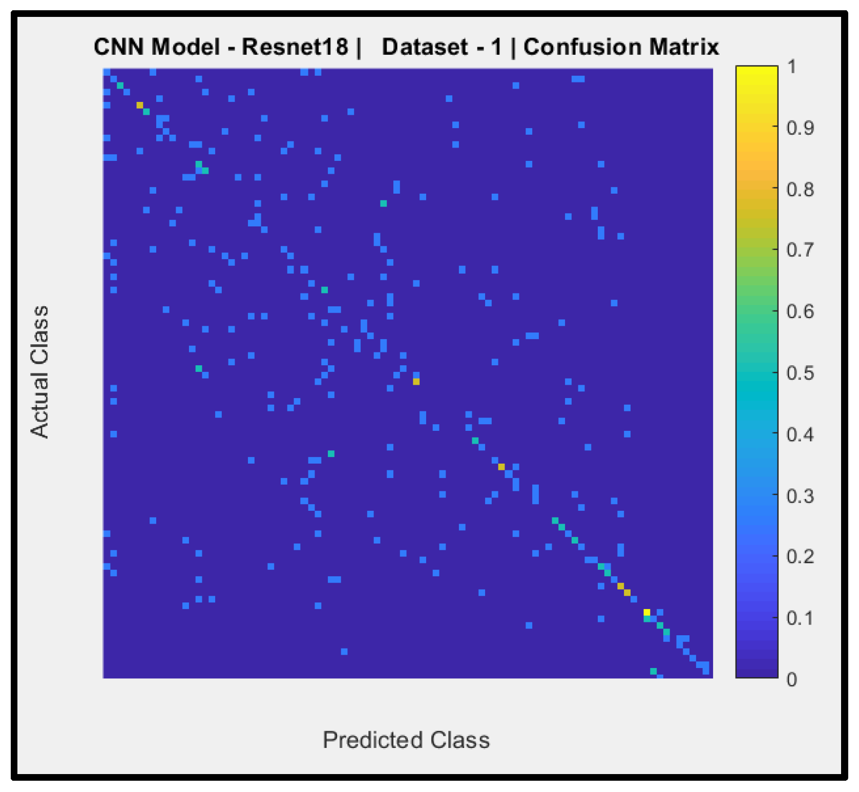
Figure 11. Confusion Matrix of Model-4.

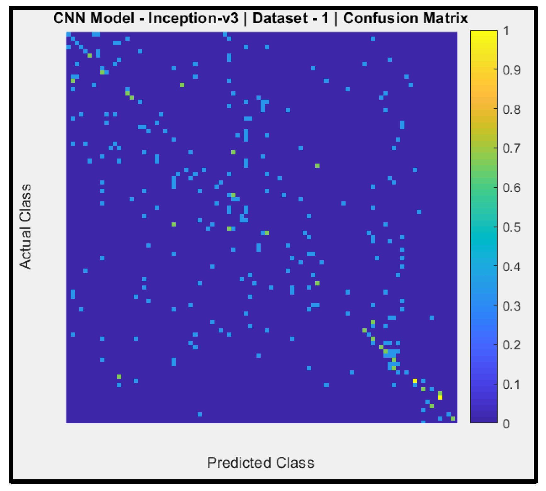
Figure 10 reveals a confusion matrix of the predictions of CNN Model-1 (pertained ResNet-18) with dataset-1. The y-axis denotes the actual AIFR images, and the x-axis is the predicted AIFR images. Model-1 mostly unable to predicts the correct AIFR images, with some random right classifications (six out of ninety-three).

Figure 11 shows a confusion matrix of the predictions of CNN Model-4 (pertained Inception-v3) with dataset-1. The y-axis signifies the actual AIFR images, and the x-axis is the predicted AIFR images. Model-4 mostly unable to predicts the correct AIFR images, with very few random right classifications (four out of ninety-three).

Figure 12. Confusion Matrix of Model-7.

Figure 12. Confusion Matrix of Model-7.

Figure 13. Confusion Matrix of Model-2.

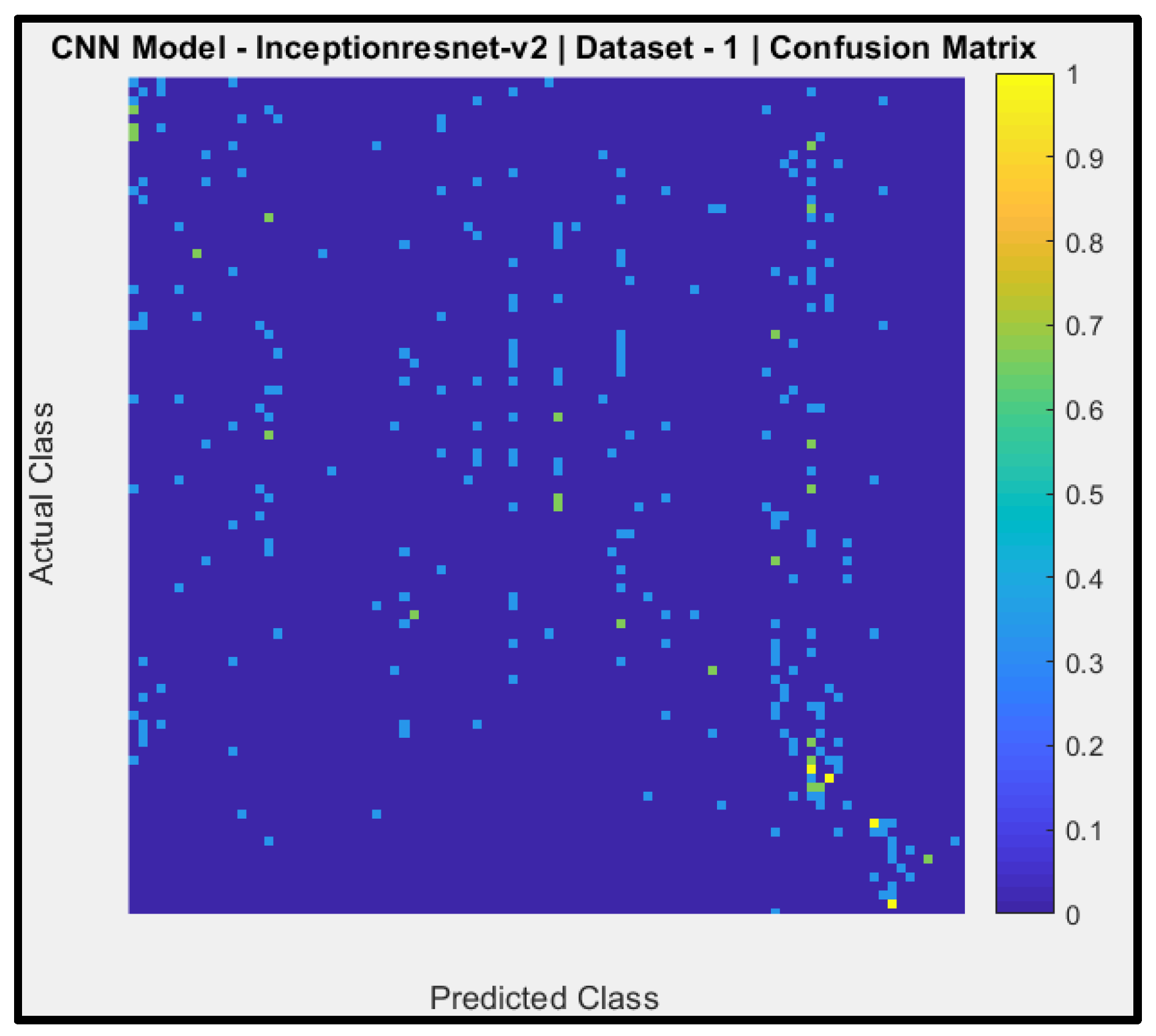
Figure 13. Confusion Matrix of Model-2.

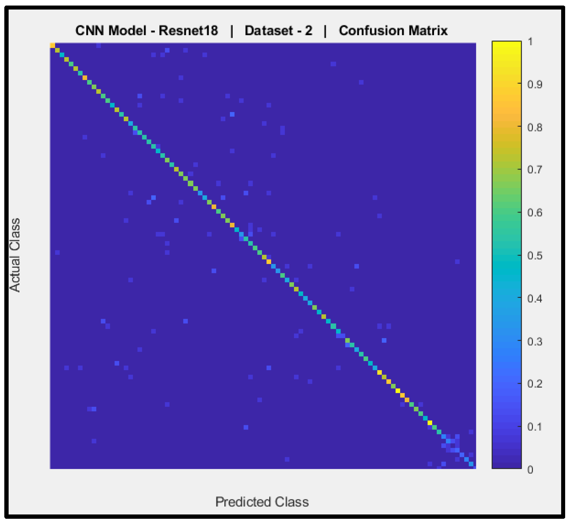
Figure 12 shows a confusion matrix of the predictions of CNN Model-7 (per-trained Inception-ResNet-v2) with dataset-1. The y-axis denotes the actual AIFR images, and the x-axis is the predicted AIFR images. Model-7 cannot predict the correct AIFR images, with no right classifications (zero out of ninety-three).

Figure 13 shows a confusion matrix of the predictions of CNN Model-2 (pre-trained ResNet-18) with dataset-2. The y-axis denotes the actual AIFR images, and the x-axis is the predicted AIFR images. Model-2 is mostly able to predict the correct AIFR images, with some random wrong classifications (ten out of ninety-three).

Figure 14. Confusion Result of Model-5.

Figure 14. Confusion Result of Model-5.

Figure 15. Confusion Matrix of Model-8.

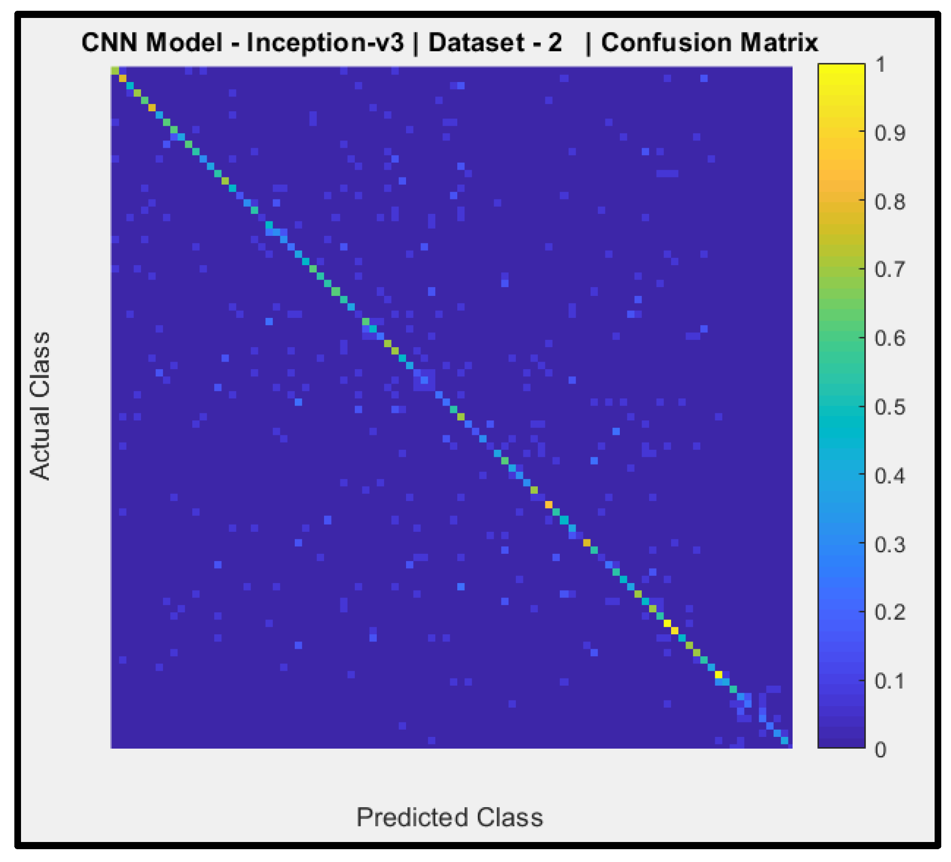
Figure 15. Confusion Matrix of Model-8.

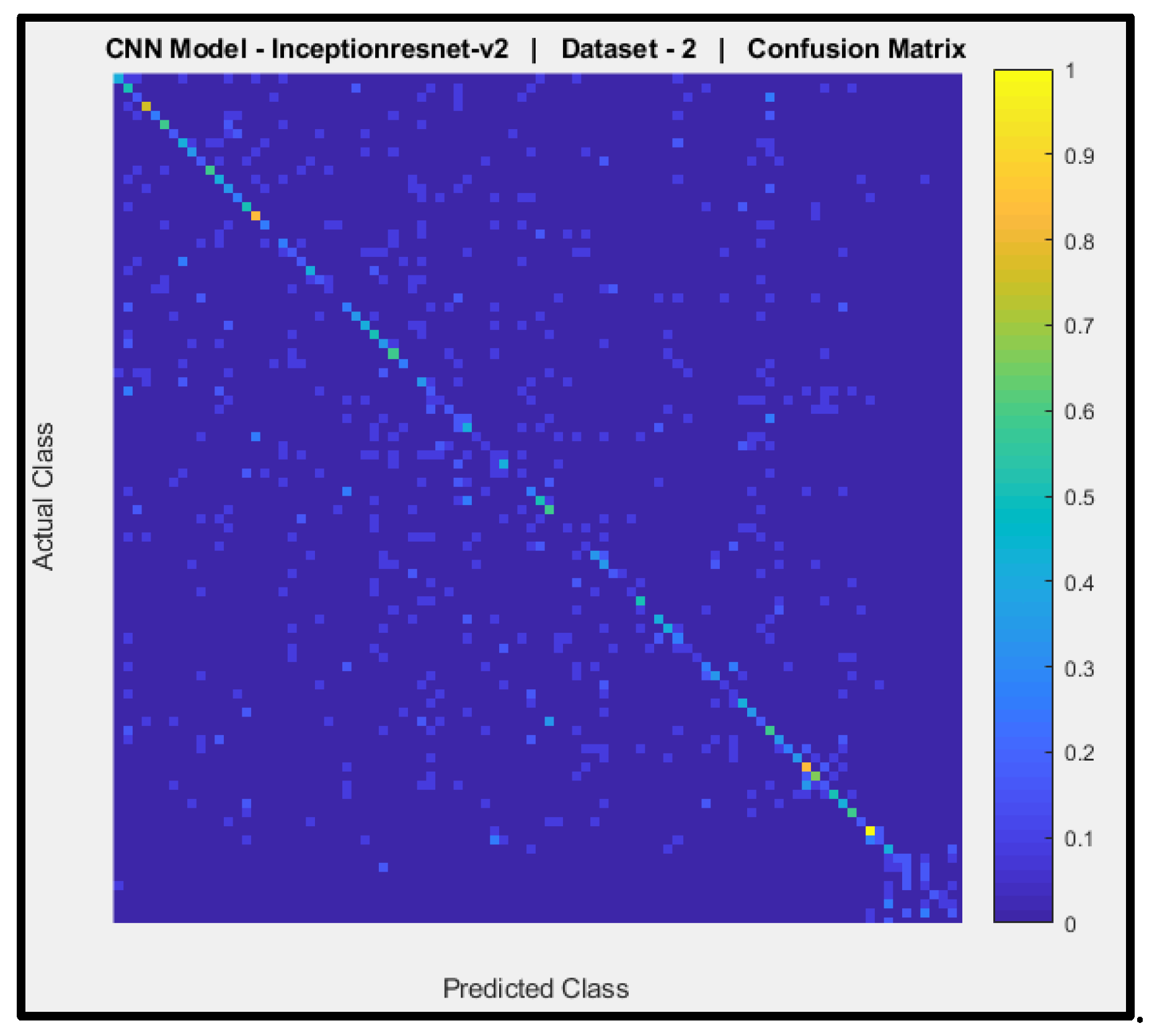
Figure 14 reveals a confusion matrix of the predictions of CNN Model-5 (pre-trained Inception-v3) with dataset-2. The y-axis signifies the actual AIFR images, and the x-axis is the predicted AIFR images. Model-5 can predict the correct AIFR images, with some random wrong classifications (thirty-nine out of ninety-three).

Figure 15 shows a confusion matrix of the predictions of CNN Model-8 (pre-trained Inception-ResNet-v2) with dataset-2. The y-axis signifies the actual AIFR images, and the x-axis is the predicted AIFR images. Model-8 cannot predict the correct AIFR images, with few random right classifications (nine out of ninety-three).

Figure 16. Confusion Matrix of Model-3.

Figure 16. Confusion Matrix of Model-3.

Figure 17. Confusion Matrix of Model-6.

Figure 17. Confusion Matrix of Model-6.

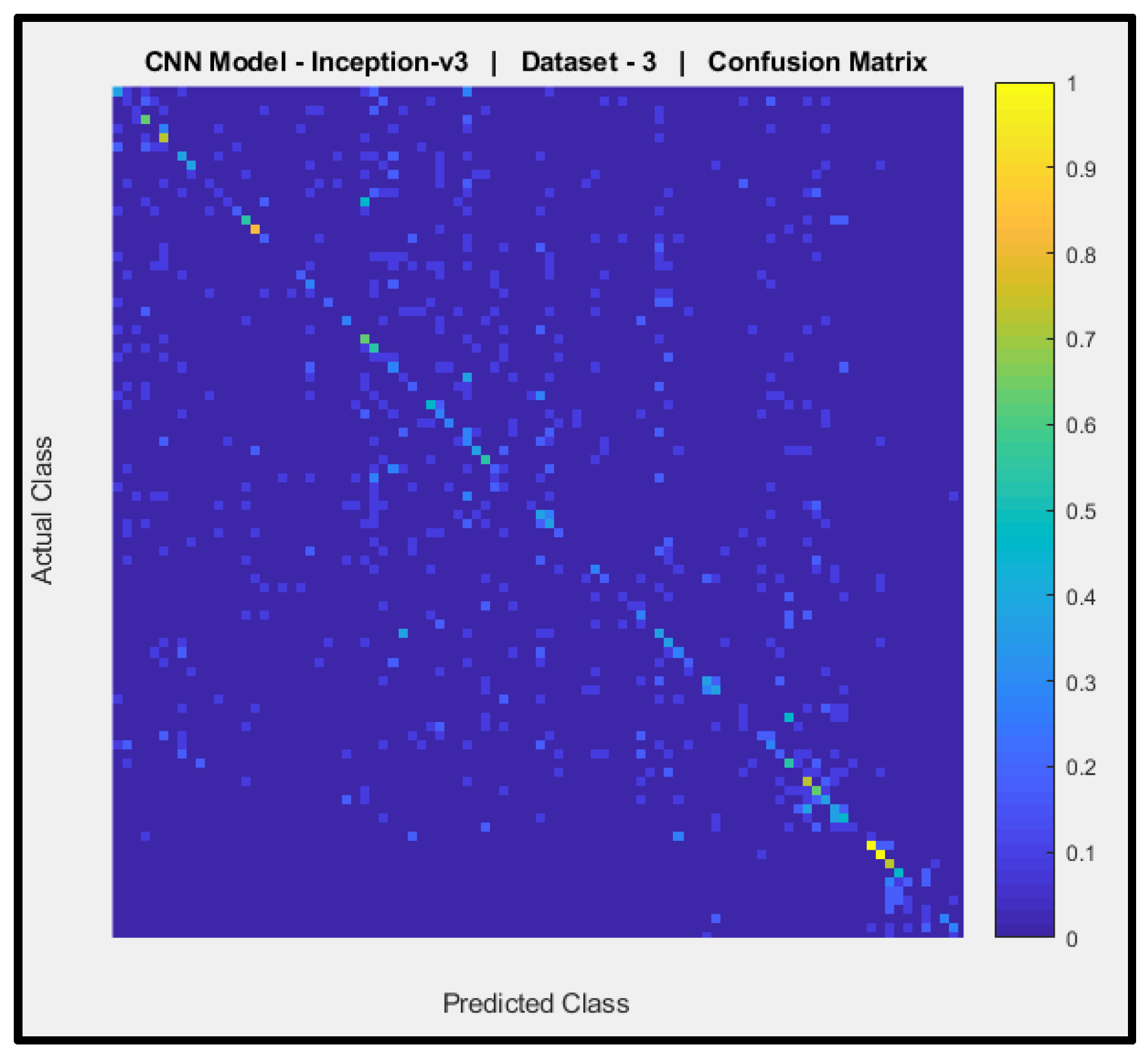
Figure 16 shows a confusion matrix of the predictions of CNN Model-3 (pre-trained ResNet-18) with dataset-3. The y-axis denotes the actual AIFR images, and the x-axis is the predicted AIFR images. Model-3 mostly cannot predict the correct AIFR images, with some random right classifications (nine out of ninety-three).

Figure 17 shows a confusion matrix of the predictions of CNN Model-6 (pre-trained Inception-v3) with dataset-3. The y-axis denotes the actual AIFR images, and the x-axis is the predicted AIFR images. Model-6 is mostly unable to predict the correct AIFR images, with few random right classifications (nine out of ninety-three).

Figure 18. Confusion Matrix of Model-9.

Figure 18. Confusion Matrix of Model-9.

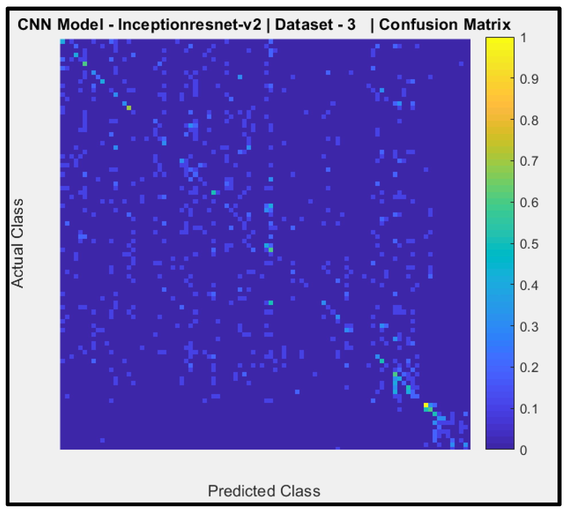
Figure 18 shows a confusion matrix of the predictions of CNN Model-9 (pre-trained Inception-ResNet-v2) with dataset-3. The y-axis denotes the actual AIFR images, and the x-axis is the predicted AIFR images. Model-9 is unable to predict the correct AIFR images, with very few random right classifications (two out of ninety-three).

Furthermore, a summary discussion of the experimental sections is highlighted as follows:

Rejected Models: In this experimental section, models are either accepted or rejected based on these three basic measured performance metrics. These metrics are accuracy, Predictive Positive Value, and F-measured.

In experimental section; model-1, model-3, model-4, model-6, model-7, model-8, and model-9, are completely rejected due to the following reasons:

Model-1, model-3, model-4, model-6, model-7, model-8, and model-9, attained the testing accuracies of 24.68%, 44.71%, 15.58%, 24.06%, 8.77%, 33.26% and 15.29% respectively. These results are below the average baseline. Thus, these models would highly misclassify the AIFR subjects.

Micro-average Predictive Positive Value (PPD), also called Precision for model-1, model-3, model-4, model-6, model-7, model-8, and model-9 are 23.25%, 21.57%, 13.98%, 21.58%, 13.93%, 28.9% and 13.58% respectively. Thus, these models could not predict the AIFR subjects correctly.

The value of the F-measure signifies the harmonic mean of precision and recall and stretches from zero to one, and high values of the F-measure indicate elevated classification performance. The F-measures mean of model-1, model-3, model-4, model-6, model-7, model-8, and model-9 are 0.24, 0.21, 0.14, 0.21, 0.048, 0.31 and 0.13 respectively. These F-measured results are below the average range of zero and one.

Marginally Accepted Model: In experimental set-up two, model-5 is marginally accepted due to the following reasons:

Model-5 attained an overall testing accuracy of 57.54%. This result is within the range of the average baseline. Thus, the model would marginally classify the AIFR subjects.

The model's micro-average Predictive Positive Value (PPD) is 55%. Thus, these models could predict the AIFR subjects a little bit correctly.

The F-measure of Model-5 is 0.55. This F-measured result is marginally above the average range of zero and one.

Clearly Accepted Model: In experimental section two, model-2 is clearly accepted due to the following reasons:

Model-2 attained an overall testing accuracy of 84.71%. This result is well above the baseline. Thus, the model would be able to classify the AIFR subjects significantly.

The model's micro-average Predictive Positive Value (PPD) is 77.73%. Thus, these models can predict the AIFR subjects correctly.

The F-measures of Model-2 is 0.85. This F-measured result is clearly above the average range of zero to one.

5. Conclusions

In this paper, the acquisition of human face images of African subjects’ representatives of their age progressions was collected after due permission and the signing of a legal agreement with the involved parties that the data will be used for research purposes only. The total number of images obtained is one-hundred and forty-three (143) from eleven (11) black individuals. Combining the acquired black ageing dataset and the FG-NET dataset formed a heterogeneous human face image dataset of African and Caucasian subjects suitable for age-invariant face recognition. Deep learning experiments need a large quantity of images in the dataset in order to avoid overfitting. The developed heterogeneous AIFR dataset is enlarged using both the noise injection and geometric transformation augmentation techniques. Subsequently, the pre-trained CNNs (ResNet, Inception, and Inception-ResNet) are adapted and trained with augmented heterogeneous AIFR datasets and models developed. The various developed models are validated with each of the appropriate testing data separately for this purpose, and the performances are evaluated.

The overall interest of this research work is to develop enhanced models for age-invariant face recognition using data augmentation techniques. The conclusions indicate that not all image data augmentation methods created using a convolutional neural network already trained for AIFR models are beneficial. This research clearly illustrates that noise injection image augmentation on AIFR models with pre-trained CNNs improves the performance of the systems. While geometric transformation image augmentation (such as reflection, rotation, scaling, and translation) on AIFR models with three pre-trained CNNs have minor (or insignificant) improvement on the system.

The relevance of this research work is that embedding the best performed (model-2) into surveillance cameras would help detect wanted persons via the facial traits of such individuals, even with wide age variation (for serval years). Furthermore, these embedded devices can also be deployed in access control, insurance, and renewals of national identification cards, international passports, driver’s licenses, etc. Renewing federal forms of identification becomes easier as applicants can upload their passport (face ID), and the system can identify the same person despite the age variations. This research addresses the intra-class facial variant of the same subject due to the ageing effect. Governments and industries are encouraged to invest in the integration and deployment of this model.

References

- K. Okokpujie, E. Noma-osaghae, S. John, K. Grace, and I. Okokpujie, “A Face Recognition Attendance System with GSM Notification,” in 2017 IEEE 3rd International Conference on Electro-Technology for National Development (NIGERCON) A, 2017, pp. 239–244. [CrossRef]
- H. El Khiyari and H. Wechsler, “Face Verification Subject to Varying ( Age, Ethnicity, and Gender ) Demographics Using Deep Learning,” J. Biom. Biostat., vol. 7, no. 4, 2016. [CrossRef]
- H. El Khiyari and H. Wechsler, “Age Invariant Face Recognition Using Convolutional Neural Networks and Set Distances,” J. Inf. Secur., vol. 8, pp. 174–185, 2017. [CrossRef]
- K. Okokpujie, S. John, C. Ndujiuba, J. Badejo, and E. Noma-Osaghae, “An improved age invariant face recognition using data augmentation,” Bull. Electr. Eng. Informatics, 10(1)., vol. 10, no. 1, pp. 1–15, 2021. [CrossRef]
- A. K. Jain, K. Nandakumar, and A. Ross, “50 years of biometric research: Accomplishments, challenges, and opportunities,” Pattern Recognit. Lett., vol. 79, no. January, pp. 80–105, 2016. [CrossRef]
- Dang, L. Minh, Kyungbok Min, Hanxiang Wang, Md Jalil Piran, Cheol Hee Lee, and Hyeonjoon Moon. "Sensor-based and vision-based human activity recognition: A comprehensive survey." Pattern Recognition 108 (2020): 107561. [CrossRef]
- R. Narayanan and C. Rama, “Modeling Age Progression in Young Faces Modeling Age Progression in Young Faces,” no. February, 2016. [CrossRef]
- Taherkhani, A., Cosma, G. and McGinnity, T.M., 2020. AdaBoost-CNN: An adaptive boosting algorithm for convolutional neural networks to classify multi-class imbalanced datasets using transfer learning. Neurocomputing, 404, pp.351-366. [CrossRef]
- Taye, Mohammad Mustafa. "Understanding of machine learning with deep learning: architectures, workflow, applications and future directions." Computers 12, no. 5 (2023): 91. [CrossRef]
- Okokpujie, K., Okokpujie, I.P., Abioye, F.A., Subair, R.E. and Vincent, A.A., 2024. Facial Anthropometry-Based Masked Face Recognition System. Ingenierie des Systemes d'Information, 29(3), p.809. [CrossRef]
- Y. Lecun, Y. Bengio, and G. Hinton, “Deep learning,” Nature, vol. 521, no. 7553, pp. 436–444, 2015. [CrossRef]
- A. Krizhevsky, I., Sutskever, and G. Hinton, “ImageNet Classification with Deep Convolutional Neural Networks,” Adv. Neural Inf. Process. Syst., pp. 1097–1105, 2012.
- C. Szegedy, V., Vanhoucke, J. Shlens, and Z. Wojna, “Rethinking the Inception Architecture for Computer Vision,” arXiv1512.00567v3 [cs.CV] 11 Dec 2015, pp. 1–10, 2015.
- S. Karen and Z. Andrew, “Very Deep Convolutional Networks For Large-Scale Image Recognition,” Publ. as a Conf. Pap. ICLR, vol. arXiv:1409, pp. 1–14, 2015. [CrossRef]
- H. Kaiming, X. Zhang, R. Shaoqing, and S. Jian, “Deep Residual Learning for Image Recognition,” in Proceedings of the IEEE conference on computer vision and pattern recognition, 2016, 2016, pp. 770–778.
- C. Szegedy, S. Reed, P. Sermanet, V. Vanhoucke, and A. Rabinovich, “Going deeper with convolutions,” arXiv1409.4842v1 17 Sep 2014, pp. 1–12, 2014.
- C. Szegedy, S. Ioffe, V. Vanhoucke, and A. Alemi, “The Impact of Residual Connections on Learning,” arXiv:1602.07261v2 [cs.CV] eprint, no. 8, pp. 1–12, 2016.
- C. Shorten and T. M. Khoshgoftaar, “A survey on Image Data Augmentation for Deep Learning,” J. Big Data, vol. 6, no. 60, pp. 1–48, 2019. [CrossRef]
- Okokpujie, K., Okokpujie, I.P., Subair, R.E., Simonyan, E.O. and Adenugba, V.A., 2023. Designing an adaptive Age-Invariant Face recognition system for enhanced security in smart urban environments. Ingenierie des Systemes d'Information, 28(4), p.815. [CrossRef]
- Qayyum, A., Ahmad, K., Ahsan, M.A., Al-Fuqaha, A. and Qadir, J., 2022. Collaborative federated learning for healthcare: Multi-modal covid-19 diagnosis at the edge. IEEE Open Journal of the Computer Society, 3, pp.172-184. [CrossRef]
- M. Johnson and T. M. Khoshgoftaar, “Survey on deep learning with class imbalance,” J. Big Data, vol. 6, no. 27, pp. 1–54, 2019. [CrossRef]
- A. Luque, A. Carrasco, A. Martín, and A. de las Heras, “The impact of class imbalance in classification performance metrics based on the binary confusion matrix,” Pattern Recognit., vol. 91, pp. 216–231, 2019. [CrossRef]
- R. Alejo, J. A. Antonio, R. M. Valdovinos, and J. H. Pacheco-Sánchez, “Assessments metrics for multi-class imbalance learning: A preliminary study,” Lect. Notes Comput. Sci. (including Subser. Lect. Notes Artif. Intell. Lect. Notes Bioinformatics), vol. 7914 LNCS, pp. 335–343, 2013, doi: 10.1007/978-3-642-38989-4_34.Author 1, A.; Author 2, B. Title of the chapter. In Book Title, 2nd ed.; Editor 1, A., Editor 2, B., Eds.; Publisher: Publisher Location, Country, 2007; Volume 3, pp. 154–196. [CrossRef]