
Submitted:
18 December 2024
Posted:
19 December 2024
You are already at the latest version
Abstract
Air pollution is a major issue with serious risks to human health and the environment. This study investigates air pollution concentrations in three cities with distinct characteristics: a city with high industrial activities, a city with high population and urbanization, and an agricultural city. The air pollution data was collected using the Sentinel-5P satellite and Google Earth Engine to apply descriptive analysis and comparison of two years, 2022 and 2023. The cities in Saudi Arabia were Al Riyadh (high population), Al Jubail (industrial), and Najran (agricultural). The selected pollutants were SO₂, NO₂, CO, O₃, and HCHO. In addition, the study investigates the variations observed in all the pollutants during the months of the year, the correlations between the pollutants, and the correlation between NO₂ and the meteorological data. Based on the findings, Al Jubail has the highest level of all the pollutants during the two years, except for NO₂, which has the highest level in Al Riyadh, which has witnessed notable urbanization development recently. Moreover, this study developed a forecasting model of the concentration of NO₂ based on the weather data and the previous values of NO₂ using Long Short-Term Memory (LSTM) and Time2Vec. The modeling proved that any model that is trained on data collected from a specific city is not suitable to predict the pollution level in another city and for another pollutant, as the three cities have different correlations to the pollutants and the weather data. The forecasting models are useful to enhance air quality monitoring and forecasting capabilities and support the implementation of proactive strategies to mitigate air pollution. The results of this study contribute to ongoing efforts to understand the dynamics of air pollution based on the city's characteristics and the period of the year.
Keywords:
Air Pollution
; Deep Learning
; Time-Series
; LSTM
; Prediction
; Time2Vector
1. Introduction
Air pollution is a global problem and a major societal concern because it affects health and the environment and causes significant damage over time. The emissions of huge amounts of gases into the air such as formaldehyde (HCHO), sulfur dioxide (SO₂), carbon monoxide (CO), nitrogen dioxide (NO₂), particulate matter (PM), and ozone (O₃) are the causes of air pollution according to the estimates of the World Health Organization (WHO) [1]. The most important sources of increasing concentration of these pollutants in the air are vehicle emissions, industry, fossil fuel combustion, deforestation, power plant smoke, etc. [2].
The WHO reports that approximately 4.2 million premature deaths worldwide are due to exposure to these pollutants [3]. These pollutants enter the respiratory tract and deposit in the lung area, causing serious diseases such as lung cancer, heart disease, and respiratory infections such as pneumonia [4]. Other factors that affect poor air quality include high temperature, humidity, population growth, and wind speed.
Air pollution is a major problem in Saudi cities as it is one of the largest energy-producing countries. The Saudi Green Initiative has contributed to promoting clean energy and reducing emissions in line with Vision 2030 for a better quality of life. Because air pollution is an important indicator of the quality of life in any city, this study aims to study the air pollution levels at three cities with different industrial, agricultural, and population density characteristics as these characteristics affect the air pollution level [5]. Moreover, this study aims to build a prediction model to accurately monitor the air pollution level based on the three cities’ data.
The three cities were Al Riyadh, Al Jubail, and Najran. Al Riyadh was chosen because it is densely populated in the center of Saudi Arabia and is the country’s capital and largest city. Rapid urban growth has brought challenges such as high levels of air pollution due to emissions from vehicles, industries, and construction projects, which are exacerbated by the city’s population density [6]. It has a hot desert climate with long, very hot summers, mild winters, and little yearly rainfall. Al Jubail is an industrial city on the eastern coast of Saudi Arabia along the Arabian Gulf. It is a major industrial center with petrochemical plants and manufacturing facilities [7]. The city’s economic growth is significant, but it faces challenges with air quality and pollution due to high industry emissions, which impact the environment and public health. It has a hot climate with high humidity in summer and mild in winter with limited rainfall throughout the year. Najran is an agricultural city in southwestern Saudi Arabia, with some industrial development [8]. This combination presents challenges and opportunities for pollution control. While agriculture results in lower pollution levels than industry, a balance between agriculture and industry is critical to maintaining air quality as Najran grows. It has a hot climate in summer and a mild winter with rainfall.
Future air pollution can be predicted using time series forecasting methods, as satellites provide essential information in many areas of global monitoring to understand the effects of climate change, forests, agricultural areas, and the development of large cities and how to deal with them [9]. The Sentinel-5 satellite is the first atmospheric composition mission of the Copernicus Air Pollution Control Program. It identifies gases such as O₃, HCHO, CO, NO₂, and SO₂ [10]. Satellite images from Sentinel-5 can effectively study the spatial distribution of pollutants due to their large global views of the Earth’s surface. As part of Sentinel-5, the TROPOMI (Tropospheric Monitoring Instrument) instrument was used. The sensor provides daily data on air pollution [11]. Many pollutants can be monitored and imaged using the TROPOMI sensor. Therefore, remote sensing is one of the most accurate methods for measuring air pollution, both temporally and spatially [12]. The pollutant dataset was collected via the Google Earth Engine (GEE) cloud computing platform using JavaScript programming in the Earth Engine code editor. GEE is an online computing platform that processes satellite imagery, geospatial data, and spatial data on a petabyte-scale [13]. It also provides access to software and algorithms for processing satellite data [14].
There are many regulations to control and address the level of air pollution and many efforts to enforce these regulations to improve air quality. Our study aims to contribute to these ongoing efforts through two main objectives:
-
Descriptive analysisBy investigating the air pollution trends of three cities with different environmental characteristics, we can comprehensively understand each city’s air pollution fluctuation throughout the year.
-
Predictive modelingDeveloping an accurate model to predict the future values of air pollution at a specific period can enhance the feasibility and applicability of monitoring policies at various places. This can provide warning systems for the areas at risk of elevated air pollution levels, which facilitates the task of monitoring teams.
The following sections constitute the bulk of the paper. The next section (section 2) provides a literature review and the background of the techniques used to build the proposed system. Then, section 3 explains our method of collecting and applying statistical analysis. Moreover, it presents our learning approach to develop the predictive model. After that, in section 4 we present and discuss the statistical results of the air pollutants in the three cities and the performance of the developed forecasting models. At the end of this paper, we present in section 5 the main conclusion of the research, limitations, and future directions for further research improvement.
2. Literature Review
2.1. Air Pollution Studies
Many studies have been conducted on air pollution in the cities of Saudi Arabia. Studies indicate that air pollution leads to human health problems such as respiratory diseases and heart diseases. They also discussed the sources of pollution and methods for assessing and improving air quality. The authors of [15] studied the relationship between pollution parameters and atmospheric factors including temperature and wind speed in the city of Al-Qurayyat in the Kingdom of Saudi Arabia, and satellite data was used instead of observed data from ground stations to detect the concentration rate of air pollutants including NO₂, SO₂, and CO. In addition, the region is exposed to frequent dust storms during the period of data collection, which are the main source of increasing levels of environmental pollutants [16] and are responsible for annual deaths that pose a risk to human health [17]. According to the World Health Organization (2018), Riyadh and Jubail are among the ten most polluted cities in the world, ranking fourth and fifth. They also studied the analysis of the correlation between air pollutants and atmospheric parameters, and the results showed that temperature and wind speed had a negative correlation. In contrast, relative humidity showed a positive correlation. The authors suggested that traffic and burning fossil fuels for electricity generation are the main causes of the high concentration of air pollutants. The authors believe that the results of this study are useful for decision-makers in knowing the levels of air pollutant concentrations in the study area. In [18], the authors discussed the air quality parameters in Makkah, Madinah, and Jeddah by analyzing the atmospheric parameters, temperature, relative humidity, and the relationship with air pollution from June to September 2019 and 2020. While air quality is generally affected during the Hajj season, during 2020, it showed a decrease in pollutant concentrations, and the COVID-19 pandemic had a positive impact due to the decrease in human activities [19]. In [20], the researchers studied the current and future air quality analysis in Riyadh using the Air Quality Index. Six major air pollutants were considered, namely NO₂, SO₂, PM, O₃, CO, and CO₂. The air quality in Al Riyadh was compared to the local, regional, and international levels. Factors such as seasons and working hours were considered. The main pollutants were identified as industrial emissions, fuel combustion, and wind-borne dust. Overall, the air quality components were below the required levels. Of all the pollutants studied, PM particles pose the greatest threat to human health in the city.
As mentioned previously, Al Riyadh and Al Jubail have exceptionally high levels of air pollution, which is expected due to the high population and urbanization of Al Riyadh and the high industrial activities in Al Jubail. In this study, we aimed to focus more on these two cities and compare them to the agricultural city, Najran, which has a low population density. Moreover, we wanted to avoid the periods of the COVID-19 pandemic as its effect has been studied extensively in many places in the world. Instead, we were more concerned about studying the effect of the normal activities of these three cities, all of which are undergoing continuous development to achieve the goals of Vision 2030. Hence, our study aimed to collect data from these three cities during the two years, 2022 and 2023, to facilitate the comparison of all the months of the two years, which allows studying the effect of different weather factors on three cities with different characteristics.
2.2. Remote Sensing for Air Quality Monitoring
A satellite is an object placed in outer space orbit to collect data faster than instruments on the ground [21]. It has a variety of uses for weather forecasting, GPS navigation, scientific research, broadcasting, and earth observation. Copernicus is the European Union’s Earth monitoring program, which includes the Sentinel satellite, which was before known as Global Monitoring Environment and Security (GMES). The program uses satellite data to provide a comprehensive set of terrestrial, atmospheric, and oceanographic parameters [22]. The Copernicus Program relies on its space segment of observational satellites, and measurements using airborne sensors. Copernicus’s data will be used to generate the time series of this research. The name “Sentinel” refers to the Copernicus satellite constellation. Sentinels and satellites belong to six families. Sentinel-1 maintains the continuity of the radar data gathered by Envisat and ERS. Sentinel-2 and 3 monitor oceans and land masses. Sentinel-6 ensures operational continuity for Jason altimetry missions, while Sentinel-4 and -5 are intended for meteorological and climate logical missions to ensure the availability of atmospheric data [22]. The concept of meteorology is the study of phenomena and the effects of the atmosphere on weather and climate. The analysis of the atmosphere focuses on weather forecasting processes. Weather phenomena are something meteorologists can monitor and interpret [23]. The power of deep learning can be used with satellite data to make suitable forecasts and provide experts with information about weather, climate, and the state of the planet. This allows them to prepare for storms, understand the impact of climate change, and develop plans to improve the use of natural resources and protect vulnerable populations.
2.3. Brief Background of Techniques
This section will provide insight into the background of relevant techniques used in this research which include deep learning models suitable for time series forecasting, what time series are, and an explanation of the Time2Vec algorithm.
2.3.1. LSTM
LSTM is a type of recurrent neural network (RNN) architecture. It can learn previous information and retain it in the long term. It solves one of the main problems of RNN, which is vanishing gradients. It helps with time series forecasting because it saves and remembers previous inputs for a long time [24]. LSTM has a string-like structure consisting of blocks of memory cells from which data flows through input, output, and forget gates. These gates are responsible for what is read, written, and stored in the cell, as shown in Figure 1, where X, C, and h symbolize the cell and its input and output values. The symbol t represents the value of the current time step and (t – 1) indicates the value of the past time step. The reference to tanh is the hyperbolic tangent; The function and σ represent the sigmoid function. The x and + operators are the multiplication and addition of elements, respectively.
2.3.2. Time Series
Time series is a term that refers to anything observed or tracked sequentially over time in the long or short term. It can be numbers, symbols, etc., and time can be continuous or discrete. Moreover, time series have different properties compared to other data types which are considered a challenge for analysis and modeling. To develop a model, the success of each implementation depends on the correct data design [25]. In addition, deep learning has been used for time series data, a common topic of interest in other fields such as financial forecasts, weather, solar energy, and electricity load [25].
2.3.3. Time2Vector
Time is crucial in applications with synchronous and asynchronous events. Time2Vec, a model-independent vector representation of time, is introduced to enhance performance in various architectures.
It can be combined with many deep learning models, such as convolutional neural networks and recurrent neural networks, to learn patterns in data and make predictions. Time2Vec can be used for forecasting, anomaly detection, and other applications related to time series analysis. It has been used in various fields such as stock prices, healthcare, energy, and sales [26]. Demonstrated through a set of models and problems that replacing the concept of time with the Time2Vec representation improves the performance of the final model. Instead of adding Time2Vec to other vector representations, the authors feed it into the model or some of its gates. Additionally, this representation provides the foundation for learning the appropriate time functions based on the data and does not require manual time functions. It is simple to incorporate time vector representations into existing deep-learning architectures. It has three properties: periodicity, simplicity, and remeasure at a fixed time [26]. For a given standard concept of time τ, the Time2Vec of τ, denoted t2v(τ), is a vector of size k + 1, as defined by the following equation:
F is a periodic activation sine function, ω and ϕ are learnable parameters, and where t2v(τ)[i] is the ith element of t2v(τ).
When 1 ≤ i ≤ k, ωi, and ϕi are the frequency and phase shifts of the sine function [26].
2.4. Deep Learning for Time Series Forecasting
Recently, with the development of deep learning methods and data analysis, prediction models based on data mining and deep learning techniques have become increasingly popular. Their prediction effectiveness judges the quality of models [27]. Deep learning algorithms have achieved outstanding performance in prediction and detection in various application fields, such as the financial market [28] and natural language processing [29,30].
Many researchers have used deep learning time series methods to address air pollution prediction problems, and one of the most common methods in deep learning techniques is LSTM. It is widely applied in many areas of time series prediction, especially in air pollution prediction. Previous research shows success in giving accurate predictions of air pollution parameters. Wang et el. [31] developed an air quality prediction model that combines multiple individual deep-learning models. The experiments conducted on the dataset collected from monitoring stations in Beijing showed that LSTM was more accurate than other deep learning models such as CNN. Moreover, some researchers also used the Time2Vec algorithm in different prediction areas such as stock prices, electricity consumption, and traffic flow [26]. It has proven its effectiveness and success with LSTM, so it was included in constructing the proposed model in this research. In [32], the authors demonstrated that combining the temporal feature extraction capabilities of LSTM with the spatial feature extraction capabilities of CNN and applying this combined model to diverse data types resulted in improved predictive performance compared to using a single data model. The attention mechanism is added to CNN-LSTM Capturing the importance of different distinct states over time, which enhances the prediction quality [33]. The LSTM model achieved the best results compared to other deep learning models, as demonstrated by Anil et al. [34]. They studied air quality based on concentrations of tiny particles of PM2.5 in the air, which seriously impact health, especially with prolonged exposure. The authors applied several deep learning and machine learning models to predict PM2.5 concentrations. Among these models, the LSTM model achieved the best prediction regarding evaluation metrics such as RMSE, MSE, MAE, and R2. Researchers looked for factors that affect air pollution and found that one of them was vehicle emissions, as explained by Krishan et al. [35] when they studied the LSTM approach. It was primarily aimed at predicting concentrations of NOx, CO2, O₃, and PM2.5 in the air at a site in the National Capital Territory of Delhi (NCT-Delhi). The researchers formulated several variations of LSTM models using five different sets of input time series parameters such as traffic data, pollutant levels, vehicle emissions, and weather conditions. Their main goal was to explore the factors that contribute to air pollution. The study yielded several interesting results. They found that meteorological parameters have a greater influence on CO2 concentration, while traffic and emissions data have a greater influence on PM2.5 and O₃ concentration. Both traffic and meteorological parameters have a greater influence on NOx concentration. In addition, X. Sun et al. [27] proposed a new spatiotemporal deep learning (ST-DMTL) multi-task model for air quality prediction. They collected between multi-task learning techniques and abstract models (RNN) on a Chinese dataset. The data collected was distributed into six types of variables. They conducted three different experiments to evaluate the effectiveness of the proposed model. They compared it to models that combine LSTM and other modern deep learning methods and proposed multi-task learning. Experimental results showed the model’s effectiveness in predicting the concentration of air pollutants. The Time2Vec algorithm is also included to predict total electricity consumption (TEC), as proposed in a model by Li et al. [36]. They studied a method to forecast monthly TEC in China and selected the sample from January 2009 to December 2020. This method is used to improve the existing transformer model, by capturing seasonality and trend terms. The month sequence is included in the transformer model more effectively, which provides a more accurate prediction. Experiment results indicate that the proposed Trans-T2V model has higher prediction accuracy than classical intelligent algorithms such as Support vector regression (SVR), Multilayer Perceptron (MLP), XGBoost, and the three transformer models (converter, test, and auto-smoothing).
In Peñalosa. [37] The author proposed adding a Time2Vec input embedding layer to the two-way LSTM network Seq2Seq for pedestrian path prediction on the TrajNet dataset. This is based on determining the agent’s final location and future movement path using the agent’s previous positional information. Experimental results indicate that the performance of the two-way iterative LSTM model Seq2Seq is improved in the task of pedestrian path prediction.
Air pollution forecasting systems have become critical for everyday social services of governments. Air pollution forecasts over specific periods can be used to develop and select strategies and support decisions to mitigate risks before they occur. While research in the above areas has achieved positive results, challenges still exist in improving spatiotemporal air pollution forecasts, which can be addressed by integrating advanced modeling techniques and more relevant features [38]. In this paper, spatiotemporal analysis and enhanced multivariate deep learning with Time2Vec layer inclusion are considered effective methods to achieve better performance criteria in air pollution forecasting.
3. Methodology
This section briefly introduces the data collection process, preprocessing, descriptive analysis methods, proposed prediction methodology, and evaluation criteria. The parameters of the deep learning model are defined. A detailed analysis of the experiment and results is followed by comparing the proposed model framework with other benchmark models. The effectiveness of the predictions in different locations is evaluated and the prediction results are examined as shown in Figure 2.
3.1. Data Acquisition
Data collection is the first step in building the proposed model structure, where data are collected from different sources for the required variables. Since the process of atmospheric pollutant formation is complex and closely related to environmental conditions, data sets collected from multiple sources are considered in our model. The data were collected from sites such as Google Earth (https://earthengine.google.com/). The data used in the research were categorized into nine parameters as shown in Table 1, which shows the name of each parameter and its unit of measurement.
Daily data were collected for three cities in Saudi Arabia considering specific industrial and agricultural characteristics and population density (Al Jubail, Najran, and Al Riyadh). We used Sentinel-5P/TROPOMI Level 3 Offline (OFFL), which is part of the European Earth observation program “Copernicus” launched by the European Space Agency (ESA) [39]. This remote-sensing satellite was used to monitor air pollutant concentrations, including NO₂, O₃, CO, HCHO, and SO₂. These concentrations were measured with the help of the TROPOMI multispectral instrument [40]. Humidity data (IDAHO_EPSCOR/GRIDMET), precipitation data (UCSB-CHG/CHIRPS/DAILY), temperature data (MODIS/061/MOD11A1), and wind speed data (NASA/GALDAS/V021/NOAH/G025/T3H) were also obtained.
3.1.1. Data of Descriptive Analysis
To implement the descriptive analysis, we collected air pollution levels from 2022 to 2023 in the three cities using GEE and Sentinel-5 satellites. Descriptive statistics show the varying readings of air pollutants across the study cities. The readings were collected daily for two years in the targeted cities, with each day’s reading representing the average pollutant levels across the city’s area. In selecting the two years for this study, we aimed to avoid the years of the COVID-19 pandemic. Many researchers have noted a decrease in air pollution during those years, and we sought to investigate the effects of the increasing urbanization in Al Riyadh.
3.1.2. Data to Develop the Forecasting Model
Typically, training a robust deep-learning model requires a substantial amount of data. While two years of recordings that were collected to apply the descriptive analysis may not be sufficient, we collected daily readings from August 1, 2018, to April 31, 2023, to develop the deep learning model. Moreover, pollutants behave very similarly over time, so our focus in the development of the deep learning model is on NO₂ that enters the atmosphere through natural processes (lighting, wildfires, and microbiological processes in soils) and human activities (particularly the burning of biomass and fossil fuels) [41].
3.2. Data Preprocessing
This stage is considered important in statistical analysis and the development of any model. It is converting raw data into clean and organized data suitable for building and training the proposed model. When done correctly, it helps increase data quality and makes it easier to make informed decisions. This section consists of the handling of missing data and the normalization of the data given that the normalization is applied exclusively on the dataset used to develop the forecasting model.
3.2.1. Missing Values
Typically, air quality and weather monitoring devices will cause a loss of value in the data collection process due to device failure, due to some factors that cannot be controlled. These missing values will have some impact on data quality and completeness. Reprocessing a missing values dataset involves finding a way to solve this problem. The most common way to solve this problem is the mean value. However, this is not a good solution for the time series. Studies have shown that linear interpolation is the best way to estimate time-series data for the missing values [42]. Therefore, this method will be used to process missing values.
3.2.2. Data Normalization
To improve prediction accuracy, we normalized the values of NO₂ concentration using the Min-Max normalization, which was applied by scaling the data to avoid biasing the model towards features with larger values [43]. To this end, a minimum and maximum scale is used to measure and standardize continuous data. The intention is to maintain the distribution of features during standardization. After scaling, all features are compressed to a scale from 0 to 1. The method is given in the equation as:
3.3. Methods of Descriptive Analysis
To apply the descriptive analysis, we have implemented many statistical methods. A summary of the aggregated data is provided in Table 1 which presents the mean and standard deviation of the air pollutants of all the three cities during the years 2022 and 2023.
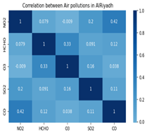
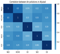
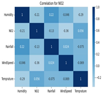
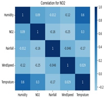
Moreover, to investigate the correlation among these pollutants we used the Pearson correlation coefficient which measures the linear correlation between two datasets. Its value usually ranges from -1 (high negative correlation) to 1 (high positive correlation). A value closer to zero indicates a weaker or non-existent linear relationship. By calculating the Pearson correlation coefficient, we aimed to determine whether these pollutants have a direct or inverse relationship, indicating whether they increase or decrease together. In addition, we calculated the correlations between pollutant NO₂ and meteorological features such as temperature and humidity to conduct further analysis on this pollutant. We have two reasons to select this pollutant specifically. First, we noted in our results that all the pollutants have the highest concentration in the industrial city except NO₂, hence we investigated its correlation to the weather data. Second, we noticed that all the pollutants show approximately the same trend in their correlation with weather parameters, so see that it is sufficient to present only one of these pollutants.
In addition to studying the correlation between air pollutants, we also used the heat map method to visualize spatial variations in pollutant concentrations and meteorological characteristics during all the months of the years 2022 and 2023.
A crucial aspect of the analysis involved using a two-way analysis of variance (ANOVA) to assess the effects of city and year on air pollutant levels. Two-way ANOVA is a powerful statistical technique that simultaneously examines two independent variables and their interaction with a dependent variable. In this study, the independent variables were city and year, while the dependent variables were the five air pollutants. By utilizing two-way ANOVA, we will be able to determine whether the city or year had a significant impact on air pollution levels and whether there was an interaction between these two factors. This analysis provided valuable insights into the relative contributions of city-specific characteristics and temporal trends to air quality variations. The two-way ANOVA variables were described as follows:
- City: City characteristics (industrial, agricultural, and population density)
- Year: Recording the reading of every pollutant in the city during (2022-2023)
- Air pollutants: The concentration of pollutants in any city varies during the year.
- Then the null and alternative hypotheses are determined:
- Null Hypothesis (H0): There is no significant difference in the mean pollution levels among the three cities.
- Alternative Hypothesis (H1): There is a significant difference in the mean pollution levels among the three cities.
3.4. Methods of Predictive Modeling
This section will present the methods we used to build the models and their evaluation.
3.4.1. Models’ Development
To develop and evaluate the proposed model, we used a data-splitting strategy to evaluate the prediction performance unbiasedly [44]. The dataset was split into two sets: a training set with 90% and a test set with 10% of the data. The training set was used to train the model, and the test set to evaluate accuracy.
The primary objective of this research was to propose a supervised learning approach to develop a deep learning model capable of predicting NO₂ concentration with minimal error across various metrics. As demonstrated in previous research, LSTM models have shown promising results in air pollution prediction [34]. This encourages our research to focus on the LSTM model. Moreover, LSTM outperforms RNN’s ability to store large amounts of prior time-series data without the vanishing gradient problem [24].
Additionally, we used multiple hyperparameters to achieve the best performance in a reasonable time. All models are similar in batch size of parameters (32), activation function (ReLu), and the mean square error (MSE) was used as a loss function to measure the error rate between the actual and predicted values but differ in the number of layers and number of neurons per layer as shown in Table 2. Moreover, we adjusted the sliding window parameters (window size, step size, and features). All hyperparameters are adjusted to improve the performance during the experimental process. For a 5-day ahead prediction, we used a window size of 14 days, considering the influence of the past 14 days’ weather and pollution data. The step size was set to 5 days, and the features included temperature, wind speed, rainfall, humidity, and NO₂ concentration. These features served as input variables to the model for multi-step prediction. Studies have shown that vector representation of time using Time2Vec with the LSTM model improves performance in most cases and never leads to a deterioration in prediction performance [26]. We used it with the optimized model, which gave better prediction results. All these hyperparameters were used with the models that were developed in this research.
In this study, we conducted three experiments to verify the effectiveness of the proposed model. Each experiment focused on evaluating a different aspect. The first experiment used the LSTM algorithm, which has shown promising results in predicting air pollution [34]. In the second experiment, we improved the LSTM model using the Batch Normalization method, which is used to Normalize inputs of neural network layers by re-centering and re-gradients for faster, stable training [45]. The last experiment included embedding a Time2Vec layer to the improved LSTM model, which is important to verify whether our proposed framework performs well in predicting the NO₂ concentration in the air to make the prediction results more accurate and stable.
3.4.2. Evaluation of Metrics of Prediction Models
The training set is for model training, test set is for evaluating the performance and accuracy of the model. Different statistical measures were used to measure the distance between the actual values and the predicted values, including the mean absolute error (MAE) [46], the root mean square error (RMSE) [47], and the mean absolute percentage error (MAPE) [48]. These metrics are used to compare the predictive performance of the models across the three cities. These metrics can be defined as follows:
where y is the actual value, is the predicted value, i is the sample index, and n is the total number of samples, which is the length of the test set.
4. Results and Discussion
4.1. Results of the Descriptive Analysis
Table 3 summarizes the aggregated data, presenting the average and standard deviation of air pollutant levels across the three cities for the years 2022 and 2023. In addition, the correlations between the pollutants for the years 2022 and 2023 are presented in Table 4. The calculated correlations between pollutant NO₂ and meteorological features are presented in Table 5. Heat maps illustrating the spatial patterns of pollutants and meteorological variables across all months of 2022 and 2023 are presented in Table 6.
Given the nature of the three cities, some of the results are reasonable. Al Jubail is an industrial city, and it is known that one of the main sources of pollutants is manufacturing. Additionally, Al Riyadh is a city with a high population compared to other Saudi cities and has experienced significant urbanization in recent years. Najran is an agricultural city, which may contribute to lower pollution levels. Consequently, the mean levels of all pollutants are higher in Al Jubail and Al Riyadh, than in Najran. As shown in Figure 3, the average concentration of NO₂ is recorded as the highest average in Riyadh, followed by Jubail and then Najran. Al Riyadh has higher NO₂ levels than Al Jubail by 39% in 2023 and 43% in 2022. We will present further analysis of this pollutant later using the correlation. Another notable point is that the mean levels of all pollutants in the three cities are higher in 2023 than in 2022, except for O₃.
In the following, we will summarize the main points we noted from the collected data:
- The humidity in Al Jubail is high, especially in the months from June to November.
- The wind speed in Al Jubail is higher than in the other two cities.
- NO₂ is the only pollutant that is higher in AL Riyadh than Al Jubail and it is especially higher during October.
- SO₂ has the highest mean in Al Jubail, and it is distributed throughout the year.
- Most of the emissions of HCHO in the three cities occurred from June to September.
- Most of the emissions of CO in the three cities in the year 2022 occurred in March.
- Most of the emissions of O₃ in the three cities occurred from April to September.
- In Al Riyadh, there is a positive linear relationship between NO₂ and CO, which is stronger in 2023.
- In Al Jubail there is a positive linear relationship between HCHO and NO₂ and between HCHO and SO₂.
- In Najran there is a negative linear relationship between O₃ and CO.
We have presented the correlation of NO₂ with meteorological parameters because we noticed a similar trend in the correlation between each pollutant and meteorological parameters. Additionally, we noted that NO₂ differs from all other pollutants, as it has a higher value in Al Riyadh than in Al Jubail. The correlation is presented in Table 5. These are the main points that can be concluded from the table:
- There is a moderate positive linear relationship between NO₂ and the temperature in Al Jubail and Najran.
- There is a moderate negative relationship between NO₂ and wind speed, but this relation is weak in Najran.
- There is a moderate negative relationship between NO₂ and humidity in Al Riyadh, despite the generally dry weather in the city.
The above results agree with research conducted in other areas of the world [49,50]. The major sources of NO₂ and volatile organic compounds (VOCs), including HCHO, are the large number of vehicles and emissions from industrial and chemical manufacturing [49]. Given the high levels of NO₂ in Al Riyadh, it can be attributed to the large number of vehicles, which is likely due to the high population. Using the EPA Multiscale Air Quality Model, Li et al. [51] researchers analyzed the relationship between several atmospheric parameters and NO₂ using observed concentrations from ground stations and satellites. They found that boundary layer height, wind speed, temperature, and relative humidity were the most important variables in determining the variation of NO₂ near the surface. In their results, NO₂ concentration was positively correlated with temperature and negatively correlated with wind speed.
Therefore, weather parameters play a crucial role in air quality monitoring. Based on the results in Table 5, we can conclude that the impact of weather parameters on NO₂ concentration varies across cities due to differing urban characteristics. In Najran, temperature and humidity have the strongest influence, with temperature inversely related to NO₂ and humidity positively correlated. While, in Al Jubail, temperature and wind speed are the primary factors affecting NO₂ concentration, with temperature positively correlated and wind speed negatively correlated. In Al Riyadh, wind speed and humidity are the most significant weather parameters, both inversely related to NO₂ concentration, meaning that increasing humidity and wind speed lead to decreased NO₂ levels. These findings are important to develop the model that will forecast the concentration of NO₂ to include the most important weather factors.
These weather parameters will have varying degrees of influence when training a prediction model for each city. Therefore, using a model trained on Al Riyadh data to predict NO₂ levels in Al Jubail, for instance, would be inappropriate, as we will demonstrate in our predictive modeling study. Furthermore, our experiments with transfer learning, where a model trained on Al Riyadh data is further trained on Al Jubail data, did not yield any significant improvement in predictive performance.
When we find a positive linear relationship between two pollutants, this may suggest similar sources for these pollutants. We find this positive relation in Al Riyadh between NO₂ and CO and between HCHO and O₃. The pollution in this case may be attributed to the large number of vehicles and the extensive construction activities. In Al Jubail, there is a positive relation between NO₂ and SO₂, between and HCHO, as well as between HCHO and SO₂. The pollution in this case may be attributed to the emissions from industrial activities. In Najran there is a negative relation between O₃ and CO. Given that these two pollutants have the lowest levels in Najran in comparison to Al Riyadh and Al Jubail, and based on this study [50], when CO is present, it can react with O₃, forming CO and reducing the amount of O₃ available. Additionally, CO can absorb sunlight, which is essential for O₃ formation. As a result, high levels of CO can limit O₃ production in the atmosphere, creating a negative correlation between the two pollutants.
After that, all data processing and ANOVA testing for air pollutants (NO₂, SO₂, CO, O₃, HCHO) for the years (2022 and 2023) are carried out in three cities in the Kingdom classified (Industrial, Agricultural, and High Population) using the Python programming language. Next, an ANOVA will partition the total variance for each pollutant into three components: the main effect of the independent factor of city, the main effect of the independent factor of year, and the interaction effect of city and year. By means calculations, standard errors of the means (SEM statistic), P-value, and F-value were calculated for each factor. If the p-value obtained from the ANOVA is less than the significance level you chose (for example, alpha = 0.05), you can reject the null hypothesis. If the null hypothesis is rejected, this indicates that there are statistically significant differences in the average levels of pollution between the three cities during the two years.
As shown in Table 7, the probability values from the two-way ANOVA test for all air pollutants show the identification of the interaction effect between the independent factors and the dependent factors. For example, we find that the NO₂ pollutant has a significant main effect on the “City” factor (p-value = 3.773028 ) and that there is a relationship between the city characteristics and the concentration rate of the c pollutant. This means there are differences in the dependent factor across levels of the independent factor. Likewise, the lack of a significant main effect for the independent “Year” factor (p-value=9.665494 ) indicates that levels of this factor are associated with significant changes in NO₂ levels.
As for the dependent factor sulfur dioxide (SO₂) and its relationship with the “City” and “Year” variables, it was found that the “City” factor has a significant effect on the SO₂ concentration, as proven by the low probability value (P-value = 8.263521 ), and this indicates a significant difference in SO₂ concentration between the cities analyzed. In addition, the “Year” factor also shows no significant effect on SO₂ concentration and has a high P value (P-value = 1.547905 ). In summary, the ANOVA analysis reveals that the “City” factor has a stronger effect, while the “Year” factor shows a weaker effect on SO₂ concentration. However, as for the dependent factor carbon oxide (CO), a significant difference and effect was found with the two variables “city” and “year,” based on their probability values less than alpha. We find that the ozone pollutant (O₃) is affected by the city’s independent factor and has a probability value less than alpha, which is (p-value = 1.269544 ). This indicates a relationship between the city’s characteristics and the concentration rate of the O₃ pollutant. It also has a lower probability value with the independent “year” factor (p-value = 3.492794 ), which leads to the fact that the year and city factors have a relatively considerable influence on the O₃ concentration rate in the air. As for the last pollutant, which is HCHO, we find that it is also affected by the independent factor of the city, as there is a relationship between the characteristics of the city and the rate of increase or decrease in the concentration of HCHO in the air. It is also affected by the independent “Year” factor.
4.2. Results of Predictive Modeling
This paper has selected NO₂ as an important air pollutant that poses a threat to human health and the environment. It is produced by the burning of fossil fuels emitted from traffic and factories, and short and long-term exposure to these emissions can cause health problems [52]. Four atmospheric parameters were selected as input indicators, namely wind speed, temperature, humidity, and precipitation, in addition to the NO₂ concentration itself. To measure the relationship between the observed and predicted concentrations of NO₂, the performance of the three models was evaluated after training and testing the models on the datasets using three criteria including RMSE, MAE, and MAPE, and the results are recorded in Table 8. As shown in the table, the addition of batch normalization in the improved model produces a slight improvement in the forecasting quality as lower metric values indicate a smaller distance between predicted and actual NO₂ levels. Furthermore, incorporating a Time2Vec layer to capture temporal patterns led to a significant enhancement in prediction quality, as demonstrated in Table 8 and Figure 4. Figure 4 shows a graphical representation of the predicted and observed concentrations of nitrogen dioxide in the three cities using the proposed model. These concentrations showed a strong correlation with each other for nitrogen dioxide. These results indicate that the proposed model outperformed the prediction performance of the models without using Time2Vec. This demonstrates that including the time vector can improve the prediction performance and is an effective approach to improving the accuracy of atmospheric pollutant concentration prediction.
Training and validation loss curves for the three cities are shown in Figure 5 and Figure 6. Figure 5 depicts the case using the optimized LSTM model without Time2Vec, while Figure 6 illustrates the curves after incorporating Time2Vec into the improved model. These curves indicate that neither overfitting nor underfitting occurred during training.
Figure 7 shows a graph of the absolute prediction error of the predicted and true NO₂ values in the test phase for all three cities. Each box represents the average air pollution level for each month. Based on the graph, we can make the following observations:
- In Najran prediction accuracy varies with the mean absolute error, with the model having the greatest difficulty accurately predicting nitrogen concentration during May and August, with the highest mean absolute errors. March and December have lower mean absolute errors, indicating that the model performed better at predicting nitrogen concentration during these months.
- In Al Riyadh, the highest mean absolute errors were recorded in March and September, indicating that the model had greater difficulty accurately predicting nitrogen concentrations during these months. The model performed better in forecasting in February and May.
- In Al Jubail the months of July and September have the highest mean error, indicating that the model had difficulty making predictions during these months. The months of January and June have the lowest mean absolute error, indicating that the model performed best during these months.
Figure 7.
The presentation Boxplot of Air Pollution for three cities should be listed as: (a) Al Jubail City; (b) Al Riyadh City; and (c) Najran City.
Figure 7.
The presentation Boxplot of Air Pollution for three cities should be listed as: (a) Al Jubail City; (b) Al Riyadh City; and (c) Najran City.
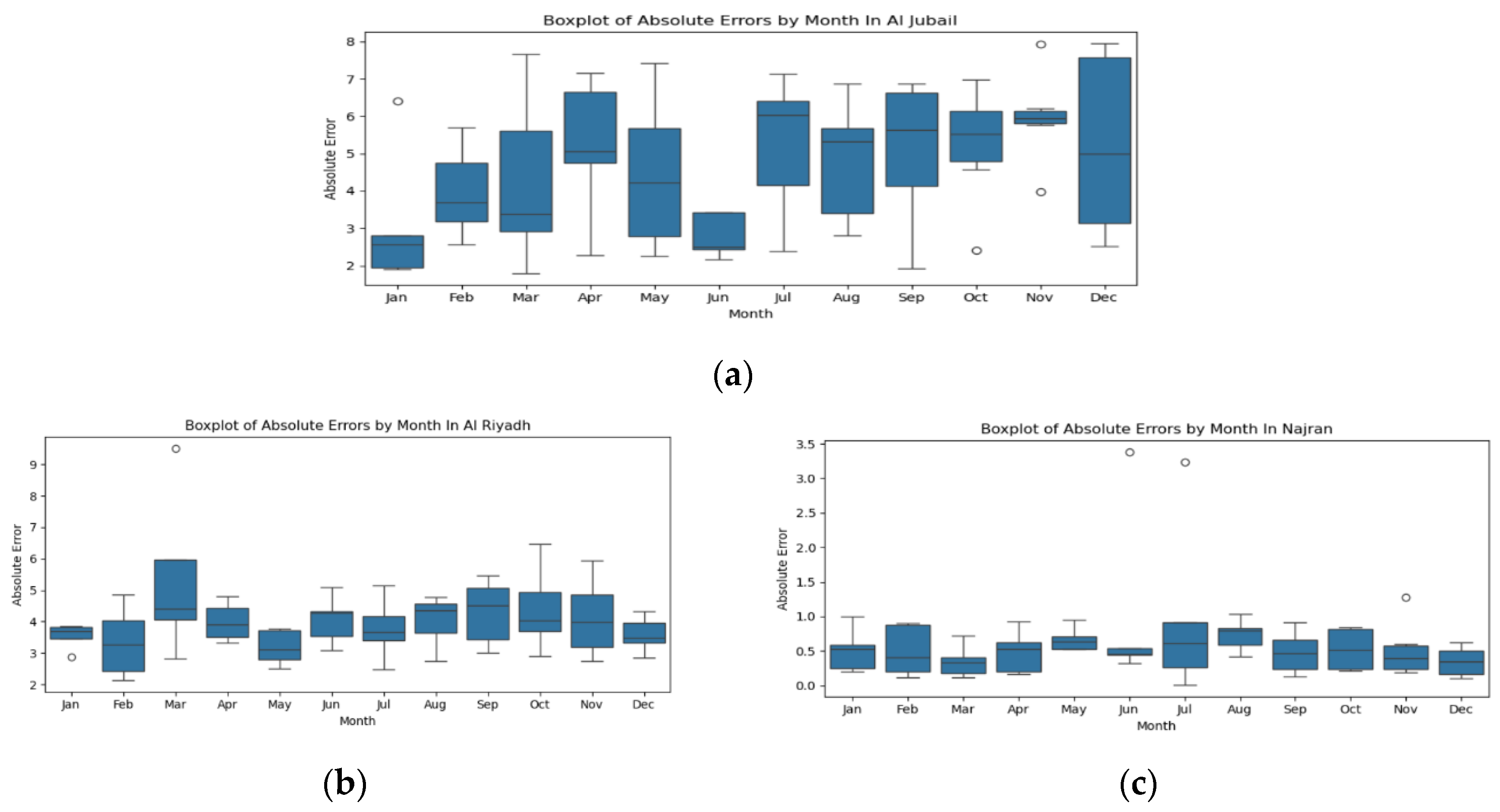
Moreover, we noticed a large variation in the mean error values in Al Riyadh compared to the other cities, especially during December, March, and May. This may indicate that the model makes larger errors with higher concentrations, which is expected when we use the mean squared error to calculate the loss function of the model during training. This is because the mean squared error loss function is sensitive to outliers, causing outliers to dominate the learning process. Consequently, we suggest that the selection of the loss function should depend on the existence of outliers in the data collected, given that these outliers are not errors but indicators of larger concentrations of the pollutant.
5. Conclusions
This study conducted a comprehensive analysis of air pollution in three Saudi Arabian cities: Al Riyadh, Al Jubail, and Najran, with distinct environmental characteristics. By utilizing Sentinel-5 satellite data and Google Earth Engine, we performed a descriptive analysis of air pollutant trends from 2022 to 2023 and developed a robust deep-learning model for NO₂ prediction.
Our descriptive analysis revealed significant variations in air pollutant levels across the three cities, highlighting the influence of industrial activities, population density, and meteorological factors. Notably, Al Jubail has the highest levels of most studied pollutants due to its industrial nature, while Al Riyadh showed elevated NO₂ concentrations likely attributed to traffic emissions. This study also confirmed a strong relationship between city characteristics and the rate of increase or decrease of air pollutants.
We developed a deep learning model using LSTM and embedding the Time2Vec algorithm to enhance air pollution monitoring and forecasting capabilities. This model demonstrated superior accuracy in predicting NO₂ concentrations compared to traditional LSTM models, effectively capturing temporal patterns and achieving minimal prediction errors. The integration of Time2Vec proved particularly valuable in improving prediction quality. The developed deep learning framework can be a useful tool for local authorities and environmental agencies in Saudi Arabia to enhance their air quality monitoring and forecasting capabilities. By providing accurate predictions, this framework can support the implementation of careful measures to reduce air pollution, such as traffic management, industrial emission controls, and public awareness campaigns.
The study offers insights into air pollution dynamics and forecasting but has limitations. First, the study used data from a single satellite air quality monitoring station; it recommends using ground monitoring stations with diverse emission sources to achieve more effective planning of air quality management strategies. Second, NO₂ levels in urban areas are closely related to traffic composition and flow, which calls for their characteristics to be included in detail in future models and work.
Acknowledgments
The guest editors of this special issue of the International Journal of Environmental Research and Public Health are grateful to all the authors, reviewers, and MDPI staff.
Conflicts of Interest
The authors declare no conflict of interest.
References
- World Health Organization. (2021). Human health effects of polycyclic aromatic hydrocarbons as ambient air pollutants: report of the Working Group on Polycyclic Aromatic Hydrocarbons of the Joint Task Force on Health Aspects of Air Pollution. World Health Organization. Regional Office for Europe. (Air Pollution: A Study of Its Concept, Causes, Sources and Effects. Asian Journal of Water, Environment and Pollution).
- Al-Taai SHH, Mohammed al-Dulaimi WA. Air Pollution: A Study of Its Concept, Causes, Sources and Effects. Asian J Water Environ Pollut. 2022;19:17–22.
- Canha N, Diapouli E, Almeida SM. Integrated human exposure to air pollution [Internet]. Int. J. Environ. Res. Public. Health. MDPI; 2021 [cited 2024 Dec 11]. p. 2233. Available online: https://www.mdpi.com/1660-4601/18/5/2233.
- Ng CFS, Hashizume M, Obase Y, Doi M, Tamura K, Tomari S, et al. Associations of chemical composition and sources of PM2.5 with lung function of severe asthmatic adults in a low air pollution environment of urban Nagasaki, Japan. Environ Pollut. 2019;252:599–606.
- Yang D, Wang J, Yan X, Liu H. Subway air quality modeling using improved deep learning framework. Process Saf Environ Prot. 2022;163:487–97.
- Alsaud AB, Yas H, Alatawi A. A New Decision-Making Approach for Riyadh makes up 50 percent of the non-oil economy of Saudi Arabia. J Contemp Issues Bus Gov. 2021;27:3376–92.
- Mujabar S, Rao V. Estimation and analysis of land surface temperature of Jubail Industrial City, Saudi Arabia, by using remote sensing and GIS technologies. Arab J Geosci. 2018;11:742.
- Abd El Aal AK, Kamel M, Alyami SH. Environmental Analysis of Land Use and Land Change of Najran City: GIS and Remote Sensing. Arab J Sci Eng. 2020;45:8803–16.
- Kazemi Garajeh M, Blaschke T, Hossein Haghi V, Weng Q, Valizadeh Kamran K, Li Z. A Comparison between Sentinel-2 and Landsat 8 OLI Satellite Images for Soil Salinity Distribution Mapping Using a Deep Learning Convolutional Neural Network. Can J Remote Sens. 2022;48:452–68.
- Loyola DG, Gimeno García S, Lutz R, Argyrouli A, Romahn F, Spurr RJ, et al. The operational cloud retrieval algorithms from TROPOMI on board Sentinel-5 Precursor. Atmospheric Meas Tech. 2018;11:409–27.
- Vîrghileanu M, Săvulescu I, Mihai B-A, Nistor C, Dobre R. Nitrogen Dioxide (NO2) Pollution monitoring with Sentinel-5P satellite imagery over Europe during the coronavirus pandemic outbreak. Remote Sens. 2020;12:3575.
- Mukundan A, Huang C-C, Men T-C, Lin F-C, Wang H-C. Air pollution detection using a novel snap-shot hyperspectral imaging technique. Sensors. 2022;22:6231.
- Haque MN, Sharif MS, Rudra RR, Mahi MM, Uddin MJ, Abd Ellah RG. Analyzing the spatio-temporal directions of air pollutants for the initial wave of COVID-19 epidemic over Bangladesh: Application of satellite imageries and Google Earth Engine. Remote Sens Appl Soc Environ. 2022;28:100862.
- Ghasempour F, Sekertekin A, Kutoglu SH. Google Earth Engine based spatio-temporal analysis of air pollutants before and during the first wave COVID-19 outbreak over Turkey via remote sensing. J Clean Prod. 2021;319:128599.
- Al-Alola SS, Alkadi II, Alogayell HM, Mohamed SA, Ismail IY. Air quality estimation using remote sensing and GIS-spatial technologies along Al-Shamal train pathway, Al-Qurayyat City in Saudi Arabia. Environ Sustain Indic. 2022;15:100184.
- Ul-Haq Z, Batool SA, Tariq S, Rana AD, Mahmood K, Chaudhary MN, et al. TEMPORAL AND SPATIAL VARIATIONS OF NO 2 OVER SAUDI ARABIA AND IDENTIFICATION OF MAJOR HOTSPOT AREAS DURING 2005-2014 BY USING SA℡LITE DATA. Appl Ecol Environ Res [Internet]. 2018 [cited 2024 Dec 11]; 16. Available online: https://aloki.hu/pdf/1605_57575770.pdf.
- Salman A, Al-Tayib M, Hag-Elsafi S, Zaidi FK, Al-Duwarij N. Spatiotemporal assessment of air quality and heat island effect due to industrial activities and urbanization in Southern Riyadh, Saudi Arabia. Appl Sci. 2021;11:2107.
- Farahat A, Chauhan A, Al Otaibi M, Singh RP. Air Quality Over Major Cities of Saudi Arabia During Hajj Periods of 2019 and 2020. Earth Syst Environ. 2021;5:101–14.
- Alharbi NH, Alharthi ZS, Alanezi NA, Syed L. Spatial Analysis of COVID 19 in KSA Related to Air Pollution Factor. In: Sheikh YH, Rai IA, Bakar AD, editors. E-Infrastruct E-Serv Dev Ctries [Internet]. Cham: Springer International Publishing; 2022 [cited 2024 Dec 11]. p. 443–57. Available online: https://link.springer.com/10.1007/978-3-031-06374-9_29.
- Hassan R, Rahman M, Hamdan A. Assessment of air quality index (AQI) in Riyadh, Saudi Arabia. IOP Conf Ser Earth Environ Sci [Internet]. IOP Publishing; 2022 [cited 2024 Dec 11]. p. 012003. Available online: https://iopscience.iop.org/article/10.1088/1755-1315/1026/1/012003/meta.
- Precious DH, Ogunrombi TS, Otunuya OJ. Design Of Modular Program For Evaluation Of Visibility Time Of Satellite With Highly Eccentric Orbit. J Multidiscip Eng Sci Res JMESR [Internet]. 2022 [cited 2024 Dec 11];1. Available online: https://www.researchgate.net/profile/Tijesuni-Ogunrombi/publication/365761565_Design_Of_Modular_Program_For_Evaluation_Of_Visibility_Time_Of_Satellite_With_Highly_Eccentric_Orbit/links/6381dda048124c2bc671d2d7/Design-Of-Modular-Program-For-Evaluation-Of-Visibility-Time-Of-Satellite-With-Highly-Eccentric-Orbit.pdf.
- Ebenezer, G. The Role of Meteorology in Atmospheric Processes and Air Pollution Studies. Dec 0–14 [Internet]. 2019 [cited 2024 Dec 11]. Available online: https://www.researchgate.net/profile/Godwin-Ebenezer-2/publication/337889771_THE_ROLE_OF_METEOROLOGY_IN_ATMOSPHERIC_PROCESSES_AND_AIR_POLLUTION_STUDIES/links/5df0cea3a6fdcc283717cb0c/THE-ROLE-OF-METEOROLOGY-IN-ATMOSPHERIC-PROCESSES-AND-AIR-POLLUTION-STUDIES.pdf.
- Jutz S, Milagro-Perez MP. Copernicus: the european earth observation programme. Rev Teledetec. 2020;V–XI.
- Mahmoud A, Mohammed A. A Survey on Deep Learning for Time-Series Forecasting. In: Hassanien AE, Darwish A, editors. Mach Learn Big Data Anal Paradig Anal Appl Chall [Internet]. Cham: Springer International Publishing; 2021 [cited 2024 Dec 11]. p. 365–92. Available online: http://link.springer.com/10.1007/978-3-030-59338-4_19.
- Pratt T, Allnutt JE. Satellite communications [Internet]. John Wiley & Sons; 2019 [cited 2024 Dec 11]. Available online: https://books.google.com/books?hl=ar&lr=&id=atmxDwAAQBAJ&oi=fnd&pg=PR11&dq=%5B25%5D+T.+Pratt+and+J.+E.+Allnutt,+Satellite+communications.+John+Wiley+%26+Sons,+2019.&ots=7y8PsN03Kk&sig=DdjUb0QxMPtW0H93GytdeSZxWaU.
- Kazemi SM, Goel R, Eghbali S, Ramanan J, Sahota J, Thakur S, et al. Time2Vec: Learning a Vector Representation of Time [Internet]. arXiv; 2019 [cited 2024 Dec 11]. Available online: http://arxiv.org/abs/1907.05321.
- Sun X, Xu W, Jiang H, Wang Q. A deep multitask learning approach for air quality prediction. Ann Oper Res. 2021;303:51–79.
- Sermpinis G, Karathanasopoulos A, Rosillo R, De La Fuente D. Neural networks in financial trading. Ann Oper Res. 2021;297:293–308.
- Huang X, Qi J, Sun Y, Zhang R. Mala: Cross-domain dialogue generation with action learning. Proc AAAI Conf Artif Intell [Internet]. 2020 [cited 2024 Dec 11]. p. 7977–84. Available online: https://ojs.aaai.org/index.php/AAAI/article/view/6306.
- Kumar A, Singh JP, Dwivedi YK, Rana NP. A deep multi-modal neural network for informative Twitter content classification during emergencies. Ann Oper Res. 2022;319:791–822.
- Wang J, Zhang X, Guo Z, Lu H. Developing an early-warning system for air quality prediction and assessment of cities in China. Expert Syst Appl. 2017;84:102–16.
- Alzubaidi L, Zhang J, Humaidi AJ, Al-Dujaili A, Duan Y, Al-Shamma O, et al. Review of deep learning: concepts, CNN architectures, challenges, applications, future directions. J Big Data. 2021;8:53.
- Lu X-Q, Tian J, Liao Q, Xu Z-W, Gan L. CNN-LSTM based incremental attention mechanism enabled phase-space reconstruction for chaotic time series prediction. J Electron Sci Technol. 2024;22:100256.
- Utku A, Can Ü. Deep learning based air quality prediction: a case study for London. Türk Doğa Ve Fen Derg. 2022;11:126–34.
- Krishan M, Jha S, Das J, Singh A, Goyal MK, Sekar C. Air quality modelling using long short-term memory (LSTM) over NCT-Delhi, India. Air Qual Atmosphere Health. 2019;12:899–908.
- Li X, Zhong Y, Shang W, Zhang X, Shan B, Wang X. Total electricity consumption forecasting based on Transformer time series models. Procedia Comput Sci. 2022;214:312–20.
- Peñaloza, V. Time2Vec Embedding on a Seq2Seq Bi-directional LSTM Network for Pedestrian Trajectory Prediction. Res Comput Sci. 2020;149:249–60.
- Xu W, Wang Q, Chen R. Spatio-temporal prediction of crop disease severity for agricultural emergency management based on recurrent neural networks. GeoInformatica. 2018;22:363–81.
- Van Geffen J, Eskes H, Compernolle S, Pinardi G, Verhoelst T, Lambert J-C, et al. Sentinel-5P TROPOMI NO 2 retrieval: impact of version v2. 2 improvements and comparisons with OMI and ground-based data. Atmospheric Meas Tech. 2022;15:2037–60.
- de Bruyn NTM. Data assimilation of CrIS and TROPOMI satellite CO concentrations and its potential for constraining global OH [Internet] [PhD Thesis]. Carleton University; 2021 [cited 2024 Dec 11]. Available online: https://repository.library.carleton.ca/concern/etds/wh246t26t.
- Koukouli M-E, Skoulidou I, Karavias A, Parcharidis I, Balis D, Manders A, et al. Sudden changes in nitrogen dioxide emissions over Greece due to lockdown after the outbreak of COVID-19. Atmospheric Chem Phys. 2021;21:1759–74.
- Wang Y, Liu K, He Y, Fu Q, Luo W, Li W, et al. Research on Missing Value Imputation to Improve the Validity of Air Quality Data Evaluation on the Qinghai-Tibetan Plateau. Atmosphere. 2023;14:1821.
- Huang L, Qin J, Zhou Y, Zhu F, Liu L, Shao L. Normalization techniques in training dnns: Methodology, analysis and application. IEEE Trans Pattern Anal Mach Intell. 2023;45:10173–96.
- Joseph VR, Vakayil A. SPlit: An Optimal Method for Data Splitting. Technometrics. 2022;64:166–76.
- Guo M-H, Xu T-X, Liu J-J, Liu Z-N, Jiang P-T, Mu T-J, et al. Attention mechanisms in computer vision: A survey. Comput Vis Media. 2022;8:331–68.
- Muñoz DF, Ramírez-López A. A note on bias and mean squared error in steady-state quantile estimation. Oper Res Lett. 2015;43:374–7.
- Willmott CJ, Matsuura K. Advantages of the mean absolute error (MAE) over the root mean square error (RMSE) in assessing average model performance. Clim Res. 2005;30:79–82.
- Lam KF, Mui HW, Yuen HK. A note on minimizing absolute percentage error in combined forecasts. Comput Oper Res. 2001;28:1141–7.
- Khan RH, Quayyum Z, Rahman S. A quantitative assessment of natural and anthropogenic effects on the occurrence of high air pollution loading in Dhaka and neighboring cities and health consequences. Environ Monit Assess. 2023;195:1509.
- Gidarjati M, Matsumoto T. Correlation between meteorological variables, air quality, and the Coronavirus-19 pandemic events. Glob J Environ Sci Manag [Internet]. 2024 [cited 2024 Dec 11]. Available online: https://www.gjesm.net/article_713771.html.
- Li L, Wu J. Spatiotemporal estimation of satellite-borne and ground-level NO2 using full residual deep networks. Remote Sens Environ. 2021;254:112257.
- Ćurić M, Zafirovski O, Spiridonov V. Air Quality and Health. Essent Med Meteorol [Internet]. Cham: Springer International Publishing; 2022 [cited 2024 Dec 11]. p. 143–82. Available online: https://link.springer.com/10.1007/978-3-030-80975-1_8.
Figure 1.
Structure of the LSTM [24].
Figure 1.
Structure of the LSTM [24].
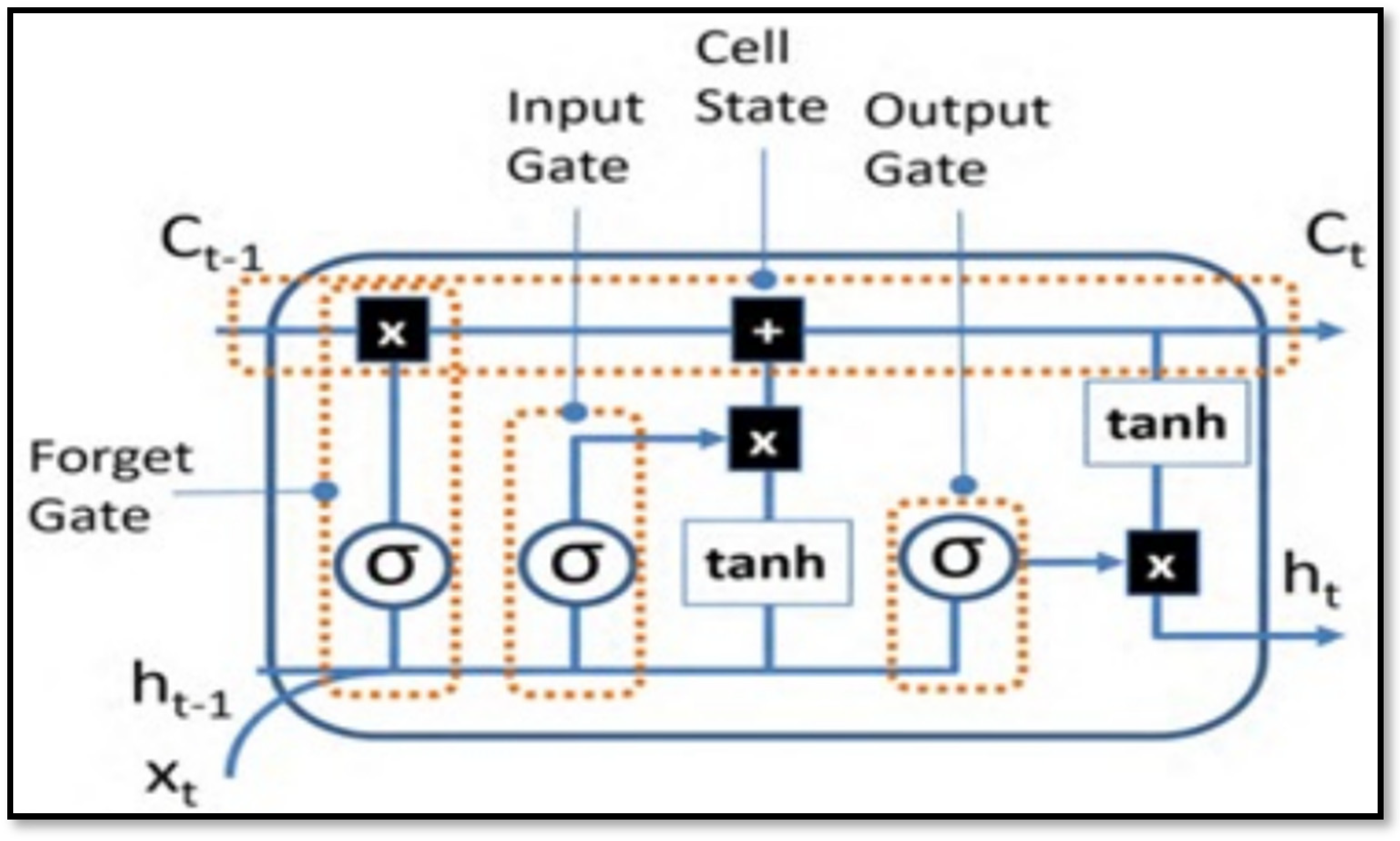
Figure 2.
Workflow for the proposed model.
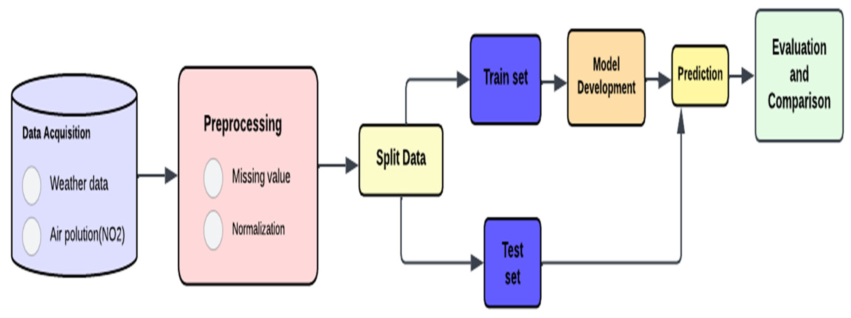
Figure 3.
Distribution of NO₂ concentration in the three cities.
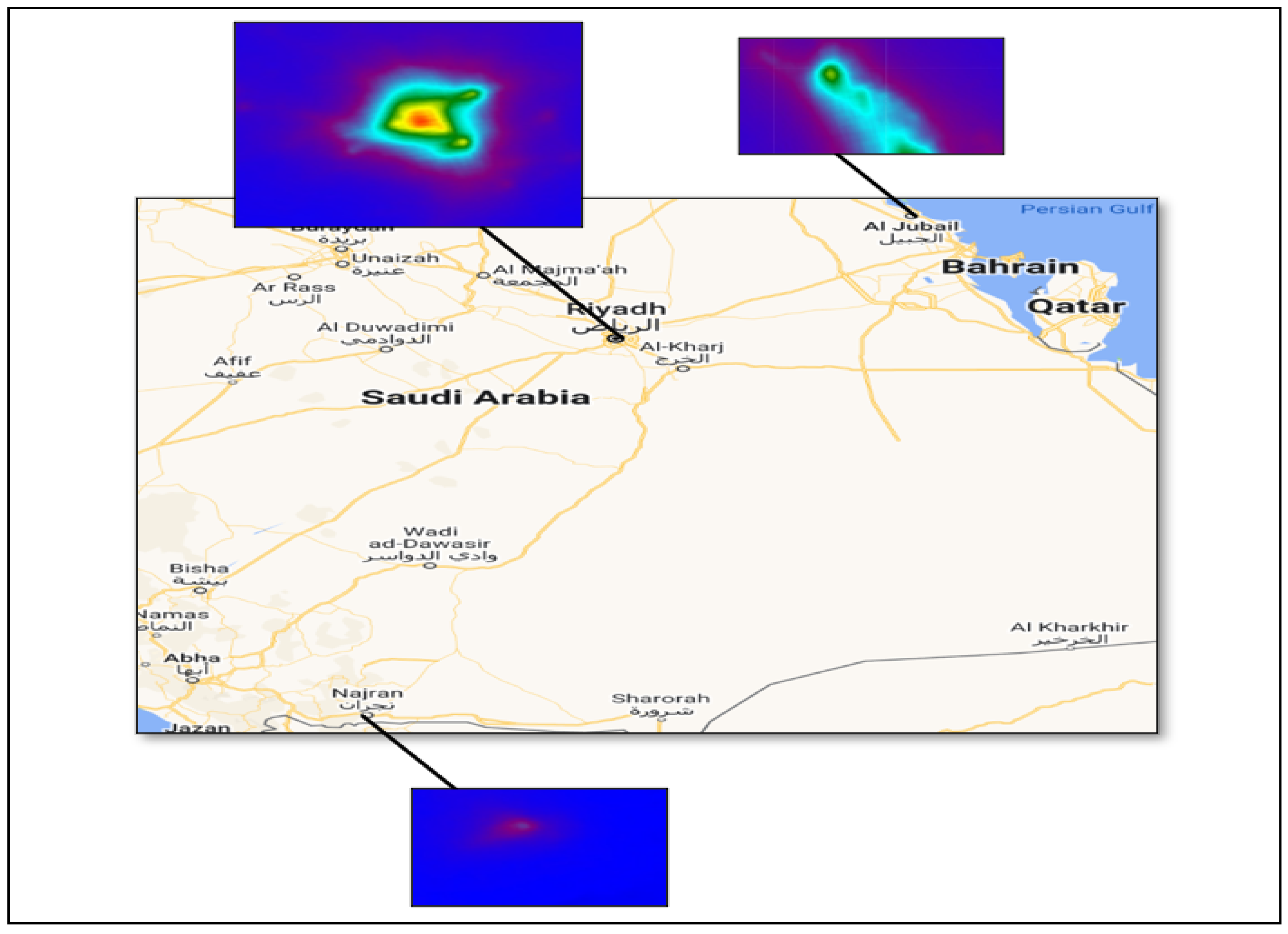
Figure 4.
Original and predicted values of nitrogen dioxide levels in the improved LSTM model with T2Vec for three cities. They should be listed as: (a) Al Jubail City; (b) Al Riyadh City; and (c) Najran City.
Figure 4.
Original and predicted values of nitrogen dioxide levels in the improved LSTM model with T2Vec for three cities. They should be listed as: (a) Al Jubail City; (b) Al Riyadh City; and (c) Najran City.
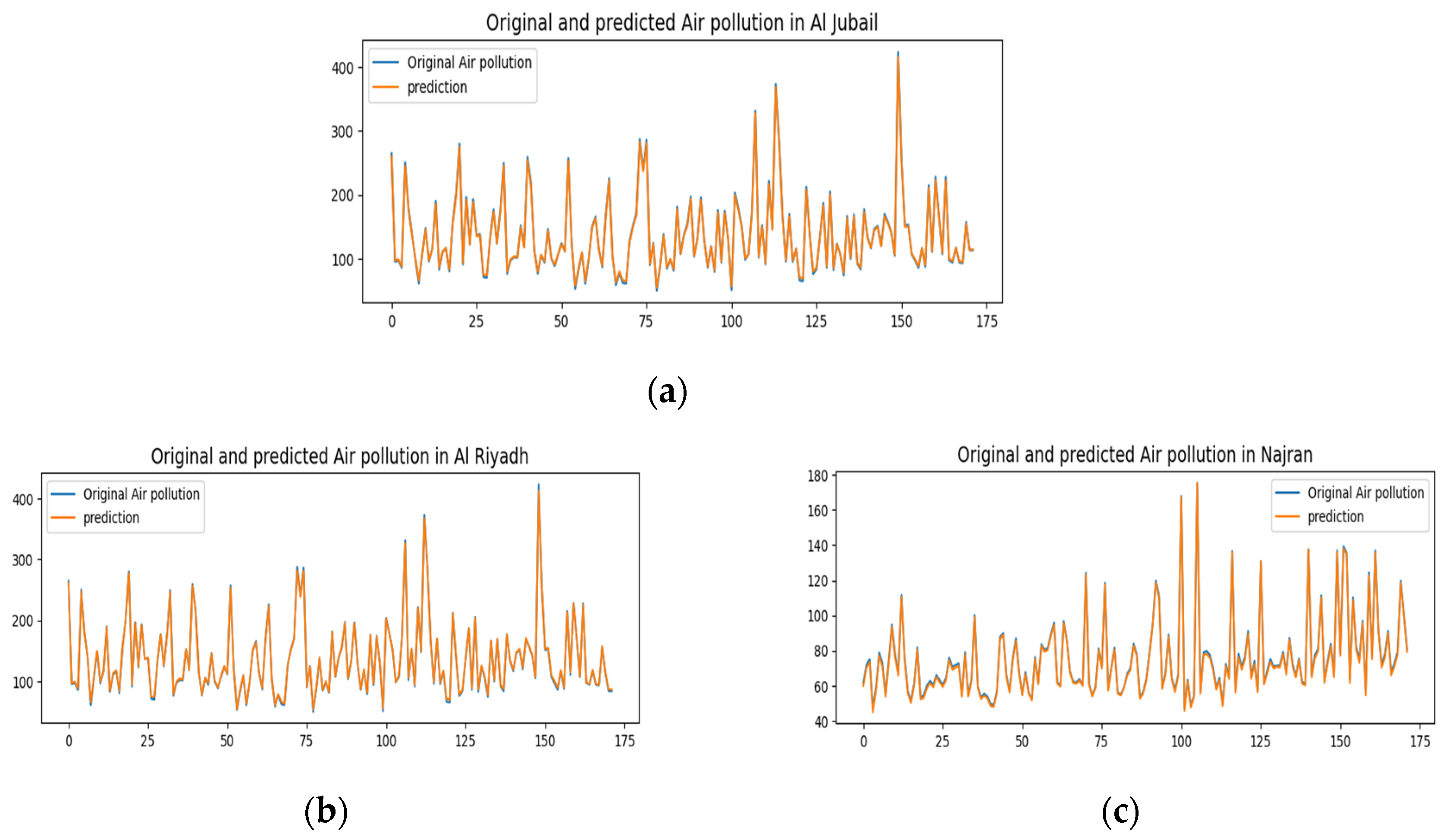
Figure 5.
Train and validation of the improved LSTM model for three cities should be listed as: (a) Al Jubail City; (b) Al Riyadh City; and (c) Najran City.
Figure 5.
Train and validation of the improved LSTM model for three cities should be listed as: (a) Al Jubail City; (b) Al Riyadh City; and (c) Najran City.
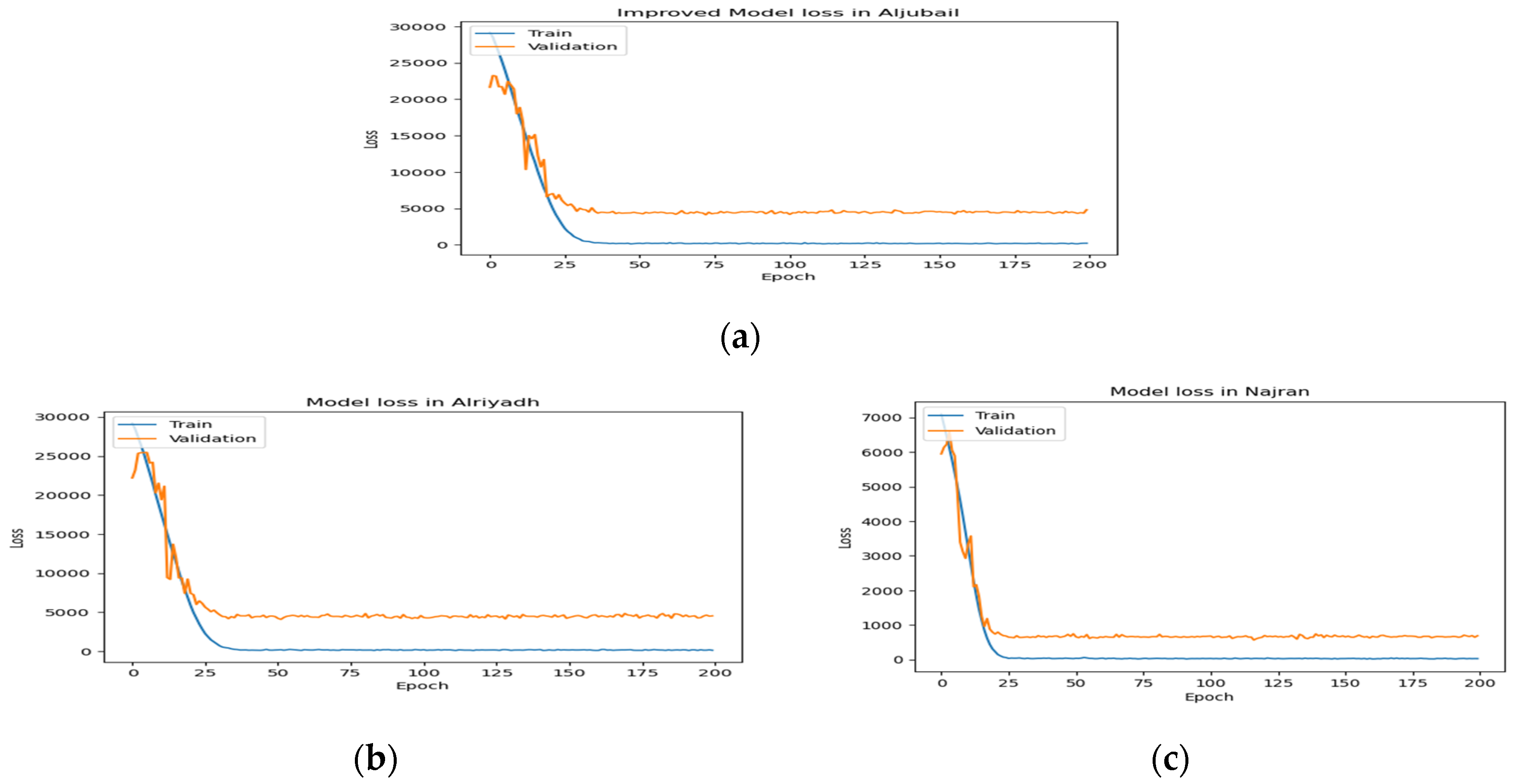
Figure 6.
Train and validation of the improved LSTM model with T2Vec for three cities should be listed as: (a) Al Jubail City; (b) Al Riyadh City; and (c) Najran City.
Figure 6.
Train and validation of the improved LSTM model with T2Vec for three cities should be listed as: (a) Al Jubail City; (b) Al Riyadh City; and (c) Najran City.
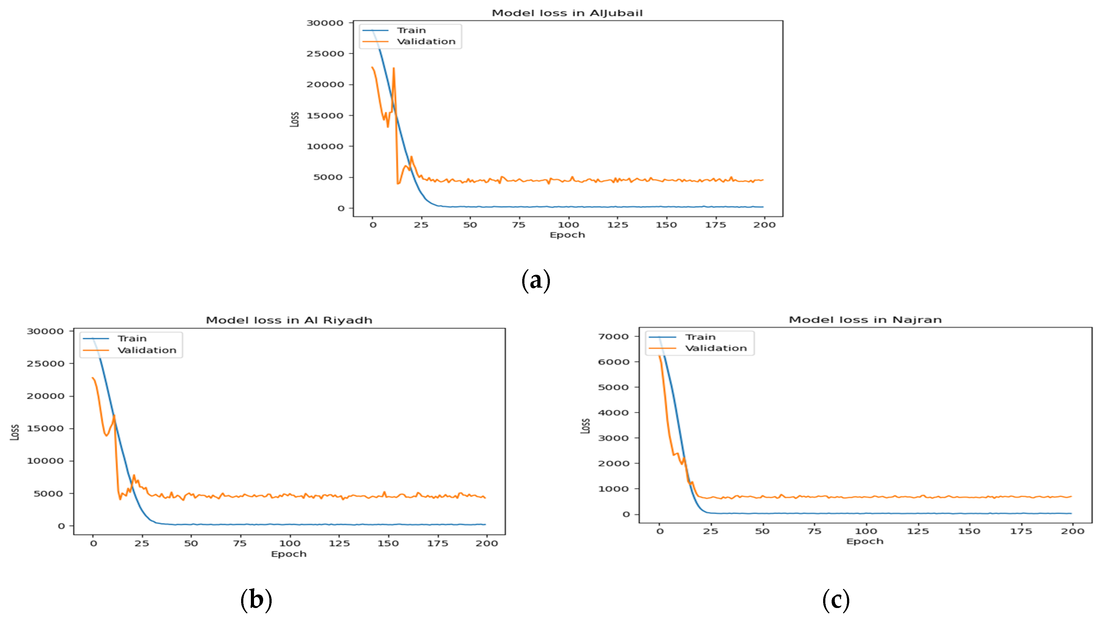

Table 1.
List of variables names and units.
| # | Variable |
|---|---|
| 1 | Relative humidity (%) |
| 2 | Rainfall (mm) |
| 3 | Temperature () |
| 4 | Wind speed (m/s) |
| 5 | NO₂ concentration (mg/) |
| 6 | SO₂ concentration (mg/) |
| 7 | HCHO concentration (mg/) |
| 8 | CO concentration (mg/) |
| 9 | O₃ concentration (mg/) |
Table 2.
List of hyperparameter values for models.
| Hyperparameters | LSTM | Improved LSTM | Proposed model |
|---|---|---|---|
| Number of Layers | 2 Layers | 3 Layers | 4 Layers |
| Layer (type) | 1-lstm_ (LSTM) 2-dense_ (Dense) |
1-lstm_ (LSTM) (Batch Normalization) 2-lstm_ (LSTM) (Batch Normalization) 3-dense_ (Dense) |
1-time2_vec (Time2Vec) 2-lstm_(LSTM) (Batch Normalization) 3-lstm_(LSTM) (Batch Normalization) 4-dense (Dense) |
| Number of Epochs | 100 | 200 | 200 |
| Number of Neurons per Layer | 100 | 50 | 50 |
Table 3.
These are tables of descriptive statistics of air pollutants in three target cities as follows: (a) Najran city; (b) Al Riyadh city and (c)Al Jubail city.
Table 3.
These are tables of descriptive statistics of air pollutants in three target cities as follows: (a) Najran city; (b) Al Riyadh city and (c)Al Jubail city.
| (a) | |||
|---|---|---|---|
| Air Pollutants | Year | Mean | Std |
| CO | 2022 | 27128.34 | 3291.96 |
| 2023 | 28294.89 | 2891.70 | |
| HCHO | 2022 | 87.627703 | 62.14 |
| 2023 | 95.129175 | 64.995 | |
| NO₂ | 2022 | 88.835017 | 33.097 |
| 2023 | 86.023103 | 28.09 | |
| , O₃ | 2022 | 120058.23 | 5867.48 |
| 2023 | 118408.20 | 6370.41 | |
| SO₂ | 2022 | 83.807 | 244.70 |
| 2023 | 111.05 | 248.75 | |
| (b) | |||
| Air Pollutants | Year | Mean | Std |
| CO | 2022 | 31550.50 | 3379.61 |
| 2023 | 31582.88 | 3038.82 | |
| HCHO | 2022 | 114.49 | 73.76 |
| 2023 | 121.99 | 69.35 | |
| NO₂ | 2022 | 263.29 | 169.86 |
| 2023 | 265.56 | 165.34 | |
| O₃ | 2022 | 123616.57 | 5957.60 |
| 2023 | 121498.27 | 5705.12 | |
| SO₂ | 2022 | 129.04 | 262.78 |
| 2023 | 130.72 | 309.46 | |
| (c) | |||
| Air Pollutants | Year | Mean | Std |
| CO | 2022 | 33643.41 | 3386.99 |
| 2023 | 34123.94 | 2920.209 | |
| HCHO | 2022 | 134.06 | 106.50 |
| 2023 | 156.81 | 114.71 | |
| NO₂ | 2022 | 183.03 | 86.55 |
| 2023 | 184.17 | 85.23 | |
| O₃ | 2022 | 125443.72 | 6258.49 |
| 2023 | 124113.17 | 5297.34 | |
| SO₂ | 2022 | 307.31 | 342.74 |
| 2023 | 334.10 | 393.97 | |
Table 4.
Correlation Matrices between Air pollutants.
| City\Year | 2022 | 2023 |
|---|---|---|
| Al Riyadh | 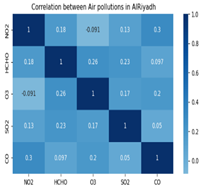 |
 |
| Al Jubail | 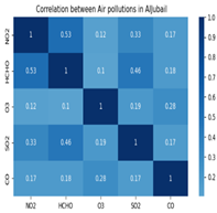 |
 |
| Najran | 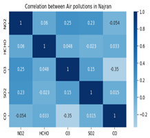 |
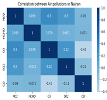 |
Table 5.
Correlation Matrices between NO₂ and meteorology in three cities.
| City\Year | 2022 | 2023 |
|---|---|---|
| Al Riyadh | 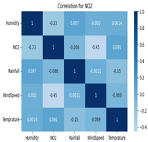 |
 |
| Al Jubail | 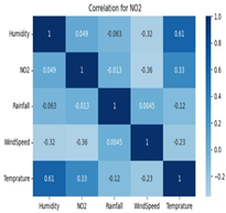 |
 |
| Najran | 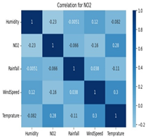 |
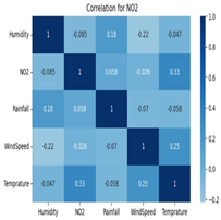 |
Table 6.
The heat map of metrological and Air pollutants as follows: (a) Temperature is measured in Celsius; (b) Humidity is measured in percentage; (c)Rainfall rate is measured in millimeters; (d)Wind speed is measured in meters per second; (e)NO₂ is measured in micrograms in each cubic meter of air; (f) SO₂ is measured in micrograms in each cubic meter of air; (g)CO is measured in micrograms in each cubic meter of air; (h)HCHO is measured in micrograms in each cubic meter of air; and (i) O₃ is measured in micrograms in each cubic meter of air.
| (a) | |
|---|---|
| City | Heatmap |
| Al Riyadh | 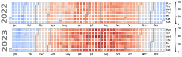 |
| Al Jubail | 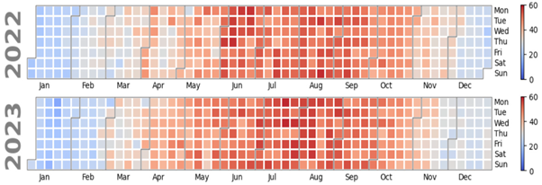 |
| Najran | 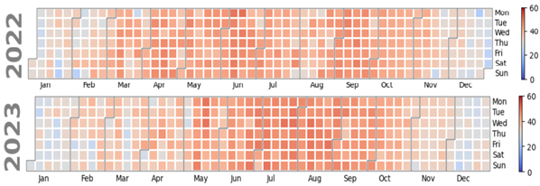 |
| (b) | |
| City | Heatmap |
| Al Riyadh | 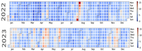 |
| Al Jubail | 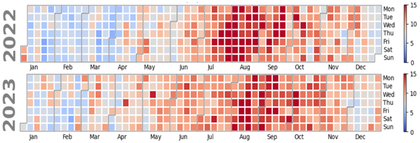 |
| Najran | 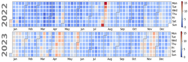 |
| (c) | |
| City | Heatmap |
| Al Riyadh | 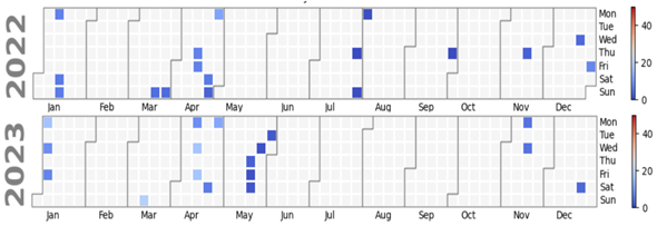 |
| Al Jubail |  |
| Najran | 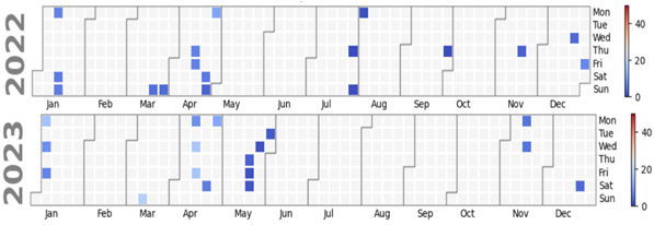 |
| (d) | |
| City | Heatmap |
| Al Riyadh | 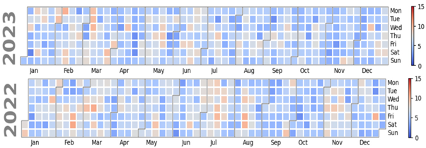 |
| Al Jubail | 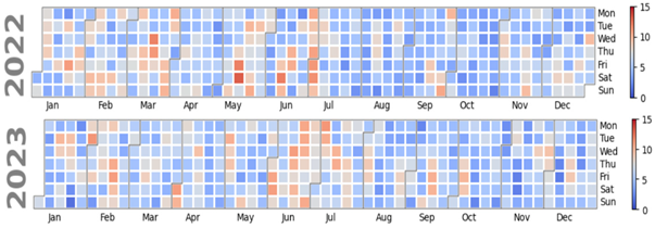 |
| Najran |  |
| (e) | |
| City | Heatmap |
| Al Riyadh | 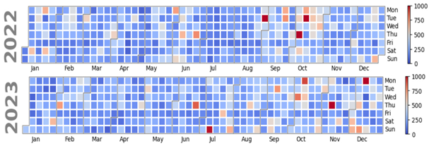 |
| Al Jubail | 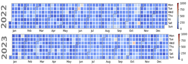 |
| Najran | 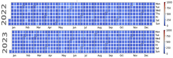 |
| (f) | |
| City | Heatmap |
| Al Riyadh | 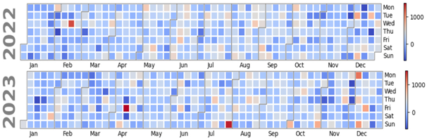 |
| Al Jubail | 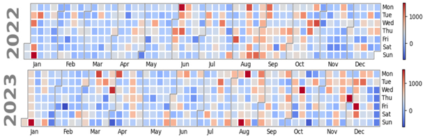 |
| Najran | 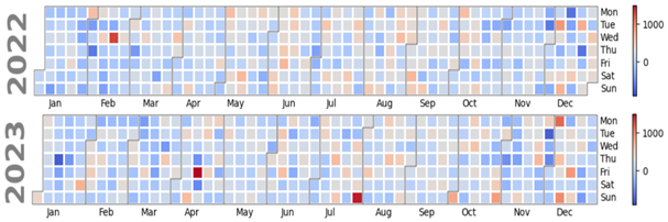 |
| (g) | |
| City | Heatmap |
| Al Riyadh | 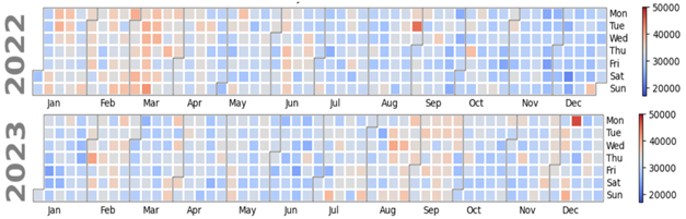 |
| Al Jubail | 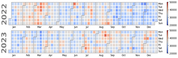 |
| Najran |  |
| (h) | |
| City | Heatmap |
| Al Riyadh | 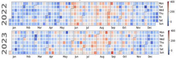 |
| Al Jubail | 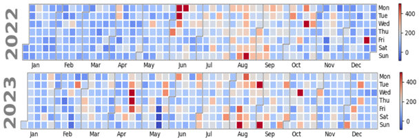 |
| Najran | 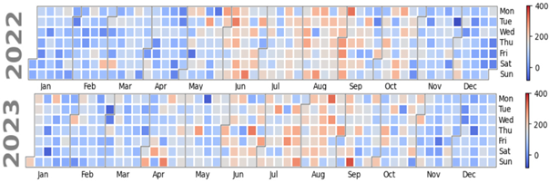 |
| (i) | |
| City | Heatmap |
| Al Riyadh | 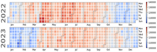 |
| Al Jubail | 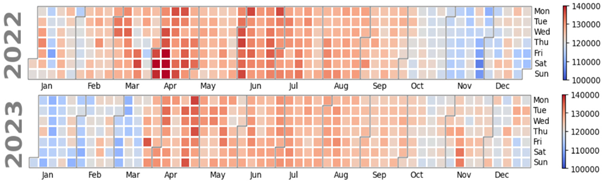 |
| Najran | 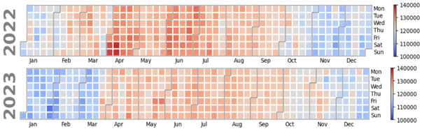 |
Table 7.
The probability values of the ANOVA study for all air pollutants.
| Air Pollutants | P-value of City | P-value of Year | P-value of City: Year |
|---|---|---|---|
| NO₂ | 3.773028 | 9.665494 | 8.986223 |
| SO₂ | 8.263521 | 1.547905 | 6.575841 |
| CO | 1.269544 | 3.492794 | 2.597570 |
| O₃ | 2.038939 | 2.347031 | 4.416942 |
| HCHO | 4.151673 | 5.022649 | 1.379713 |
Table 8.
Evaluation metrics for the three cities using the three prediction models. The improved model used batch normalization while the proposed model added a layer on Time2Vec.
Table 8.
Evaluation metrics for the three cities using the three prediction models. The improved model used batch normalization while the proposed model added a layer on Time2Vec.
| Model | Al Riyadh | Al Jubail | Najran | ||||||
|---|---|---|---|---|---|---|---|---|---|
| MAE | RMSE | MAPE | MAE | RMSE | MAPE | MAE | RMSE | MAPE | |
| LSTM | 42.77 | 55.91 | 33.75 | 42.97 | 55.83 | 33.98 | 15.10 | 22.28 | 19.62 |
| Improve LSTM | 42.07 | 54.74 | 33.43 | 42.23 | 55.15 | 32.76 | 14.92 | 21.79 | 19.24 |
| Proposed Model | 41.57 | 54.44 | 33.07 | 41.29 | 54.13 | 31.57 | 14.34 | 20.90 | 18.71 |
Disclaimer/Publisher’s Note: The statements, opinions and data contained in all publications are solely those of the individual author(s) and contributor(s) and not of MDPI and/or the editor(s). MDPI and/or the editor(s) disclaim responsibility for any injury to people or property resulting from any ideas, methods, instructions or products referred to in the content. |
© 2024 by the authors. Licensee MDPI, Basel, Switzerland. This article is an open access article distributed under the terms and conditions of the Creative Commons Attribution (CC BY) license (https://creativecommons.org/licenses/by/4.0/).
Copyright: This open access article is published under a Creative Commons CC BY 4.0 license, which permit the free download, distribution, and reuse, provided that the author and preprint are cited in any reuse.


