
Submitted:
19 December 2024
Posted:
19 December 2024
You are already at the latest version
Abstract
Resorting to microcanonical ensemble Monte Carlo simulations, we study the geometric 1
and topological properties of the state space of a model of network glass-former. This model, a 2
Lennard-Jones binary mixture, does not crystallize due to frustration. We found, at equilibrium and 3
at low energy, two peaks of specific heat, in correspondence with important changes of local ordering. 4
These singularities are accompanied by inflection points of geometrical markers of the potential 5
energy level sets, namely the mean curvature, the dispersion of the principal curvatures and the 6
variance of the scalar curvature. Pinkall’s and Overholt’s theorems closely relate these quantities to 7
the topological properties of the accessible state-space manifold. Thus, our analysis provides strong 8
indications that the glass transition is associated with major changes of the topology of the energy 9
level sets. This important result suggests that this phase transition can be understood through the 10
topological theory of phase transitions.
Keywords:
statistical mechanics
; phase transitions
; Riemannian geometry
; differential topology
; monte carlo
; glass former
; microcanonical
; nonequilibrium
; short-range order
1. Introduction
As of today, the glass transition still stands as an open problem of contemporary physics. Indeed, as glasses are amorphous solids, no symmetry breaking is associated with this transition, which is therefore out of the domain of applicability of Landau theory [1]. It has further been argued that glass forming materials (at least strong glass formers in Angell’s classification [2]) do not even exhibit a transition in the conventional sense, as it yields no dynamical singularity; the transition temperature is usually regarded as purely conventional, and defined by the passing of a threshold value of the viscosity or of the relaxation time.
In a number of references [3,4,5], it has been shown that glass transitions most likely correspond to geometric transition. Namely, the critical points of the potential energy were studied, and in particular their instability index (i.e. the number of negative eigenvalues of the Hessian matrix). It was found that the average index density vanishes at the so-called mode-coupling temperature (MCT).
Yet it is known, from Morse theory [1,6], that any change of stability indices of a surface is accompanied by a change of its topology.
Furthermore, the relatively recent topological theory of phase transitions [1,7,8,9], unraveled a deep link between classical phase transitions and changes in the topology of the potential level sets (PLS) , i.e. the iso-energy hypersurfaces. One advantage of the topological theory of phase transitions is that it applies to small systems (mesoscopic and nanoscopic scales), thus escaping the thermodynamic limit dogma upon which is built the Yang–Lee theory of phase transitions. Furthermore, it applies to phase transitions in the absence of symmetry-breaking (hence in the absence of a well-defined order parameter). That second point is of great interest to us, as the glass transition notoriously falls in the latter category.
These observations compel us to investigate glass-forming systems, resorting to a few elegant theorems linking the topological invariants and geometric quantities such as the mean curvature.
The topological theory of phase transition is usually defined at equilibrium, as it requires the study of the whole PLS, regardless of metastability and dynamical slowing down. This could be considered an important drawback to its application to the glass transition, considered an inherently out-of-equilibrium phenomenon. However, glass formation can be regarded as a transitional, metastable state, induced by the slowing down of the dynamics due to a frustration on the way to crystallization [10,11]. This phenomenon is in turn necessarily rooted into the equilibrium properties of matter. We thus deem in principle relevant such a study of a glass-former’s equilibrium properties.
Moreover, in systems that do not exhibit a proper crystalline phase due to a high degree of frustration, the free energy global minimum (or, in the microcanonical ensemble, the entropy global maximum at a given energy) might very well be in fact a disordered, glassy state. It seems that, in this situation, the glass phase is not considered an equilibrium state for the sole reason that it breaks ergodicity, the system being stuck into potential wells for extensive amounts of times.
While this proposition holds by definition of thermodynamic equilibrium, we argue for its reevaluation under some specific conditions. In this picture of a highly frustrated system, the PLS at low energy is partitioned into a multitude of isolated wells, from which we cannot escape, in realistic conditions. However, ergodicity can be artificially restored, resorting to the variety of numerical tricks that allow the system to “jump out” from well to well. In such a situation, the glass phase can be studied as if it was an equilibrium state, in the sense that measurements can be performed out of a state-space importance sampling; provided that there is no possible crystalline configuration that can “corrupt” this sampling, and that only glass states can be found at the energy of interest, we can then say that we somewhat performed equilibrium measurements of the glass phase.
In Section 3.1, we present the model of glass-former under investigation. Section 2.1 is devoted to the presentation of geometric quantities that are linked to topology by a handful of useful theorems; we show how these quantities can be measured in our simulations. In Section 2.2, we present our numerical results. We found a two-step transition marked by peaks of the specific heat, that we classify as a second order and a weakly first order transition points, using analytic tools developed specifically for the microcanonical ensemble. Furthermore, we show that these transitions correspond to jumps of bond-orientational order parameters, as well as modifications of the spatial distribution profiles; these critical points are thus accompanied by modifications of the short-range structural properties of the system. Finally, we observe singular behaviors of various geometric quantities, in correspondence with the observed transition, conclusively implying an underlying change in the topology of the potential energy level sets.
2. Material and Methods
2.1. Geometric Signatures of Topological Changes
Entropy stems as a fundamental building block of thermodynamics. In particular, in the microcanonical ensemble, most macroscopic observables can be retrieved from its derivatives. Furthermore, it has recently been proposed [12] a microcanonical ensemble classification of phase transitions, analogous to the notorious classification of Ehrenfest, heuristically associating first and second order phase transitions to discontinuity of the second and third derivatives, respectively, of the entropy.
In standard Hamiltonian systems as ours, that is where H is a quadratic function of the momenta, the kinetic part of the canonical partition is known to be trivial, as it reduces to a constant factor. In the microcanonical ensemble, the dissociation of the kinetic and configurational parts of the partition function is somewhat less evident, but can nevertheless be performed through Laplace transform techniques [13]; in particular, this separation allows for the practical expression of the microcanonial probability density (A2). It results that the relevant information is entirely contained in the configurational entropy
where is the Heaviside step function, which vanishes for and equates one for . Yet the latter expression can be rewritten in terms of the PLS volumes [1,14]
∇ being here the gradient operator, is the elementary volume induced by the immersion in of the PLS , hypersurface of dimension defined as
where is the full state space, and is the fixed value defining the PLS. Finally, it has been shown that Eq. (Section 2.1) can be expressed in terms of topological invariants, namely [1]
where are smooth functions of the potential, is the volume of the unit ball of dimension , and is the ith Betti number of the manifold .
Eq. (Section 2.1) highlights the dependence of the configurational entropy on topological aspects of the PLS, encoded in the Betti numbers . This observation was at the root of the topological hypothesis, stating that the deep mathematical origin of a phase transition was to be found in a topological change of the PLS. It is worth noting that, whereas any phase transition is rooted in a topological change, not all topological changes entail a phase transition.
In the present work, we thus aim at establishing a correspondence of the glass transition with topological changes of the PLS.
Probing the topology of the high-dimensional manifolds that are the PLS is by no means a simple task. To our best knowledge, there exists no way of fully characterizing it by means of measurable average observables, namely the tools accessible to us. For lack of a complete reconstruction of the topology of the submanifolds of interest, it is however possible to probe topological changes, which are, in the end, our true object of study. There fortunately exist a few theorems of differential topology drawing sufficiently strong links between geometrical and topological quantities, allowing us to observe, when they are present, sharp topological changes.
We now introduce very roughly a few notions of differential extrinsic geometry, that will be useful to the development of our topological probing. For a more extensive development of this framework, we refer the reader to Ref. [1,14,15].
In order to alleviate our notations, we now drop the dependence in .
We first present Pinkall’s theorem, relating the average dispersion of principal curvatures with the weighted sum of the Betti numbers
where D is the dimension of the manifold, is the dispersion of the principal curvatures, and is a remainder, which stays small provided that doesn’t exhibit too large variations on the submanifold .
Another geometric quantity that connects to topological invariants is the range of variability of the sectional curvatures . Overholt’s theorem indeed states that it provides an upper bound to the sum of Betti numbers
In turn, is related to the variance of the scalar curvature , as the latter is simply defined as the sum of all the sectional curvatures at a given point
where is the sectional curvatureof sectional plane , and forms an orthonormal basis in the tangent space at this point.
It results
Up to our best knowledge, the simplest way to compute these quantities in the context of numerical simulations, is by considering the Weingarten operator, also called shape operator. A most useful tool characterizing the extrinsic geometry of hypersurfaces, it is the operator such that, for a vector field in the tangent bundle of , we have
where is the Levi-Civita connexion on , and
is the normal to at a given point .
The trace of the shape operator and of its square can be expressed in terms of mere derivatives of , namely
where and denotes respectively the Laplacian and the Hessian of , and “·” the scalar product.
The eigenvalues of are the D principal curvatures . It results that the above-mentioned geometric quantities can all be expressed with combinations of and , namely
The combination of formulae (10) and (11) clearly provide a straightforward way of obtaining the quantities of interest in the context of numerical simulations, simply by computing and combining the gradient and Hessian of the potential function at each measurement step.
The latter geometric quantities pertain to the geometrical characteristics of the PLS, while our simulations are performed at constant total energy E. However, at large N, the fluctuations of and K tend to vanish, and surfaces of constant are diffeomorphic to -hyperspheres; the energy level sets can then be seen as product manifolds . We thus consider stable enough for the corresponding PLSs to be diffeomorphic to one another, and for the general behavior of the above-defined geometric quantities to be trusted.
2.2. Numerical Methods
Using a microcanonical ensemble Monte Carlo scheme described in the Appendix A, we explored the behavior of the model defined by (12).
We simulated a system of size particles. Periodic boundary conditions and smooth cutoffs have been implemented, described in Appendix B.
It is worth noting that this simulations was, as is often the case in so-called glassy systems, very time consuming and hard to equilibrate.
An exact estimation of the total computation time is in practice difficult to assert, partly due to the fact that the set of energies we considered was changed multiple times during this extensive work. To provide a rough idea of the involved time scales, the equilibration phase, added with the earlier simulations aimed at code-testing and optimization, took more than 400 hours in CPU time per replica, with 50 replicas of the system. The efficient computation time, over which we performed retrieved the equilibrium data presented in this work, was 175 hours per replica, with 100 replicas.
Throughout the following of this article, we present data acquired at equilibrium, over Monte Carlo sweeps (that is, a Monte Carlo step per particle), with a sampling rate of . Replica exchanges were attempted every 2000 sweeps.
3. Results
3.1. Model
The system we chose here to consider consists in a binary Lennard-Jones mixture, first introduced in [16], of Hamiltonian , where K is the total kinetic energy, the are the N 3-dimensional position variables, and
where we introduced the shorthand notation for the instantaneous configuration of the system, are the set of particles belonging to species 1 and 2 respectively, and . The interaction parameters are set as
and , . The density and the respective concentrations of the two species are and . Precisely, we considered in our numerical study a sample of particles of species 1, and particles of species 2, for a total of particles. As is it customary, we set the Boltzmann constant .
In this numerical study, we do not take into account the microscopic details of the kinetic energy K; in the Monte Carlo scheme we employed, described in Appendix A, K is in fact employed as a “demon”, allowing us to keep the total energy E constant.
3.2. Characterization of the Phase Transition
Preliminary to our analysis of the geometry and topology of the PLS, we show here the that a phase transition is indeed occurring, and try to determine its precise nature.
To this end, we examined quantities that are usually expected to exhibit singular behavior at the transition.
3.2.1. Specific Heat, Caloric Curve and Entropy Derivatives
The specific heat typically displays these critical behaviors in most phase transitions; this can be due to the presence of latent heat, in the case of first order phase transition, or to critical fluctuations, in the case of continuous phase transitions.
In the microcanonical ensemble, the specific heat can be computed according to
where is the kinetic temperature. Alternatively, we also use the results of [13], which used the Laplace-transform techniques to propose a variety of alternative definitions for usual thermodynamical observables. Among three different formulas for , we only display one here, as they all yield the same results, up to the accessible precision.
The comparison of the curves obtained with both Eq. (13) and (14) is commonly employed as an equilibration test (see for instance [17]).
Inspection of Figure 1 shows two clear peaks of the specific heat. Except for a few data points, in particular around the second transition point, the two sets of points coincide within their error margin. Given the difficulty of equilibration in glass-formers, especially in the presence of critical fluctuations, we deem this result quite satisfying.
In the following graphs, we flag the estimated positions of the two peaks of Figure 1 with two vertical dotted lines. We denote and the critical energy density of the first and the second peak, respectively.
Figure 2 makes it clear that, to corresponds a plateau of the caloric curve, indicating the occurrence of latent heat in correspondence with an internal arrangement of the Lennard-Jones mixture; the higher energy transition is thus a first order transition. On the other hand, to corresponds only a slight inflection of the curve, suggesting a second order phase transition.
Ehrenfest classification of order transitions relies on the loss of analyticity of Helmoltz free energy. However, the relevant thermodynamic potential in the microcanonical ensemble is the entropy, which is widely regarded as a quantity of deeper physical and mathematical meaning. Yet, after (13), the microcanonical specific heat can be rewritten as
emphasizing that the observed singular behavior of can, in principle, find its origin in a divergence of the first order derivative of the entropy, or in the vanishing of its second order derivative. Furthermore, while, in the canonical ensemble, the average specific energy usually displays clear critical behaviors at the transition temperature, the microcanonical ensemble inverse temperature is often much less sensitive.
Motivated by these observations, in Refs. [12,18,19,20,21], novel methods of classification of phase transitions in the microcanonical ensemble were proposed, relying on the analysis of inflection points of the derivatives of the entropy. In fact, in the absence of a phase transition, all derivatives of S of even order are strictly concave, and those of odd order strictly convex.
In Figure 3, we show the two lowest order derivatives of S with respect to , namely
To retrieve these quantities, we departed from the kinetic temperature T straightforwardly obtained from simulation, and differentiated with respect to the energy.
remains convex on the whole range of energies considered, but exhibits visible backbendings at and . shows local maxima at both transition point. Around , it is very close to zero, even reaching the positive region if the error is taken into account. This suggests again the occurrence of a first order phase transition at this critical energy, according to the classification of [20]. The critical behavior of thus evidently originates from approaching zero.
3.2.2. Translational and Orientational Order
Local ordering emerges at low energies, as exemplifies the projective views of Figure 4, where structures appear at low () and intermediate () energies. Depending on the projection axis, aperiodic pentagonal arrangement or square-shaped seemingly periodic structures are visible, in both these regimes. However, such rough observations are very unreliable, because the visibility of ordered structures is highly dependent on the chosen projection axis. Moreover, despite this apparent order, our samples are far from crystallization and still exhibit a high degree of disorder that makes it very inconvenient for the human eye to distinguish particular geometries.
The observation of a local order is confirmed by the profiles of the radial partial pair distribution functions, displayed in Figure 5. At high energy, these functions are in good agreement with the results obtained in [16] for , corresponding to an energy just above . At low energy, the first peak of the three functions becomes sharper, and a few other bumps appear at larger distances in and . we observe the appearance of several new peaks of the density profile. This is a clear signature of the emergence of translational order. Ill-formed periodic profiles emerge at low energy, in particular in , indicating partial crystallization.
To further characterize the nature of these configurational changes, we inspect the bond-orientational order parameters , first defined in [22] to characterize crystalline order in Lennard-Jones liquids. For a given , it writes
with
where B is the considered set of bonds, its cardinality, and are respectively the azymutal and polar angles of the bond vector in a fixed reference frame, and the are spherical harmonics.
Two particles are considered bonded if , where is an arbitrary cutoff. As is often prescribed [23,24,25], we set to be the approximate position of the second minimum of the radial distribution functions right after the first peak (displayed in Figure 5).
The authors of Ref. [16] showed that this model exhibits a short to medium-range order, namely a local tetrahedral ordering, coined as a tetrahedral network. The results displayed in Figure 6 seem to corroborate this observation, as the order parameters defined in Eq. (18) exhibit clear steps at the transition energies , , for certain values of l.
Interestingly, at energy density , most of the exhibit singular behaviors, whether it be a positive of a negative peak, suggesting a temporary rearrangement of the particles upon cooling.
The profiles of the functions clearly indicate the emergence, at low energy, of some kind of orientational order, that is the repetition, throughout the whole sample, of some preferred angles between neighboring atoms. However, we found no correspondence between the combination of values we found for the , and that of a well-defined known crystalline structure, as described e.g. in [22].
We thus conclude that our samples underwent frustrated crystallization, with different types of arrangement competing in the route to minimize the potential, most likely, considering the mapping given in [22], a mixing between fcc, hcp and icosahedral orders. This kind of behavior has been proposed to be a mechanism at the origin of the glass transition [11]. This competition could indeed explain the dramatic dynamical slowing down associated to this class of transitions, and that we observed in this study, in the form of a tremendously long equilibration time.
3.3. Topological Changes
Finally, in correspondence with these two transitions, we also found important changes of the geometrical properties of the PLS.
Figure 7 shows, in correspondence with the two -peaks, inflection points of the total mean curvature of the submanifold , indication of a change of the landscape of this hypersurface. These inflection points are clear discontinuities, a sharp corner in , and a step in .
The average variance of the principal curvatures, shown in Figure 8, exhibit clear changes of slope at these transition points, providing a strong indication of a change of the topology of , according to Pinkall’s theorem (5). Namely, such a change is necessarily due to a change in the values of the Betti numbers, hence of the topological properties of ; though the precise nature of these changes is not accessible to our analysis, we can expect that, from the high energy chaotic phase to the low energy glass phase, loses connectivity and the system is more easily confined to restricted regions of state-space.
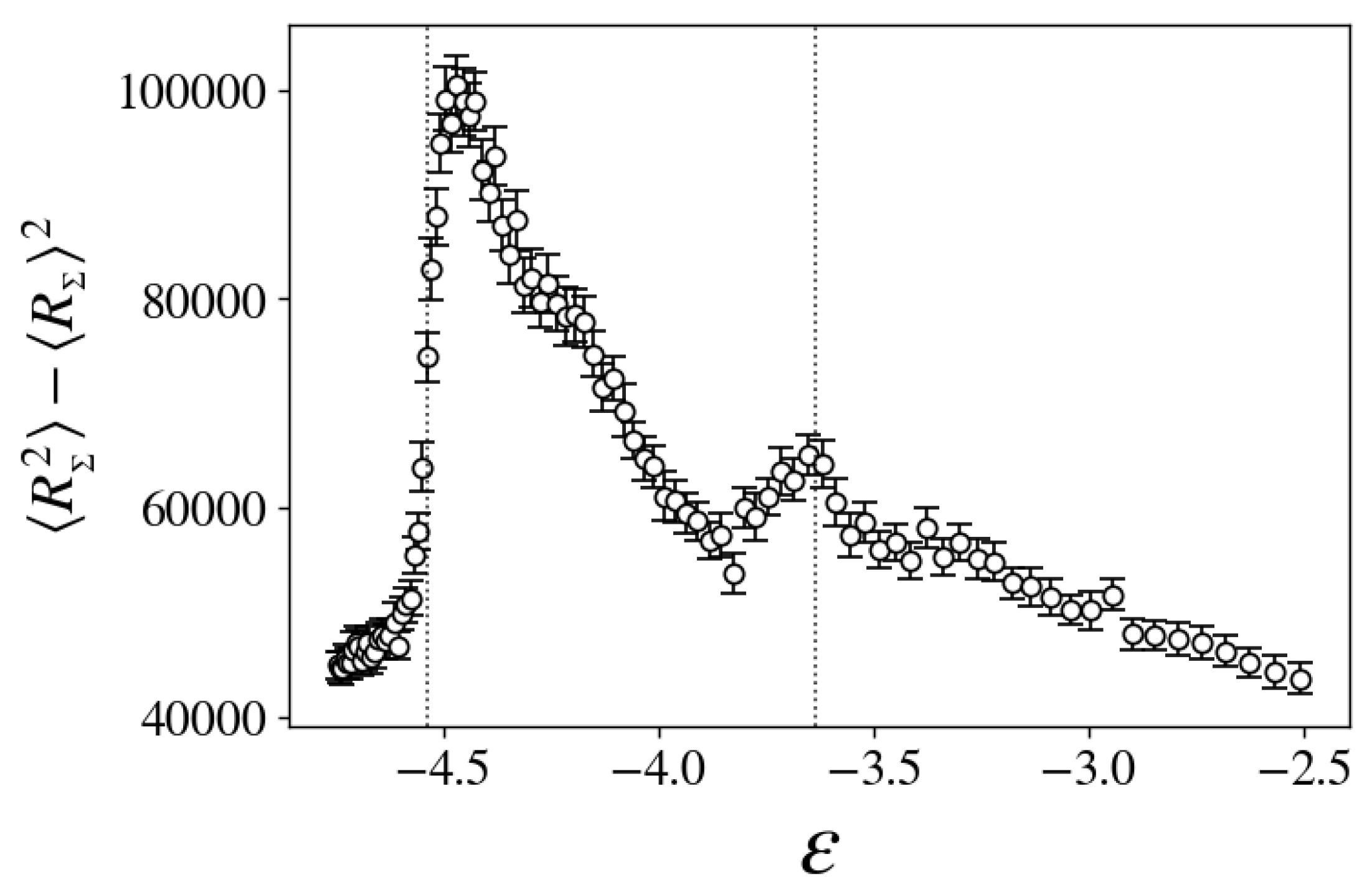
Finally, the variance of the scalar curvature, shown in Figure 9, jumps in , exhibiting a wide peak in the intermediary region, and a second, smaller peak in . As per Overholt’s theorem (6), this quantity is an upper bound to the alternate sum of the Betti numbers. These sharp changes are thus indications of major topological changes of the PLS.
All of these observations suggest that there are indeed important changes in the topology of at play in correspondence with these two critical points of . In this intermediary region, the overall shape of the manifold most probably undergo dramatic changes. These changes correspond to the rearrangement of particle configurations in pseudo-crystalline orders upon cooling.
4. Discussion
In this work, we addressed the phenomenon of glass transition using a novel approach, considering its relation with topological changes of the PLS. Using a Monte Carlo algorithm, we studied on the equilibrium properties of a glass-forming system.
Although the glass transition is often considered a fundamentally dynamical phenomenon, we gathered several indications that the system, despite having reached equilibrium, did not fully crystallize and yet exhibits clear signatures of phase transitions. This is due to the frustrated nature of the model, a Lennard-Jones binary mixture with competing interactions, that lacks a well-defined crystalline phase at the studied density.
To overcome ergodicity breaking, we employed advanced numerical techniques that allowed the system to “jump” between confining energy minima. This, combined with the absence of a crystalline phase in this frustrated system, enabled us to perform equilibrium measurements of the glass phase, based on importance sampling of the state space.
Through microcanonical analysis of the entropy derivatives, we identified two distinct transitions: a low-energy, second-order transition and a higher-energy, first-order transition. We conjecture that the first order transition is in fact a glass-liquid transition, while the second order one is a reconfiguration of the glass into different local orderings. This is supported by our finding of important changes of the radial pair distribution function and of the bond-orientational order parameters at the transitions points. These results do not correspond to what could be expected in a crystal, and are instead in agreement with recent studies [10,11] suggesting that the glass transition can be understood in terms of frustration on the way to crystallization.
Finally, in agreement with the topological theory of phase transition, we observed that several quantities that are deeply linked with the topology of the PLS exhibit inflection points and discontinuities at the transition energies. This study introduces a new approach in our understanding of the phenomenon of vitrification.
Future perspectives include the repetition of our experiment with different system sizes, to be able to perform finite-sized scaling, confirming our findings and calculating critical exponents. It would also be of interest to identify crystalline seeds in the material, and perform localized measurements of the same quantities investigated in the present work, to compute spatial correlation functions. Doing so, spatial correlation functions could be computed, which we expect to present divergent behavior around the transition energies (see [11]. Furthermore, it would reveal to which extent the topological analysis in this context is sensible to the scaling. In other words, whether the well-known degeneracy of the energy minima in the glass phase is an inherently global phenomenon, and if the system finds locally well-defined energy minima.
Author Contributions
Conceptualization, A.V., R.F. and M.P.; methodology, A.V.; software, A.V.; validation, A.V., R.F. and M.P.; formal analysis, A.V., R.F. and M.P.; investigation, A.V.; data curation, A.V.; writing—original draft preparation, A.V.; writing—review and editing, A.V., R.F. and M.P.; visualization, A.V.; supervision, R.F. and M.P. All authors have read and agreed to the published version of the manuscript.
Data Availability Statement
The raw data supporting the conclusions of this article will be made available by the authors on request.
Acknowledgments
The authors acknowledge support from the RESEARCH SUPPORT PLAN 2022 - Call for applications for funding allocation to research projects curiosity-driven (F CUR) - Project “Entanglement Protection of Qubits’Dynamics in a Cavity”– EPQDC and from INFN-Pisa. Furthermore, the authors acknowledge support from the Italian National Group of Mathematical Physics (GNFM-INdAM).
Conflicts of Interest
The authors declare no conflicts of interest.
Appendix A. Monte Carlo Methods
Simulating glass formers is a notoriously complex task, due to the large number of energy minima in the glass phase, where systems tend to get trapped. To sample the energy surface effectively, we use a Monte Carlo algorithm (MC), a common choice for equilibrium simulations. It is a class of ergodic algorithms, relying on random displacements rather than exact dynamics, allowing them to avoid getting stuck in potential wells. Unlike molecular dynamics, MC methods do not require solving equations of motion, offering significant computational speedup.
In a sound MC algorithm, provided the selection probability of a given configuration is uniform, the maximal acceptance rate satisfying detailed balance writes [26]
where and denote two distinct microstates, and p their probability weights in the chosen Gibbs ensemble statistics.
Microcanonical MC are uncommon in the literature, and less straightforward in their implementation because, in this ensemble, the system is strictly constrained to a surface of constant energy, hence evolves in a subspace of null measure in .
To address this difficulty, we use the separability of the partition function. As, at equilibrium, momenta trivially follow the Boltzmann distribution, random momentum changes at each step of the algorithm are unnecessary. Ignoring these degrees of freedom leaves the kinetic energy available as a free parameter. We use it instead as a “demon” to compensate the changes of potential energy and maintain the total energy of the system at the desired value.
The microcanonical probability density for a given microstate at energy E is given by [13,27,28]
where is the potential energy of the configuration and is the Heaviside function.
Let us now consider a transition . For any physically meaningful initial state, we must have , hence . Eq. (A1) becomes
To fully take advantage of the MC framework, we implemented moves that allow then system to escape potential wells.
First, we introduced particle swapping, first proposed in [17]. At each MC step, with a probability that we (arbitrarily) set to , one particle of each species is chosen at random, both their positions are swapped then displaced according to the usual random displacement rule; with probability , a conventional MC step is performed. Afterwards, the move is accepted according to the usual acceptance rate (A3).
We also resorted to a replica exchange (RE) algorithm, often called in the literature parallel tempering. We thereafter use the term RE, renouncing the conventional terminology which is here somehow misleading, given that the control parameter of our simulations is energy rather than temperature.
M replicas of the system are simulated in parallel, each at a different energy. Every 2000 sweeps (a sweep equates N MC steps), an attempt is made to exchanges replicas of neighboring energies.
The acceptance rate for the exchange of a replica i of energy in state with a replica of energy in state is straightforwardly deduced from detailed balance
As , its large N limit is relevant to evaluate the performance of our RE scheme , even in our relatively small system. We easily derive
which in practice were valid throughout all of our simulations.
Clearly, the overall efficiency of the RE algorithm strongly depends on the overlaps of the potential energy distributions , and therefore on the number of replicas M, and on the choice of energy array . We found that it is not enough, for a fixed M, to choose linear or exponential energy spacings. Some energies regions indeed behave as bottlenecks, through which replicas cannot diffuse efficiently enough, thus requiring finer optimization of the energy array.
We thus resorted to a simple algorithm, described in Refs. [29,30], in the context of canonical ensemble simulations, and coined in this context the energy method (which would be for us the potential method); the adaptation to the microcanonical case is straightforward. Given two fixed extremal energies and the number M of replicas we wish to simulate, it consists in finding the intermediate energies such that the exchange rate between adjacent replicas is uniform. In other words, we look convergence towards the fixed points . In principle, the closest we are to these fixed points, the more efficient is the RE algorithm.
In Refs. [29,30] (thus, in the canonical context), the average acceptance rates were computed by simply inserting the average energies into the Boltzmann weight corresponding the transition. In the microcanonical context, we cannot proceed as straightforwardly, since the acceptance rate roughly reads as (A5): simply inserting the average potential energy would result in null or much too small average acceptance rates.
To get around this issue, we simply take into account the overlap of potential energy distributions instead of the mere average, that is
Then, applying the approximation (A5) greatly accelerate the algorithm, as it avoids many exponentiation and reduces the interval on which the above integral in computed. We end up with
To estimate the distributions , we initially set the energy array following a power law, i.e. with , and run MC simulations until we obtain a reasonable energy-temperature dependence. We then computed and interpolated the average and standard deviation of as functions of E, so that we were able to roughly estimate the distributions as plain Gaussian distributions.
The integrals (A7) were finally computed numerically, using a discrete set of potential energies in the range
| Algorithm: E-range optimization through U-overlap method |
 |
Appendix B. Initial Configuration, Periodic Boundary Conditions and Cutoff
The system was simulated in a cubic box of volume .
The continuous potential (12), depends on negative powers of the interatomic distances and repulsive at short range. When some become to small, the energy thus diverges. Since our simulations were performed at high density (), totally random initial configurations typically result in very high energies, which cannot be corrected by the choice of K, since the latter is a positive quantity.
To get around this issue and have a sufficient control over the initial , we had to implement initial conditions with a high degree of symmetry. Namely, we initially arranged the particles in a cubic lattice configuration, where each particle’s first neighbors are of the other species. Then we randomly replaced particles of species 1 by particles of species 2, until we reach the desired species ratio.
To avoid undesired boundary effects, we implemented, as is it customary, periodic boundary conditions (PBC).
Remark that the PBC entails a periodic pattern in the particles’ spatial distribution. Smooth cutoffs must therefore be implemented, not only for performance purposes, but also to avoid this unwanted symmetry introduced by the PBC. Since we aim at computing quantities derived from both the gradient and the Hessian of , we accordingly needed cutoffs that is continuous up to the second order.
The non-monotonic, interspecies potential of Eq. (12) is redefined as
On the other hand, the monotonic, intra-species potentials are redefined as
where .
Following [31], we set , i.e. the distance such that . Though this condition becomes meaningless for the monotonic potentials, we also, arbitrarily, chose .
References
- Pettini, M. Geometry and Topology in Hamiltonian Dynamics and Statistical Mechanics; Vol. 33, Interdisciplinary Applied Mathematics, Springer New York: New York, NY, 2007. [Google Scholar] [CrossRef]
- Angell, C. Perspective on the Glass Transition. Journal of Physics and Chemistry of Solids 1988, 49, 863–871. [Google Scholar] [CrossRef]
- Parisi, G. The Physics of the Glass Transition. Physica A: Statistical Mechanics and its Applications 2000, 280, 115–124. [Google Scholar] [CrossRef]
- Angelani, L.; Di Leonardo, R.; Ruocco, G.; Scala, A.; Sciortino, F. Saddles in the Energy Landscape Probed by Supercooled Liquids. Physical Review Letters 2000, 85, 5356–5359. [Google Scholar] [CrossRef] [PubMed]
- Broderix, K.; Bhattacharya, K.K.; Cavagna, A.; Zippelius, A.; Giardina, I. Energy Landscape of a Lennard-Jones Liquid: Statistics of Stationary Points. Physical Review Letters 2000, 85, 5360–5363. [Google Scholar] [CrossRef] [PubMed]
- Morse, M. The Calculus of Variations in the Large, repr ed.; Number 18 in Colloquium Publications / American Mathematical Society, American Mathematical Society: Providence, R.I, 2014. [Google Scholar]
- Gori, M.; Franzosi, R.; Pettini, M. Topological Origin of Phase Transitions in the Absence of Critical Points of the Energy Landscape. Journal of Statistical Mechanics: Theory and Experiment 2018, 2018, 093204. [Google Scholar] [CrossRef]
- Di Cairano, L.; Gori, M.; Pettini, M. Topology and Phase Transitions: A First Analytical Step towards the Definition of Sufficient Conditions. Entropy 2021, 23, 1414. [Google Scholar] [CrossRef] [PubMed]
- Di Cairano, L.; Gori, M.; Pettini, G.; Pettini, M. Hamiltonian Chaos and Differential Geometry of Configuration Space–Time. Physica D: Nonlinear Phenomena 2021, 422, 132909. [Google Scholar] [CrossRef]
- Leocmach, M.; Tanaka, H. Roles of Icosahedral and Crystal-like Order in the Hard Spheres Glass Transition. Nature Communications 2012, 3, 974. [Google Scholar] [CrossRef] [PubMed]
- Tanaka, H. Bond Orientational Order in Liquids: Towards a Unified Description of Water-like Anomalies, Liquid-Liquid Transition, Glass Transition, and Crystallization: Bond Orientational Order in Liquids. The European Physical Journal E 2012, 35, 113. [Google Scholar] [CrossRef]
- Bel-Hadj-Aissa, G.; Gori, M.; Penna, V.; Pettini, G.; Franzosi, R. Geometrical Aspects in the Analysis of Microcanonical Phase-Transitions. Entropy 2020, 22, 380. [Google Scholar] [CrossRef]
- Pearson, E.M.; Halicioglu, T.; Tiller, W.A. Laplace-Transform Technique for Deriving Thermodynamic Equations from the Classical Microcanonical Ensemble. Physical Review A 1985, 32, 3030–3039. [Google Scholar] [CrossRef] [PubMed]
- Di Cairano, L.; Capelli, R.; Bel-Hadj-Aissa, G.; Pettini, M. Topological Origin of the Protein Folding Transition. Physical Review E 2022, 106, 054134. [Google Scholar] [CrossRef]
- Bel-Hadj-Aissa, G.; Gori, M.; Franzosi, R.; Pettini, M. Geometrical and Topological Study of the Kosterlitz–Thouless Phase Transition in the XY Model in Two Dimensions. Journal of Statistical Mechanics: Theory and Experiment 2021, 2021, 023206. [Google Scholar] [CrossRef]
- Coslovich, D.; Pastore, G. Dynamics and Energy Landscape in a Tetrahedral Network Glass-Former: Direct Comparison with Models of Fragile Liquids. Journal of Physics: Condensed Matter 2009, 21, 285107. [Google Scholar] [CrossRef]
- Grigera, T.S.; Parisi, G. Fast Monte Carlo Algorithm for Supercooled Soft Spheres. Physical Review E 2001, 63, 045102. [Google Scholar] [CrossRef] [PubMed]
- Pettini, G.; Gori, M.; Franzosi, R.; Clementi, C.; Pettini, M. On the Origin of Phase Transitions in the Absence of Symmetry-Breaking. Physica A: Statistical Mechanics and its Applications 2019, 516, 376–392. [Google Scholar] [CrossRef]
- Schnabel, S.; Seaton, D.T.; Landau, D.P.; Bachmann, M. Microcanonical Entropy Inflection Points: Key to Systematic Understanding of Transitions in Finite Systems. Physical Review E 2011, 84, 011127. [Google Scholar] [CrossRef] [PubMed]
- Qi, K.; Bachmann, M. Classification of Phase Transitions by Microcanonical Inflection-Point Analysis. Physical Review Letters 2018, 120, 180601. [Google Scholar] [CrossRef]
- Bachmann, M. Novel Concepts for the Systematic Statistical Analysis of Phase Transitions in Finite Systems. Journal of Physics: Conference Series 2014, 487, 012013. [Google Scholar] [CrossRef]
- Steinhardt, P.J.; Nelson, D.R.; Ronchetti, M. Bond-Orientational Order in Liquids and Glasses. Physical Review B 1983, 28, 784–805. [Google Scholar] [CrossRef]
- Errington, J.R.; Debenedetti, P.G.; Torquato, S. Quantification of Order in the Lennard-Jones System. The Journal of Chemical Physics 2003, 118, 2256–2263. [Google Scholar] [CrossRef]
- Valdes, L.C.; Affouard, F.; Descamps, M.; Habasaki, J. Mixing Effects in Glass-Forming Lennard-Jones Mixtures. The Journal of Chemical Physics 2009, 130, 154505. [Google Scholar] [CrossRef] [PubMed]
- Truskett, T.M.; Torquato, S.; Debenedetti, P.G. Towards a Quantification of Disorder in Materials: Distinguishing Equilibrium and Glassy Sphere Packings. Physical Review E 2000, 62, 993–1001. [Google Scholar] [CrossRef]
- Newman, M.E.J.; Barkema, G.T. Monte Carlo Methods in Statistical Physics; Clarendon Press ; Oxford University Press: Oxford : New York, 1999. [Google Scholar]
- Ray, J.R. Microcanonical Ensemble Monte Carlo Method. Physical Review A 1991, 44, 4061–4064. [Google Scholar] [CrossRef] [PubMed]
- Lustig, R. Microcanonical Monte Carlo Simulation of Thermodynamic Properties. The Journal of Chemical Physics 1998, 109, 8816–8828. [Google Scholar] [CrossRef]
- Hukushima, K. Domain-Wall Free Energy of Spin-Glass Models: Numerical Method and Boundary Conditions. Physical Review E 1999, 60, 3606–3613. [Google Scholar] [CrossRef] [PubMed]
- Rozada, I.; Aramon, M.; Machta, J.; Katzgraber, H.G. Effects of Setting the Temperatures in the Parallel Tempering Monte Carlo Algorithm. Physical Review E 2019, arXiv:cond-mat, physics:physics/1907.03906]100, 043311. [Google Scholar] [CrossRef]
- Holian, B.L.; Evans, D.J. Shear Viscosities Away from the Melting Line: A Comparison of Equilibrium and Nonequilibrium Molecular Dynamics. The Journal of Chemical Physics 1983, 78, 5147–5150. [Google Scholar] [CrossRef]
Figure 1.
Specific heat as a function of the energy density , in a system with . The blue squares were obtained using Eq. (14), while the red circles were obtained using Eq. (13). The dashed line is an arbitrary fit, meant to guide the eye.
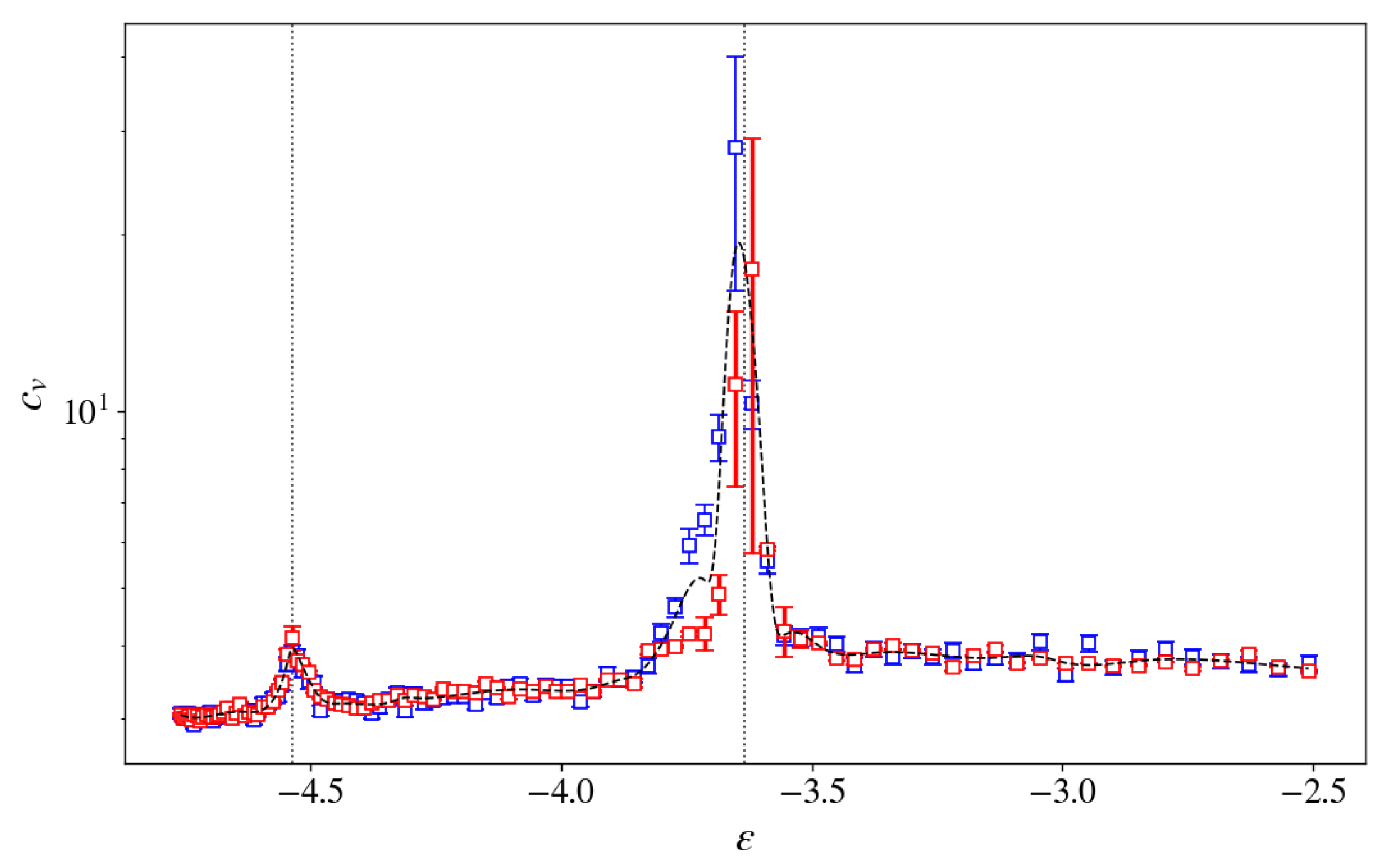
Figure 2.
Average temperature T as a function of the energy density.

Figure 3.
The first three derivatives of the entropy as functions of the energy density : (a), (b), and (c).
Figure 3.
The first three derivatives of the entropy as functions of the energy density : (a), (b), and (c).

Figure 4.
Instantaneous sample configurations projected onto a arbitrary planes, at energy density (a) , (b) and (c). Particles of species 1(2) are represented in red(blue) respectively.
Figure 4.
Instantaneous sample configurations projected onto a arbitrary planes, at energy density (a) , (b) and (c). Particles of species 1(2) are represented in red(blue) respectively.
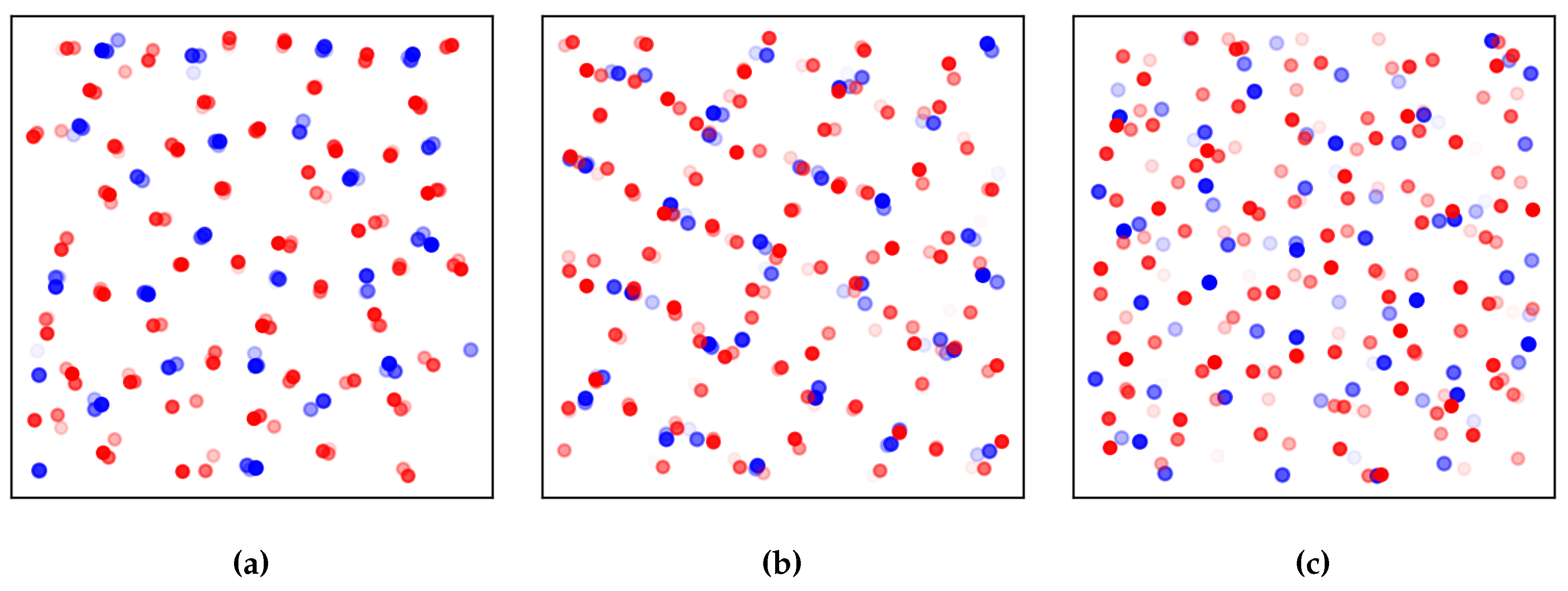
Figure 5.
Radial pair distribution function, for (a) bonds, (b) bonds and (c) bonds.
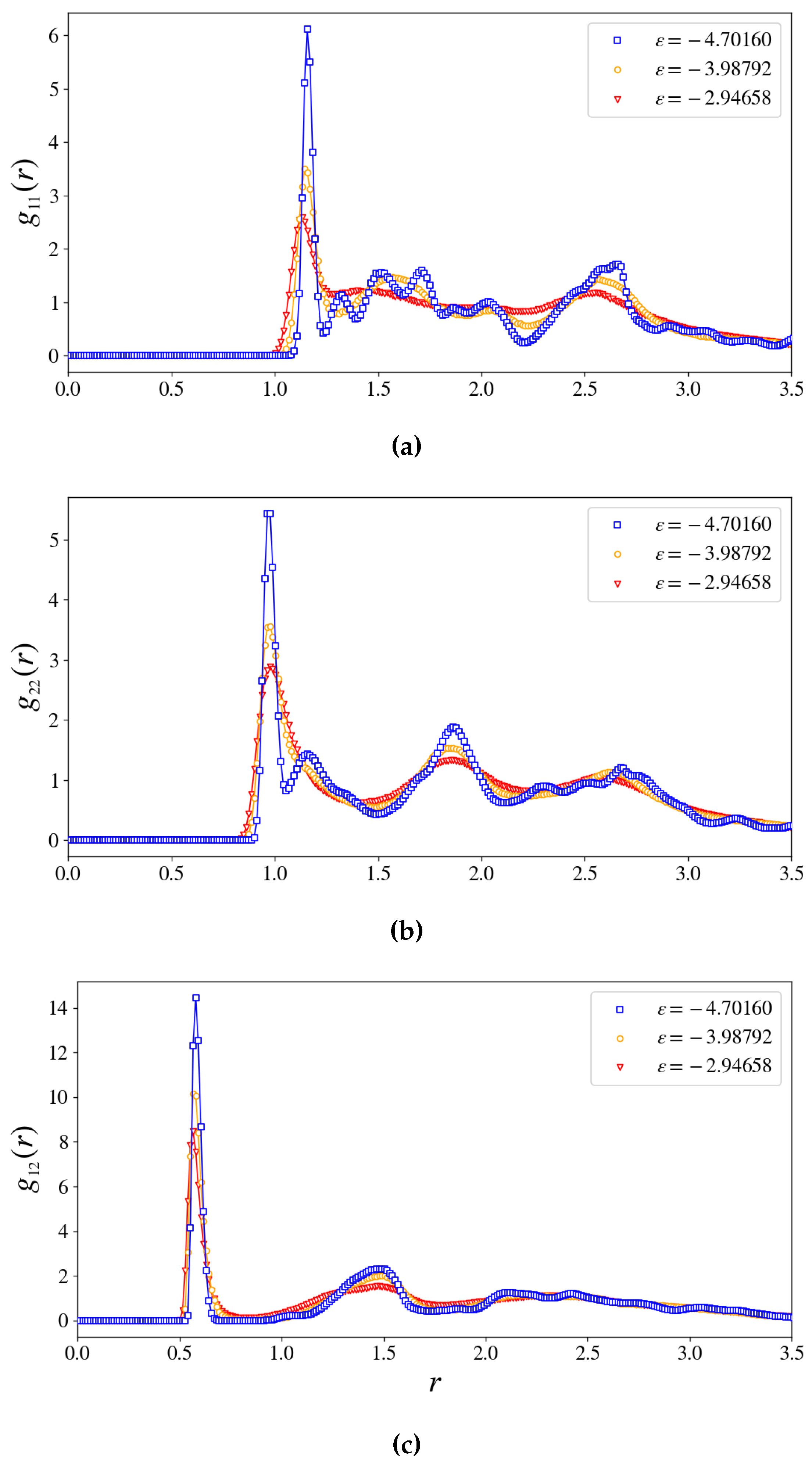
Figure 6.
Bond-orientional order parameters as a function of the energy density , (a) bonds, (b) bonds and (c) bonds. Represented are the parameters (yellow squares), (red circles), (blue triangles), (green diamonds) and (purple pentagons). The value , expected in a fully disordered system, is shown as a black line.
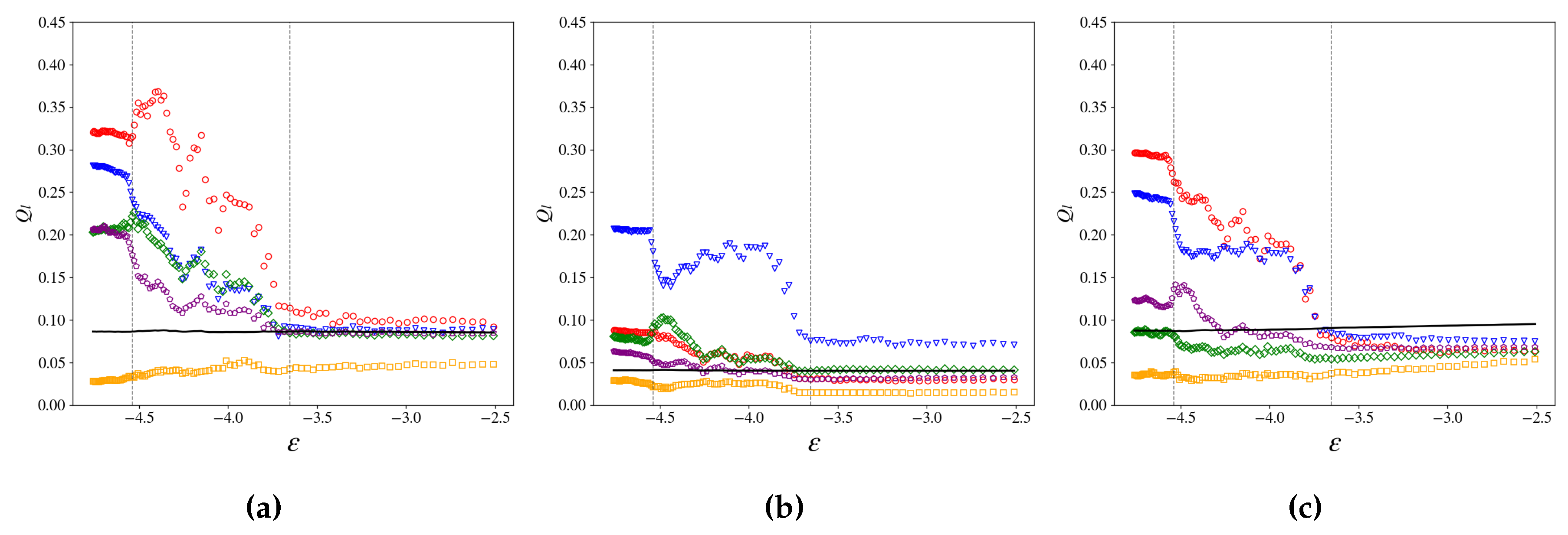
Figure 7.
Total mean curvature as a function of the energy density.
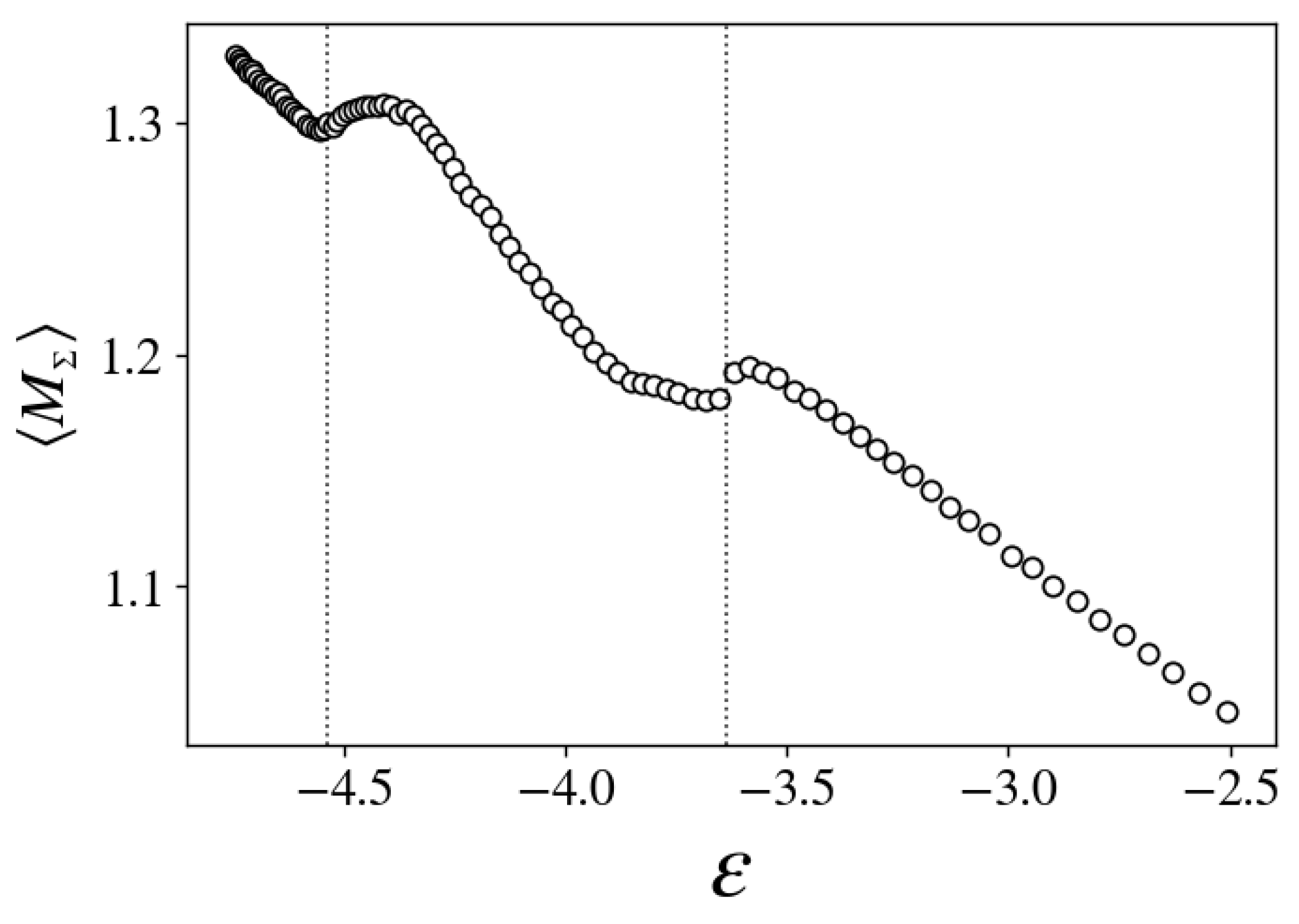
Figure 8.
Dispersion of the principal curvatures as a function of the energy density.
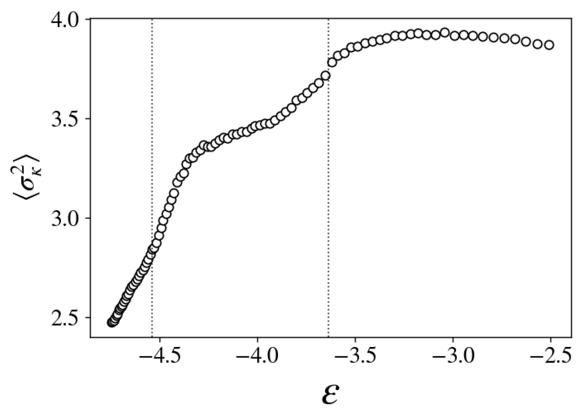
Figure 9.
Variance of the scalar curvature as a function of the energy density.
Disclaimer/Publisher’s Note: The statements, opinions and data contained in all publications are solely those of the individual author(s) and contributor(s) and not of MDPI and/or the editor(s). MDPI and/or the editor(s) disclaim responsibility for any injury to people or property resulting from any ideas, methods, instructions or products referred to in the content. |
© 2024 by the authors. Licensee MDPI, Basel, Switzerland. This article is an open access article distributed under the terms and conditions of the Creative Commons Attribution (CC BY) license (http://creativecommons.org/licenses/by/4.0/).
Copyright: This open access article is published under a Creative Commons CC BY 4.0 license, which permit the free download, distribution, and reuse, provided that the author and preprint are cited in any reuse.


