
Submitted:
03 January 2025
Posted:
06 January 2025
You are already at the latest version
Abstract
The demand for effective indoor positioning and navigation systems has surged in response to the increasing reliance on accurate location services within environments where traditional GPS is ineffective. This paper presents a comprehensive overview of the current landscape of indoor localization technologies, highlighting their applications across various industries. Despite significant advancements, challenges such as signal interference and dynamic obstacles persist, hindering the accuracy and efficiency of existing systems. To address these issues, we propose an algorithm that integrates advanced indoor mapping techniques with an iterative A* pathfinding approach. Our Algorithm utilizes Received Signal Strength Indicator (RSSI) values to ascertain user location through trilateration, while a user-friendly graphical interface allows for intuitive barrier placement and dynamic checkpoint selection. This framework not only improves navigation accuracy in complex indoor environments but also enhances operational efficiency by facilitating optimal pathfinding. Through empirical validation, our approach demonstrates a significant reduction in search times and an increase in productivity, underscoring its potential to transform indoor navigation practices. The findings contribute to the ongoing discourse on indoor positioning technologies, offering a robust solution to the challenges faced in navigating intricate indoor spaces.
Keywords:
indoor positioning
; navigation
; localization
; pathfinding
; trilateration
; indoor navigation
; RSSI
; A*
1. Introduction
In recent years, the global market for indoor positioning and navigation systems has experienced substantial growth, propelled by the increasing demand for precise location services in environments where traditional GPS signals are inadequate [1]. Industry reports indicate that the indoor positioning and navigation market was valued at over USD 8.3 billion in 2023, with projections to exceed USD 25 billion by 2030, reflecting a compound annual growth rate (CAGR) of more than 16% over the next decade [2]. This surge underscores the critical reliance on indoor location services across various sectors, including retail, healthcare, and manufacturing. Given that 80% of the global population is expected to spend up to 90% of their time indoors [3], the demand for robust and accurate navigation systems in complex indoor spaces is more pressing than ever.
Industries such as logistics and manufacturing are increasingly adopting indoor localization systems to enhance operational efficiency [4], while the retail sector leverages these technologies to elevate customer experiences through targeted location-based services [5]. Research indicates that implementing indoor navigation tools can boost productivity by up to 30% in warehouse management [6] and reduce search times by as much as 25% in expansive facilities [7]. However, despite these advantages, current indoor localization technologies encounter significant challenges related to accuracy, signal interference, and the ability to navigate dynamic environments filled with obstacles.
As our world becomes more interconnected, the demand for advanced navigation systems has surged, particularly in indoor settings where traditional Global Positioning System (GPS) signals fall short [8]. The rapid expansion of wireless networks has facilitated innovative localization techniques, utilizing technologies such as Wireless Fidelity (Wi-Fi) and Bluetooth [9]. These methods, based on trilateration and signal strength analysis, present viable solutions for tracking individuals and assets within intricate indoor environments. As urban landscapes grow increasingly complex, the necessity for effective navigation tools capable of functioning under these conditions becomes paramount.
Indoor localization systems find diverse applications, from enhancing user experiences in retail and hospitality environments to supporting autonomous robot movement in warehouses and factories [10,11]. These systems often rely on algorithms that utilize signal strength measurements for accurate positioning. The Received Signal Strength Indicator (RSSI) is particularly effective in this context, providing real-time data that reflects device proximity to access points (APs). By leveraging RSSI values, localization systems can estimate user positions and adapt dynamically to environmental changes, offering a flexible solution for indoor navigation.
Despite advancements in indoor positioning technologies, challenges persist [12]. Signal interference, arising from physical barriers and environmental noise, can significantly undermine the accuracy of RSSI-based localization [13]. Also, the presence of multiple obstacles complicates pathfinding, as traditional algorithms often struggle to navigate around barriers while maintaining optimal routes [14]. Consequently, there is an urgent need for sophisticated algorithms that can merge localization data with efficient pathfinding strategies to ensure seamless navigation through complex indoor environments.
The algorithm proposed in this paper addresses these challenges by integrating advanced indoor mapping techniques with a refined pathfinding approach. Our algorithm features a user-friendly graphical user interface (GUI) that facilitates intuitive barrier placement, creating a scalable representation of the physical environment. This model empowers users to define start and end points and select multiple checkpoints along their desired routes. Using RSSI values, the system identifies the three closest APs and applies a trilateration algorithm to accurately determine the indoor location of the user. This synthesis of user-driven environment mapping and advanced localization techniques forms a robust framework for navigating through obstacles.
To optimize the pathfinding process, we implement an iterative A* algorithm that assesses potential routes based on a cost function derived from Manhattan distance calculations. This iterative approach ensures a balance between computational efficiency and the identification of the most optimal path. By dynamically rearranging checkpoints according to proximity, the algorithm enhances traversal efficiency within the indoor environment, enabling users to navigate effectively while accommodating the constraints of their surroundings.
The proposed algorithm not only emphasizes pathfinding efficiency but also addresses the necessity of robust performance in real-world scenarios. To validate the simulation results, practical experiments were conducted using a two-wheeled bot, demonstrating the effectiveness of the optimized path generated by the algorithm. The data derived from the simulation was transferred to an Arduino microcontroller, allowing the bot to navigate through a scaled version of the simulated environment with remarkable accuracy. These experiments underscore the practical applicability of our proposed algorithm and highlight its potential to enhance navigation experiences across various indoor settings. The proposed algorithm’s main contributions are summarized as follows:
- Provides a user-friendly GUI to simulate real-world spaces, allowing for barrier placement and indoor mapping before real-world application.
- Accurately determines the user’s location using signal strengths from the three nearest APs without requiring additional hardware.
- Utilizes existing infrastructure (APs) and trilateration techniques to reduce the need for additional resources, maintaining high efficiency and low operational costs.
- Dynamically rearranges user-defined checkpoints to find the most computationally efficient path, balancing speed and accuracy.
- Reduces unnecessary nodes in the path by eliminating redundant points, improving computational efficiency and runtime without sacrificing accuracy.
- Translates optimized path data into real-world robot navigation, proving the algorithm’s applicability and effectiveness in practical indoor environments.
This paper is organized as follows: Section 2 introduces foundational concepts and essential background information for understanding the proposed algorithm’s development. Section 3 offers a comprehensive review of related work, highlighting existing approaches, methodologies, and their limitations in indoor positioning and navigation. In Section 4, we detail the proposed algorithm and its core features. Section 5 evaluates the algorithm through simulations and practical experiments. Section 6 discusses the proposed algorithm from various aspects, including its practical applications in real-world scenarios and acknowledging its limitations. Also, it outlines potential avenues for future research. Finally, Section 7 concludes the paper by summarizing its key contributions.
2. Preliminary
To build an efficient and accurate indoor localization and pathfinding system, it is essential to understand the core principles that underlie these technologies. Indoor positioning systems, particularly those based on RSSI measurements, rely on the relationship between signal attenuation and distance to estimate user locations. However, the presence of obstacles and signal interference complicates this process, necessitating advanced techniques to enhance accuracy. Once localization is achieved, the A* algorithm is widely used for pathfinding, offering an effective solution for navigating complex indoor spaces. This section delves into the foundational concepts of RSSI-based localization, trilateration, signal interference, and adaptive pathfinding, highlighting the key challenges and strategies for optimizing performance in dynamic environments.
2.1. Indoor Localization using RSSI
Indoor localization systems frequently rely on the RSSI as a primary metric for estimating the distance between wireless devices [15]. RSSI measures the strength of the signal transmitted from an AP to a receiver, with signal attenuation providing an approximate indication of distance. Given that signal strength diminishes in proportion to the square of the distance, RSSI data can be used to triangulate the receiver’s location. This process is typically conducted using trilateration, which calculates the user’s position based on distance estimates from three or more known AP locations.
However, indoor environments introduce a range of complexities that can affect the accuracy of RSSI measurements [16]. Physical barriers, such as walls and furniture, as well as environmental factors like signal reflection and absorption, create noise in the signal, often leading to imprecise localization. To overcome these challenges, techniques such as filtering (e.g., Kalman filters) or machine learning models can be employed to smooth fluctuations in signal strength and improve location estimates. The design of the localization system must carefully consider the trade-off between increasing the density of APs to enhance accuracy and managing the complexity introduced by overlapping signals, which can lead to ambiguity in the trilateration process.
2.2. Trilateration and Signal Interference
Trilateration, as the primary method of location estimation in RSSI-based systems, depends on the accuracy of the distance data derived from signal strength [17]. The success of trilateration is influenced by the spatial configuration of APs. Optimally placed APs provide distinct, non-overlapping coverage zones that improve the precision of location estimates. In contrast, suboptimal placement or dense networks can result in overlapping zones, causing interference and ambiguity in the user’s position.
Signal interference is further exacerbated by the nature of indoor environments, where signals are scattered, reflected, or absorbed by obstacles. Consequently, the effective signal range varies across different spaces, introducing inconsistencies in the RSSI readings. Advanced filtering techniques are often integrated to counteract this interference, ensuring smoother signal transitions and more accurate localization outcomes. Understanding and mitigating the effects of signal interference remains a critical challenge in the design of robust indoor positioning systems.
2.3. Pathfinding with the A* Algorithm
Once the user’s position has been accurately established, the next challenge is efficient navigation within the indoor environment. The A* algorithm is widely utilized for pathfinding due to its ability to balance exploration and efficiency [18]. It operates by calculating a cost function for each possible route, combining both the known distance traveled from the starting point and a heuristic estimate of the remaining distance to the destination. The heuristic, often based on the Manhattan distance in grid-based environments, guides the algorithm towards the most promising paths while avoiding computationally expensive detours.
The strength of A* lies in its flexibility and adaptability. In scenarios where new obstacles emerge or dynamic changes occur within the environment, A* can dynamically update its search parameters to reflect the altered landscape. This is particularly useful in indoor environments, where users may encounter shifting obstacles such as movable furniture or temporary barriers. By continuously recalculating potential routes based on real-time information, A* ensures that the navigation system remains both efficient and reliable, even under changing conditions.
2.4. Integration of Localization and Pathfinding
The fusion of RSSI-based localization and A* pathfinding represents a comprehensive approach to indoor navigation. Once trilateration provides an accurate position estimate, the A* algorithm can generate the most efficient path while considering potential obstacles and environmental constraints. The iterative nature of A*, combined with real-time updates from the localization system, allows for dynamic rerouting as the user’s position or environment changes.
Moreover, user-driven factors—such as preferred routes or checkpoints—can be seamlessly integrated into the pathfinding process, allowing for more customized navigation experiences. For example, in scenarios where users must navigate through specific checkpoints or avoid certain areas, the system can adjust paths in real time, optimizing the route based on both user preferences and environmental factors. This interplay between localization and adaptive pathfinding forms the backbone of sophisticated indoor navigation systems, ensuring both precision and flexibility in complex indoor environments.
3. Literature Review
The section provides an overview of the principles and advancements in indoor localization technologies and path-planning systems for indoor navigation that are relevant to our work.
3.1. Indoor Localization
Choosing the right indoor localization technology that has the perfect balance between accuracy, and cost of implementation has always been a challenge in developing a reliable system [19]. As the number of smart device users is increasing, it has become easier than ever to retrieve necessary information from such devices for localization [20]. Even with improvements in technology, the performance of indoor localization technology depends heavily on the parameters used for location estimation [21]. Other external factors such as indoor interference, noises, multi-path effect, and channel conditions can also impact the performance of the localization algorithm.
Some of the widely used technologies for indoor localization are Visible light communication (VLC), Computer Vision, Ultrasound, Bluetooth, ultra-wideband (UWB), and, Wi-Fi [19]. Each technology has its benefits and drawbacks. VLC has high accuracy and low power consumption but the cost of implementing the system for complete indoor coverage is very high and requires the object being localized to be in line-of-sight [22]. Computer vision-based localization processing images and video provided by cameras to locate objects. Such systems require detailed knowledge of the indoor environment and generally have a high computational cost due to the processing of large quantities of data [23,24]. Ultrasound technology has high accuracy and is resistant to multipath effect but the cost of implementation is high, energy efficiency is low and it is highly susceptible to environmental noise[25]. In [26], the authors implemented pulse compression using a modified binary phase shift keying (BPSK) demodulator at the receiver end to improve energy efficiency and reduce impact due to environmental noise but the localization accuracy decreased due to the additional computation. Bluetooth technology can be used for localization due to the availability of such technology and its low power consumption but it has a higher cost of implementation and is less accurate compared to the other methods due to its limited range and fluctuations in signal strength [27]. UWB has very high localization accuracy and low latency but it has very limited coverage, high computational cost, expensive to cover a large area with this technology and the accuracy falters if there are any obstacles between the UWB anchors and tag [28]. Poulose et al. [29] proposed a deep learning approach where UWB data was used by long short-term memory (LSTM) networks to estimate and predict the user position and improve localization accuracy. The results show that the implementation of the LSTM network improves the localization accuracy compared to the conventional methods but there is no mention of the increase of computational cost. The increase in computational cost will have a large impact on the viability of such models for various scenarios that require real-time or large-scale localization.
Wi-Fi is one of the most widely used wireless technologies for indoor localization due to its availability, no line of sight requirements, low implementation cost, no additional hardware or software requirements, and reasonable accuracy [19,30,31]. The Wi-Fi devices which are usually called access points (APs) are connected to the user’s devices and these signals can be analyzed using its parameters to locate the device [32]. Internal characteristics related to Wi-Fi use signal parameters such as time-of-flight (ToF), angle of attack (AoA), channel state information (CSI), and RSSI for indoor localization [19]. The algorithms can be used individually or can also be combined depending on the requirements of the system and the available resources. ToF-based localization uses the signal propagation delay to estimate the distance between the AP and the device and locate the device using trilateration. In [33], the authors described the various stages to simulate a ToF-based indoor localization system. Authors in [34] combine ToF with RSSI to improve localization accuracy and reduce the localization measuring time. AoA estimates the angle at which the signal arrives at the device from different APs. The advantage of using this parameter is that the location can be estimated with two APs in a 2D environment [19]. However, as the distance between the APs and the device becomes larger, the error in location estimation also increases [35]. Kotaru et al [36] used CSI and RSSI to implement a super-resolution algorithm to improve the AoA and ToF calculations for indoor localization such that the multipath effect is minimized. CSI shows the best performance in terms of localization accuracy and latency as it is resistant to the multipath effect but one major issue is that many of them are not widely available on standard router network interface card (NIC) [37].
Due to low computational complexity and no additional cost of implementation, RSSI becomes the choice of localization parameter. Wi-Fi technology utilizing RSSI-based trilateration algorithm provides an accurate estimate of the indoor position in real-time [38]. This method uses the log-distance path loss model for distance estimation. However, the accuracy decreases due to the multipath effect and environmental noise. In [39], the authors used the non-linear iterative least squares method for estimating the location of APs and also the parameters of the path loss model to improve the localization accuracy of devices. Yang et al. [40] propose data preprocessing techniques using Gaussian filters to preprocess the RSSI data, the transmitted power and path loss exponent are measured using least-squares curve fitting during distance calculation, and Bayesian filters are used to further reduce errors in distance calculations. Both theoretical and practical experiments were conducted on both LOS and NLOS scenarios and the results show that the proposed system improves the accuracy of the RSSI-based localization. However, due to the additional computational requirements of both [39] and [40], the localization delay increases, and further experiments are required to analyze the performance of the models on large indoor spaces.
3.2. Path Planning
Path planning algorithm intends to identify the most efficient route from one place to another that minimizes travel distance and time while bypassing obstacles and environmental restrictions [41]. Path planning within indoor settings is a greater test as the transversal paths are restricted and the nature of the obstacle fluctuates. Relying on the structure of the indoor settings, path planning algorithms are classified as either static path planning or dynamic path planning frameworks.
Static path planning presumes that the layout and obstacles remain unaltered throughout navigation. The algorithms applied for static path planning determine the optimal route through the environment assuming the layout does not shift over time. Therefore, the pathway generated by a static path planning algorithm represents the global solution for the specified layout [42]. However, static path-planning algorithms fail when the layout or barriers modify or shift over time. The formulation of dynamic path-planning algorithms conquers these challenges and adapts the route dynamically in real time by analyzing the alterations to the environment. The path generated by dynamic path-planning algorithms is the locally preferred result as the route given was the finest corresponding to the structure of the outline at points in time. Dynamic path planning algorithms provide a superior approximation of the ideal route as they align strictly with real-world scenarios where the elements in the environment are not consistently static [43].
Static path planning systems can use sampling-based, graph-based, heuristic, or artificial intelligence (AI) algorithms to find the optimal path [44]. These algorithms represent the indoor environment as a graph where each available position for movement is called a node. The objective of the algorithm is to move from the start node to the end node while transversing through the fewest nodes possible. Some of the most popular static path planning algorithms are the Dijkstra Algorithm, A* Algorithm, Particle Swarm Optimization (PSO), Ant-colony Optimization (ACO) Algorithm, and many more [41]. Dijkstra Algorithm uses a greedy approach to find the shortest path to the goal without considering the viability of the path citepgunawan2019implementation. The path provided only takes the shortest path from the current position to the next position without considering the complexities of the environment or estimating the distance to the target node. To overcome this, the A* algorithm is used which is a heuristic search algorithm that combines the Dijkstra Algorithm with the Breadth First Search (BFS) algorithm [45]. Yu et al. [46] combined ACO with the A* algorithm where ACO determines the ordering of the targets and the A* algorithm is used to transverse through the nodes individually in an environment with dense obstacles for autonomous underwater vehicle (AUV). The authors use representative-based estimation (RBE) to estimate a cost graph that can be used by ACO to determine the traveling order of the targets. The proposed system increases the computational complexity and it will cause significant delays in determining the most optimum path for large spaces with dense obstacles. Huang et al. [47] combined PSO with the A* algorithm to overcome the individual weaknesses of each algorithm such as low path accuracy and the existence of redundant nodes of the A* algorithm and reduction in path accuracy for too many objects in the large environment of PSO. The proposed system performed better than the individual algorithms but the model was evaluated theoretically on a small space. Further analysis of the performance of the model is needed for large complex spaces as the additional computation and deletion of transition nodes might decrease the path accuracy.
The path-planning algorithm can also be chosen depending on the nature of the indoor environment or the objective of navigation [48]. Algorithms such as crowd-aware fastest path query (CAFPQ) or r least crowded path query (LCPQ) find the optimized path towards the target point based on the number of both static and dynamic objects present in indoor environments [49]. Such systems mainly rely on accurately mimicking the random movement of crowds in indoor spaces and do not perform well in scenarios where the flow of crowd cannot be captured properly.
For dynamic path planning, the rapidly exploring random tree (RRT) algorithm is one of the most popular algorithms. The algorithms can find an optimized path quickly for environments with a high percentage of obstacles and high-dimensional (multi-floor) spaces [50]. Other researchers have modified the RRT algorithm to improve its path-planning performance. A heuristic RRT algorithm has been proposed by [51] that can find the optimal path through an indoor environment without modeling the environment. Bruce and Velso [52] proposed an improved RRT algorithm that uses a probabilistic RRT approach to determine the nodes to transverse through from a list of random nodes that contains nodes from previous runs of the algorithm. When the subject of path planning for people in indoor spaces is considered, static path planning is implemented in most cases as the individuals can avoid obstacles just by moving around them and large indoor spaces do not have large obstructions moving around.
3.3. Indoor Navigation Systems
Indoor navigation systems address the challenges of accurate positioning and routing in enclosed spaces while also leveraging path planning algorithms to ensure efficient and reliable path planning [53]. Suryaprakash et al. [53] implement such a system for mobile robots by using a vision-based approach to map the indoor space using cameras, utilizing sensors such as accelerometer, gyroscope, and ultrasonic sensors to estimate the robot’s position and orientation concerning its initial position and finally employs probabilistic roadmap (PRM) algorithm to find the best path to goal. Other systems such as Kantawong [54] also use vision-based approaches to find Quick Response (QR) codes to determine its position in a known floor plan for static path planning or use RFID traffic cones and exit signs placed inside the indoor environment to localize itself for dynamic path planning. Zou and Xie [55] use UWB-based trilateration systems for indoor localization and then find the most optimized path for navigation using the A* algorithm and dynamic window approach (DWA) algorithm. Wang et al. [56] use a similar approach as [55] for path planning but it uses simultaneous localization and mapping (SLAM) for mapping the area and localizing the robot. Although these systems show promising results, further analysis is required regarding the computational cost and indoor localization implementation cost. The systems also have a high indoor mapping time and path planning algorithm execution time which indicates that such systems have room for further optimization to make them viable for real-world application.
Multi-target indoor navigation systems are an extension of traditional indoor navigation systems where a user or object can be efficiently guided through multiple target positions in a complex indoor environment. One crucial area of application of multi-target indoor navigation systems is search and rescue (SAR) operations. Dong et al. [57] considered situations for coal mine disasters where the A* algorithm was implemented to get the initial path through the coal mine and afterward local multiobjective evolutionary algorithm was implemented to further optimize the path. Other SAR operation systems tackle multi-story building navigation [58] to locate and rescue multiple targets by converting the multi-story indoor environment into a graph. However, such systems have only been tested in simulations and lack practical experimental analysis. Due to the challenging indoor scenarios for SAR operations, such systems do not try to tackle the issue of indoor localization in emergencies but rather utilize prior knowledge of the indoor space for navigation. Systems can also be designed in such a way that the efficiency of the path planning algorithm increases as the number of target nodes increases [59]. However, all of the systems mentioned do not provide the user the ability to dynamically map the indoor environment and lack information regarding the accuracy of indoor localization.
4. Proposed Algorithm
In this section, we will describe in detail the proposed algorithm, the algorithm being used, and the key features of our algorithm.
4.1. Algorithm Overview
The proposed algorithm integrates multiple features aimed at optimizing pathfinding in a simulated environment that mirrors a scaled version of a physical space. Users can customize this environment via a barrier GUI, allowing for precise placement of walls and obstacles. Once the environment is established, the user’s position is determined through RSSI data, utilizing the three nearest APs. To ascertain the user’s indoor location, a trilateration algorithm processes this information, ensuring accurate positioning at key points within the environment.
Following this, the user specifies a starting point, an endpoint, and any desired checkpoints. These coordinates are seamlessly translated into the simulation environment. An iterative A* algorithm then rearranges the checkpoints to identify the path with the least computational cost while efficiently navigating through all checkpoints to reach the destination. This approach strikes a balance between computational efficiency and optimal pathfinding.
The heuristic value of each iteration of the A* algorithm is based on the distance between a set of two points (,) and (, ) that is found using Manhattan distance (), Equation (1).
Once the optimal path is determined, additional node reduction techniques are applied to minimize the number of nodes traversed. The algorithm tracks key performance metrics, including total and average runtime, the number of steps from origin to destination, and overall memory usage. Finally, the optimized path data is transmitted to the microcontroller of a robot for real-world implementation. The complete flowchart of the proposed algorithm is illustrated in Figure 1.
4.2. Core Features
This section outlines the core features of the proposed algorithm. Subsequently, Subsection 4.3 will compare these features with the related works presented in Section 3.
4.2.1. Adjustable
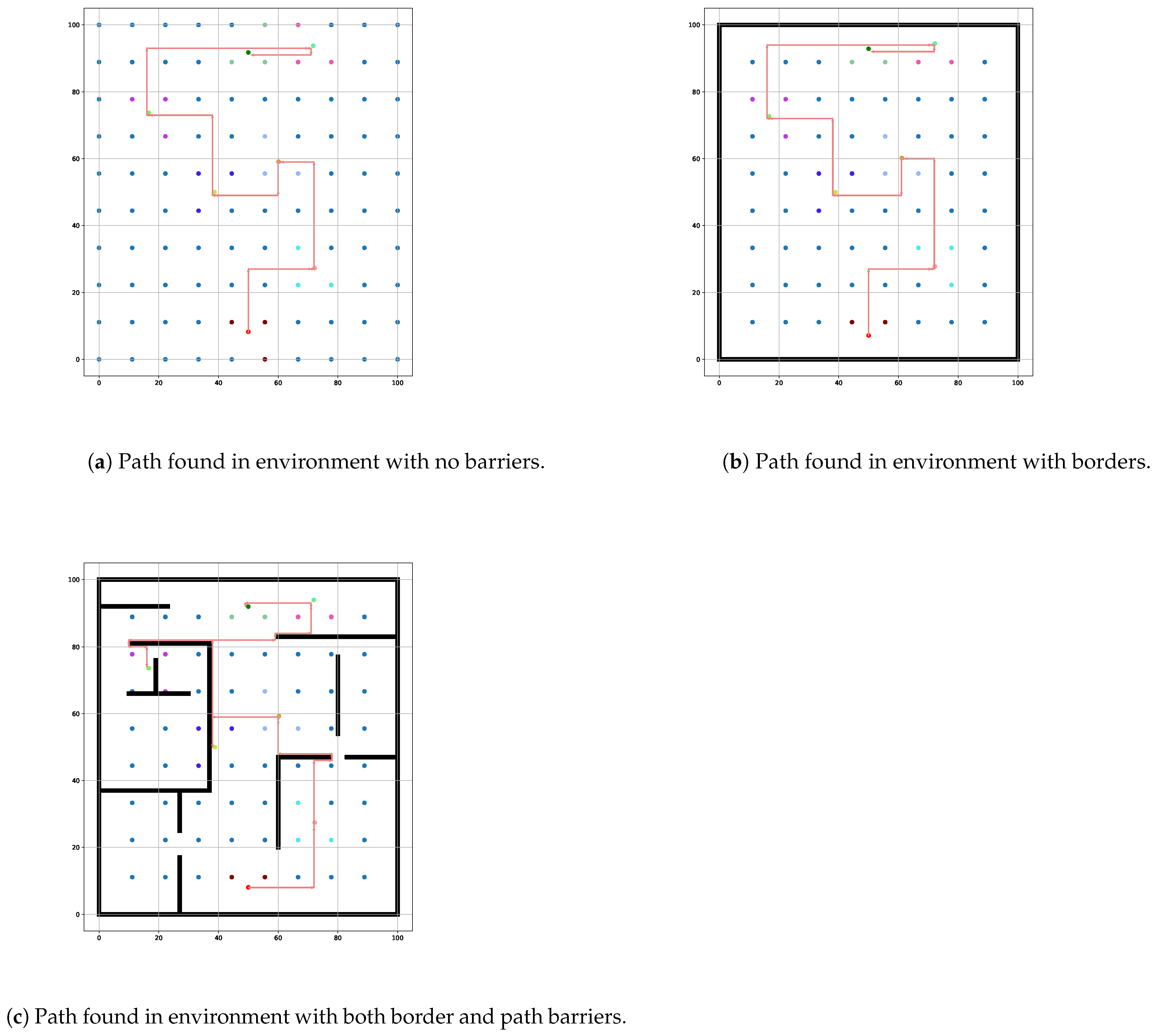
The proposed system is initiated by mapping the physical indoor environment to the simulation grid. Barriers are allocated in the simulation grid that are considered obstacles in the environment and the path planning algorithm needs to work around those obstacles to find the best path. To make the barrier placement dynamic and adjustable, a GUI was implemented. The users can click on the grids to place the barriers according to the indoor environment they want to simulate. The GUI for the barrier placement also ensures that the number of barriers or size of the barriers does not exceed the grid size. The GUI assigns coordinates to the selected grids in the () plane that will be used later when determining the best path. The Figure 2 shows the different simulation environments created using the GUI- Figure 2(a) is the initial simulation environment with no border or path barriers, Figure 2(b) is the environment with only border barriers and Figure 2(c) is the environment with both border and path barriers.
4.2.2. Traceability
To trace the user and the checkpoints indoors, the RSSI data found from the APs is used. The RSSI values range between dB, and the higher the value, the closer the object is to the AP. It is assumed that the user and the checkpoints have a device connected to the Wi-Fi network which helps determine the RSSI value. The 3 nearest APs to the user or the checkpoints are determined based on the RSSI values. The system in [60] is used to find the RSSI values and also the estimated indoor position based on the 3 nearest APs using the trilateration algorithm. The RSSI value depends on the transmitted power which is given by:
where, is the difference between transmitted power and received power, is the path loss in dB, is the path loss exponent, d is the Euclidean distance between the object and the AP and is the reference distance. The value of in buildings with obstacles ranges between and for this, the value of gamma selected is 3. The value of is negligible and hence set to 0 while the value of is set to . To find the RSSI value using , we use
where, is the loss due to signal interference, is the loss due to the multipath effect and, is the loss due to signal attenuation. The values of interference, multipath, and attenuation are in the range . The RSSI values of all APs are determined according to the distance from the user or the object and the values are sorted afterwards. The 3 APs with the highest RSSI values are chosen and then the estimated distance of the object from the chosen RSSI are used to find their coordinates for the indoor space using trilateration. The equation used in trilateration for i-th AP which is given by and the object coordinate with distances from to C, is given as:
for , where () are the coordinates of the AP closest to the object which is used as a reference, and is the distance from the object to the reference AP. To solve the system and derive the coordinates of , we model it as a system of linear equations:
where, matrix A and vector b are found using the equations (4), (5) and (6). Now we solve the system using the least square method using
Using equation (8), the coordinates for all the checkpoints and the user are derived which will be used in the A* algorithm.
4.2.3. Waypointing
The algorithm for the proposed system is designed such that the user can transverse through multiple checkpoints before reaching the goal. The indoor location of the checkpoints would also be determined using the RSSI-based trilateration algorithm. The path planning algorithm would sort the checkpoints according to the distance from the current user location. After the user moves from the start position to the first checkpoint, the checkpoints get sorted again and the process repeats till the user reaches the goal. This ensures that the checkpoints are sorted according to the direction in which the user moves and the algorithm can find the global best path to the goal. For the simulation environment, the crucial points and the APs are visualized using different colors as described in Figure 3.
For the proposed system, environments with c checkpoints have been investigated where the value of c is between . The environment with the start point, end point, and all the checkpoints along with the 3 nearest APs for each critical point is shown for all the environments in Figure 4. The impact of having only borders compared to the no border simulation environment will be on the algorithm run time and the memory usage which will be explained further in Section 5.
4.2.4. Navigational
After the coordinates of the barriers, the user, and the checkpoints are determined using trilateration, the iterative A* algorithm is used to find the best route for the user that navigates through all the checkpoints to reach the goal. Initially, it is assumed that each () coordinates on the grid which are referred to as nodes have a value of ∞. The calculated indoor location of the user is defined as the starting point. The A* algorithm calculates the cost of moving from one point to another based on
where, n is the current node with coordinates (), is the cost to reach node n from the starting point, is the heuristic estimate of the cost to reach the desired checkpoint, and is the total cost of moving to the current node from the previous node. The costs are calculated using equation (1).
At the starting point, the value of is 0 and the value of is based on . The algorithm then calculates the cost of moving to the 4 neighboring nodes of the current position. The previously set values of ∞ for each node get replaced by the actual cost of moving to the node which is given by equation (9). The algorithm ensures that it moves to the neighbor node with the lowest cost and the neighbor node becomes the current node. Only the 4 neighboring nodes in straight directions are considered as we are using Manhattan distance as the cost function.
For the first iteration of the algorithm, the start point is the initial location of the user and the checkpoints are considered as the goal. The algorithm iterates through all the checkpoints and determines the closest checkpoint based on the number of steps required to reach it. The checkpoint with the lowest number of steps from the start point is found and the algorithm makes it the new starting point and removes it from the list of checkpoints while also saving the path taken. The process is repeated till the last checkpoint becomes the starting point and then the algorithm determines the path to goal. The total number of iterations for the proposed system is defined by
where, k is the number of checkpoints excluding the start point and the goal. If there is no clear path to the checkpoints or the goal, the algorithm cannot determine the best path and hence requires the user to input other checkpoints or goals to find the best path. The path given by the iterative A* algorithm starts from the start point, passes through all the checkpoints, and finally reaches the endpoint. The path provided by the proposed algorithm for 5 checkpoints for the 3 different environments are shown by Figure 5.
Analysis of the paths found show that there is no difference in path for both the environments with no barriers and the environment with border barriers which can be seen in Figure 5(a) and Figure 5(b). The environment with path border takes a different route as the routes shown previously have obstructions. The route found for the simulation environment of Figure 2(c) is shown in Figure 5(c). The path found is longer as it needs to avoid the path barriers but it will be the best path towards the goal for the given indoor arrangement.
4.2.5. Optimization
The iterative A* algorithm finds the best path but must travel through all the nodes in the path. This increases the memory usage, path travel time, power required to transverse through the path, and computational cost. To reduce the number of nodes in the path, a node reduction technique is implemented. As Manhattan distance is used as the cost function, the paths determined will only be straight. The algorithm used for node reduction is described in Algorithm 1.
| Algorithm 1:Path Optimization via Redundant Node Removal |
|
where, is the complete path generated by iterative A* algorithm that consists of () coordinates of node n. As the path provided is straight lines, checking the gradient would not yield results in cases where the path is moving only in the x-direction. To overcome this issue, the values are checked separately. The algorithm compares difference in x and y coordinates of node n with the previous node and next node . also, the algorithm checks if the current node is one of the checkpoints or not. If the current node is between a straight line of nodes and is not a checkpoint, node n gets deleted from the variable. The path derived after node optimization is shown in Figure 16 where the algorithm only keeps only the crucial and the turning path nodes for navigating through the environment.
Figure 6.
The optimized path given by the iterative A* algorithm in the different simulation environments
Figure 6.
The optimized path given by the iterative A* algorithm in the different simulation environments
4.3. Qualitative Comparison
In this section, we present a qualitative comparison between the proposed algorithm and other approaches discussed in Section 3. The comparison focuses on the following core features: adjustability, traceability, navigational, and optimization in indoor navigation systems. Table 1 presents the results, with each feature marked by a ✓ to indicate support or a ✗ to indicate its absence. This analysis offers a concise view of the strengths and limitations of each method, providing a clear understanding of how the proposed algorithm compares to existing alternatives.
Most of the research reviewed in Section 3 have been categorized according to the features they offer in Table 1. Studies conducted in [23,25,26,27,29,33,34,35,36,37,38,39,40] only work with indoor localization technology to improve its accuracy or reduce the computational complexity while [42] only finds the path from start to the goal. Other studies such as [45,47,51,52] implement a path planning algorithm and then post-processes the path to improve the path efficiency. Research conducted in [46,57,58] only focuses on multi-target path planning whereas [48,49,53,54,55] combines both localization and path planning for indoor navigation but does not consider multiple target points. The proposed systems in [56] and [59] combine an accurate indoor localization algorithm with an efficient path planning algorithm. However, [56] can dynamically map the environment using SLAM but does not consider multiple target points whereas [59] can include multiple target points during navigation but is based on a given indoor environment and cannot make changes to it. Our proposed system includes all the features to provide the user with a comprehensive multi-target indoor navigation system that is also applicable to real-world scenarios.
5. Evaluation
In this section, we evaluate the proposed algorithm using both simulations and practical experiments. We detail the experimental setup and present the results of both approaches for the indoor path planning model. Two algorithms were tested: the Basic A* algorithm and the proposed Iterative A* algorithm.
5.1. Simulation Evaluation
This section details the comprehensive simulation evaluation performed to assess the performance of the Basic A * and Iterative A * algorithms under various environmental conditions.
5.1.1. Simulation Setup
The simulation experiments were meticulously conducted to evaluate the performance of the Basic A* and Iterative A* algorithms under various environmental conditions. The setup is as follows:
- Hardware Configuration: Experiments were executed on a Windows 10 laptop equipped with an Intel Core i7-8750H processor and 16 GB of RAM.
-
Simulation Environment: A 100 × 100 indoor grid was used to simulate different conditions. Three distinct scenarios were investigated:
- Environment 1: No obstacles or borders, serving as a baseline for performance evaluation.
- Environment 2: An environment featuring boundaries, hypothesized to influence the total and average execution times without affecting the algorithm’s path.
- Environment 3: This scenario included both borders and obstacles, aiming to assess the algorithms’ performance in more complex navigation situations.
- Evaluation Metrics: The algorithms were evaluated based on the number of different checkpoints that needed to be visited excluding the start and end nodes. The performance evaluation was done based on the average algorithm execution time, memory usage, total path length, number of turns taken, and the number of nodes after reduction.
5.1.2. Indoor Localization Simulation Result
RSSI-based trilateration algorithm was implemented to locate the start point, endpoint, and checkpoints indoors. Initially, the 3 closest APs to each of the key points were determined based on their RSSI values, and the distance from the nearest APs was determined using the path loss distance model. Finally, the trilateration algorithm was implemented to estimate the coordinates of the key points. The actual coordinates of the key points were kept constant throughout the simulation. Table 2 shows the actual coordinates of the key points, the estimated coordinates of the key points in all the simulated environments, and the error of estimation which is calculated using Equation 11.
It can be seen from Table 2 that the setup of the environment has minimal impact on the performance of the indoor localization algorithm. The approximated error in the position calculation ranges between 0.71% and 7.08%, with the average errors being 3.09% for Environment 1, 4.01% for Environment 2, and 3.19% for Environment 3 which highlights the accuracy and consistency of the localization algorithm used. The results prove that RSSI-based trilateration is not only accurate for indoor localization but also remains the most cost-effective method in terms of implementation and computational overhead.
5.1.3. Path Planning Simulation Result
The optimized paths generated by the Basic A* algorithm for the different checkpoints are shown in Figure 7 for environment 1, Figure 8 for environment 2, and Figure 9 for environment 3 while the path given by Iterative A* is shown in Figure 10 for environment 1, Figure 11 for environment 2, and Figure 12 for environment 3. The paths provided by both algorithms show that they follow nearly identical paths when the number of checkpoints is low (less than 2). This is due to the best path through the checkpoints towards the goal remaining relatively straightforward and the limited number of checkpoints allows for a direct traversal without significant deviation. However, as the number of checkpoints increases, the Iterative A* algorithm performs much better and can sort the checkpoints better for transversing while minimizing unnecessary detours. This path optimization capability of the Iterative A* algorithm is evident in Environment 3 where the presence of obstacles introduces additional complexity. The Basic A* algorithm has a more rigid approach where it only moves through the checkpoint sequentially. This approach can work well in simple scenarios but as the obstacles and number of checkpoints increase, the simple approach becomes inefficient.
Figure 7.
Optimized paths derived by the Basic A* algorithm for 0–5 checkpoints in Environment 1.
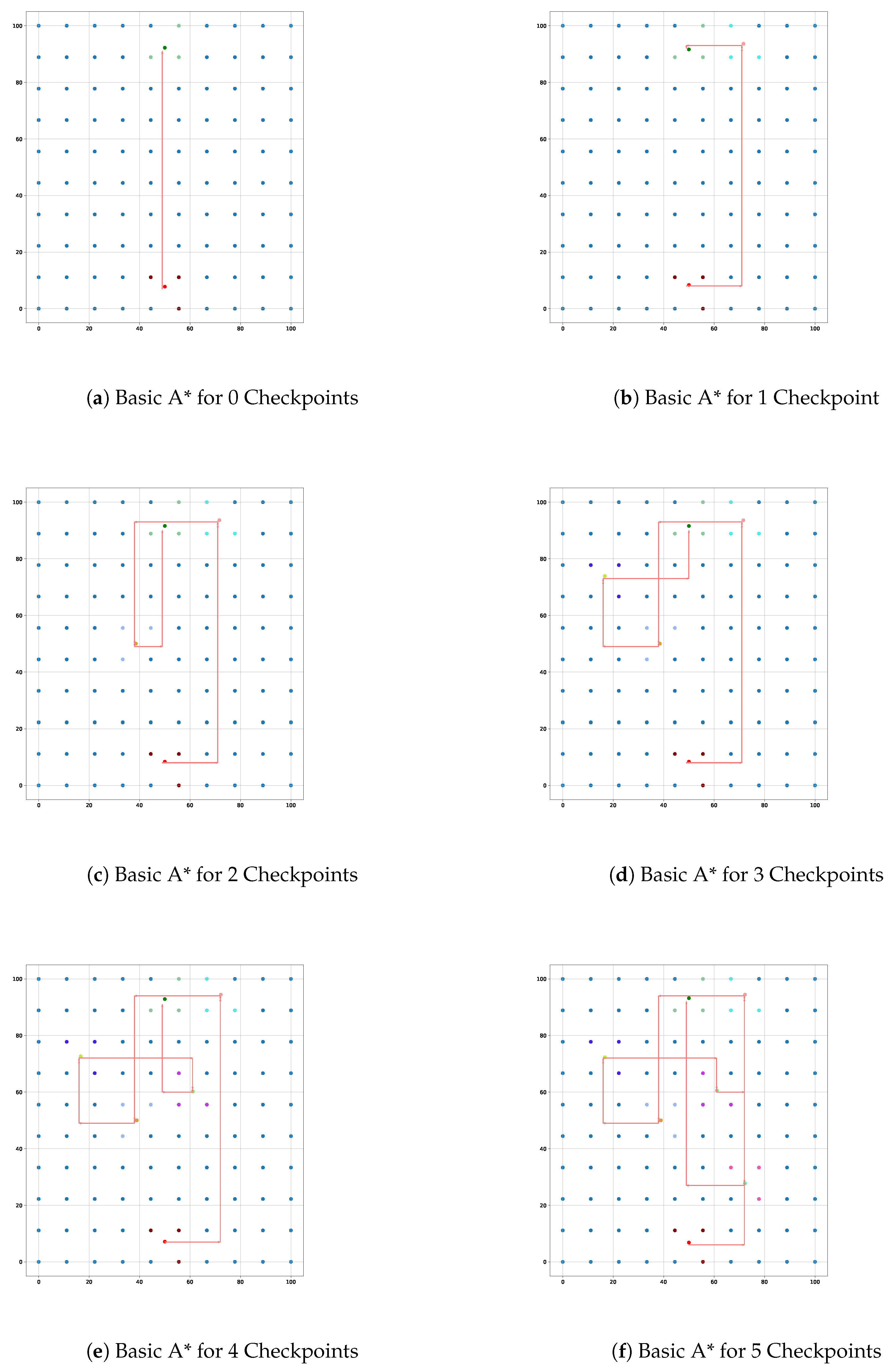
Figure 8.
Optimized paths derived by the Basic A* algorithm for 0–5 checkpoints in Environment 2.
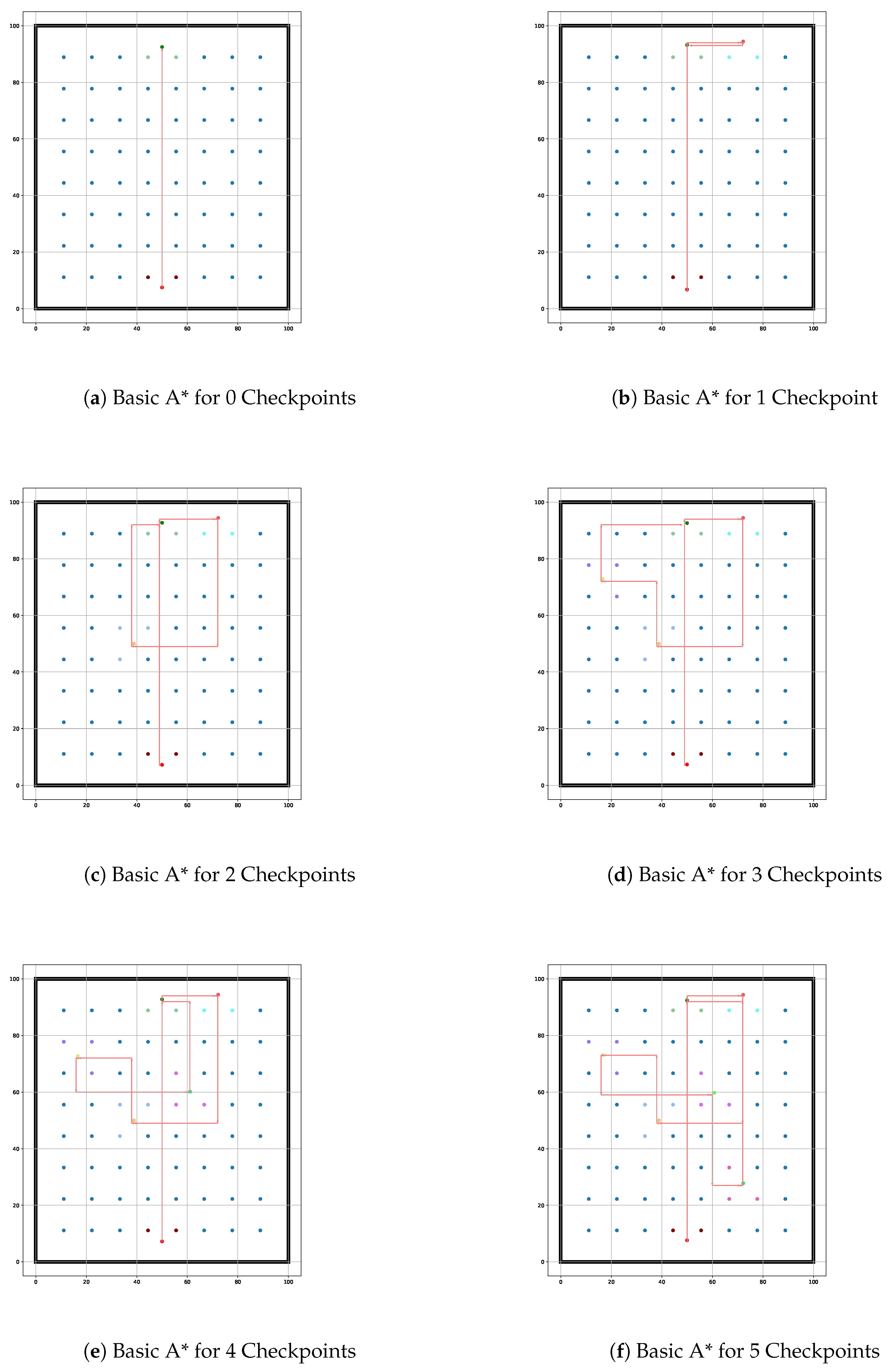
Figure 9.
Optimized paths derived by the Basic A* algorithm for 0–5 checkpoints in Environment 3.
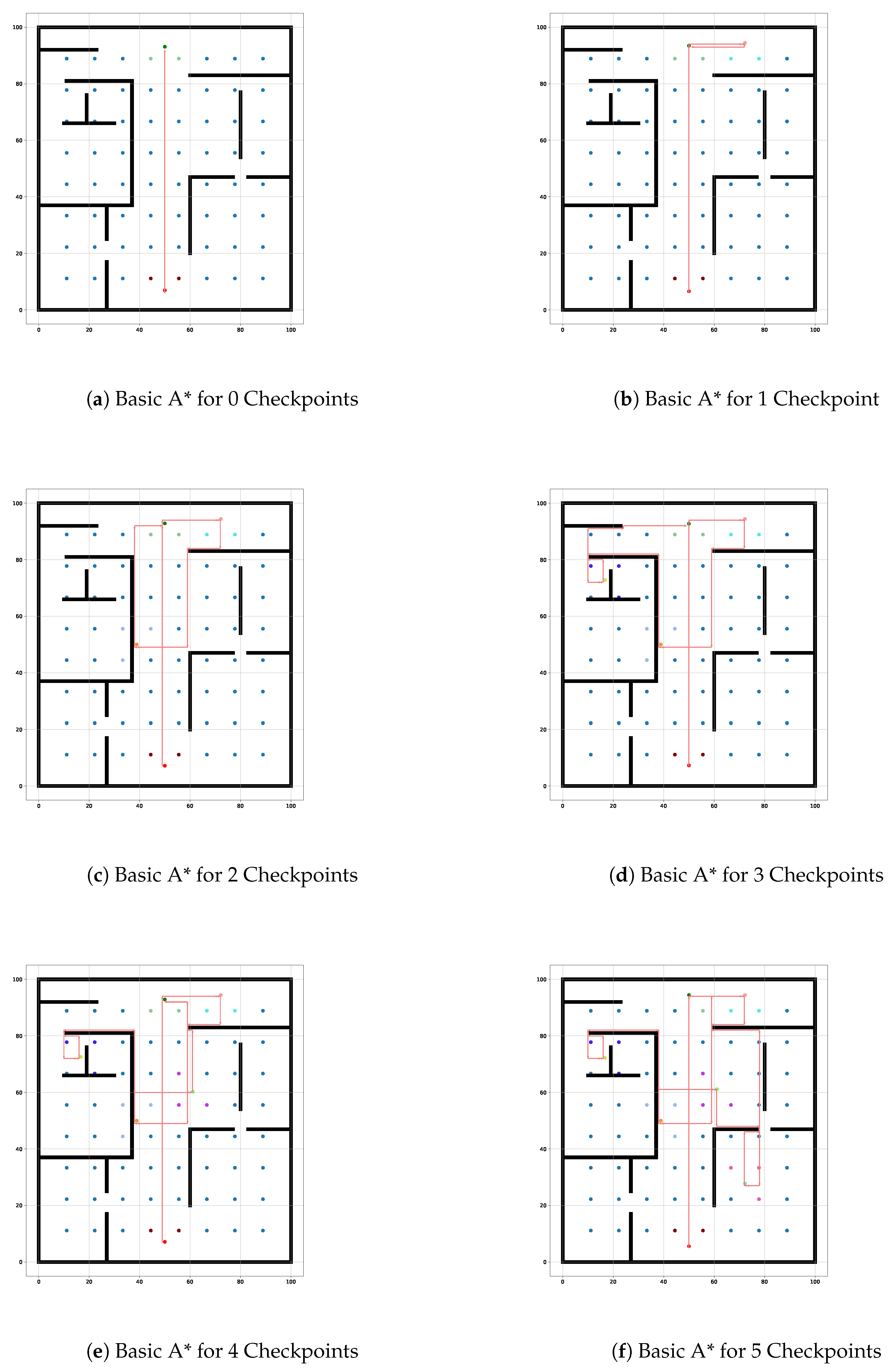
Figure 10.
Optimized paths derived by the Iterative A* algorithm for 0–5 checkpoints in Environment 1.
Figure 10.
Optimized paths derived by the Iterative A* algorithm for 0–5 checkpoints in Environment 1.
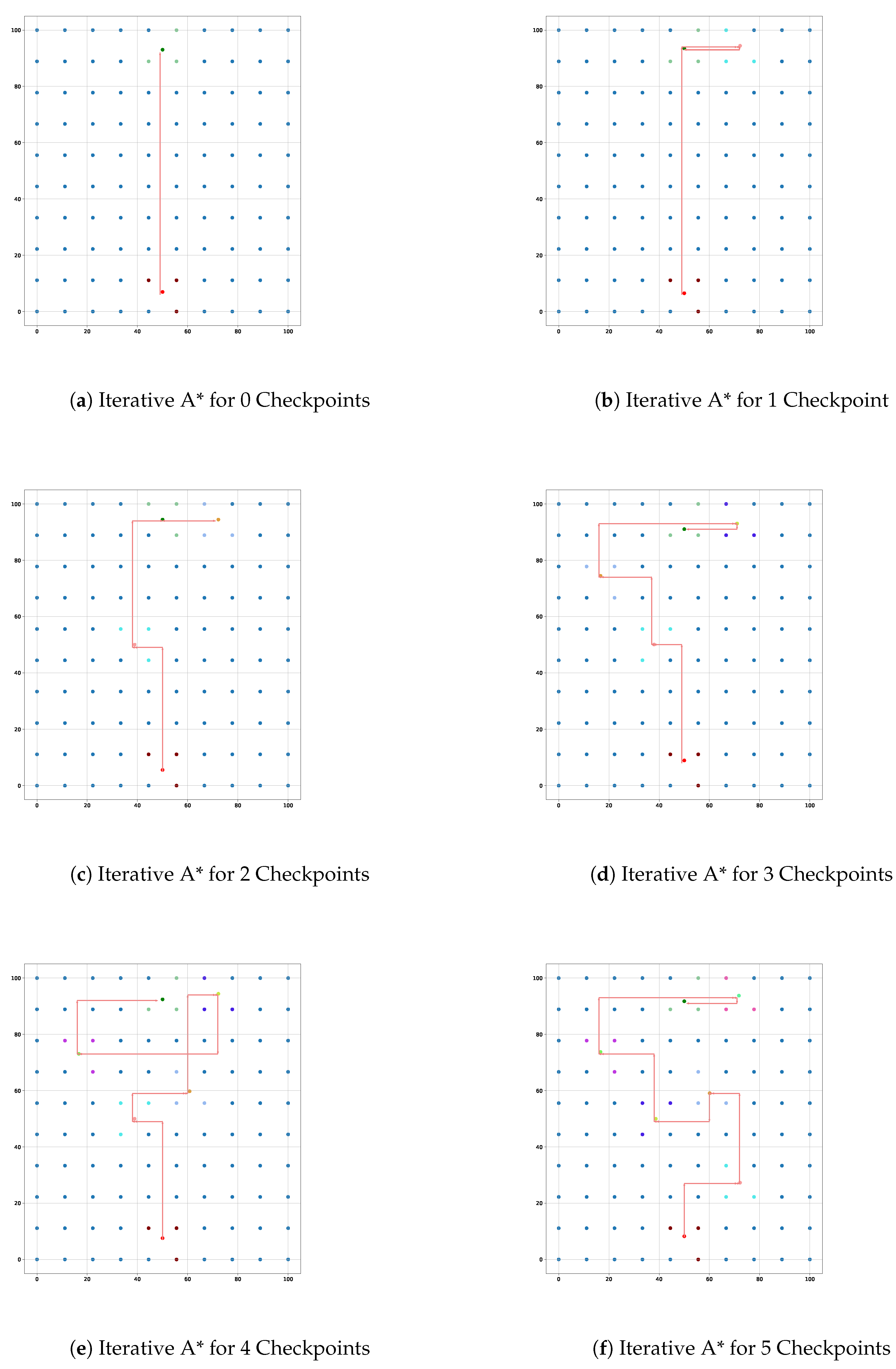
Figure 11.
Optimized paths derived by the Iterative A* algorithm for 0–5 checkpoints in Environment 2.
Figure 11.
Optimized paths derived by the Iterative A* algorithm for 0–5 checkpoints in Environment 2.
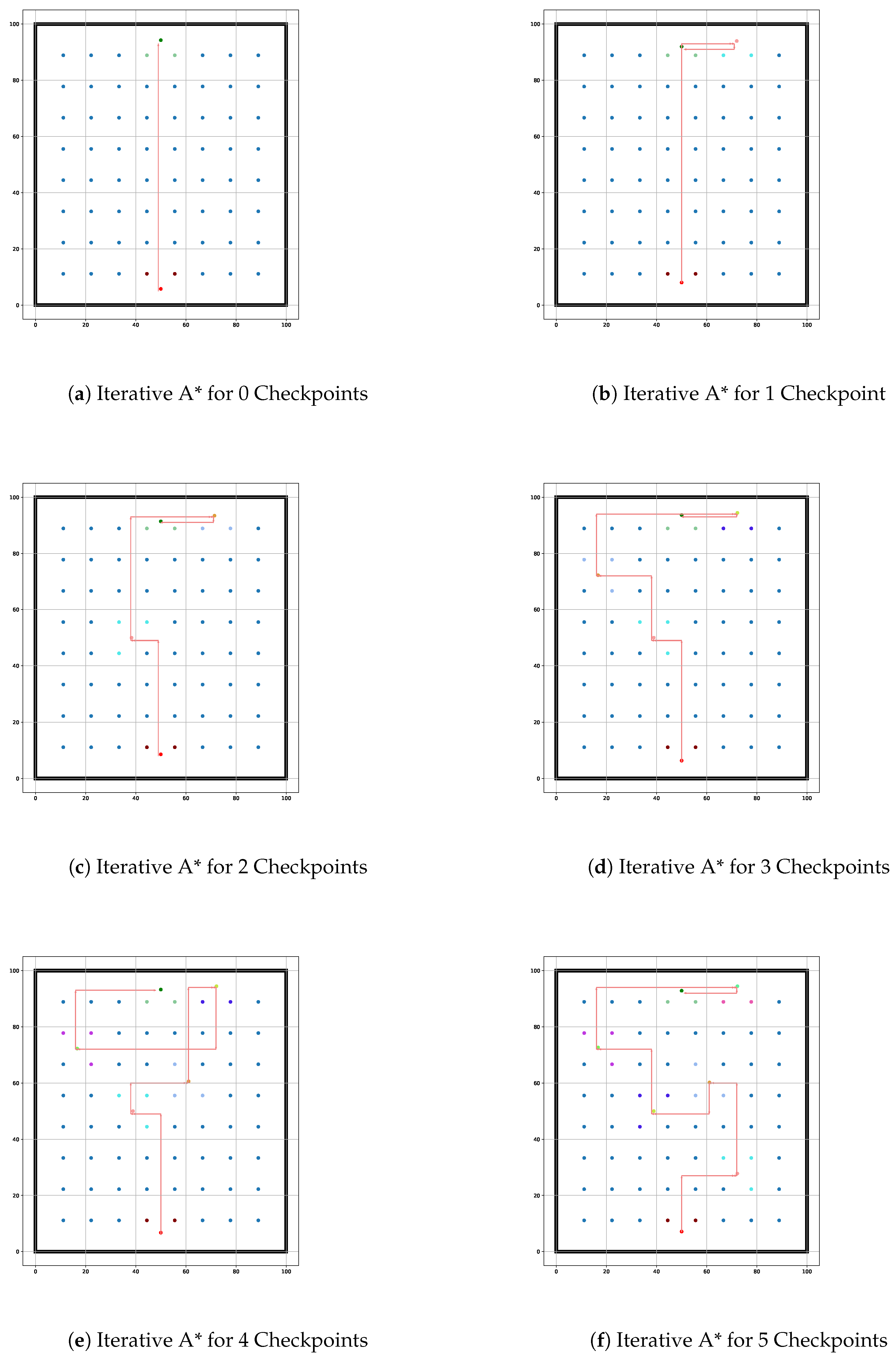
Figure 12.
Optimized paths derived by the Iterative A* algorithm for 0–5 checkpoints in Environment 3.
Figure 12.
Optimized paths derived by the Iterative A* algorithm for 0–5 checkpoints in Environment 3.
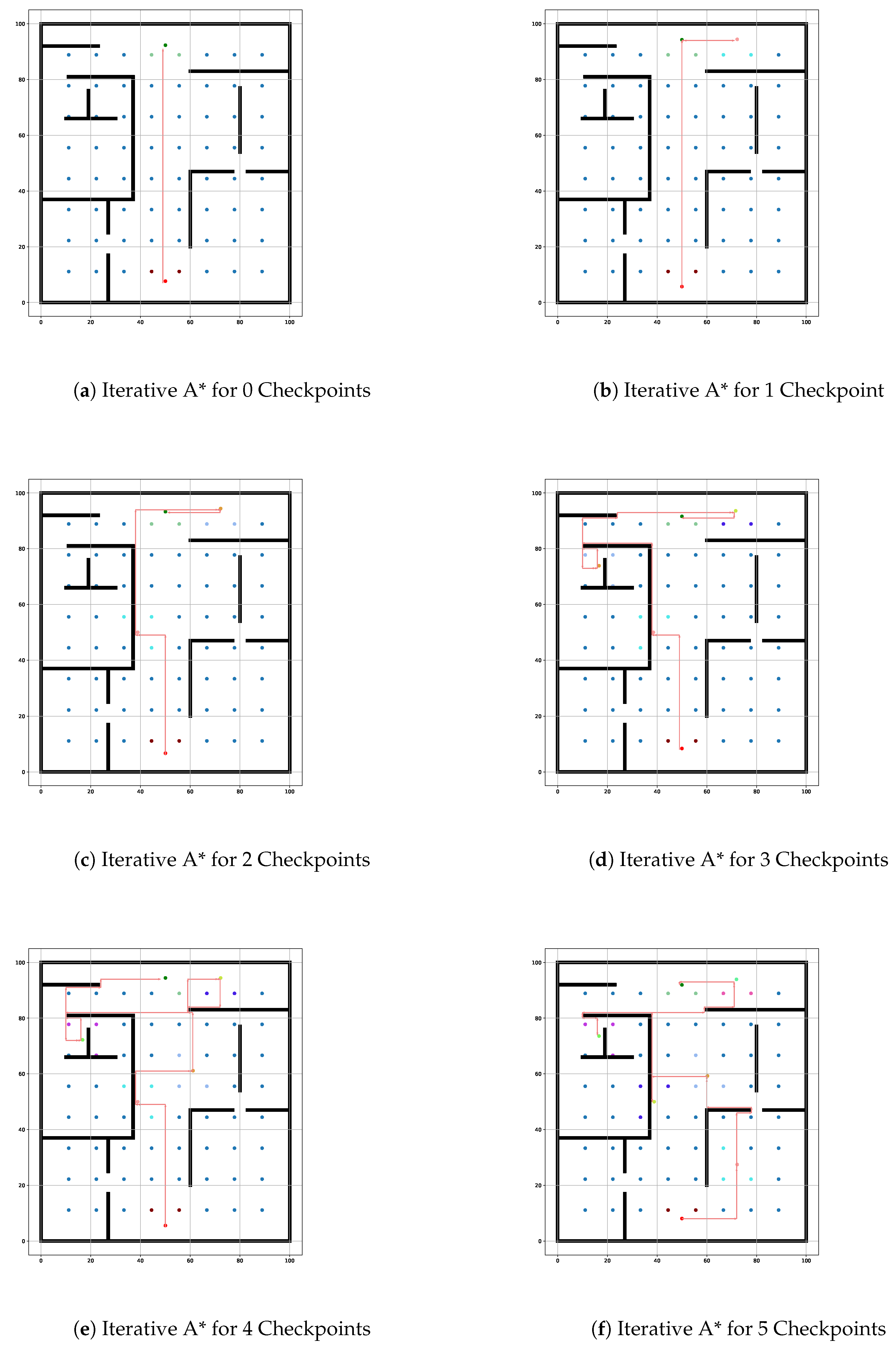
Table 3 presents the performance comparison between the Basic A* and Iterative A* algorithms in environment 1. The data reveals that the average algorithm execution time of the Iterative A* algorithm gets lowered compared to the Basic A* algorithm as the number of checkpoints increases and the Iterative A* algorithm also has lower memory consumption compared to the Basic A* which indicates that the proposed algorithm is optimized. The reduction in memory usage becomes significant when considering larger and more complex indoor environments where resources are limited and the Iterative A* algorithm can manage memory more efficiently while maintaining low execution time. The total path length used by both algorithms further demonstrates the superior performance of the Iterative A* algorithm. As the number of checkpoints increases, the ability of the proposed algorithm to reduce the path length also improves significantly. It is also able to reduce the number of turns and number of nodes required after redundant node removal. As there are no obstacles present in environment 1, the impact of the algorithm for reducing the number of turns and removing redundant nodes can be analyzed better in environment 3. Overall, the Iterative A* algorithm consistently demonstrates enhanced performance over the Basic A* algorithm, particularly as the number of checkpoints increases. The path lengths and the number of nodes evaluated also reveal a noticeable improvement in the Iterative A* algorithm, emphasizing its efficiency in navigating through multiple checkpoints.
In environment 2, the performance metrics are presented in Table 4. The results indicate that adding a border to the environment only impacts the memory usage and the average execution time of both algorithms while the rest of the performance metrics remain almost the same. There is a significant increase in average execution time and memory usage as the number of checkpoints grows in Environment 2 while the path length is almost the same as in Environment 1. However, the Iterative A* algorithm remains superior in terms of both memory and time efficiency compared to the Basic A* algorithm. The introduction of borders increases the complexity of pathfinding, but the Iterative A* still manages to maintain a lower node count and shorter paths.
Lastly, we evaluate the performance in Environment 3, as illustrated in Table 5. As obstacles have been introduced in Environment 3, there are blockades in the path that the path-planning algorithms must navigate around. The findings indicate that, while all the performance evaluation metrics increase with the number of checkpoints, the Iterative A* algorithm maintains its edge over the Basic A* algorithm. The table shows that the Iterative A* algorithm improves its optimization performance significantly in environments with obstacles when compared to the Basic A* algorithm. The data highlight that the Iterative A* algorithm not only handles the increased complexity more effectively but also delivers better performance in terms of path length and node reduction, illustrating its robustness in navigating challenging environments.
Overall, the simulation results across all conditions demonstrate a clear trend: the Iterative A* algorithm consistently outperforms the Basic A* algorithm, showcasing its effectiveness in a variety of pathfinding scenarios. The implications of these findings are significant, suggesting that the Iterative A* algorithm is better suited for applications requiring efficient navigation in complex environments.
5.2. Practical Evaluation
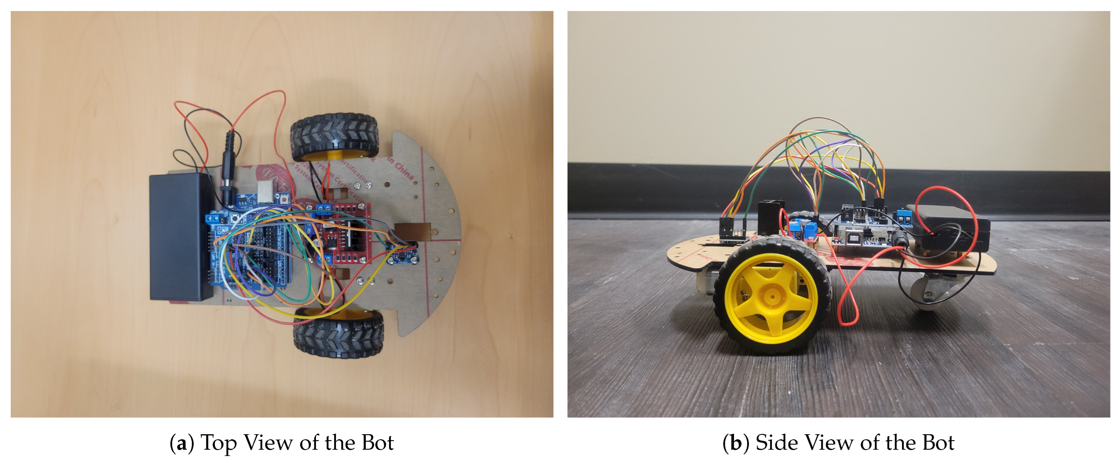
In order to validate the simulation results, a two-wheeled bot was run on the derived optimized path. The path data was transferred from the simulation environment to an Arduino microcontroller. Excluding the Arduino board, the bot only had an MPU-6050 sensor attached to it to ensure it made exactly 90-degree turns and followed the Manhattan path generated by the Iterative A* algorithm.
5.2.1. Practical Setup
Figure 13 shows the two-wheeled bot used for conducting the practical experiments. The microcontroller used the optimized path data to navigate through a scaled version of the simulated environment. Various runs of the bot demonstrated that it was able to navigate collision-free through the environment while moving through the desired checkpoints.
Figure 13.
Bot used for validating simulation results.(a) Top view of the bot.(b) Side view of the bot.
Figure 13.
Bot used for validating simulation results.(a) Top view of the bot.(b) Side view of the bot.
5.2.2. Practical Result
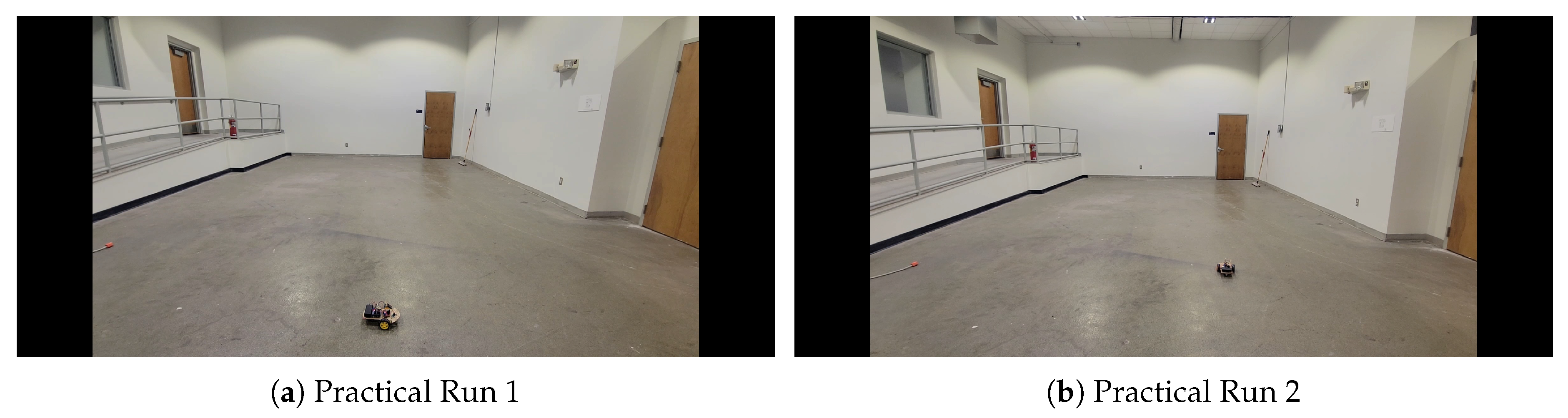
The practical evaluation of the Iterative A* algorithm was carried out using the two-wheeled bot described. The primary objective of the practical analysis was to assess the bot’s ability to navigate through a real environment by following the optimized path data derived from the simulation. Figure 14 shows an image of the bot navigating through the environment. The performance of the bot was compared against the simulation results to validate that the path provided by the Iterative A* algorithm ensures collision-free travel through the checkpoints with a minimal number of turns in the most optimized path. The overall evaluation confirmed that the optimized paths generated by the Iterative A* algorithm are practical and the bot can travel through the given path to reach the desired destination while moving through the checkpoints.
Figure 14.
Practical run images of the bot.(a) Practical Run 1. (b) Practical Run 2.
5.3. Quantitative Comparison
Table 6 shows the quantitative comparison between the Basic A* and the Iterative A* algorithm and highlights the improvements the proposed system makes compared to the basic algorithm in terms of key performance metrics—average execution time, memory usage, path length, the number of turns and the nodes remaining after node reduction—across the different environments. The formula used to calculate the improvement is shown in Equation 12. The proposed model was not compared with models present in other literature as the indoor environments differ from each other according to the arrangement of the indoor space, the grid size of the space being considered, the hardware used for simulating the environment, and the lack of evaluation of the models based on key performance metrics other than the path length. Adhering to so many external factors makes it extremely difficult to compare models from different literature with one another. For all the environments, it was observed that the number of turns and node reduction did not improve significantly unless obstacles were present in the environment.
Environments 1 and 2 have similar improvements for metrics such as path length, number of turns, and node reduction as both environments do not have any obstacles and the impact of having borders in the environment can be seen on the average execution time and the memory usage. Figure 15 shows the average execution times for the Basic A* and Iterative A* algorithms across three environments. It can be seen both from Figure 15 and Table 6 that for Environment 1, the Iterative A* algorithm can achieve a lower execution time of up to 35.14%, 31.52% for Environment 2, and 32.59% in Environment 3 compared to the Basic A*. This ensures the total algorithm run time is almost similar for both the algorithms even though the Iterative A* algorithm has a higher number of iterations. The Basic A* algorithm suffers from increasing execution times as it follows the sequence of checkpoints without dynamic optimization.
The proposed algorithm also optimizes the memory usage for all the environments and different numbers of checkpoints as shown in Table 6 and Figure 16. The proposed system can reduce memory usage up to 4.70% for Environment 1, 5.72% for Environment 2, and 5.73% for Environment 3. By efficiently reordering the checkpoint and minimizing unnecessary nodes, Iterative A* avoids unnecessary usage of memory that Basic A* incurs. The difference in memory usage becomes more apparent as the number of checkpoints increases and this reflects the Iterative A* algorithm’s ability to handle larger and more complex environments without consuming excessive resources.
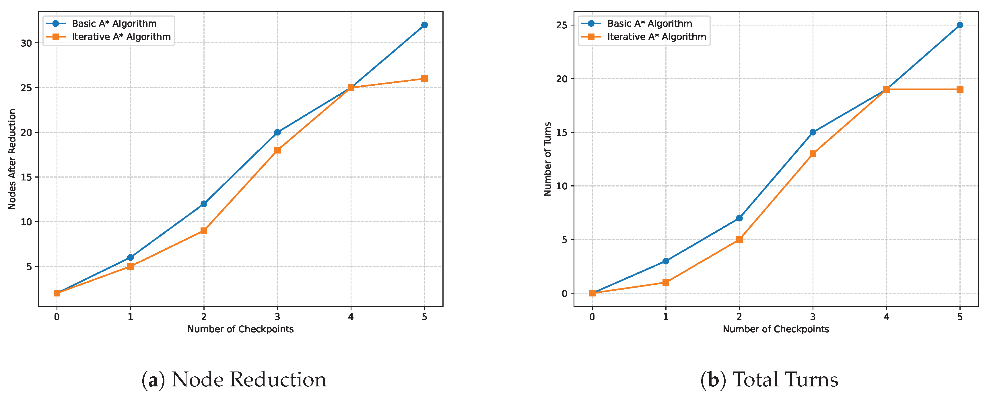
The comparison of path lengths shown in Figure 17, the number of turns and nodes after reduction is shown in Figure 18. The results from the Table 6 and the graphs show that the Iterative A* algorithm can achieve a higher path efficiency of up to 38.53% for both Environment 1 and Environment 2 while also achieving an improvement of 39.38% for Environment 3. In terms of reducing the number of turns, the proposed algorithm can achieve an improvement of up to 66.67% in Environment 3 but on average, the improvement is about 11.81% across all the Environments. In terms of obtaining the lowest number of nodes after node reduction, the Iterative A* algorithm also achieves optimization performance of up to 25% which is most significant in Environment 3 which has obstacles. The high path efficiency shows another critical advantage of the Iterative A* algorithm as it can minimize path length while significantly reducing the number of turns and the number of nodes explored.
Figure 15.
Average execution time comparison for (a) Environment 1. (b) Environment 2. (c) Environment 3.
Figure 15.
Average execution time comparison for (a) Environment 1. (b) Environment 2. (c) Environment 3.
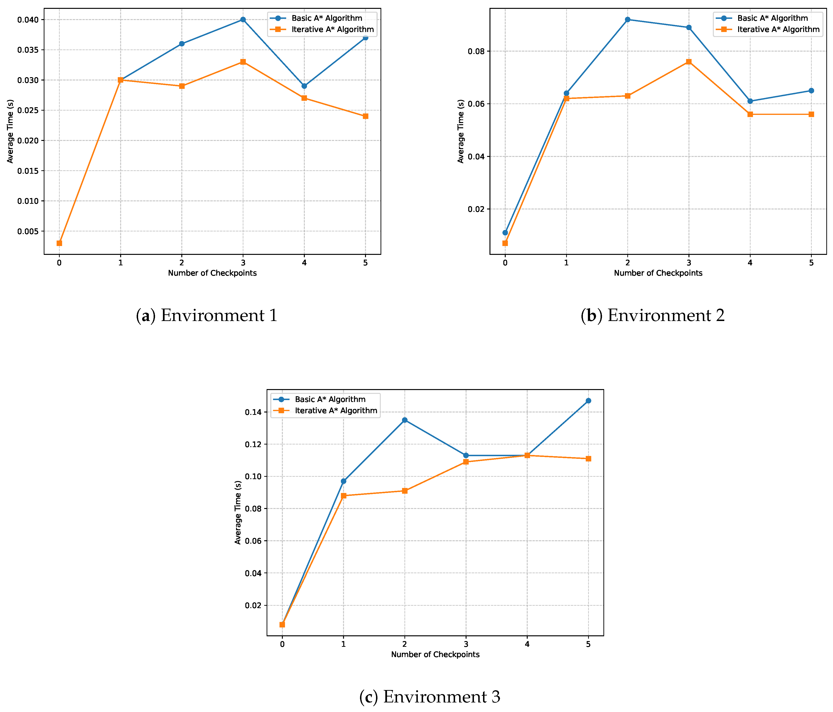
Figure 16.
Memory usage comparison for(a) Environment 1. (b) Environment 2. (c) Environment 3.
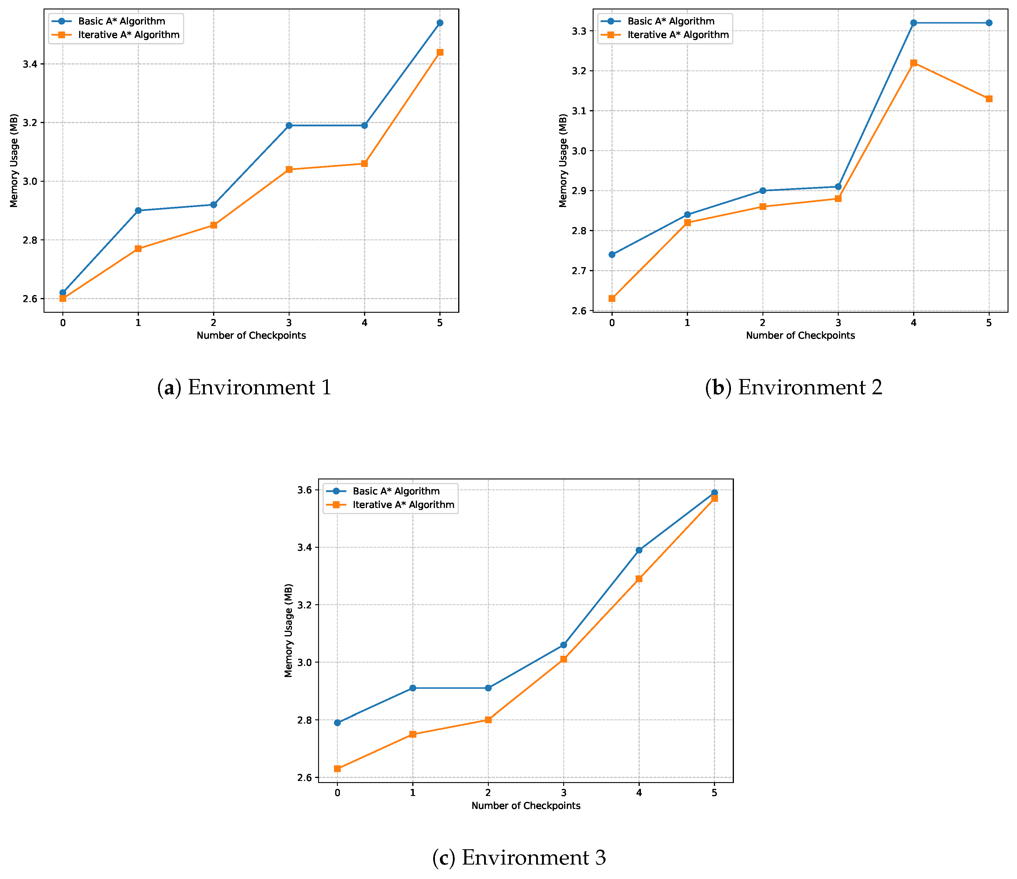
Figure 17.
Path length comparison for Environment 1, 2, and 3. (a) Environment 1. (b) Environment 2. (c) Environment 3.
Figure 17.
Path length comparison for Environment 1, 2, and 3. (a) Environment 1. (b) Environment 2. (c) Environment 3.
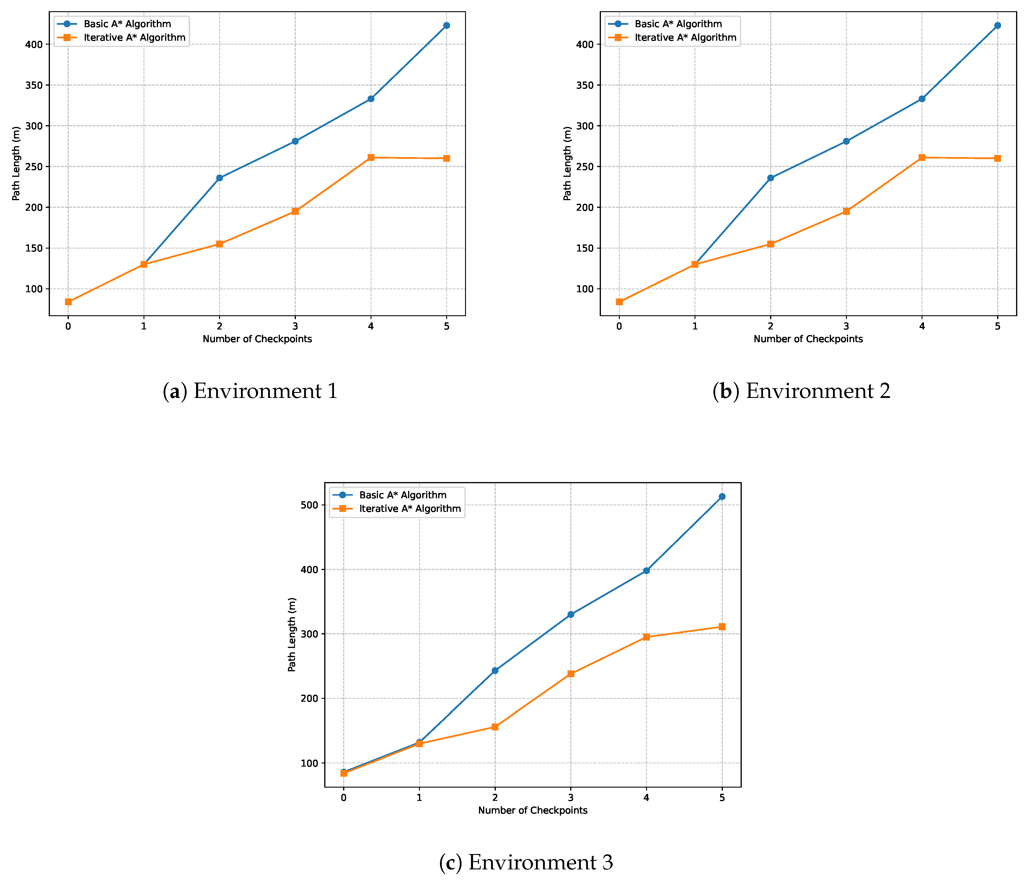
Figure 18.
Performace Metric Cpmparison for Environment 3. (a) Node Reduction. (b) Total Turns.
6. Discussion
In this section, we discuss the practical benefits and applications of the proposed algorithm, highlighting its organizational convenience, user-centric design, and resource efficiency.
6.1. Organizational Convenience
The proposed algorithm facilitates an organizational convenience by allowing organizations to utilize the simulated tool/code prior to implementing the actual algorithm. This initial phase focuses on mapping the physical indoor environment into a simulated grid layout. The grid is designed by uniformly distributing APs, enabling accurate indoor tracking via RSSI data.
To enhance user interaction, a GUI captures user inputs for barrier placement, dynamically reflecting any adjustments made. This approach ensures the placement of barriers does not exceed grid boundaries, facilitating the identification of the shortest path while avoiding obstacles. The dynamic GUI is illustrated in Figure 2, underscoring its role in fostering user engagement.
6.2. User Convenience
Enhancing user convenience is a central goal of the iterative A* algorithm and path optimization features. Following the determination of user and checkpoint coordinates, the iterative A* algorithm computes the most efficient route that navigates through all checkpoints to reach the final destination. The algorithm initiates with all nodes assigned an infinite cost and recalibrates based on user movement and proximity to checkpoints, as illustrated in equation (9). In the initial iteration, the algorithm identifies the nearest checkpoint based on the minimum steps required, effectively streamlining user navigation. The total iterations are defined by equation (10).
6.3. User Experience
To further enhance user experience, a node reduction algorithm is integrated to optimize the path determined by the iterative A* algorithm. This process reduces the number of nodes in the path, ensuring a smoother trajectory. The algorithm operates by evaluating straight-line paths and eliminating unnecessary nodes, as described in Algorithm 1.
The node reduction algorithm operates by assessing each node’s position relative to its neighbors, ensuring only relevant nodes remain. This careful consideration results in a path that maintains clarity while reducing computational overhead, ultimately benefiting the user’s navigation experience.
6.4. Cost Efficiency
The integration of RSSI-based trilateration and multiple checkpoints emphasizes cost efficiency, utilizing existing environmental elements without the need for additional infrastructure. The algorithm leverages RSSI data to estimate user positions and the locations of checkpoints. By identifying the three nearest APs based on the highest RSSI values, the algorithm calculates user and checkpoint coordinates using established trilateration equations.
This efficiency is further highlighted by the ability to manage multiple checkpoints, allowing users to traverse a dynamic path through the indoor environment while utilizing the same infrastructure. The algorithm recalibrates checkpoint distances based on user movement, ensuring that the path remains optimal.
6.5. Energy Efficiency
Energy efficiency is a critical feature of the proposed algorithm, setting it apart from traditional pathfinding methods. By focusing on minimizing computational overhead, the algorithm not only reduces execution time but also conserves the system’s energy resources, making it especially suitable for environments where battery-powered devices, such as robots or IoT systems, are in operation. This efficiency is achieved through the combination of iterative processing and node reduction techniques, both of which ensure that the algorithm calculates the shortest, most optimized paths with minimal resource consumption.
For instance, as seen in the simulation results presented in Table 3, Table 4, and Table 5, the Iterative A* consistently outperforms the Basic A* algorithm in terms of memory usage and path length. This optimization directly correlates with lower power consumption. A robot employing the Iterative A* algorithm, for example, would require fewer computational cycles to compute paths, resulting in reduced energy usage and extended operational time. The reduction in nodes, particularly after the node reduction phase, further amplifies this energy-saving characteristic, as fewer nodes translate to less processing and less strain on the hardware.
In addition, the algorithm’s efficiency in navigating complex environments, such as those with borders and static obstacles, showcases its ability to handle increased complexity without a proportional rise in energy consumption. By leveraging efficient pathfinding strategies, the algorithm avoids the pitfalls of traditional approaches that may unnecessarily expend energy recalculating redundant paths or processing excessive nodes. This distinction is vital in real-world applications, such as search-and-rescue operations or warehouse automation, where energy efficiency directly influences the system’s overall performance and sustainability.
6.6. Application
The proposed algorithm has a wide range of practical applications, particularly in environments where indoor navigation, positioning, and path optimization are critical. Its adaptability makes it highly suitable for industries and sectors that require efficient movement through complex indoor spaces while accounting for obstacles and varying layouts.
One key application is in automated warehouse management. In modern warehouses, robots and autonomous vehicles are increasingly used to streamline inventory management and product retrieval. By leveraging the proposed algorithm, these systems can dynamically navigate through warehouse aisles, avoiding barriers such as shelves or temporary obstructions. The use of RSSI-based trilateration ensures precise indoor positioning, enabling the algorithm to guide robots along the most efficient paths, even as the environment evolves due to rearranged inventory or new shelving configurations.
In healthcare facilities, such as hospitals or large medical centers, the algorithm can be used for guiding autonomous service robots or for providing real-time navigation assistance to both staff and visitors. These environments often feature complex layouts with multiple checkpoints—such as patient rooms, medical supply areas, or operating theaters—that must be reached efficiently. The proposed pathfinding and node reduction techniques ensure that essential services are delivered quickly, improving overall facility efficiency and enhancing patient care.
Another potential application lies in smart building management. Modern smart buildings rely on sophisticated systems to monitor and control various functions, from lighting and security to heating, ventilation, and air conditioning (HVAC). The proposed algorithm can be integrated into these systems to assist with tasks such as monitoring maintenance robots as they navigate through buildings to perform inspections or repairs. The ability to adapt to real-time changes in the environment ensures that these systems can operate continuously, even when unforeseen obstacles are introduced.
In the field of indoor rescue operations, particularly in situations where GPS signals are unavailable or unreliable, such as underground facilities or high-rise buildings, the algorithm can play a pivotal role. Rescue robots equipped with the algorithm can efficiently navigate disaster-stricken environments, locating survivors and delivering critical supplies. The combination of RSSI-based positioning and optimized pathfinding minimizes delays, which is essential when time-sensitive operations are involved.
Moreover, the algorithm finds practical use in indoor retail environments. Retailers are adopting technology-driven solutions to enhance customer experience, such as in-store navigation apps that guide customers to products in large, complex shopping centers or supermarkets. The proposed algorithm, when implemented in such systems, can offer precise directions while accounting for temporary store rearrangements or high-traffic areas, thus improving both customer satisfaction and operational efficiency.
Finally, in robotic swarm intelligence, the algorithm can serve as a key component in coordinating multiple robots working together in enclosed spaces. Swarm robots, used in tasks such as environmental monitoring, cleaning, or surveillance, need to efficiently cover an area without colliding with one another or missing any sections. The algorithm’s ability to handle multiple checkpoints and dynamically adjust paths based on real-time positioning allows for smooth and efficient coordination of these swarms, maximizing their coverage while minimizing operational costs.
6.7. Limitations and Future Considerations
While the proposed algorithm offers a robust solution for indoor positioning and navigation, several limitations must be acknowledged. First, the reliance on RSSI-based trilateration introduces inherent inaccuracies due to signal interference, multi-path effects, and fluctuations in signal strength within indoor environments. Such variations can reduce the precision of location estimates, particularly in dynamic environments with high-density barriers or reflective surfaces. To mitigate this, future research could explore the integration of alternative localization techniques, such as time-of-flight or angle-of-arrival measurements, which may provide more stable and accurate positioning in complex indoor environments.
Another limitation pertains to the scalability of the iterative A* algorithm when applied to large-scale environments. As the number of checkpoints increases, the computational cost and time required for path optimization grow exponentially. This limitation becomes especially apparent when dealing with highly cluttered environments where numerous obstacles must be accounted for. Future improvements could focus on optimizing the search space and incorporating hierarchical or multi-level pathfinding techniques, which would allow for faster computations without sacrificing accuracy. Additionally, leveraging parallel computing or cloud-based solutions could significantly reduce computation time, making the algorithm more suitable for real-time applications in larger, more complex environments.
The node reduction technique, while effective in simplifying paths, may occasionally eliminate nodes that contribute to smoother trajectories, particularly in environments where fine-tuned navigation is essential. Future research could explore adaptive node reduction strategies that preserve critical waypoints based on the specific characteristics of the environment, user preferences, or the robot’s physical constraints.
Moreover, the current algorithm does not account for dynamic changes in the environment, such as moving obstacles or alterations in the layout post-deployment. Addressing this limitation will require future work to integrate real-time environmental updates and re-calculations into the pathfinding process. This could involve combining machine learning techniques to predict obstacle movements or incorporating simultaneous localization and mapping (SLAM) to adaptively update the environment in real-time.
In terms of applicability, while the algorithm has been successfully implemented in a controlled simulation and later deployed on a microcontroller, its performance in real-world environments is still subject to constraints such as hardware limitations, sensor accuracy, and environmental unpredictability. Future work should explore more extensive real-world testing in various settings, including highly dynamic environments, to better assess the algorithm’s robustness and adaptability. Investigating the potential of integrating additional sensory inputs, such as lidar or computer vision, could further enhance the algorithm’s effectiveness in diverse real-world scenarios.
Finally, expanding the algorithm’s applicability to multi-agent systems is a promising direction. Coordinating multiple robots to navigate complex environments introduces additional challenges in path planning, collision avoidance, and resource optimization. Future research should focus on developing distributed algorithms that allow multiple agents to operate efficiently within the same environment, further extending the versatility of the proposed solution.
7. Conclusion
In this paper, we presented a comprehensive algorithm designed to optimize indoor positioning and navigation. By integrating multiple features such as RSSI-based trilateration, iterative A* pathfinding, and node reduction, the algorithm achieves both efficiency and accuracy in navigating dynamic environments. The user-friendly interface allows for seamless customization of barriers and checkpoints, ensuring the tool adapts to a wide range of indoor layouts. This adaptability, combined with the algorithm’s cost efficiency through the use of existing infrastructure, demonstrates its practical applicability.
Key performance metrics, including computational runtime, memory usage, and the number of steps required, highlight the algorithm’s balance between complexity and performance. Furthermore, the incorporation of a node reduction technique enhances the efficiency of pathfinding, reducing the computational burden without sacrificing precision. The algorithm’s deployment onto a microcontroller for real-world implementation bridges the gap between theoretical simulation and practical use.
In conclusion, this algorithm not only addresses the complexities of indoor navigation but also offers a scalable and adaptable solution that can be implemented across diverse environments. Its integration of user interaction, computational optimization, and real-world applicability positions it as a valuable contribution to the field of indoor positioning systems.
References
- Mendoza-Silva, G.M.; Torres-Sospedra, J.; Huerta, J. A meta-review of indoor positioning systems. Sensors 2019, 19, 4507.
- Research, G.V. Indoor Positioning And Navigation Market Size 2023.
- Ritchie, H.; Rodés-Guirao, L.; Mathieu, E.; Gerber, M.; Ortiz-Ospina, E.; Hasell, J.; Roser, M. Population Growth. Our World in Data 2023.
- Almadani, Y.; Plets, D.; Bastiaens, S.; Joseph, W.; Ijaz, M.; Ghassemlooy, Z.; Rajbhandari, S. Visible light communications for industrial applications-Challenges and potentials. Electronics 2020, 9, 2157.
- Pachni-Tsitiridou, O.; Fouskas, K. Location-Aware Technologies: How They Affect Customer Experience. Strategic Innovative Marketing and Tourism: 7th ICSIMAT, Athenian Riviera, Greece, 2018 2019, pp. 1199–1206.
- Storage, B. Warehouse Trends for 2022 and beyond 2022.
- Kolehmainen, V. Improve store efficiency with indoor positioning 2022.
- Elsanhoury, M.; Mäkelä, P.; Koljonen, J.; Välisuo, P.; Shamsuzzoha, A.; Mantere, T.; Elmusrati, M.; Kuusniemi, H. Precision positioning for smart logistics using ultra-wideband technology-based indoor navigation: A review. leee Access 2022, 10, 44413–44445.
- Laoudias, C.; Moreira, A.; Kim, S.; Lee, S.; Wirola, L.; Fischione, C. A survey of enabling technologies for network localization, tracking, and navigation. IEEE Communications Surveys & Tutorials 2018, 20, 3607–3644.
- Shukri, S.; Kamarudin, L.M. Device free localization technology for human detection and counting with RF sensor networks: A review. Journal of Network and Computer Applications 2017, 97, 157–174.
- Alamleh, H.; Alqahtani, A.A.S.; Gourd, J.; Mugasa, H. A weighting system for building RSS maps by crowdsourcing data from smartphones. In Proceedings of the 2020 International Conference on Computing, Networking and Communications (ICNC). IEEE, 2020, pp. 152–156.
- Papapostolou, A.; Chaouchi, H. RFID-assisted indoor localization and the impact of interference on its performance. Journal of Network and Computer Applications 2011, 34, 902–913.
- Wei, Z.; Chen, J.; Tang, H.; Zhang, H. RSSI-based location fingerprint method for RFID indoor positioning: a review. Nondestructive Testing and Evaluation 2024, 39, 3–31.
- Doğan, A.H.; Mumcu, T.V. Navigating in Complex Indoor Environments: A Comparative Study. Journal of Artificial Intelligence and Data Science 2023, 3, 124–137.
- Kulshrestha, T.; Saxena, D.; Niyogi, R.; Raychoudhury, V.; Misra, M. SmartITS: Smartphone-based identifica- tion and tracking using seamless indoor-outdoor localization. Journal of Network and Computer Applications 2017, 98, 97–113.
- Hernandez, S.M.; Bulut, E. Using perceived direction information for anchorless relative indoor localization. Journal of Network and Computer Applications 2020, 165, 102714.
- Shi, Y.; Shi, W.; Liu, X.; Xiao, X. An RSSI classification and tracing algorithm to improve trilateration-based positioning. Sensors 2020, 20, 4244.
- Liu, Z.; Liu, H.; Lu, Z.; Zeng, Q. A dynamic fusion pathfinding algorithm using delaunay triangulation and improved a-star for mobile robots. Ieee Access 2021, 9, 20602–20621.
- Zafari, F.; Gkelias, A.; Leung, K.K. A Survey of Indoor Localization Systems and Technologies. IEEE Communications Surveys & Tutorials 2019, 21, 2568–2599. [CrossRef]
- Alamleh, H.; AlQahtani, A.A.S. Architecture for continuous authentication in location-based services. In Proceedings of the 2020 International Conference on Innovation and Intelligence for Informatics, Computing and Technologies (3ICT). IEEE, 2020, pp. 1–4.
- Yaro, A.; Maly, E; Pražák, P. A Survey of the Performance-Limiting Factors of a 2-Dimensional RSS Fingerprinting-Based Indoor Wireless Localization System. Sensors 2023, 23, 2545. [CrossRef]
- 22 Rahman, A.B.M.M.; Li, T.; Wang, Y. Recent Advances in Indoor Localization via Visible Lights: A Survey. Sensors 2020, 20. [CrossRef]
- Dondo, J.; Villanueva, E; Garcia, D.; Vallejo, D.; Glez-Morcillo, C.; Lopez, J.C. Distributed fpga-based architecture to support indoor localisation and orientation services. Journal of network and computer applications 2014, 45, 181–190.
- Morar, A.; Moldoveanu, A.; Mocanu, L.; Moldoveanu, E; Radoi, LE; Asavei, V.; Gardener, A.; Butean, A. A Comprehensive Survey of Indoor Localization Methods Based on Computer Vision. Sensors 2020, 20. [CrossRef]
- Seco, F.; Prieto, J.C.; Ruiz, A.R.J.; Guevara, J. Compensation of Multiple Access Interference Effects in CDMA-Based Acoustic Positioning Systems. IEEE Transactions on Instrumentation and Measurement 2014, 63, 2368–2378. [CrossRef]
- Piontek, H.; Seyffer, M.; Kaiser, J. Improving the accuracy of ultrasound-based localisation systems. Personal Ubiquitous Comput. 2007, 11, 439–449. [CrossRef]
- Vera, R.; Ochoa, S.F.; Aldunate, R.G. EDIPS: an Easy to Deploy Indoor Positioning System to support loosely coupled mobile work. Personal and Ubiquitous Computing 2011, 15, 365–376.
- Obeidat, H.; Shuaieb, W.; Obeidat, O.; Abd-Alhameed, R. A review of indoor localization techniques and wireless technologies. Wireless Personal Communications 2021, 119, 289–327.
- Poulose, A.; Han, D.S. UWB indoor localization using deep leaming LSTM networks. Applied Sciences 2020, 10, 6290.
- Pahlavan, K.; Krishnamurthy, P. Evolution and impact of Wi-Fi technology and applications: A historical perspective. International Journal of Wireless Information Networks 2021, 28, 3–19.
- Retscher, G. Fundamental concepts and evolution of Wi-Fi user localization: An overview based on different case studies. Sensors 2020, 20, 5121.
- 32 Basri, C.; El Khadimi, A. Survey on indoor localization system and recent advances of WIFI fingerprinting technique. In Proceedings of the 2016 5th international conference on multimedia computing and systems (ICMCS). IEEE, 2016, pp. 253–259.
- Banin, L.; Schützberg, U.; Amizur, Y. Next generation indoor positioning system based on WiFi time of flight. In Proceedings of the Proceedings of the 26th International Technical Meeting of the Satellite Division of The Institute of Navigation (ION GNSS+ 2013), 2013, pp. 975–982.
- Abusubaih, M.; Rathke, B.; Wolisz, A. A dual distance measurement scheme for indoor IEEE 802.11 wireless local area networks. In Proceedings of the 2007 9th IFIP International Conference on Mobile Wireless Communications Networks, 2007, pp. 121–125. [CrossRef]
- Kumar, S.; Gil, S.; Katabi, D.; Rus, D. Accurate indoor localization with zero start-up cost. In Proceedings of the Proceedings of the 20th annual international conference on Mobile computing and networking, 2014, pp. 483–494.
- Kotaru, M.; Joshi, K.; Bharadia, D.; Katti, S. Spotfi: Decimeter level localization using wifi. In Proceedings of the Proceedings of the 2015 ACM conference on special interest group on data communication, 2015, pp. 269–282.
- Li, M.; Meng, Y.; Liu, J.; Zhu, H.; Liang, X.; Liu, Y.; Ruan, N. When CSI meets public WiFi Inferring your mobile phone password via WiFi signals. In Proceedings of the Proceedings of the 2016 ACM SIGSAC conference on computer and communications security, 2016, pp. 1068–1079.
- Nair, A.P.; Manoj, A.K.; V, A.; MP, N.; CA, A. Indoor Navigation System Using Wi-Fi RSSL. In Proceedings of the 2024 7th International Conference on Circuit Power and Computing Technologies (ICCPCT), 2024, Vol 1, pp. 954–959. [CrossRef]
- Zhuang, Y.; Syed, Z.; Georgy, J.; El-Sheimy, N. Autonomous smartphone-based WiFi positioning system by using access points localization and crowdsourcing. Pervasive and Mobile Computing 2015, 18, 118–136. [CrossRef]
- Yang, B.; Guo, L.; Guo, R.; Zhao, M.; Zhao, T. A novel trilateration algorithm for RSSI-based indoor localization. IEEE Sensors Journal 2020, 20, 8164–8172.
- Karur, K.; Sharma, N.; Dharmatti, C.; Siegel, J.E. A survey of path planning algorithms for mobile robots. Vehicles 2021, 3, 448–468.
- 42 Ismail, A.; Sheta, A.; AL-Weshah, M. A mobile robot path planning using genetic algorithm in static environment. Journal of Computer Science 2008, 4, 341–344.
- Debnath, D.; Vanegas, F.; Sandino, J.; Hawary, A.F.; Gonzalez, E. A Review of UAV Path-Planning Algorithms and Obstacle Avoidance Methods for Remote Sensing Applications. Remote Sensing 2024, 16, 4019.
- Liu, L.; Wang, X.; Yang, X.; Liu, H.; Li, J.; Wang, P. Path planning techniques for mobile robots: Review and prospect. Expert Systems with Applications 2023, 227, 120254. https//doi.org/https://doi.org/10.1016/j. eswa.2023.120254.
- Wang, R.; Lu, Z.; Jin, Y.; Liang, C. Application of A* algorithm in intelligent vehicle path planning. Mathematical Models in Engineering 2022, 8, 82–90.
- Yu, X.; Chen, W.N.; Gu, T.; Yuan, H.; Zhang, H.; Zhang, J. ACO-A*: Ant Colony Optimization Plus A* for 3-D Traveling in Environments With Dense Obstacles. IEEE Transactions on Evolutionary Computation 2019, 23, 617–631. [CrossRef]
- Huang, C.; Zhao, Y.; Zhang, M.; Yang, H. APSO: An A*-PSO Hybrid Algorithm for Mobile Robot Path Planning. IEEE Access 2023, 11, 43238–43256. [CrossRef]
- 48 Fan, T.; Wang, D.; Liu, W.; Pan, J. Crowd-driven mapping, localization and planning. In Proceedings of the Experimental Robotics: The 17th International Symposium. Springer, 2021, pp. 354–368.
- Liu, T.; Li, H.; Lu, H.; Cheema, M.A.; Shou, L. Towards crowd-aware indoor path planning (extended version). arXiv preprint arXiv:2104.05480 2021.
- Hewawasam, H.; Ibrahim, M.Y.; Appuhamillage, G.K. Past, present and future of path-planning algorithms for mobile robot navigation in dynamic environments. IEEE Open Journal of the Industrial Electronics Society 2022, 3, 353–365.
- Yuan, C.; Zhang, W.; Liu, G.; Pan, X.; Liu, X. A heuristic rapidly-exploring random trees method for manipulator motion planning. IEEE access 2019, 8, 900–910.
- 52 Bruce, J.; Veloso, M. Real-time randomized path planning for robot navigation. In Proceedings of the IEEE/RSJ international conference on intelligent robots and systems. IEEE, 2002, Vol. 3, pp. 2383–2388.
- Suryaprakash, S.; Thirumoorthi, P.; Viswanathan, T. Development of an Indoor Navigation System for Mobile Robots Using Sensor Fusion and Path Planning Algorithms. In Proceedings of the 2023 2nd International Conference on Advancements in Electrical, Electronics, Communication, Computing and Automation (ICAECA), 2023, pp. 1–6. [CrossRef]
- Kantawong, S. Indoor Fire Evacuation Guidance Using QR Code Vision-based combine with an Adaptive Routing Localization. In Proceedings of the 2022 International Electrical Engineering Congress (iEECON), 2022, pp. 1–4.
- Liu, M.; Zou, S.; Fu, X.; Xie, C. Research on Fusion Path Planning Method Based on UWB Positioning. In Proceedings of the 2023 IEEE International Conference on Mechatronics and Automation (ICMA), 2023, pp. 929–934. [CrossRef]
- Wang, X.; Ma, X., Zhu, S.; Zhang, K.; Sun, Y. Research on Localization and Path Planning of Indoor Robot Based on ROS. In Proceedings of the 2021 International Conference on Computer Information Science and Artificial Intelligence (CISAI), 2021, pp. 793–796.
- Dong, J.; Wang, H.; Pan, Q.K. An Improved Multi-objective Evolutionary Algorithm for A Robot Detect Path Planning Problem. In Proceedings of the 2022 41st Chinese Control Conference (CCC), 2022, pp. 2071–2076. [CrossRef]
- Lee, J.; Park, H.; Kim, Y.; Park, C.G.; Lee, J.H. Multi-Level Indoor Path Planning and Clearance-Based Path Optimization for Search and Rescue Operations. IEEE Access 2023, 11, 40930–40943. [CrossRef]
- Chitsobhuk, O.; Warunsin, K.; Udomthanapong, S. Multidestination Indoor Navigation Using Path Planning and WiFi Fingerprint Localization. In Proceedings of the 2018 3rd International Conference on Computer and Communication Systems (ICCCS), 2018, pp. 406–410. [CrossRef]
- AlQahtani, A.A.S; Alamleh, H.; Gourd, J. OEISUA: Zero Effort Indoor Secure User Authentication. IEEE Access 2020, 8,79069-79078. [CrossRef]
Figure 1.
Flowchart of the Proposed Path Planning Algorithm
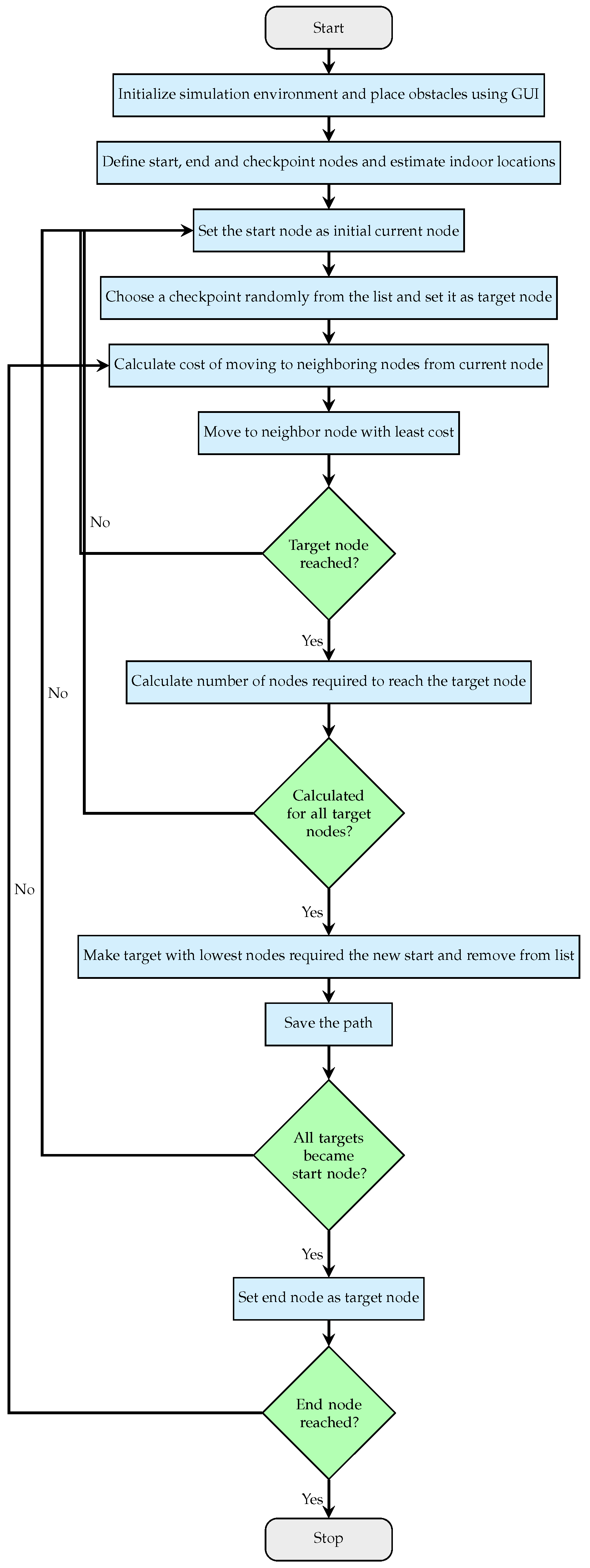
Figure 2.
The different simulation environments generated using the GUI.
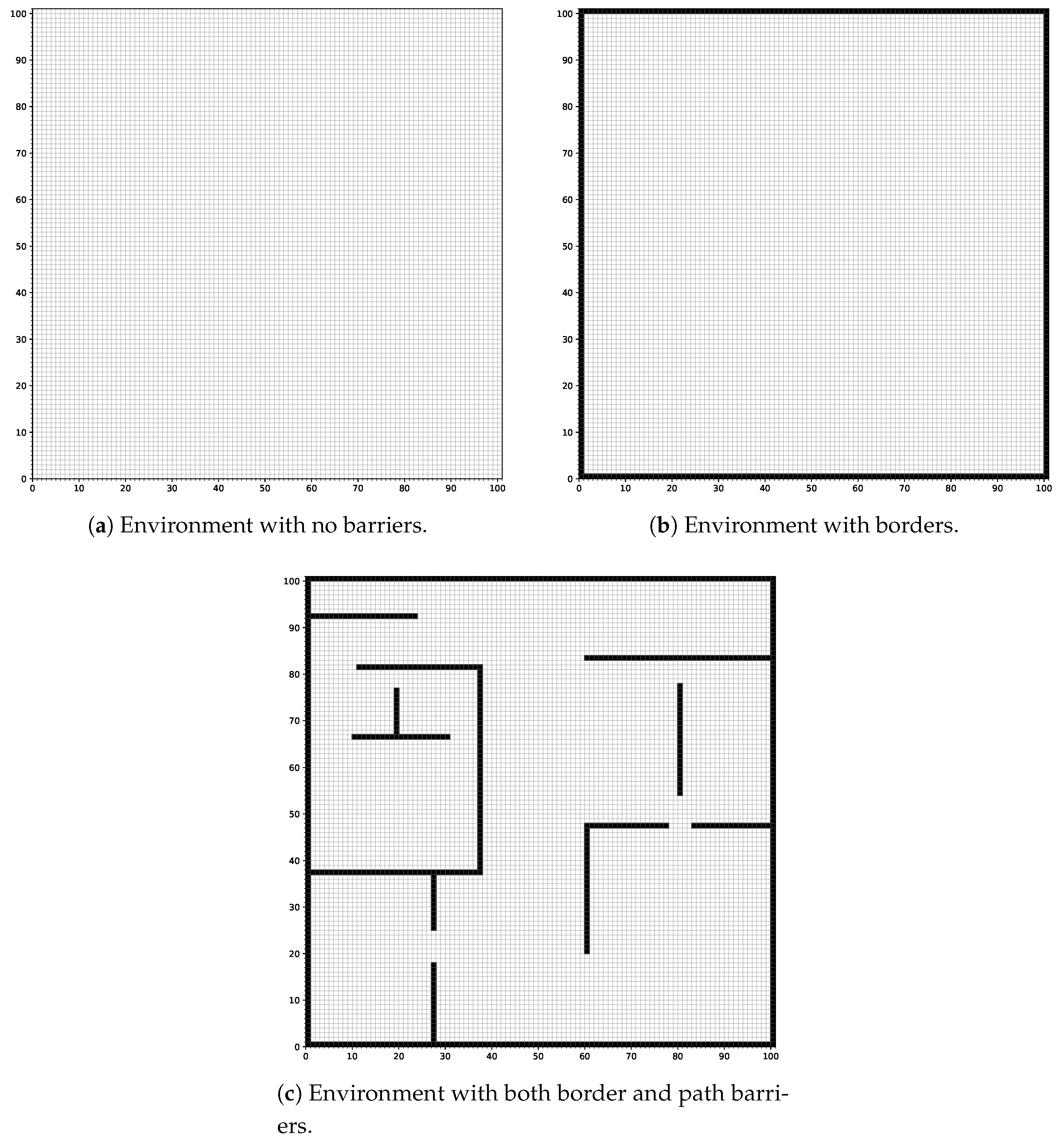
Figure 3.
Simulation environment legends.

Figure 4.
The different simulation environments generated using the GUI.
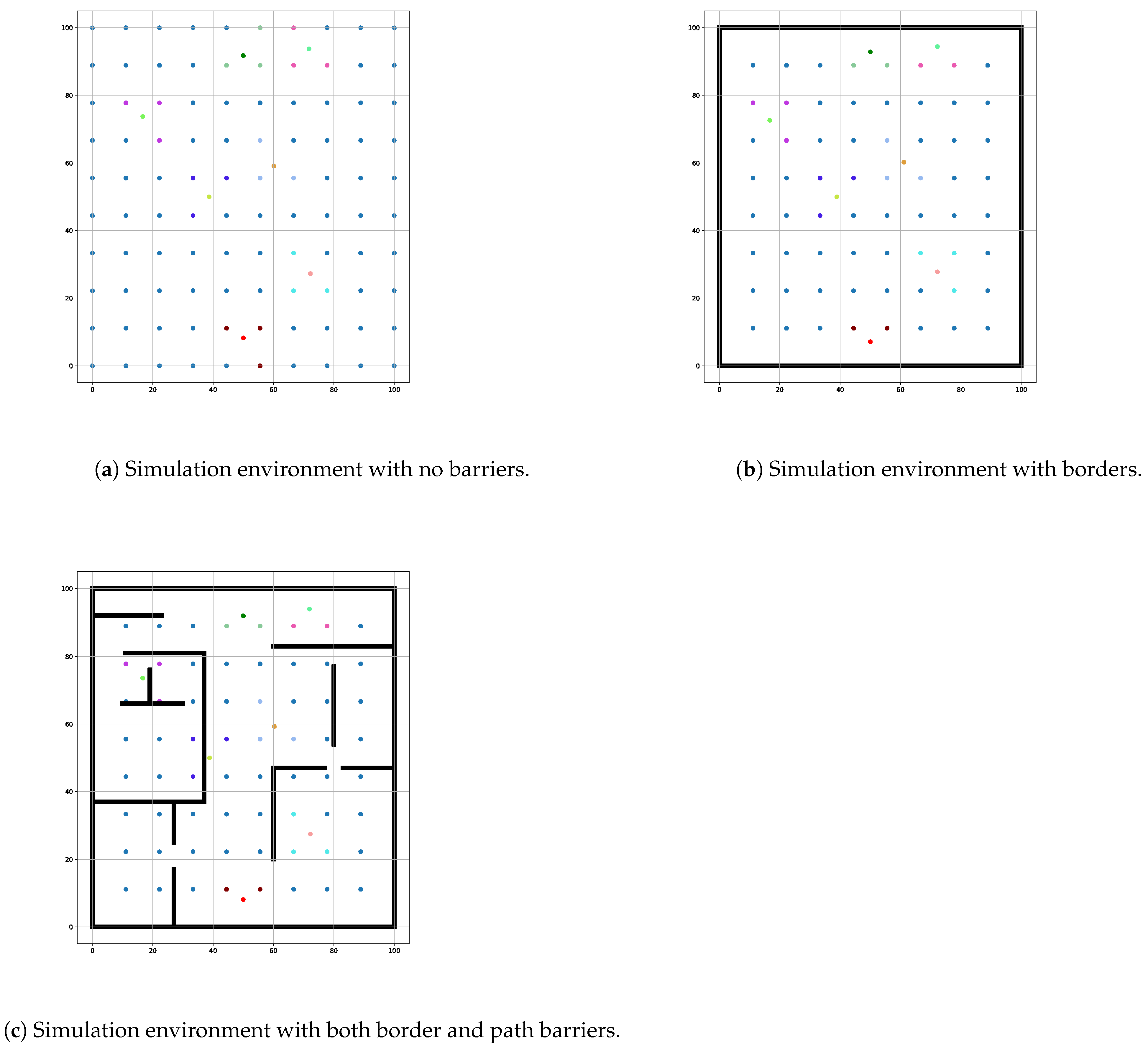
Figure 5.
The initial path given by the iterative A* algorithm in the different simulation environments. (a) Path found in an environment with no barriers. (b) Path found in an environment with borders. (c) Path found in an environment with both border and path barriers.
Figure 5.
The initial path given by the iterative A* algorithm in the different simulation environments. (a) Path found in an environment with no barriers. (b) Path found in an environment with borders. (c) Path found in an environment with both border and path barriers.


Table 1.
Comparison with The Discussed Works, Where ✓: Feature Supported, and ✗: Not Supported
| Study | Adjustable | Traceability | Waypointing | Navigational | Optimization |
|---|---|---|---|---|---|
| [25,26,27,33,34,35,36,37,38,39,40] | ✗ | ✓ | ✗ | ✗ | ✗ |
| [42] | ✗ | ✗ | ✗ | ✓ | ✗ |
| [45,47,51,52] | ✗ | ✗ | ✗ | ✓ | ✓ |
| [46,57,58] | ✗ | ✗ | ✓ | ✓ | ✓ |
| [48,49,53,54,55] | ✗ | ✓ | ✗ | ✓ | ✓ |
| [56] | ✓ | ✓ | ✗ | ✓ | ✓ |
| [59] | ✗ | ✓ | ✓ | ✓ | ✓ |
| Ours | ✓ | ✓ | ✓ | ✓ | ✓ |
Table 2.
Indoor Localization Results
| Indoor Map | Estimated Coordinates () | Actual Coordinates() | Error (%) |
|---|---|---|---|
| (50, 8) | (50, 10) | 3.33 | |
| (71, 93) | (69, 91) | 2.5 | |
| (38, 49) | (37, 51) | 3.41 | |
| Environment 1 | (16, 73) | (18, 76) | 5.32 |
| (60, 59) | (57, 56) | 5.31 | |
| (72, 27) | (72, 26) | 1.02 | |
| (50, 91) | (50, 90) | 0.71 | |
| (50, 7) | (50, 10) | 5.0 | |
| (72, 94) | (69, 91) | 3.75 | |
| (38, 49) | (37, 51) | 3.41 | |
| Environment 2 | (16, 72) | (18, 76) | 6.38 |
| (61, 60) | (57, 56) | 7.08 | |
| (72, 27) | (72, 26) | 1.02 | |
| (50, 92) | (50, 90) | 1.43 | |
| (50, 8) | (50, 10) | 3.33 | |
| (71, 93) | (69, 91) | 2.5 | |
| (38, 49) | (37, 51) | 3.41 | |
| Environment 3 | (16, 73) | (18, 76) | 5.32 |
| (60, 59) | (57, 56) | 5.31 | |
| (72, 27) | (72, 26) | 1.02 | |
| (49, 91) | (50, 90) | 1.43 |
Table 3.
Performance Comparison of Basic A* and Iterative A* Algorithms In Environment 1
| Performance Type | Basic A* Algorithm | Iterative A* Algorithm | ||||||||||
|---|---|---|---|---|---|---|---|---|---|---|---|---|
| Checkpoints | 0 | 1 | 2 | 3 | 4 | 5 | 0 | 1 | 2 | 3 | 4 | 5 |
| Average Time (s) | 0.003 | 0.030 | 0.036 | 0.040 | 0.029 | 0.037 | 0.003 | 0.030 | 0.029 | 0.033 | 0.027 | 0.024 |
| Algorithm Iterations | 1 | 2 | 3 | 4 | 5 | 6 | 1 | 2 | 4 | 7 | 11 | 16 |
| Memory usage (MB) | 2.62 | 2.90 | 2.92 | 3.19 | 3.19 | 3.54 | 2.60 | 2.77 | 2.85 | 3.04 | 3.06 | 3.44 |
| Path Length (m) | 84 | 130 | 236 | 281 | 333 | 423 | 84 | 130 | 155 | 195 | 261 | 260 |
| Turns | 0 | 3 | 5 | 7 | 9 | 11 | 0 | 3 | 3 | 7 | 9 | 11 |
| Nodes | 85 | 131 | 237 | 282 | 334 | 424 | 85 | 131 | 156 | 196 | 262 | 261 |
| Nodes After Reduction | 2 | 6 | 9 | 12 | 15 | 18 | 2 | 6 | 8 | 12 | 15 | 18 |
Table 4.
Performance Comparison of Basic A* and Iterative A* Algorithms In Environment 2
| Performance Type | Basic A* Algorithm | Iterative A* Algorithm | ||||||||||
|---|---|---|---|---|---|---|---|---|---|---|---|---|
| Checkpoints | 0 | 1 | 2 | 3 | 4 | 5 | 0 | 1 | 2 | 3 | 4 | 5 |
| Average Time (s) | 0.011 | 0.064 | 0.092 | 0.089 | 0.061 | 0.065 | 0.007 | 0.062 | 0.063 | 0.076 | 0.056 | 0.056 |
| Algorithm Iterations | 1 | 2 | 3 | 4 | 5 | 6 | 1 | 2 | 4 | 7 | 11 | 16 |
| Memory usage (MB) | 2.74 | 2.84 | 2.90 | 2.91 | 3.32 | 3.32 | 2.63 | 2.82 | 2.86 | 2.88 | 3.22 | 3.13 |
| Path Length (m) | 84 | 130 | 236 | 281 | 333 | 423 | 84 | 130 | 155 | 195 | 261 | 260 |
| Turns | 0 | 3 | 5 | 7 | 9 | 11 | 0 | 3 | 3 | 7 | 9 | 11 |
| Nodes | 85 | 131 | 237 | 282 | 334 | 424 | 85 | 131 | 156 | 196 | 262 | 261 |
| Nodes After Reduction | 2 | 6 | 9 | 12 | 15 | 18 | 2 | 6 | 8 | 12 | 15 | 18 |
Table 5.
Performance Comparison of Basic A* and Iterative A* Algorithms In Environment 3
| Performance Type | Basic A* Algorithm | Iterative A* Algorithm | ||||||||||
|---|---|---|---|---|---|---|---|---|---|---|---|---|
| Checkpoints | 0 | 1 | 2 | 3 | 4 | 5 | 0 | 1 | 2 | 3 | 4 | 5 |
| Average Time (s) | 0.008 | 0.097 | 0.135 | 0.113 | 0.113 | 0.147 | 0.008 | 0.088 | 0.091 | 0.109 | 0.113 | 0.111 |
| Algorithm Iterations | 1 | 2 | 3 | 4 | 5 | 6 | 1 | 2 | 4 | 7 | 11 | 16 |
| Memory usage (MB) | 2.79 | 2.91 | 2.91 | 3.06 | 3.39 | 3.59 | 2.63 | 2.75 | 2.80 | 3.01 | 3.29 | 3.57 |
| Path Length (m) | 86 | 132 | 243 | 330 | 398 | 513 | 84 | 130 | 156 | 238 | 295 | 311 |
| Turns | 0 | 3 | 7 | 15 | 19 | 25 | 0 | 1 | 5 | 13 | 19 | 19 |
| Nodes | 87 | 133 | 244 | 331 | 399 | 514 | 85 | 131 | 157 | 239 | 296 | 312 |
| Nodes After Reduction | 2 | 6 | 12 | 20 | 25 | 32 | 2 | 5 | 9 | 18 | 25 | 26 |
Table 6.
Quantitative Improvement Comparison of Iterative A* Over Basic A* Algorithm
| Environment | Checkpoints | Average Time (%) | Memory Usage (%) | Path Length (%) | Turns (%) | Nodes Reduction (%) |
|---|---|---|---|---|---|---|
| Environment 1 | 0 | 0.00 | 0.76 | 0.00 | 0.00 | 0.00 |
| 1 | 0.00 | 4.48 | 0.00 | 0.00 | 0.00 | |
| 2 | 19.44 | 2.40 | 34.32 | 40.00 | 11.11 | |
| 3 | 17.50 | 4.70 | 30.60 | 0.00 | 0.00 | |
| 4 | 6.90 | 4.08 | 21.62 | 0.00 | 0.00 | |
| 5 | 35.14 | 2.82 | 38.53 | 0.00 | 0.00 | |
| Environment 2 | 0 | 36.36 | 4.01 | 0.00 | 0.00 | 0.00 |
| 1 | 3.13 | 0.70 | 0.00 | 0.00 | 0.00 | |
| 2 | 31.52 | 1.38 | 34.32 | 40.00 | 11.11 | |
| 3 | 14.61 | 1.03 | 30.60 | 0.00 | 0.00 | |
| 4 | 8.20 | 3.01 | 21.62 | 0.00 | 0.00 | |
| 5 | 13.85 | 5.72 | 38.53 | 0.00 | 0.00 | |
| Environment 3 | 0 | 0 | 5.73 | 2.33 | 0.00 | 0.00 |
| 1 | 9.28 | 5.50 | 1.52 | 66.67 | 16.67 | |
| 2 | 32.59 | 3.78 | 35.80 | 28.57 | 25.00 | |
| 3 | 3.54 | 1.63 | 27.88 | 13.33 | 10.00 | |
| 4 | 0.00 | 2.95 | 25.88 | 0.00 | 0.00 | |
| 5 | 24.49 | 0.56 | 39.38 | 24.00 | 18.75 |
Disclaimer/Publisher’s Note: The statements, opinions and data contained in all publications are solely those of the individual author(s) and contributor(s) and not of MDPI and/or the editor(s). MDPI and/or the editor(s) disclaim responsibility for any injury to people or property resulting from any ideas, methods, instructions or products referred to in the content. |
© 2025 by the authors. Licensee MDPI, Basel, Switzerland. This article is an open access article distributed under the terms and conditions of the Creative Commons Attribution (CC BY) license (http://creativecommons.org/licenses/by/4.0/).
Copyright: This open access article is published under a Creative Commons CC BY 4.0 license, which permit the free download, distribution, and reuse, provided that the author and preprint are cited in any reuse.


