
Submitted:
13 January 2025
Posted:
14 January 2025
You are already at the latest version
Abstract
In this paper we formulate a Classical layer resolving finite difference scheme to solve a
system of two singularly perturbed time-dependent problems with discontinuity occurs at
(y; t) in the source terms and Robin initial conditions. The delay term occurs in the spatial
variable and leading term of spatial derivative of each equation is multiplied by a distinct
small positive perturbation parameter, inducing layer behaviors in the solution domain. The
formulation of finite difference scheme involves discretization of temporal and spatial axis
by uniform and piecewise uniform meshes respectively. Due to presence of perturbation
parameters, discontinuous source terms and delay terms, initial and interior layers occur in
the solution domain. In order to capture the abrupt change occurs due to the behavior of
these layers, the solution is further decomposed into two components. Layer functions are
also formulated in accordance with layer behavior. At last, to bolster the numerical scheme,
an example problem is computed to prove efficacy of our scheme.
Keywords:
finite difference scheme
; singularly perturbed problems
; discontinuous source terms
; spatial delay
; Robin initial conditions
; interior layers
MSC: 35L03; 65M06; 65M12; 65M15; 65M22; 65M50
1. Introduction
Solving Singular perturbation problems (SPPs) is very tedious due to presence of layer phenomena in the solution domain and presence of discontinuity in the source term makes it further more difficult since the solution behaves uneven or non–smooth at the discontinuity point. This leads to formation of interior layer at the region in the domain where the discontinuity occurs. To tackle such difficulties in estimating the solution of SPPs, classical numerical schemes are modified in such a way it uses highly refined meshes (i.e., Shishkin mesh, Bakhvalov mesh) to give numerical approximation by preserving the monotonicity of the original problem. Many specialized techniques are introduced by researches across the globe in order to overcome difficulties arising in solving SPPs.
Abagero et al. [1] employed a fitted nonstandard numerical method to solve SPPs with Robin type boundary conditions and discontinuous source terms. Sahoo & Gupta [8] employed a first–order upwind scheme on a Shishkin Mesh to sol-ve convection–diffusion SPPs with discontinuous convective and source terms. They further employed Richardson extrapolation Scheme to enhance order of convergence. Singh et al. [10] have devised a Spline-based numerical technique such Crank–Nicolson scheme and trigonometric B–spline basis function to solve two–parameter SPPs with discontinuity in convection coefficient and source term. Richardson extrapolation scheme is used by the authors to enhance accuracy in spatial direction. Chawla et al. [5] employed a backward difference scheme on Shishkin and Bakhvalov meshes to solve first order Singularly perturbed differential equations (SPDEs) with discontinuous source term. Cen et al. [4] developed a quadratic B–spline collocation method on Shishkin–type mesh to solve semilinear reaction–diffusion SPP with discontinuous source term. Soundararajan et al. [11] employed backward Euler Method for time discretization and streamline–diffusion Finite Element Method (FEM) on Shishkin mesh to solve 1D parabolic SPPs with discontinuous source term. Ajay Singh Rathore & Vembu Shanthi [2] proposes an exponentially fitted mesh method to solve the singularly perturbed Fredholm Integro–differential equation with discontinuous source term. Paramasivam et al. [7] formulated a classical numerical scheme employing finite difference Method on Shishkin mesh to solve second–order reaction-diffusion SPPs with discontinuous source terms.
Inspired from pioneer research outlined in the above literature review and method formulated in [9], we have crafted a classical layer resolving finite difference scheme (FDS) to solve a system of two time-dependent delay SPPs with a discontinuity occurring at in the source terms and Robin initial conditions. The subsequent section outlines organizing framework of the paper. Section 2 outlines the problem statement. Solution components and layer functions are discussed in Section 3. In Section 4, bounds on solutions and its components are derived. Discrete solution components and error estimates are discussed in Section 5. Numerical scheme is constructed for an example problem in Section 6.
2. The Problem Statement
In this article, we consider the following problem with discontinuous source term in the domain
with
The following symbols represent the key notation utilized throughout the text.
. , and . For all ,,,with, and The jump at is denoted by a function where . The functions are assumed to be in and can operate on functions in the domain . Furthermore, for all , the components of and respectively satisfy the following conditions
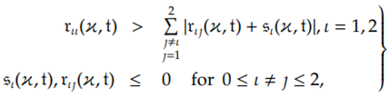 and for any positive number ,
The function is discontinuous at due to a finite jump. So the solution does not possess a continuous first order derivative at . We have to deal with two different cases due to the presence of in the domain.
Case 1:
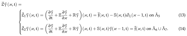
The problem (1) can be reformulated as
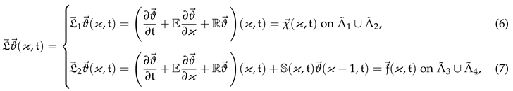 where .
For the problem (6) and (7), the solution components and exhibit an initial layer at and interior layers at , and , each of width . Furthermore, the solution component exhibits additional layers of width at , , and .
Case 2:
The problem (1) can be reformulated as
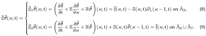
For the problem (8) and (9), the solution components and exhibit an initial layer at and interior layers at and , each of width . Furthermore, the solution component exhibits additional layers of width at , , and .
Proof.
The proof is by construction.
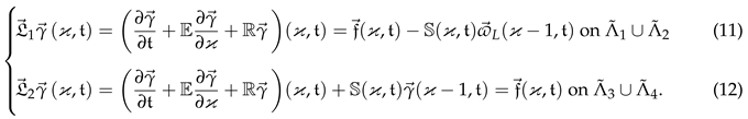
Case 1: Let be the particular solutions of
Consider the function
where and are solutions of
and , where are any particular vector constants. can be derived in the following way so as to have .
The product between vectors is the Schur product of vectors.
Case 2: Let be the particular solutions of
Consider the function
where and are solutions of
and , where be any particular vector constants. can be determined as follows to ensure that .
A similar approach confirms the existence of a solution for . When exists and is continuous at as is both well-defined and continuous at this point. The proof of the theorem is complete. □
2.1. Uniqueness and Stability Analysis
Continuous case
Lemma 1.
Proof. For , let us consider . If , there is nothing to prove. Let us assume that . Suppose then
which contradicts our assumption and for which also contradicts our assumption. Therefore . Also, and .
Thus, for , we have
which contradicts our assumption.
For , we get
which contradicts our assumption. If , then and there exists a neighborhood such that for all . If for any point , then . If for all , then we notice that is an increasing function in , as a consequence cannot attain its minimum at , which contradicts our assumption. This implies that and for all , then . The proof of the lemma is complete. □
Proof.
Consider the barrier functions
where
If , then
and
Lemma 1 implies that on . Then,
The proof of the lemma is complete. □
3. Solution Components and Layer Functions
The continuous solution of (1) is decomposed into .
The smooth component represents the solution of the following equation.
We have to deal with two different cases due to the presence of term in the domain.
Case 1:
 Case 2:
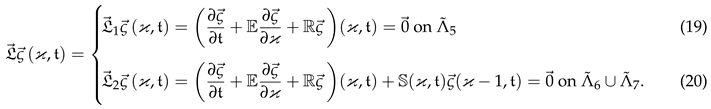
The singular component represents the solution of the following equation.
We have to deal with two different cases due to the presence of term in the domain.
Case 1:
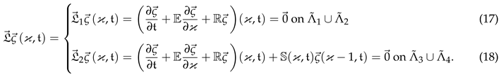
Case 2:
 with ,
We introduce , known as layer functions, which are associated with the solution as follows
where
4. Solution Bounds
Theorem 2.
Proof.
The bounds on the solutions are derived by employing steps and techniques analogous to those of Theorem 4.1 in [3]. □
The succeeding lemmas deal with finding bounds on and their derivatives.
Lemma 3.
Proof.
The bounds on the and its derivatives are derived by employing steps and techniques analogous to those of Lemma 5.1 in [3]. □
Lemma 4.
Case 1:For all and
Case 2:For all and
Proof.
The bounds on the and its derivatives are derived by employing steps and techniques analogous to those of Lemma 5.2 in [3]. □
4.1. Sharper Estimates
Definition 1.
For each , for Case 1 and for Case 2, the unique point in is defined by
Definition 2.
For all such that , there exist points that are uniquely defined and satisfy the inequalities presented below for Case 1 and Case 2.
Case 1:
Case 2:
Lemma 5.
for which the following estimates hold for each .
Case 1:For all and
Case 2:For all and
Proof.
The required estimates are derived by employing steps and techniques analogous to those of Lemma 10.3 in [3]. □
4.2. Domain Discretization
Temporal domain is meticulously discretized into a uniform mesh composed of mesh intervals on and . Now to capture the intricate layer behavior of the solutions, we discretized the spatial domain into a piecewise-uniform Shishkin mesh composed of mesh intervals and we have to deal with two different cases because of the presence of the discontinuous source term
For Case 1, the interval is partitioned into 12 sub-intervals, outlined as follows
The transition parameters are defined as:
The sub-intervals and are discretized using a uniform mesh consisting of mesh points. A uniform mesh consisting of mesh points is deployed on each of the sub-intervals and .
For Case 2, the interval is partitioned into 9 distinct sub-intervals, outlined as follows
The transition parameters are defined as:
The sub-intervals and are discretized using a uniform mesh consisting of mesh points. A uniform mesh consisting of mesh points is deployed on each of the sub-intervals and
The following symbols represent the key notation utilized throughout the text.
Case 1: Here , and
Case 2: Here and ,
Also, , , .
For the problem (1)–(3), we develop a classical layer resolving finite difference scheme using the aforementioned discretization.
The problem represented in (29) is reformulated for case 1 and case 2 is as follows:
Case 1:
Case 2:
where
for
Lemma 6.
Proof.
For , let and consider the case where the lemma does not hold. Then From the stipulated hypotheses, it is simple to establish that and
If , then
which is a contradiction. For , which leads to a contradiction.
Case 1: For
which contradicts our assumption. For we get
which contradicts our assumption.
Case 2: For
which contradicts our assumption. For we get
which contradicts our assumption.
If for case 1, then
Also,
and so
Then which contradicts our assumption.
If for case 2, then
Also,
and so
Then which contradicts our assumption. This implies that The proof of the lemma is complete. □
Lemma 7.
for and for Case 2,
for
Proof.
Define barrier functions
It is evident that on and also on on and for , we get
Hence, by the result of Lemma 6, we get on for Case 1. By applying analogous procedure used in Case 1, we get the required result on for Case 2. The proof of the lemma is complete. □
5. Discrete Solution Components and Error Estimates
The discrete solution of (29) are decomposed into , where and are discrete smooth and discrete singular components respectively.
The problem represented in (35) and (36) is reformulated for Case 1 and Case 2 are as follows:
Case 1:
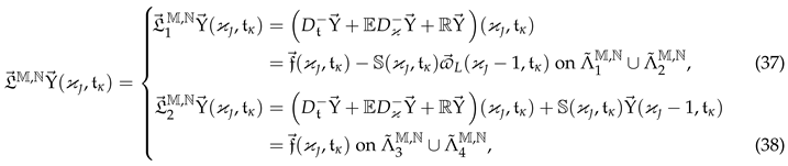
Case 2:
The error at each point is given by . For in Case 1 and in Case 2, the local truncation errors can be expressed as follows.
Theorem 3.
Let conditions (4) & (5) hold for and . Let represents the solution of (10) and let represents the solution of (35). Then, for Case 1
and for Case 2
Proof.
From the expressions (49) and (55), and using Lemma 3, for we get
The proof of the theorem is complete. □
Theorem 4.
Let conditions (4) & (5) hold for and . Let represents the solution of (16) and let represents the solution of (36). Then, for Case 1
and for Case 2
Proof.
The procedure outlined in Theorem 10.5 of [3] is employed in this theorem, as it leads to a similar result. □
From the above results, we concluded that for Case 1, or or and for Case 2, or ,
Now at the point or or for case 1 and or for case 2, we get
Theorem 5.
Proof.
For Case 1, consider the two mesh functions
and for Case 2,
where C is suitably chosen sufficiently large constant. Hence for Case 1, or or and for Case 2, or
and for Case 1, or or and for Case 2, or
For Case 1, or or and for Case 2, or
Thus, for N sufficiently large,
The proof of the theorem is complete. □
6. Numerical Illustration
To elucidate the proposed numerical scheme, an example is introduced in this section addresses two distinct cases resulting from the presence of discontinuous source term in the domain.
Example 1.
Case 1:Consider the following problem, where a discontinuity presents in the interval
where
and with
Case 2:Consider the following problem, where a discontinuity presents in the interval
where
and with
: maximum point-wise two-mesh differences,
: - uniform maximum point-wise two-mesh differences,
: - uniform order of local convergence,
: - uniform order of convergence and
: - uniform error constant.
and are computed using a variant of Two mesh algorithm [6] for both Case 1 & Case 2 of Example 1. The results are presented in Table 1 & Table 2.
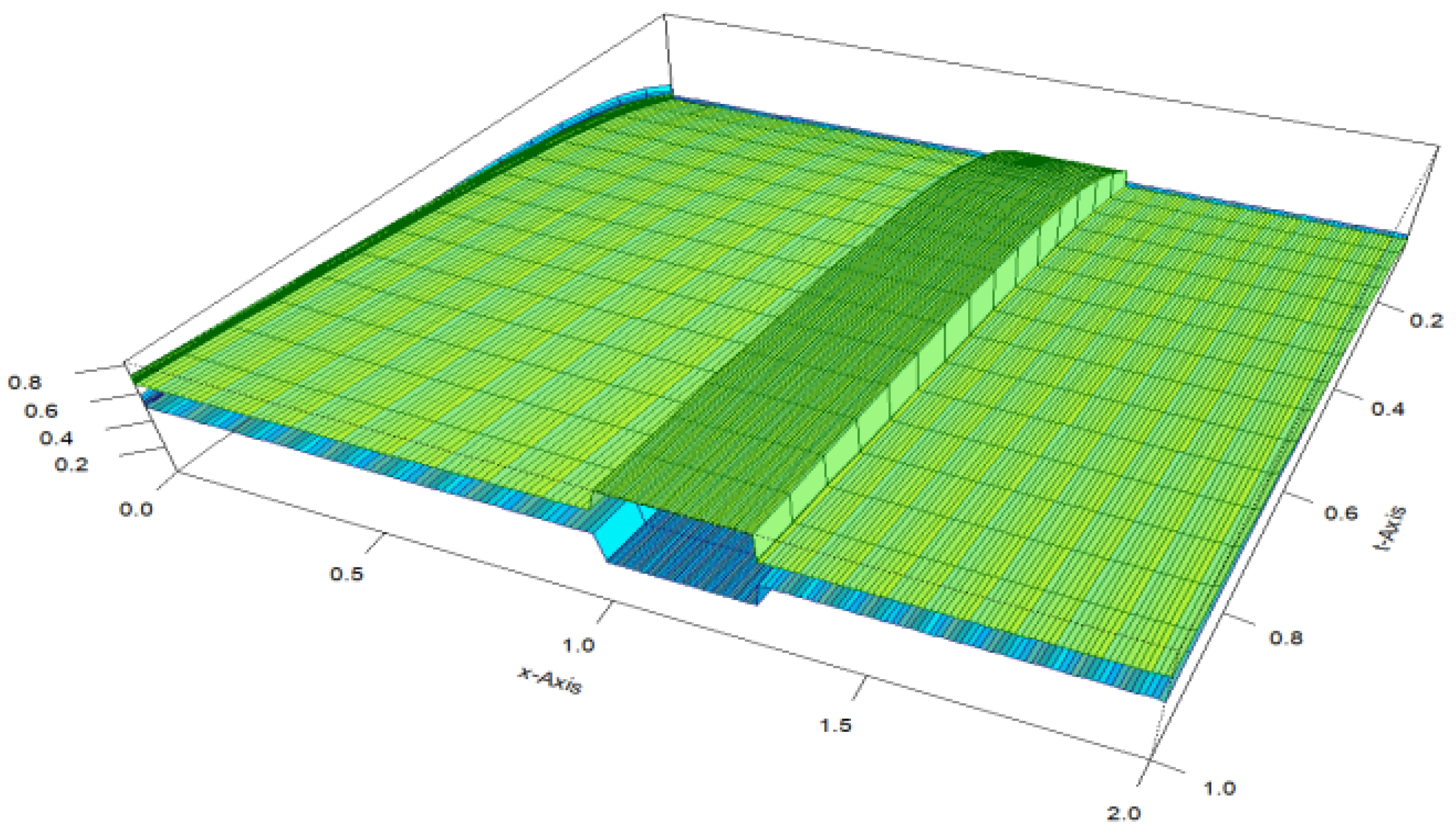
Figure 1.
Visualization of numerical solutions of Case 1 (Example 1), illustrating an initial layer at , and interior layers at , and .
Figure 1.
Visualization of numerical solutions of Case 1 (Example 1), illustrating an initial layer at , and interior layers at , and .
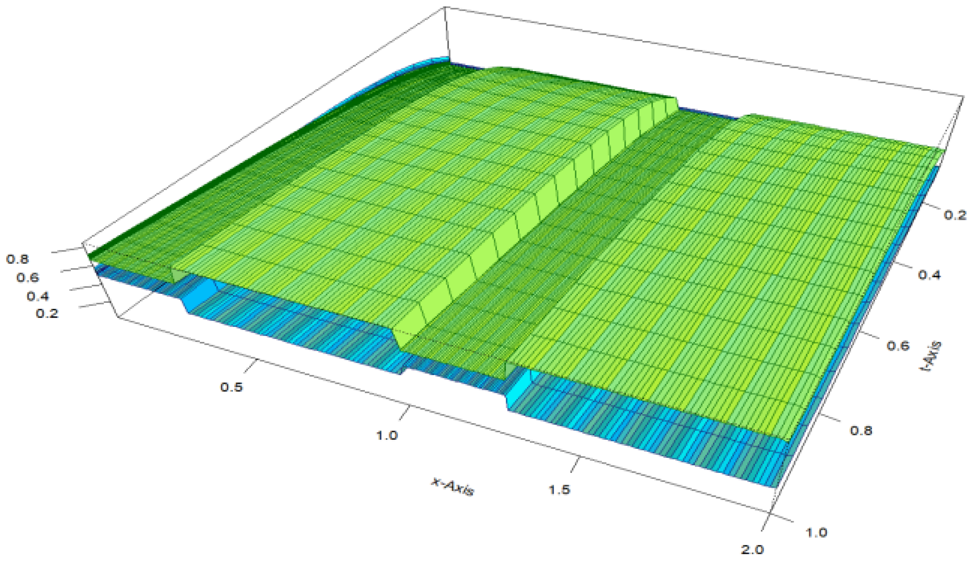
Figure 2.
Visualization of numerical solutions of Case 2 (Example 1), illustrating an initial layer at , and interior layers at and .
Figure 2.
Visualization of numerical solutions of Case 2 (Example 1), illustrating an initial layer at , and interior layers at and .
7. Conclusions
In this article, a classical layer resolving numerical scheme was constructed for solving a system of two time-dependent delay SPPs with a source term that exhibits a jump at a specific point due to discontinuity and robin initial conditions. This scheme incorporates a specially crafted piecewise uniform mesh to capture layer behaviors, formed in the initial and interior regions of the solution domain owing to the existence of delay and discontinuous source terms. Theoretical analysis and computational outcomes were validated through a numerical experiment, demonstrating strong concordance. Future research work will aim to solve semi-linear and nonlinear problems, with an emphasis on developing advanced numerical methods to improve computational efficiency.
References
- Abagero, B., Duressa, G., & Debela, H. (2021). Singularly perturbed Robin-type boundary value problems with discontinuous source term in geophysical fluid dynamics. Iranian Journal of Numerical Analysis and Optimization, 11(2), 351–364.
- Ajay Singh Rathore, & Vembu Shanthi. (2024). A numerical solution of singularly perturbed Fredholm integro-differential equation with discontinuous source term. Journal of Computational and Applied Mathematics, 446, 115858. [CrossRef]
- Bharathi, K. R., Chatzarakis, G. E., Panetsos, S. L., & Paramasivam, M. J. Robust Layer Resolving Scheme for a System of Two Singularly Perturbed Time-Dependent Delay Initial Value Problems with Robin Initial Conditions. (Accepted for publication in Australian Journal of Mathematical Analysis and Applications).
- Cen, Z., Huang, J., & Xu, A. (2023). A quadratic B-spline collocation method for a singularly perturbed semilinear reaction–diffusion problem with discontinuous source term. Mediterranean Journal of Mathematics, 20, 269. [CrossRef]
- Chawla, S., Urmil, & Singh, J. (2021). A parameter-robust convergence scheme for a coupled system of singularly perturbed first-order differential equations with discontinuous source term. International Journal of Applied and Computational Mathematics, 7, 118. [CrossRef]
- Farrell, P., Hegarty, A., Miller, J. M., O’Riordan, E., & Shishkin, G. I. (2000). Robust computational techniques for boundary layers. Chapman and Hall/CRC.
- Paramasivam, M., Miller, J. J. H., & Valarmathi, S. (2014). Parameter-uniform convergence for a finite difference method for a singularly perturbed linear reaction-diffusion system with discontinuous source terms. International Journal of Numerical Analysis and Modeling, 11(2), 385–399.
- Sahoo, S. K., & Gupta, V. (2022). Higher-order robust numerical computation for singularly perturbed problems involving discontinuous convective and source terms. Mathematical Methods in the Applied Sciences, 45(8), 4876–4898. [CrossRef]
- Selvaraj, D., & Mathiyazhagan, J. P. (2021). A parameter-uniform convergence for a system of two singularly perturbed initial value problems with different perturbation parameters and Robin initial conditions. Malaya Journal of Matematik, 9(1), 498–505. [CrossRef]
- Singh, S., Choudhary, R., & Kumar, D. (2023). An efficient numerical technique for two-parameter singularly perturbed problems having discontinuity in convection coefficient and source term. Computational and Applied Mathematics, 42(62). [CrossRef]
- Soundararajan, R., Subburayan, V., & Wong, P. J. Y. (2023). Streamline diffusion finite element method for singularly perturbed 1D-parabolic convection-diffusion differential equations with line discontinuous source. Mathematics, 11(9), 2034. [CrossRef]

Table 1.
For Case 1, Values of and generated for
| ℷ | : Number of mesh points | |||
|---|---|---|---|---|
| 96 | 192 | 384 | 768 | |
| 0.100E-01 | 0.106E+00 | 0.673E-01 | 0.406E-01 | 0.236E-01 |
| 0.100E-03 | 0.106E+00 | 0.673E-01 | 0.406E-01 | 0.236E-01 |
| 0.100E-05 | 0.106E+00 | 0.673E-01 | 0.406E-01 | 0.236E-01 |
| 0.100E-07 | 0.106E+00 | 0.673E-01 | 0.406E-01 | 0.236E-01 |
| 0.100E-09 | 0.106E+00 | 0.673E-01 | 0.406E-01 | 0.236E-01 |
| 0.106E+00 | 0.673E-01 | 0.406E-01 | 0.236E-01 | |
| 0.655E+00 | 0.730E+00 | 0.782E+00 | ||
| 0.577E+01 | 0.577E+01 | 0.548E+01 | 0.501E+01 | |
Table 2.
For Case 2, Values of and generated for
| ℷ | : Number of mesh points | |||
|---|---|---|---|---|
| 144 | 288 | 576 | 1152 | |
| 0.100E-01 | 0.634E-01 | 0.385E-01 | 0.225E-01 | 0.128E-01 |
| 0.100E-03 | 0.634E-01 | 0.385E-01 | 0.225E-01 | 0.128E-01 |
| 0.100E-05 | 0.634E-01 | 0.385E-01 | 0.225E-01 | 0.128E-01 |
| 0.100E-07 | 0.634E-01 | 0.385E-01 | 0.225E-01 | 0.128E-01 |
| 0.100E-09 | 0.634E-01 | 0.385E-01 | 0.225E-01 | 0.128E-01 |
| 0.634E-01 | 0.385E-01 | 0.225E-01 | 0.128E-01 | |
| 0.721E+00 | 0.774E+00 | 0.812E+00 | ||
| 0.579E+01 | 0.579E+01 | 0.558E+01 | 0.524E+01 | |
Disclaimer/Publisher’s Note: The statements, opinions and data contained in all publications are solely those of the individual author(s) and contributor(s) and not of MDPI and/or the editor(s). MDPI and/or the editor(s) disclaim responsibility for any injury to people or property resulting from any ideas, methods, instructions or products referred to in the content. |
© 2025 by the authors. Licensee MDPI, Basel, Switzerland. This article is an open access article distributed under the terms and conditions of the Creative Commons Attribution (CC BY) license (http://creativecommons.org/licenses/by/4.0/).
Copyright: This open access article is published under a Creative Commons CC BY 4.0 license, which permit the free download, distribution, and reuse, provided that the author and preprint are cited in any reuse.


