AFAR-WQS: A Quick and Simple Toolbox for Water Quality Simulation

Carlos Andrés Rogéliz-Prada; Jonathan Nogales

doi:10.20944/preprints202501.1158.v1

Submitted:

15 January 2025

Posted:

15 January 2025

You are already at the latest version

Abstract

Effective water quality management in large-scale river networks is critical for maintaining ecosystem health and ensuring sustainable water resources. Given the complexities of developing detailed water quality models at the macro-watershed scale, there is an increasing need for preliminary approaches that provide rapid, practical insights, especially in data-limited or resource-constrained contexts. This paper presents AFAR-WQS (Assimilation Factor Analysis of Rivers for Water Quality Simulation), a MATLAB-based tool designed to simulate 13 key water quality determinants using the steady-state assimilation factors framework. The tool integrates graph theory and a Depth-First Search (DFS) algorithm to model assimilation factors, concentrations, and loads for each water quality determinant, incorporating both diffuse and point-source pollution. AFAR-WQS enables large-scale simulations with minimal computational demands and low data requirements, providing researchers, managers, and policymakers with an accessible tool for optimizing intervention strategies and resource allocation in river basin management. The DFS algorithm employed by AFAR-WQS demonstrates efficient computational performance, resolving river networks with up to 100,000 segments within minutes, making it well-suited for macro-basin scale applications.

Keywords:

Water quality modeling

;

River basin management

;

Matlab toolbox

;

Assimilation factor

Subject:

Environmental and Earth Sciences - Environmental Science

1. Introduction

The analysis and understanding of water systems in large basins present significant challenges in the development of tools that enable a multidimensional understanding of the current state of natural resources and the impacts that may arise from specific actions within a basin. A comprehensive view of water systems requires not only an understanding of water quantity but also water quality [1,2,3,4], which is a crucial parameter for assessing the health of freshwater ecosystems and their potential for sustainable use [5].

According to [6], approximately 80% of global industrial and municipal wastewater is discharged into the environment without prior treatment. This percentage is even higher in less developed countries, where the lack of infrastructure for sanitation and wastewater treatment is more severe. This situation has significant negative repercussions, not only for human health but also for the functioning of aquatic ecosystems and socio-economic development [6,7]. Moreover, the continuous growth of the global population, along with increased freshwater consumption for human use, agriculture, and industry, amplifies these challenges [8].

One of the most useful tools for understanding water quality is mathematical modeling [9]. Currently, the range of available models that allow us to understand water quality dynamics in watersheds is quite diverse. Some of the models cited in the literature include Agricultural Non-Point Source, AGWA, ANSWERS-2000, APEX, AQUATOX, BASINS, EFDC, EPD-RIV1, GLEAMS/CREAMS, HSPF, InVEST, KINEROS2, LSPC, MIKE SHE, NLEAP, PRMS, QUAL2E, QUAL2K, SIGA-CAL, SWAT, SWMM, WAM, WARMF, WASP7, WCS, AquaChem, TOMCAT, SisBaHIA, SIMCAT, QUAL2KW, MOHID, MIKE HYDRO, and CE-QUAL-W2 [4,10]. Each of these models has advantages and disadvantages, and various studies have focused on comparing them [5,11].

In the management of water systems, decision-making at the macro-basin level often requires a preliminary understanding to quickly guide decisions, such as resource allocation or evaluating the feasibility of a request [12]. However, a common denominator among many of the mentioned models is that their complexity, computational demand, and information requirements for implementation and calibration pose significant challenges for their practical application at the macro-basin scale [13].

In this context, the need for preliminary approaches that facilitate more detailed and robust analyses is clear. This requires the implementation of computationally efficient tools that can provide approximate results quickly. One example of such tools is the InVEST models [14], which are designed to support natural resource management, particularly in implementing nature-based solutions. There are cases, such as SWAT, which has been integrated into the Hydrologic and Water Quality System (HAWQS), a national-scale decision support system (DSS) that allows for simple and intuitive modeling of large watersheds [15]. Similarly, InVEST has been incorporated into WaterProof, a web-based decision support tool that provides quick calculations of return on investment (ROI) and early indications of an optimal portfolio of nature-based solutions (NBS) for any watershed globally [16]. However, while the use of such platforms should be encouraged, they still present limitations for global-scale basin analysis. These limitations include longer calculation times, complex preliminary configurations before the model becomes operational on the platform, and default configurations based on global databases that do not adequately capture the local characteristics of the territory.

Given this situation, there is a significant gap in water quality modeling innovation, particularly in designing efficient algorithms and computational procedures to approximate system behavior. Recently, [17] presented a simplified water quality model based on the concept of assimilation factors [18,19] for 13 water quality determinants: temperature (T), organic nitrogen (NO), ammoniacal nitrogen (NH₄), nitrates (NO₃), organic phosphorus (Po), inorganic phosphorus (Pi), organic matter (OM), dissolved oxygen (DO), suspended solids (SS), pathogenic organisms (X), elemental mercury (Hg0), divalent mercury (Hg2), and methylmercury (MeHg). This parsimonious approach has been used to identify priorities in sanitation [20,21,22,23], national-scale water resource management [22], and as an approximation of the health and integrity of freshwater ecosystems [17,24].

In this research, we present a computational implementation of the model proposed by [17]. The implementation is carried out as an open-source MATLAB™ toolbox called AFAR-WQS (Assimilation Factor Analysis of Rivers for Water Quality Simulation). This toolbox employs a Depth-First Search (DFS) algorithm to efficiently resolve cumulative processes in complex topological networks, maximizing computational performance. AFAR-WQS simulates the concentration, loads, and assimilation factors of the 13 water quality determinants. Additionally, it allows for the integration of diffuse sources of pollution by basin, point discharges, and boundary conditions. The toolbox was developed using an object-oriented programming approach, which facilitates scalability and maintenance. Furthermore, it incorporates an interactive user interface that enables visual analysis of the model results, allowing users to explore variations in water quality conditions from the reach to the network scale, thus facilitating interpretation and decision-making in water resource management.

2. Materials and Methods

AFAR-WQS was developed using the concept of assimilation factors to model the 13 water quality parameters it evaluates. Conceptually, this factor is defined as the stream's capacity to absorb and mitigate the impact of a contamination event [18,19]. According to [18,19], this concept is intrinsically linked to the physical, chemical, and biological processes that influence the contaminant within the receiving water body. Mathematically, the assimilation factor is expressed as:

a = \frac{W_{u}}{C}

where

a

represents the assimilation factor, which depends on the characteristics of the receiving water body and the nature of the contaminant;

W_{u}

corresponds to the pollutant load originating from upstream segments (with the subscript

u

indicating the concentration of the parameter at that point); and

C

denotes the downstream concentration in the segment.

Operationally, AFAR-WQS represents the drainage network of a watershed as a directed graph, allowing each river segment to be modeled as a connection between two nodes, as illustrated in Figure 1a. Using this framework, AFAR-WQS resolves the topological connectivity of the network through a Depth-First Search (DFS) algorithm [25], which begins at the segment corresponding to the watershed outlet. From this point, the algorithm progresses upstream through the drainage network until it identifies a headwater segment, defined as one with no incoming connections. (Figure 1b). Upon identifying a headwater segment, the model begins aggregating loads for various water quality determinants, estimating both assimilation factors and concentrations for that specific reach (Figure 1c). The algorithm then proceeds downstream to the immediately adjacent reach. If this downstream reach has incoming connections, the model recursively moves upstream, repeating the process described until it returns to the original confluence point. Figure 1c illustrates the manner in which concentrations are estimated for intermediate and headwater reaches.

This modeling scheme assumes that the physicochemical conditions are uniform throughout the entire reach, as it represents the smallest modeling unit in AFAR-WQS. Therefore, the assimilation factors are calculated based on the average values of the physicochemical characteristics of the reach. Moreover, the recursive approach used by the tool to solve the topological network allows for the analysis of networks with a large number of nodes while using minimal storage resources, a capability that would not be possible with adjacency matrix-based schemes, which require significantly higher computational resources [26].

Reach segmentation can be performed automatically, either based on an area accumulation threshold or a maximum length defined by the user, employing tools such as Topotoolbox [27], ArcHydro [28], and ArcSWAT [29], which facilitate the generation of river networks from a digital elevation model (DEM). AFAR-WQS offers the advantage of resolving connections involving more than two reaches connected to a node, as well as one-to-one reach connections. However, it is important to note that the tool cannot represent cyclic connections or bifurcations within the network. Additionally, it assumes that the graph is unidirectional, with connections directed toward the reach representing the basin's outlet. This flexibility allows the topological network to be segmented at points of interest defined by the user. AFAR-WQS also supports the representation of topological networks with multiple outlets, which is particularly relevant in decision-making processes where boundaries are guided not strictly by watershed divides but by political or administrative limits.

Toolbox Configuration

The configuration of AFAR-WQS requires assigning each reach in the network a set of physical attributes related to the geomorphological characteristics of the river reaches to be modeled, which govern the transport conditions of the water quality determinants (see Table 1). All the necessary attributes for the tool can be derived from mathematical models (e.g. hydrological, hydrodynamic, etc.), prior studies, field data, or a combination of these sources. However, AFAR-WQS estimates certain key parameters by default, such as average travel time, dispersive fraction, advection time, and residence time. Given that the tool is developed using an object-oriented programming approach, users can customize it by incorporating additional methods tailored to their specific study area, allowing for the estimation of other attributes required by the tool.

Depending on the water quality determinant to be modeled, it is necessary to assign the corresponding reaction rates and decay parameters (see Table 2). By default, the tool incorporates the values used by [17] for all determinants. However, these parameters are fully editable by the user, allowing for greater flexibility to adapt the model to the specific conditions of the study area.

3. Results and Discussion

3.1. Toolbox Structure

The file and folder structure used by the toolbox is illustrated in Figure 2. The @ClassNetwork object represents the topological network and includes the recursive accumulation operations across this network. In turn, @AFAR_WQS groups the necessary methods for estimating the concentrations and assimilation factors of the various water quality determinants, inheriting the properties and methods of @ClassNetwork. Each determinant is modeled as a specific method within the @AFAR_WQS object, and these methods are executed independently. This allows the user to configure only the required inputs for the specific water quality determinant they intend to model.

AFAR-WQS takes the drainage network as input, organized in a data structure called ReachData. Each row in ReachData corresponds to an individual reach in the network, while the columns contain the geomorphological and physicochemical characteristics of the reach (detailed in Table 1). The ReachData structure can be exported as a shapefile, allowing for visualization and further analysis in any Geographic Information System (GIS) software.

As for the outputs, the toolbox calculates the concentration for each water quality determinant (expressed in mg/L for most determinants, except for coliforms, which is expressed in MPN/L), the assimilation factors in liters, and the loads in mg/day (except for coliforms, which is expressed in MPN/day). These results correspond to the flow scenario previously configured by the user. If different flow conditions need to be evaluated, the user can run multiple model executions to represent various discharge scenarios.

3.2. Computational Performance

The DFS algorithm [25] employed by AFAR-WQS to resolve the topological connectivity of the network exhibits strong computational performance, delivering results within minutes. On a computer equipped with an Intel(R) Core(TM) i7-10750H CPU @ 2.60GHz and 64.0 GB of RAM, AFAR-WQS completes the modeling of a single water quality parameter for a network comprising 30,000 river segments in just 163 seconds (see Figure 3). A key advantage of AFAR-WQS is its low memory usage, as it does not generate vector data structures larger than the total number of segments in the network. Notably, due to the recursive nature of the DFS algorithm, the computational time scales following a power-law relationship as the number of segments increases. However, for networks containing up to 100,000 segments, the computation times remain manageable and aligned with the requirements of macro-basin scale modeling. The implementation of AFAR-WQS was validated using the results from [17], where we verified that the approach accurately reproduces the original outcomes.

3.3. Outputs and Visualization Options

When modeling a water quality determinant with AFAR-WQS, three key outputs are generated: 1) the concentration of the water quality determinant at the outlet of each reach (represented by object variables starting with “C_”), 2) the assimilation factor for the water quality determinant within the reach (represented by variables beginning with “AF_”), and 3) the load of the water quality determinant at the reach outlet (represented by variables beginning with “W_”). These outputs are generated for each reach in the analysis network and are stored as column vectors within the object representing the network, thereby facilitating efficient data management and analysis.

The toolbox also provides a Matlab application developed in App Designer, enabling users to visualize the results of each water quality determinant and support model interpretation. In the application interface, users can select both the variable and the water quality determinant they wish to visualize (see Figure 4a). The tool offers two visualization options: a network-level representation and a longitudinal profile. For the longitudinal profile, users must specify the ReachID of the initial reach for the determinant profile. In this visualization, the graph displays the cumulative reach distance on the horizontal axis, spanning from the selected starting reach to the network outlet (river mouth), while the vertical axis illustrates changes in the analyzed determinant variable along the profile (see Figure 4b).

Additionally, the Matlab application allows users to customize the color palette used to visualize the water quality determinant variable, thereby improving visual comprehension and facilitating the analysis of model results.

4. Conclusions

The AFAR-WQS toolbox has been developed to facilitate access to and use of the model presented by [17], a computationally efficient, parsimonious, and flexible approach for conducting network-scale water quality assessments based on assimilation factors. Its flexibility allows configuration using both primary and secondary data, enhancing its versatility and adaptability to various informational needs, geographic regions, and specific study requirements. Moreover, its computational efficiency ensures that large and complex networks can be analyzed within reasonable timeframes, even on standard hardware.

The AFAR-WQS toolbox is supported by a comprehensive codebase and documentation, complemented by a detailed user guide that facilitates its implementation and use. It is designed for seamless data exchange between Matlab and GIS environments, streamlining data preparation, information sharing, and result visualization. We encourage researchers and the broader community to widely adopt AFAR-WQS widely and contribute to its development by adding new assimilation factors for water quality determinants or enhancing existing ones. We hope that the use of and contributions to AFAR-WQS will improve the management and decision-making related to water quality in freshwater ecosystems. The AFAR-WQS toolbox and user documentation are available for free at the GitHub repository (https://github.com/N4W-Facility/AFAR-WQS_Toolbox).

Author Contributions

Conceptualization, C.A.R.-P. and J.N.; methodology, C.A.R.-P. and J.N.; software, J.N.; validation, C.A.R.-P.; writing—original draft preparation, J.N.; writing—review and editing, C.A.R.-P.; visualization, C.A.R.-P. and J.N.; supervision, C.A.R.-P.; project administration, C.A.R.-P.; funding acquisition, C.A.R.-P. All authors have read and agreed to the published version of the manuscript.

Funding

This research was funded by Nature for Water Facility.

Software Availability

Name of software: AFAR-WQS toolbox. Version: 1.0 tested on Matlab R2023b. Developers: Jonathan Nogales, Carlos A. Rogéliz. Contact email: carlos.rogeliz@tnc.org. Year first available: 2024. Available from: GitHub repository (https://github.com/N4W-Facility/AFAR-WQS_Toolbox).

Acknowledgments

The authors extend their sincere gratitude to the Nature for Water Facility for its invaluable support in fostering and advancing this research, as well as for its unwavering commitment to the advancement of scientific knowledge and the implementation of nature-based solutions.

Conflicts of Interest

The authors declare no conflicts of interest.

References

Tao, Y.; Tao, Q.; Qiu, J.; Pueppke, S.G.; Gao, G.; Ou, W. Integrating Water Quantity- and Quality-Related Ecosystem Services into Water Scarcity Assessment: A Multi-Scenario Analysis in the Taihu Basin of China. Applied Geography 2023, 160, 103101. [CrossRef]
Hwang, J.H.; Park, S.H.; Song, C.M. A Study on an Integrated Water Quantity and Water Quality Evaluation Method for the Implementation of Integrated Water Resource Management Policies in the Republic of Korea. Water (Basel) 2020, 12, 2346. [CrossRef]
Nowicki, S.; Koehler, J.; Charles, K.J. Including Water Quality Monitoring in Rural Water Services: Why Safe Water Requires Challenging the Quantity versus Quality Dichotomy. NPJ Clean Water 2020, 3, 14. [CrossRef]
Jiménez, M.; Usma, C.; Posada, D.; Ramírez, J.; Rogéliz, C.A.; Nogales, J.; Spiro-Larrea, E. Planning and Evaluating Nature-Based Solutions for Watershed Investment Programs with a SMART Perspective Using a Distributed Modeling Tool. Water (Basel) 2023, 15, 3388.
Talukdar, P.; Kumar, B.; Kulkarni, V. V. A Review of Water Quality Models and Monitoring Methods for Capabilities of Pollutant Source Identification, Classification, and Transport Simulation. Rev Environ Sci Biotechnol 2023, 22, 653–677. [CrossRef]
Dr. Amit Krishan; Dr. Shweta Yadav; Ankita Srivastava Water Pollution’s Global Threat to Public Health : A Mini-Review. Int J Sci Res Sci Eng Technol 2023, 321–334. [CrossRef]
du Plessis, A. Persistent Degradation: Global Water Quality Challenges and Required Actions. One Earth 2022, 5, 129–131. [CrossRef]
Rajak, P.; Ganguly, A.; Nanda, S.; Mandi, M.; Ghanty, S.; Das, K.; Biswas, G.; Sarkar, S. Toxic Contaminants and Their Impacts on Aquatic Ecology and Habitats. In Spatial Modeling of Environmental Pollution and Ecological Risk; Elsevier, 2024; pp. 255–273.
Benedini, M.; Tsakiris, G. Water Quality Modelling for Rivers and Streams; Springer Netherlands: Dordrecht, 2013; Vol. 70; ISBN 978-94-007-5508-6.
Ejigu, M.T. Overview of Water Quality Modeling. Cogent Eng 2021, 8. [CrossRef]
Darji, J.; Lodha, P.; Tyagi, S. Assimilative Capacity and Water Quality Modeling of Rivers: A Review. Journal of Water Supply: Research and Technology-Aqua 2022, 71, 1127–1147. [CrossRef]
Beven, K. How to Make Advances in Hydrological Modelling. Hydrology Research 2019, 50, 1481–1494. [CrossRef]
Hofstra, N.; Kroeze, C.; Flörke, M.; van Vliet, M.T. Editorial Overview: Water Quality: A New Challenge for Global Scale Model Development and Application. Curr Opin Environ Sustain 2019, 36, A1–A5. [CrossRef]
Natural Capital Project InVEST 3.13.0.Post6+ug.G6b07b42 User’s Guide.; 2022;
Yen, H.; Daggupati, P.; White, M.; Srinivasan, R.; Gossel, A.; Wells, D.; Arnold, J. Application of Large-Scale, Multi-Resolution Watershed Modeling Framework Using the Hydrologic and Water Quality System (HAWQS). Water (Basel) 2016, 8, 164. [CrossRef]
Rogéliz, C.A.; Vigerstol, K.; Galindo, P.; Nogales, J.; Raepple, J.; Delgado, J.; Piragauta, E.; González, L. WaterProof—A Web-Based System to Provide Rapid ROI Calculation and Early Indication of a Preferred Portfolio of Nature-Based Solutions in Watersheds. Water (Basel) 2022, 14, 3447.
Nogales, J.; Rogéliz-Prada, C.; Cañon, M.A.; Vargas-Luna, A. An Integrated Methodological Framework for the Durable Conservation of Freshwater Ecosystems: A Case Study in Colombia’s Caquetá River Basin. Front Environ Sci 2023, 11, 1264392. [CrossRef]
Chapra, S.C. Surface Water-Quality Modeling; 15th ed.; Waveland press: Illinois, 2008;
Chapra, S.C. Surface Water Quality Modelling. Mc Graw Hill. ; 1997;
Rojas, A. Aplicación de Factores de Asimilación Para La Priorización de La Inversión En Sistemas de Saneamiento Hídrico En Colombia. Thesis, Universidad Nacional de Colombia: Bogotá D.C., 2011.
Navas, A. Factores de Asimilación de Carga Contaminante En Ríos - Una Herramienta Para La Identificación de Estrategias de Saneamiento Hídrico En Países En Desarrollo, 2016.
Mamani, J.A. Desarrollo de Un Modelo Numérico de Calidad Del Agua En Un Marco Probabilístico de Soporte a Las Decisiones a Escala Nacional. Thesis, Univerdad de los Andes: Bogotá D.C, 2022.
Correa-Caselles, D. Metodología Para La Estimación Del Destino y Transporte de Mercurio Presente En Los Ríos de Colombia. Thesis, Univerdad de los Andes: Bogotá D.C, 2022.
Rivera Gutiérrez, J.V. Evaluation of the Kinetics of Oxidation and Removal of Organic Matter in the Self-Purification of a Mountain River. Dyna (Medellin) 2015, 82, 183–193. [CrossRef]
Hopcroft, J.; Tarjan, R. Algorithm 447: Efficient Algorithms for Graph Manipulation. Commun ACM 1973, 16, 372–378. [CrossRef]
Tangi, M.; Schmitt, R.; Bizzi, S.; Castelletti, A. The CASCADE Toolbox for Analyzing River Sediment Connectivity and Management. Environmental Modelling & Software 2019, 119, 400–406. [CrossRef]
Schwanghart, W.; Scherler, D. Short Communication: TopoToolbox 2 – MATLAB-Based Software for Topographic Analysis and Modeling in Earth Surface Sciences. Earth Surface Dynamics 2014, 2, 1–7. [CrossRef]
ESRI, M.D. ArcHydro: GIS for Water Resources 2013.
Winchell, M.; Srinivasan, R.; Di Luzio, M.; Arnold, J.G. ArcSWAT 2.3. 4 Interface For SWAT2005. Grassland, soil and research service, Temple, TX 2009.
Flores, A.N.; Bledsoe, B.P.; Cuhaciyan, C.O.; Wohl, E.E. Channel-reach Morphology Dependence on Energy, Scale, and Hydroclimatic Processes with Implications for Prediction Using Geospatial Data. Water Resour Res 2006, 42, 6412. [CrossRef]
Wohl, E.; Merritt, D. Prediction of Mountain Stream Morphology. Water Resour Res 2005, 41. [CrossRef]
González, R. Determinación Del Comportamiento de La Fracción Dispersiva En Ríos Característicos de Montaña, UNAL: Bogotá D.C. , 2008.
Schmitt, R.J.P.; Bizzi, S.; Castelletti, A. Tracking Multiple Sediment Cascades at the River Network Scale Identifies Controls and Emerging Patterns of Sediment Connectivity. Water Resour Res 2016, 52, 3941–3965. [CrossRef]
Wilkerson, G. V.; Parker, G. Physical Basis for Quasi-Universal Relationships Describing Bankfull Hydraulic Geometry of Sand-Bed Rivers. Journal of Hydraulic Engineering 2011, 137, 739–753. [CrossRef]
Parker, G.; Wilcock, P.R.; Paola, C.; Dietrich, W.E.; Pitlick, J. Physical Basis for Quasi-Universal Relations Describing Bankfull Hydraulic Geometry of Single-Thread Gravel Bed Rivers. J Geophys Res Earth Surf 2007, 112. [CrossRef]

Figure 1. (a) Graph representation of a synthetic drainage network with seven reaches. (b) Schematic of the recursive solution framework used by AFAR-WQS to estimate assimilation factors and concentrations across the drainage network. (c) Example calculation of the concentration of a determinant j for a synthetic network with seven reaches.

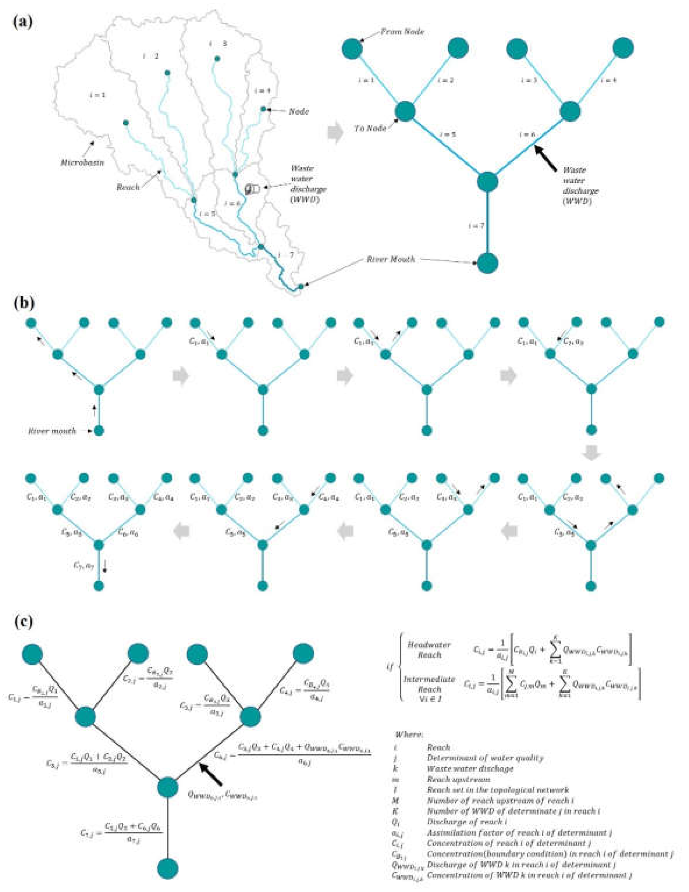
Figure 2. Folder structure and functions of the AFAR-WQS Toolbox.

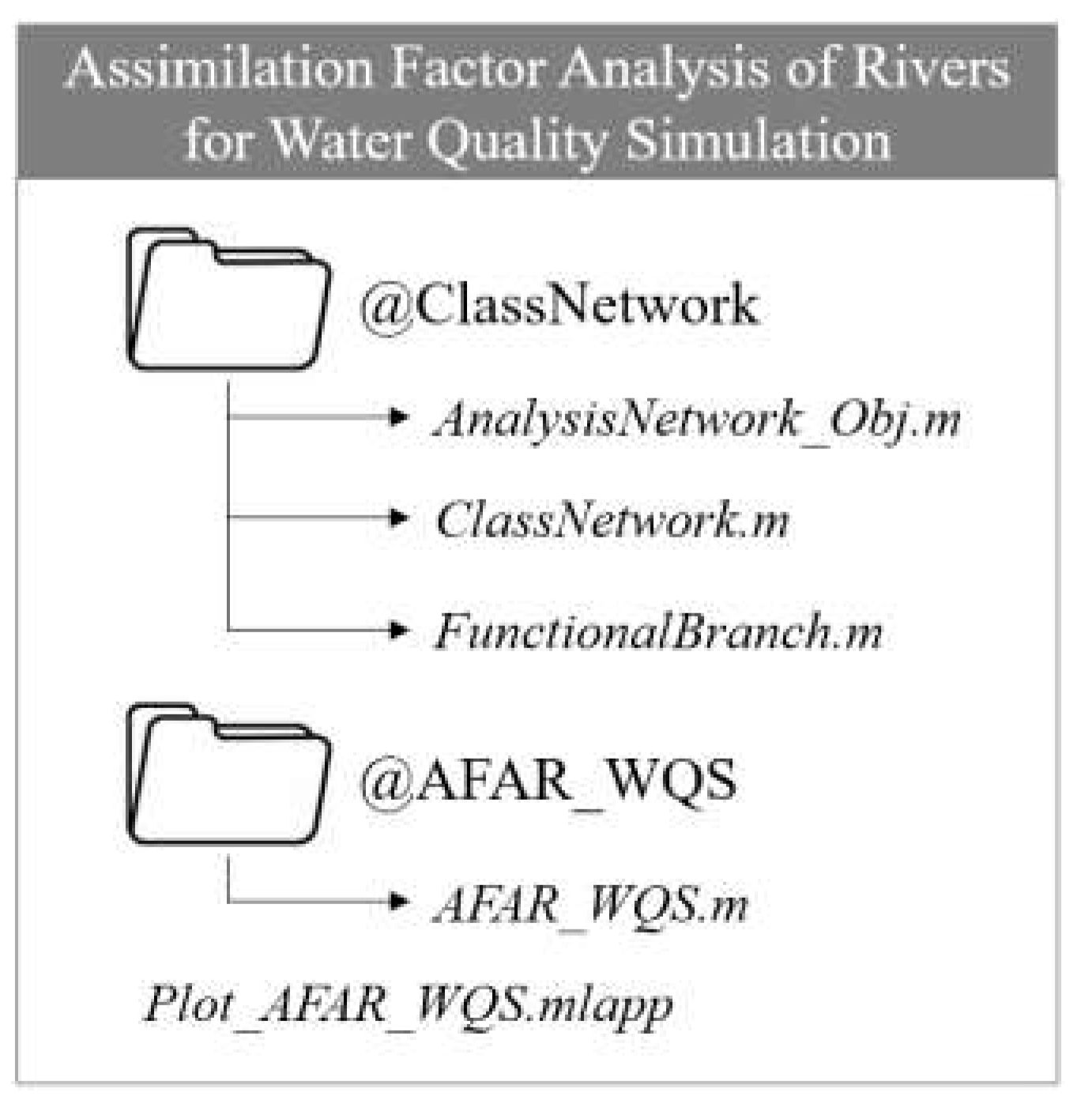
Figure 3. AFAR-WQS computational performance by number of drainage network segments

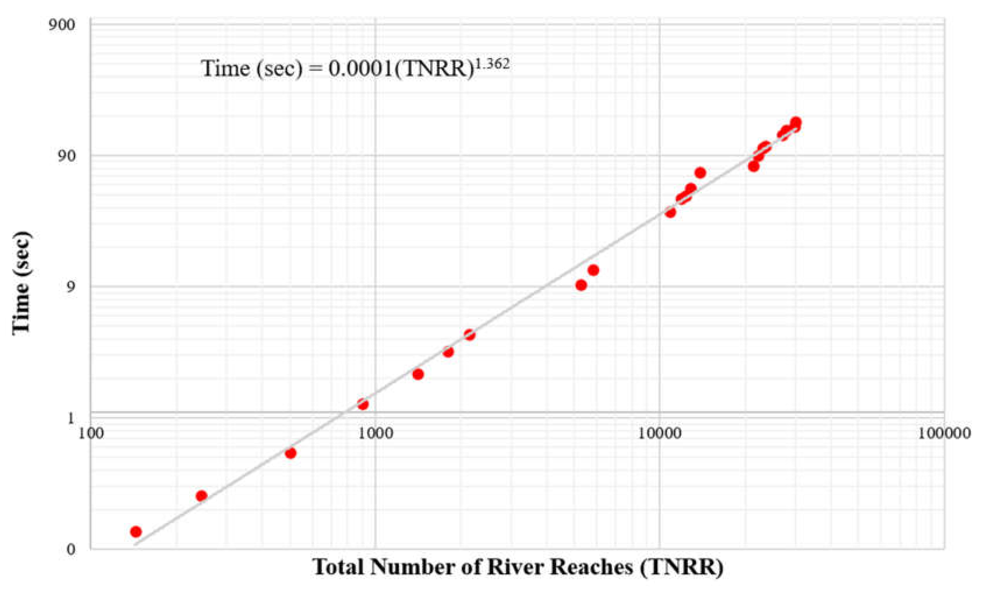
Figure 4. Visualization examples of suspended solids for a synthetic network. (a) illustrates the network-wide distribution of suspended solids concentration. (b) depicts the suspended solids profile extending from reach 929 to the network outlet.

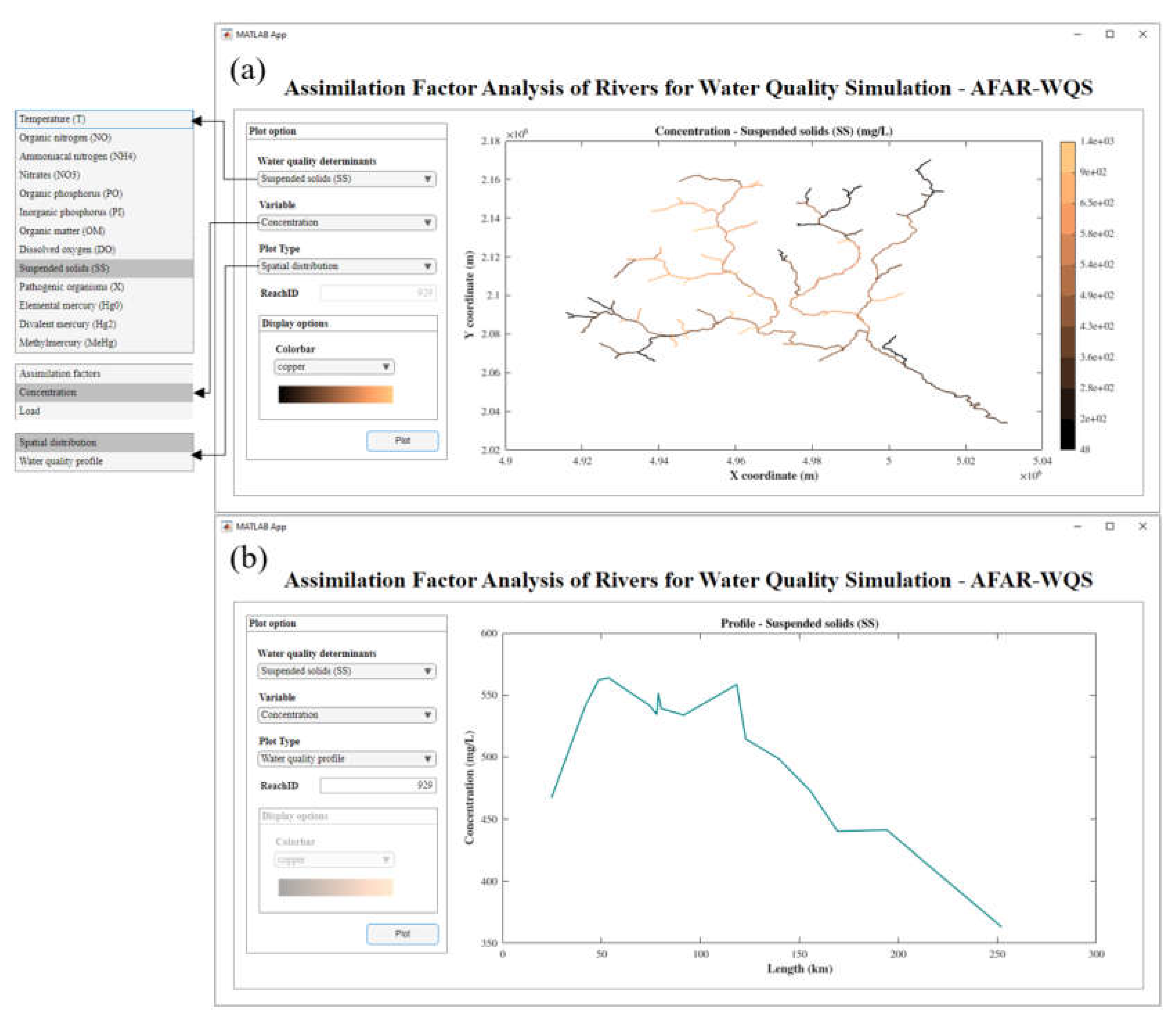
Table 1. Attributes that are assigned to each topological network reach.

Attributes	Unit	Description
ReachID	-	Unique positive integer numeric identifier of each reach in the topological network
FromNode	-	Positive integer numeric identifier of the initial node of a reach of the topological network.
ToNode	-	Positive integer numerical identifier of the end node of a reach of the topological network.
ReachType	-	Identifies whether the reach represents a plain or mountain river. If false is specified, the tool will assume that the reach represents a plain river. To define whether a river is a plain or a mountain river, a first criterion may be to assume that the former is limited by capacity (slope ≤0.025 m/m) and the latter by supply (slope >0.025 m/m), this, following the slope thresholds defined by [30]. A second criterion may be to use the slope threshold defined by [31] to define whether a river is mountain (slope >0.002 m/m) or plain (slope <0.002 m/m).
RiverMouth	-	Identifies the river reach that corresponds to the basin closure point. If the value is false, it is considered not to be a closure point reach.
$D F$ ^**	dimensionless	The tool estimates the dispersive fraction following the criteria of [32]. For the sections of the topological network representing mountain rivers, an overall value of 0.27 is considered, while for plain rivers it is 0.40.
$\bar{t}$	day	$The tool estimates the average travel time as : U_{s} = \frac{U}{1 + β} \bar{t} = (\frac{L}{U_{s}}) * (\frac{1}{3600 * 24})$ $Where U_{s}$ is solute velocity (m/s); β is the effective delay coefficient. According to [32] the effective delay coefficient for mountain rivers has an overall magnitude of 1.10 while for plain rivers it is 2.0.
$τ$ ^**	day	$The tool estimates the advection time as : τ = \bar{t} * (1 - D F)$
$T R$ ^**	day	$The tool estimates the residence time as : T R = \bar{t} * D F$
L	m	River length representing the reach in the topological network
Z	m.a.s.l	Average elevation of the river representing the reach in the topological network
A	m²	Drainage area of the river representing the reach in the topological network, accumulated up to the ToNode of the reach
Q	m³/s	Average discharge of the river representing the reach in the topological network, for a selected discharge scenario
W	m	Average width of the river's cross-section representing the reach in the topological network, for the selected discharge scenario. The width can be estimated from the DEM, satellite imagery [26,33], physically-based relationships [34,35], field studies, or global datasets.
H	m	Average depth of the water column in the river representing the reach in the topological network, for the selected discharge scenario. The depth can be estimated from physically-based relationships [34,35], field studies, or global datasets.
U	m/s	Average velocity of the water column in the river representing the reach in the topological network, for the selected discharge scenario. The velocity can be derived by continuity or through physically-based relationships [34,35] as well as from field studies or global datasets.
S	m/m	Slope of the river representing the reach in the topological network. The slope can be estimated from the DEM, field studies, or global datasets.
T	°C	Average river water temperature representing the reach of the topological network.
Load_T	°C	Average temperature of the wastewater discharges entering the river representing the reach of the topological network.
Load_SS^*	mg/d	The load of solids entering the river reach.
Load_X^*	MPN/day	Total coliform load entering the river reach.
Load_NO^*	mg/day	Organic nitrogen load entering the river reach.
Load_NH4^*	mg/day	Ammonia nitrogen load entering the river reach.
Load_NO3^*	mg/day	Nitrates load entering the river reach.
Load_PO^*	mg/day	Organic phosphorus load entering the river reach.
Load_PI^*	mg/day	Inorganic phosphorus load entering the river reach.

Load_OM^*	mg/day	Organic matter load entering the river reach.

Load_DO^*	mg/day	The load of dissolved oxygen entering the river reach.

Load_Hg0^*	mg/day	Elemental mercury load entering the river reach.

Load_Hg2^*	mg/day	Divalent mercury load entering the river reach.

Load_MeHg^*	mg/day	Methylmercury load entering the river reach.

* The loads of various water quality determinants entering the river, represented by a reach in the topological network, are estimated as the sum of diffuse loads (contributions from land covers, livestock, fertilization, etc.) within the sub-basin draining into the river reach, along with the loads contributed by point-source wastewater discharges within the same reach. ** The user can assign a unique value for reach section of the topological network.

Table 2. Key physicochemical input parameters for each of the water quality determinants

Water Quality Determinants	Parameter	Unit	Description
Temperature	No parameters	-	-
Suspended Solids	$v_{S S}$	m/day	Sedimentation velocity
Pathogenic Organisms	$k_{d X}$	dimensionless	Constant decay of pathogenic organisms (mortality)
	$F_{p x}$	dimensionless	Fraction of pathogenic organisms adsorbed on solid particles
	$v_{X}$	m/day	Sedimentation velocity of the adsorbed fraction of pathogens on solid particles
Organic Nitrogen	$k_{N O}$	1/day	Decay rate by hydrolysis of organic nitrogen
Organic Nitrogen	$v_{N O}$	m/day	Sedimentation velocity of organic nitrogen
Ammoniacal Nitrogen	$k_{N H 4}$	1/day	Nitrification decay rate
Nitrates	$k_{d N O 3}$	1/day	Denitrification rate
Nitrates	$F_{o x d N O 3}$	dimensionless	Factor considering the effect of low oxygen on denitrification
Organic Phosphorus	$k_{P o}$	1/day	Organic phosphorus hydrolysis decay rate
Organic Phosphorus	$v_{P o}$	m/day	Organic phosphorus sedimentation velocity
Inorganic Phosphorus	$v_{P i}$	m/day	Inorganic phosphorus sedimentation velocity
Organic Matter	$k_{d O M}$	1/day	Organic matter oxidation decay rate
Organic Matter	$F_{o x d O M}$	dimensionless	Factor considering the effect of low oxygen on organic matter
Oxygen Deficit	$k_{a}$	1/day	Reaeration rate
Elemental Mercury	$v_{v}$	m/day	Elemental mercury volatilization velocity
	$k_{o x}$	1/day	Elemental mercury oxidation reaction rate
	$k_{r x}$	1/day	Oxidation decay rate of mercury
Divalent Mercury	$k_{m e, a}$	1/day	Adsorbed divalent mercury methylation rate
	$k_{m e, d}$	1/day	Dissolved divalent mercury methylation rate
	$F_{p H g 2}$	dimensionless	Fraction of divalent mercury adsorbed on solid particles
	$v_{H g 2}$	m/day	Sedimentation velocity of divalent mercury
Methyl mercury	$F_{p M e H g}$	dimensionless	Fraction of methyl mercury adsorbed on solid particles
Methyl mercury	$v_{M e H g}$	m/day	Sedimentation velocity of methyl mercury

Disclaimer/Publisher’s Note: The statements, opinions and data contained in all publications are solely those of the individual author(s) and contributor(s) and not of MDPI and/or the editor(s). MDPI and/or the editor(s) disclaim responsibility for any injury to people or property resulting from any ideas, methods, instructions or products referred to in the content.

© 2025 by the authors. Licensee MDPI, Basel, Switzerland. This article is an open access article distributed under the terms and conditions of the Creative Commons Attribution (CC BY) license (http://creativecommons.org/licenses/by/4.0/).

Copyright: This open access article is published under a Creative Commons CC BY 4.0 license, which permit the free download, distribution, and reuse, provided that the author and preprint are cited in any reuse.