Self‐Organizing Maps as a Way to Evaluate Optimal Strategies for Balancing Binary Class Distributions: A Methodological Approach

1. Introduction

The performance of Machine Learning (ML) models is determined by the quantity and quality of the data used for training. While data availability increases annually, the quality does not necessarily follow. It is essential to curate the data for use by the models, transforming it from raw data into a format and quality that is usable by the algorithms. This process can take up to 70% of the whole pipeline, (Pérez et al. 2015).

The importance of this step requires standardized data collection methods and careful quality control, which are often not adequately met. This leads to problems in the dataset as missing values, differences in data strings, or unbalancing of features of the class. The latter produces learning bias toward the majority class that can be avoided by using balancing strategies, (Dong, Gong, and Zhu 2018).

There are two possible causes for datasets being imbalanced: intrinsic or extrinsic, (Johnson and Khoshgoftaar 2019). The former is due to the nature of the instances, for example when collecting data for cancer diagnosis, normally, most of the medical tests correspond to healthy people. The latter is produced during the collecting process due to the lack of a standard method, storage problems, or similar situations.

A commonly used method for handling highly imbalanced datasets is resampling. This involves either reducing the number of samples in the majority class (under-sampling) and/or increasing the number of samples in the minority class (over-sampling) with synthetic data. Usually, both types of strategies are combined in what are known as hybrid balancing strategies. Given the high number of under-sampling and over-sampling strategies available, selecting the most effective method for a specific problem can be a complex and time-consuming task. The imbalance in class distribution within datasets poses a significant challenge, often leading to biased models and poor predictive performance. Therefore, it is crucial to have a reliable evaluation method to determine which combination of techniques yields the best results. The motivation of this paper is to address this need by offering a robust strategy to facilitate the decision-making process.

The main contribution is a methodological approach that uses an unsupervised neural network model known as Self-Organizing Maps (SOM) or Kohonen maps as a way to systematically evaluate various combinations of under-sampling and over-sampling strategies and thereby determine by a new metric which techniques offer the best balance and performance for a given dataset. SOM is based on biological studies of the cerebral cortex and was introduced in 1982 by (Kohonen 1982) and (Kohonen 1998). They are an Artificial Neural Network with a non-supervised training algorithm that is particularly effective for visualizing high-dimensional performing non-linear mapping between high-dimensional patterns and a discrete bi-dimensional representation, called a feature map, without external guidelines. For this reason, SOM has been widely used as a method of pattern recognition, dimensionality reduction, data visualization, and, especially, clustering since unsupervised training guarantees bias-free results. This paper presents a novel approach that not only introduces and applies a methodology to assess the optimal balancing strategy based on each dataset's characteristics but also introduces a unique metric to select the optimal strategy. We consider this metric a novelty because it benefits from the topological nature of SOM to evaluate the balancing strategies.

The rest of the paper is divided into the following sections. Section 2 compiles a set of related works with similar approaches. Section 3 describes the datasets and the methods used during the study. Section 4 collects the results of the evaluation and its discussion. Section 5 provides some conclusions and future works.

2. Related Work

In this paper, we are comparing different balancing strategies using Kohonen maps as a method to evaluate how good the synthetic data is compared to the original data. Similar to this, we found papers proposing new imbalanced strategies and others that are aimed at evaluating the creation of synthetic data with different strategies.

In the first group, we have the following works. In (Chawla et al. 2003), two methods are presented, a new version of SMOTE and an original one called SMOTEBoost and evaluated using ROC Curve, Precision, and Recall. A strategy using the Neighbor Cleaning Rule (NCR) and SMOTE is used in (Junsomboon and Phienthrakul 2017) to imbalance medical data and then, is evaluated using K-Nearest Neighbor (KNN), Sequential Minimal Optimization (SMO) and Naïve Bayes. Another hybrid method is presented in (Choirunnisa and Lianto 2018), in this case, NCL is used for over-sampling, Adaptive Semiunsupervised Weighted Oversampling (ASUWO) is applied for undersampling, and results are evaluated with Decision Tree and Random Forest.

Works aimed to evaluate imbalanced strategies are summarized following. In (Raeder, Forman, and Chawla 2012), the authors question how the evaluation of imbalanced strategies is done. The questions explore how varying sample sizes, degrees of class imbalance, validation strategies, and evaluation measures impact the effectiveness of learning from imbalanced data and the conclusions drawn about classifier performance. (Wainer and Franceschinell 2018) evaluates 20 strategies over a total of 58 datasets using a Support Vector Machine (SVM) with a Radial Basis Function (RBF) kernel, Random Forest, and Gradient Boosting Machines using six different metrics. The conclusions suggest that each strategy's effectiveness varies considerably depending on the metric applied. Another evaluation is found in (Costa et al. 2020) where a meta-learning approach is used to evaluate nine imbalanced strategies tested in 163 datasets using SVM. The paper concludes that the most suitable strategy depends on the features of the dataset. For example, SMOTE-TL works better for more challenging classification tasks and high-dimensional datasets. SVM is also used to evaluate ten imbalanced strategies for the task of text classification in three benchmarks, (Sun, Lim, and Liu 2009). The paper identifies SMOTE as the best resampling method for imbalanced text; although it performs slightly better in some cases, the differences are minor and inconsistent across datasets. Overall, optimal thresholding proves to have more influence on the performance of the balancing strategies. Also, (Goel et al. 2013) evaluate five different strategies obtaining five metrics by using SVM. In this case, the conclusions say that depending on the performance metric the best sampling method changes. Then, (Shamsudin et al. 2020) evaluate the combinations of Random Undersampling Strategy (RUS) with SMOTE, ADASYN, Borderline, SVM-SMOTE and Random Oversampling Strategy (ROS) using a Decision Tree. Results are compared with existing literature concluding that hybrid strategies are better than simpler ones, the problem is that the study is only made with one dataset. A different evaluation is made in (Gosain and Sardana 2017) where over-sampling strategies SMOTE BSMOTE ADASYN SLSMOTE are applied to seven datasets and evaluated with SVM, KNN and Naïve Bayes. In this case, Safe Level SMOTE outperforms the other methods but again depending on the dataset and the metric other strategies can perform better. Another interesting work is (Kraiem, Sánchez-Hernández, and Moreno-García 2021) that examines the effectiveness of seven resampling methods, to address class imbalance in 40 datasets. The authors analyze how data characteristics, such as the imbalance ratio, sample size, number of attributes, and class overlap, impact the performance of these resampling strategies in improving classification outcomes using Random Forest. Findings state that SMOTE-based methods generally yield better results, particularly in high-imbalance situations. In the case of(Wongvorachan, He, and Bulut 2023), the paper compares three resampling methods on an educational dataset using the Random Forest classifier, finding that Random Oversampling (ROS) performs best for moderately imbalanced data, while the hybrid method excels with extreme imbalances. In (Mujahid et al. 2024) an evaluation of five oversampling techniques is performed. It uses two highly imbalanced Twitter datasets and compares the performance of these methods across six classifiers. Results indicate that ADASYN and SMOTE provide the best accuracy and recall, particularly with SVM, but no single method universally outperforms the others across all models and metrics. Finally, (Santoso et al. 2017) review synthetic oversampling methods for addressing imbalanced data, emphasizing that each method generates unique synthetic data characteristics and must be chosen based on specific imbalance levels and patterns. The review concludes that no single method is universally effective for managing class imbalance.

As can be seen, there are other evaluations, but as far as we know this is the first one that is made with SOMs and provides a metric based on its features. The use of Kohonen maps allows the creation of a topological map from where we obtain our metric to measure the performance of different hybrid strategies. The metric is based on comparing how similar are the synthetic data compared to the original data. This made our method unique as the evaluation of the strategies is based on a comparison with the original data and not on how the balanced dataset performs on an ML model as previous works do. We also should highlight that the approach tries to evaluate which is the best strategy for a particular dataset which as can be seen regarding the related works, strongly depends on different situations. It is therefore difficult for works of this type to categorically state that one strategy is the best of all.

3. Materials and Methods

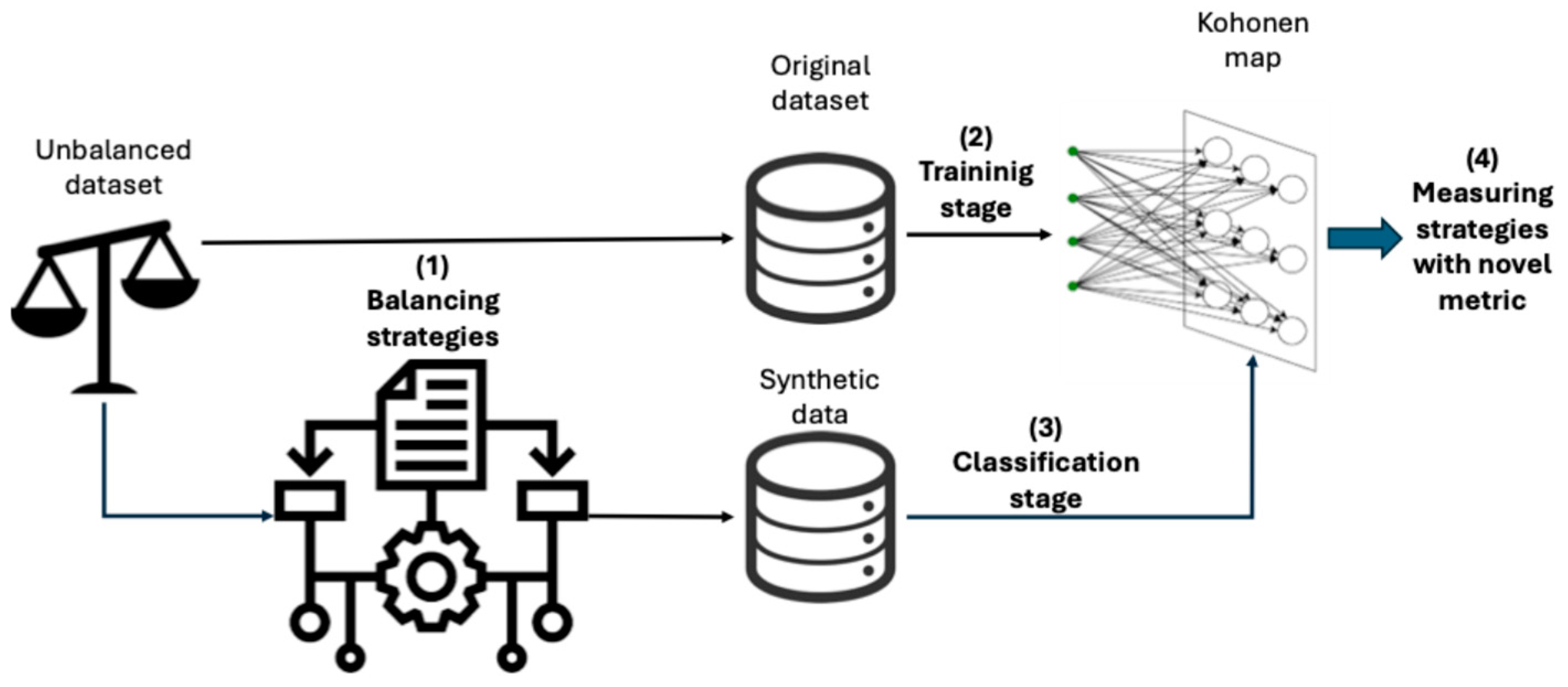
This work is aimed at obtaining a methodology based on SOM so that the best-balancing strategy could be chosen depending on the use case. For this purpose, we have designed the following workflow. First, we choose an unbalanced dataset and apply oversampling and under-sampling strategies for data-balancing. Then, we train a Kohonen map with the original dataset and use SOM to classify the synthetic instances. Even though SOM is not normally used as a classifier, works such as (Winston et al. 2020) benefit from these capabilities. If synthetic data has been well created, it should be classified with low errors (instances that are close in a Euclidean space) in the map trained with original data. As a final way to measure the performance of using the Kohonen map, we use a metric proposed by us. Figure 1 shows how the workflow has been implemented.

Apart from that workflow to choose the performance of the best balancing strategies, we have used Multilayer Perceptrons (MLPs) as a way to confirm that the dataset has been balanced accurately to perform good binary classifications.

3.1. Unbalanced Datasets

The datasets used in this research are described below. In total, we are using 6 datasets: cancer breast, oil spill, German credits, phonemes, microcalcifications and credit card fraud.

First, we find the Haberman dataset for breast classification1. This dataset was compiled by the University of Chicago's Billings Hospital from 1958 to 1970. It comprises a binary classification for patients that died within 5 years or survived 5 years or longer. This classification uses 3 numerical features: age, year of surgery, and the number of positive axillary nodes detected. In total, it has 307 instances.

The second dataset was created from oil spills in satellite radar images2. This dataset was presented by (Kubat, Holte, and Matwin 1998) and compiles satellite images of the ocean, some of them containing oil spills and some not. Images were preprocessed obtaining a set of 49 features that describe the images: area, intensity, or sharpness. The total amount of images is 937.

The third case is called the German credits dataset3. This dataset comprises a set of clients and some financial and banking features to predict if the client will pay back or not a loan or credit. This prediction will be based on 7 integers and 13 categorical variables. These features could be the duration in months, amount, present residence, or job. The information of 1,000 clients was compiled.

Fourth, is the phonemes dataset4. This dataset is aimed to distinguish between nasal and oral sounds. This is performed using a set of 5 features which characterize the amplitude of the first five harmonics normalized by the total energy. In total, an amount of 5,427 examples were compiled.

As a fifth use case, we have a dataset of microcalcifications5. This dataset is used for breast cancer detection from radiological scans. Specifically, it focuses on identifying clusters of microcalcification, which appear bright on mammograms. The dataset was curated by scanning the images, segmenting them into candidate objects, and employing computer vision techniques to characterize each candidate object by using six features.

Finally, the credit card fraud detection dataset6. The dataset comprises transactions conducted by European cardholders using credit cards in September 2013. It only includes numerical input variables resulting from a PCA transformation. 28 features represent the principal components derived from PCA, while the 2 of them remain unaltered by PCA transformation.

Table 1. Dataset summaries.

Dataset	Number of features	Missing values	Classification type		Imbalance
Breast cancer	3	0	Binary numerical	225/81
Oil spills	49	0	Binary numerical	896/41
German credits	20	0	Binary numerical	700/300
Phonemes	5	0	Binary numerical	3,818/1,586
Microcalcifications	6	0	Binary numerical	10,923/260
Credit card fraud	6	0	Binary numerical	284,315/492

Table 1. Dataset summaries.

Dataset	Number of features	Missing values	Classification type		Imbalance
Breast cancer	3	0	Binary numerical	225/81
Oil spills	49	0	Binary numerical	896/41
German credits	20	0	Binary numerical	700/300
Phonemes	5	0	Binary numerical	3,818/1,586
Microcalcifications	6	0	Binary numerical	10,923/260
Credit card fraud	6	0	Binary numerical	284,315/492

3.2. Balancing Strategies

In this paper, we provide an evaluation of strategies to avoid the problem of unbalanced classes in several datasets. There are many types of imbalanced strategies but we have opted for hybrids as they have been shown to create better data distributions and improve the performance in classification problems, (Liu, Liang, and Ni 2011). Hybrid strategies first create synthetic data from the minority class and then, remove instances from both distributions. This not only allows solving the problem of unbalanced classes but also removes noisy instances placed on the wrong side of the cluster frontier. Following, we define all the over and under-sampling strategies that we propose whose combinations will lead to the hybrid strategies we are evaluating in the paper.

Over-sampling strategies. This type of imbalanced strategy creates synthetic instances of the minority class to balance the number of instances per class.

Synthetic Minority Oversampling Technique (SMOTE). Introduced in (Chawla et al. 2002), its main characteristic is that it creates data instances without replacing the original one. SMOTE selects instances of a feature space, drawing a line between them. Then, it uses this line to obtain a point along it which is the new instance.

Adaptive Synthetic Sampling (ADASYN). This method presented by (He et al. 2008) uses a density distribution to automatically determine the number of synthetic samples required for each minority data instance. This density distribution serves as a measure of the weight distribution among various minority class examples, reflecting their respective learning difficulties. Consequently, the dataset after applying the method not only achieves a balanced representation of the data distribution based on the desired balance level but also focuses the learning algorithm's attention on challenging examples.

Borderline SMOTE. As described in (Han, Wang, and Mao 2005), the process involves identifying the borderline examples within the minority class. These borderline instances are then utilized to generate new synthetic examples. These synthesized instances are strategically positioned around the borderline examples of the minority class.

SVM SMOTE. (Nguyen, Cooper, and Kamei 2009) proposed this method that encompasses the following three stages. Firstly, it involves over-sampling the minority class to address data imbalance effectively. Secondly, the sampling strategy is focused primarily on critical regions, particularly the boundary area between classes. Thirdly, it applies extrapolation to extend the minority class region, especially in areas where majority class instances are scarce.

K-Means SMOTE. The approach presented in (Last, Douzas, and Bacao 2017) involves three main steps: clustering, filtering, and over-sampling. Firstly, in the clustering step, the input space is divided into k groups using K-Means. Next, in the filtering step, clusters with a significant proportion of minority class samples are retained for oversampling. Subsequently, the number of synthetic samples to generate is distributed, with more samples assigned to clusters containing sparsely distributed minority samples. Finally, in the over-sampling step, SMOTE is applied within each selected cluster to accomplish the desired ratio between minority and majority instances.

Under-sampling strategies. These strategies involve reducing the number of instances from the majority class to balance the number of instances across classes.

Tomek Links (TL). Regarding (Tomek 1976), this technique removes boundary instances as they have more possibilities to be misclassified. This is based on the definition of the Tomek-link pair which occurs when two instances do not belong to the same class. Then, there is no other sample whose distance to the first instances is lower than the distance between the two individuals. Summarizing, if instances are creating a Tomek-link pair there are more possibilities of having superfluous data along the distribution.

Edited Nearest Neighbor (ENN). Introduced by (Wilson 1972), it aims at refining datasets by removing samples from the majority class that lie close to the decision boundary. If the label of a majority class instance and the labels of applying K-Nearest Neighbors differ, then both the instance and its nearest neighbors are removed from the dataset.

Condensed Nearest Neighbor Rule (CNNR). This is the first selection algorithm as stated in (Hart 1968). It employs two storage areas called Condensing Set (CS) and Training Set (TS) respectively. In the beginning, TS includes the complete training set, while CS remains empty. To initiate the process, an instance is randomly selected from TS and moved to CS. Subsequently, each instance x ∈ TS is compared to those currently stored in CS.

Neighborhood Cleaning Rule (NCL). This algorithm depicted in (Laurikkala 2001) has two stages. The process begins with the application of the Edited Nearest Neighbor algorithm to undersample instances not belonging to the target class. Subsequently, a second step refines the neighbourhood of the remaining examples. Here, the KNN algorithm is applied, removing an example if its neighbours do not belong to the target class and if the example's class exceeds half of the smallest class within the target class.

One Side Selection (OSS). As described in (Kubat, Matwin, and others 1997) the method reduces the number of misclassified instances by creating a subset with the training set. Following this, the method removes misclassified examples involved in Tomek links. This process discards noisy and borderline examples, resulting in the formation of a new training set.

Self-Organizing Maps. SOM which in this work is referred to as Kohonen maps establishes a relation from a higher-dimensional input space to a lower-dimensional map space using a two-layered fully connected architecture. The input layer comprises a linear array with the same number of neurons as the dimension of the input data vector (n). The output layer, known as the Kohonen layer, consists of neurons, each with an associated weight vector of the same dimension as the input data (n) and a position in a rectangular grid of arbitrary size (k). These weight vectors are organized in an n * k * k matrix known as the weight matrix. Self-organization implies that a vector from the input dataset space (X) is presented to the network, and the node with the closest weight vector Wj is identified as the winning neuron or best matching unit (BMU) using a simple discriminant function (Euclidean distance) and a 'winner-takes-all' mechanism (competition). Subsequently, the unsupervised training algorithm adjusts the winner's weight vector based on its similarity to the input vector. This presentation of vectors from the input space and BMU learning continues until a specified number of presentations (P) is reached or values of the selected metrics remain steady. The iterative process yields a trained (self-organized) Kohonen map, represented by a given weight matrix. Each node in the Kohonen layer corresponds to a specific pattern learned during training and can recognize all elements belonging to that class. The self-organizing training process preserves the topological properties of the input space, allowing neighbouring nodes to recognize patterns that are closer in the n-dimensional space, meaning they have similar characteristics. The map generated by this trained SOM can then be used to classify additional input data through a process called "mapping." Unlike training, this process does not alter the weight matrix. New elements from the input space are placed where they are recognized by an existing Best Matching Unit, indicating they are similar (belong to the same class) as those previously recognized by that BMU.

Multilayer perceptron (MLP). This model consists of sequential layers composed of neurons, with each layer connected to adjacent layers. It requires a minimum of three layers: input, hidden, and output. Input data is introduced through the input layer, undergoes processing in the hidden layer, and is classified by the output layer. MLPs optimize parameters through a two-stage backpropagation training process: forward and backward, as described by (Rumelhart, Hinton, and Williams 1986).

4. Results

Following, we describe all the results obtained during the application of our methodology. The results are organized step by step adding some values that helped us during the process and have been used as support material for decision making.

First of all, we need to apply all the strategies to the unbalanced datasets which are 25 combinations in total (5 over-sampling strategies for 5 under-sampling strategies). Then, for each of these combinations, we are training a Kohonen map. For this purpose, we are using a Python library called GEMA developed by (García-Tejedor and Nogales 2022). All the maps have been trained using a grid search strategy which finds the optimal value of the hyperparameters by aggregating various ranges of possibilities, (Bergstra and Bengio 2012). To avoid problems caused by random weights initialization, each neuron in the Kohonen layer takes its weights from one of the input instances. Anyway, based on the main function of SOM which according to (Khalilia and Popescu 2014) is topology preservation of the input data, overall topology tends to remain consistent across instances. In Table 2, we compile all the hyperparameters and values used for this stage.

To find the optimal Kohonen map, we use the quantization and the topographic error. The quantization error represents the mean distance between each data vector and its BMU. Calculated for the winning neurons, this metric is independent of the number of "empty" neurons and the size of the map, serving as a measure of map resolution. This error is defined in Equation 1.

$$QE={\displaystyle \frac{1}{N}}{\sum }_{i=1}^N‖X_i-{BMU}_{\left(i\right)}‖$$

(1)

As is denoted above $N$ is the number of instances in the training datasets and $X_i$ an input vector.

Meanwhile, the topographic error indicates the ratio of all data vectors for which the first and second BMUs are not adjacent units, providing insight into topology preservation. Equation 2 defines the topographic error.

$$TE={\displaystyle \frac{1}{N}}{\sum }_{i=1}^N{t(x}_i)$$

(2)

where ${t(x}_i)$ equals 0 if the BMU and the second-best matching units are adjacent, otherwise its value is 1; and $N$ is the total number of instances.

In the following Table 3, Table 4, Table 5, Table 6, Table 7 and Table 8, we show for each selected dataset both metrics for all the combinations of imbalanced strategies applied to each dataset using GEMA.

In the tables above, the top 5 strategies have been bolded. These strategies are considered the best as they combine lower values for both quantization and topological errors. Besides, the best one has been highlighted. As we can see, the best strategies change depending on the library but in some datasets, a few of the top strategies are the same and even the best one matches.

In Table 3, SMOTE combined with ENN, CNN and NCR and ADASYN with CNN and NCR are in the top 5 for both strategies. In Table 4, we found again ADASYN plus CNN and TL. The combination of Borderline SMOTE plus TL, and CNN are the other highlighted strategies. Regarding Table 5, we have SMOTE with ENN and OSS, ADASYN with CNN and OSS and K-Means SMOTE with OSS. In Table 6, we can find the following strategies in both tops: ADAYSN combined with TL, ENN or NCR and K-Means SMOTE with OSS. Then, we have Table 7 where K-Means SMOTE with ENN is at the top and the best. Then, K-Means SMOTE with CNN, NCR and OSS and ADASYN with NCR are also on the top. Finally, we have Table 8 with SVM SMOTE combined with the five other strategies. As can be seen, the best strategies are very distributed with only two of them being three times on the top: ADASYN plus NCR and K-Means SMOTE with OSS.

As the differences in the error metrics between different strategies are very low in most of the cases, we can conclude that errors are intuitive but not conclusive. Based on that, we proposed a new metric using the topology provided by the Kohonen maps. The idea is that neurons of the map trained with the unbalanced dataset should recognize similar input vectors when mapping the balanced dataset. So, topological changes from one map to another should be small. For this, we use the instance of the map that we consider the best trained which are those with the lowest errors.

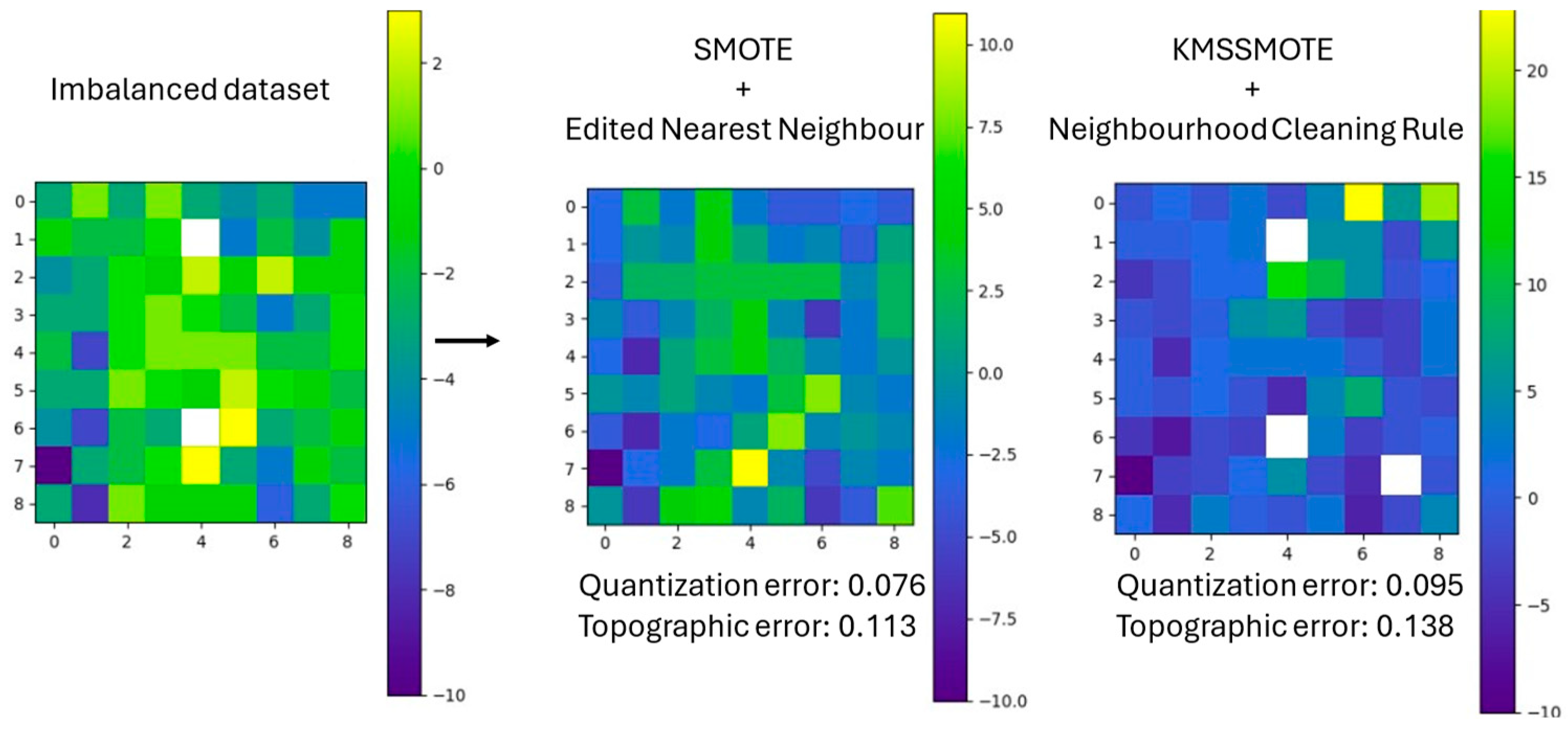
To validate this assumption, we use two derived graphical representations of the Kohonen maps. The first uses a heatmap that indicates differences between the number of synthetic instances recognized by the neurons that belong to each class. If neurons recognize more instances of the minority class, they are yellow-coloured changing to blue when the neurons recognize more instances of the majority class. Empty neurons are left blank.

The second map uses four colours depending on how neurons perform recognizing instances of the two classes in the datasets. Empty neurons are left blank, indicating they recognize no instances at all. Red and blue neurons recognize a percentage of instances from both the original and synthetic data, corresponding to the minority and majority classes, respectively. This value acts as a threshold that can be varied to perform different analyses, where the percentage of instances from one of the two classes must exceed this threshold to colour the neuron with the corresponding class colour. Finally, green neurons represent a balance, recognizing instances from both classes.

In Figure 2, we show an example for the first type of map and in Figure 3 the same for the map with pure colours. In both Figures, we show the map with the imbalanced dataset, then a map obtained after using the strategies with the lowest error (those that allegedly created the best synthetic data) and then, the map with the highest one (those that allegedly created the worst synthetic data).

These maps support the notion that the strategies that yield lower errors are those that generate synthetic data closely resembling the original class instances. This indicates that successful strategies create synthetic samples that maintain the characteristics and distribution of the original data, thereby improving model performance. As can be seen, in both Figures changes from the first map to the second one are lower which indicates that the created instances by the balancing strategies are closer to the original dataset. For example, if a red or blue neuron (indicating recognition of many instances of one class) changes to the opposite colour, we can infer that the synthetic data is of poor quality. This is because the model is confusing the synthetic data to such an extent that a neuron, which should primarily detect one class, is now detecting many instances of the opposite class. Conversely, if a green neuron, which is on the borderline of being pure, turns red or blue, there is no immediate issue. This simply means it has recognized one additional instance of one of the classes, making it a pure neuron. Similarly, if a red or blue neuron becomes green, it indicates that it has recognized one more instance of the opposite class, making it non-pure, which is also not problematic. At this point, we have demonstrated that for a given use case, when a SOM trained with the unbalanced dataset classifies data generated by the best balancing strategies (those that produce maps with the lowest quantization and topological errors), the mapping process exhibits only slight changes. This indicates that the best balancing strategies create synthetic data that closely matches the original data distribution, maintaining the integrity and effectiveness of the SOM's classification capabilities.

However, these metrics have minimum differences, so we need to obtain a way to measure the validity of the different balancing strategies. For this purpose, we proposed our metric based on the idea described above. The similarity is based on the Jaccard index introduced in (Jaccard 1912) and defined in the following Equation.

$$J(A,B)={\displaystyle \frac{\left|A\cap B\right|}{\left|A\cup B\right|}}={\displaystyle \frac{\left|A\cap B\right|}{\left|A\right|+\left|B\right|-\left|A\cap B\right|}}$$

(3)

Where A and B are two different sets, ∣A∩B∣ is the number of elements in the intersection of sets A and B and ∣A∪B∣ is the number of elements in the union of both sets. The Jaccard index ranges from 0 to 1, where 0 indicates that the two sets are disjoint (no common elements) and 1 indicates that the two sets are identical.

We have adapted this index to the graphical representation of the Kohonen maps which we have named the Similarity Over Maps (SOM) Jaccard index. The two sets correspond to the mapping of the original dataset and the mapping after applying balancing strategies respectively. Our index results of applying the Jaccard index to red, blue and green-coloured neurons. Then, we average the value giving a percentage of similarity. This metric is formalized as follows.

$${SOM}_{Jaccard}({KM}_1,{KM}_2)={\displaystyle \frac{{J({KM}_1,{KM}_2)}_{RED}+{J({KM}_1,{KM}_2)}_{BLUE}+{J({KM}_1,{KM}_2)}_{GREEN}}{3}}$$

(4)

Following, we present the values of our metric after applying the balancing strategies to the six proposed datasets. All this information is compiled in Table 9, Table 10, Table 11, Table 12, Table 13 and Table 14, one for each dataset.,. The columns of the Tables show different percentages that correspond to the threshold that considers a neuron as pure (red or blue). We only show the top 3 strategies performing better with our metric

As can be seen, the threshold seems to have minimal impact, except for the 65% case, which shows big differences. So, we have selected a threshold of 80% as it allows us to identify pure neurons more accurately. If we look at the strategies separately, we can conclude that the differences also are not very high, and they remain stable. The one marked as the best does not stand out too much from the others but let us consider it as the best.

Now, as half of the datasets are unbalanced at around 40% and half are around 90%, we want to compare the performance of the strategies between datasets. Table 15 compiles the information related to the average and standard deviation of applying all the strategies. The results above show that the percentage of unbalanced data does not affect the quality of the synthetic dataset.

To establish an additional criterion for evaluating the effectiveness of the strategies, we have analysed the frequency with which each strategy appears in the top three rankings across Table 9. This approach allows us to identify which strategies consistently perform well and are therefore more reliable in achieving optimal results. In the following Table, we can see this top.

As can be seen, only SMOTE+ENN stands out against the rest of the strategy. This fits in with the results obtained with the Kohonen maps errors where this strategy was considered many times as one of the best.

Finally, we have trained an MLP using a grid search strategy for each of the datasets that have better metrics in the previous Tables. Based on these results we just pretend to demonstrate that metrics with synthetic datasets perform accurately and do not overfit. In the following Table, we show the accuracy metrics in training, validation, and testing for the best-balancing strategies in each dataset. Results show average values and standard deviation after applying k-fold validation.

Table 17. Trained MLPs after applying the best-balancing strategy for each dataset.

Dataset	Training	Validation	Test
Bank loans	90.4% ± 1.8%	86.2% ± 2.5%	82.7%
Phonemes	81.3% ± 5%	80.6% ± 4.5%	78%
Breast cancer	97.3% ± 0.8%	89.0% ± 6.0%	87.3%
Credit frauds	99.7% ± 0.2%	99.6% ± 0.3%	99.8%
Oil spills	93.9% ± 0.8%	93.6% ± 0.7%	93.4%
Microcalcifications	93.9% ± 0.8%	93.6% ± 0.7%	93.4%

Table 17. Trained MLPs after applying the best-balancing strategy for each dataset.

Dataset	Training	Validation	Test
Bank loans	90.4% ± 1.8%	86.2% ± 2.5%	82.7%
Phonemes	81.3% ± 5%	80.6% ± 4.5%	78%
Breast cancer	97.3% ± 0.8%	89.0% ± 6.0%	87.3%
Credit frauds	99.7% ± 0.2%	99.6% ± 0.3%	99.8%
Oil spills	93.9% ± 0.8%	93.6% ± 0.7%	93.4%
Microcalcifications	93.9% ± 0.8%	93.6% ± 0.7%	93.4%

As can be seen, for all the datasets the MLPs obtain good results as they accomplish the bias-variance trade-off, (Belkin et al. 2019). In terms of bias, the values of the metrics are good enough. If we look at the variance, differences between train, validation and test are low. If we look at the standard deviations, we can conclude that all the models are very stable. The experiments in this table, let us know that synthetic data is good enough as MLPs are obtaining good metrics.

5. Conclusions and Future Works

This paper proposes a methodology using Kohonen maps to evaluate various imbalanced data strategies. We applied a combination of five over-sampling and undersampling techniques to create synthetic data, resulting in a total of 25 different methods. Initially, we assessed the performance of these strategies using two SOM metrics: topological and quantization errors. These metrics, derived from training and applying the strategies to six different datasets, indicated which strategies performed better. Given the minimal differences between these errors, we introduced a new metric based on the topological properties of Kohonen maps, applied to the best results obtained so far. This metric was applied to all strategies across the six datasets, and its potential was demonstrated by training six MLPs (one for each dataset) using the best-performing imbalanced strategies according to our metric.

The main limitation of this study is the variation in the number of imbalanced instances between classes within the datasets. Additionally, the datasets differ in total instances and the number of features per individual.

In future work, we aim to apply this methodology to real-world cases where data imbalance is due to scarcity. By generating synthetic data to balance these datasets, we hope to improve the performance of classifiers that previously struggled with imbalanced data.

References

- Belkin, Mikhail, Daniel Hsu, Siyuan Ma, and Soumik Mandal. 2019. “Reconciling Modern Machine-Learning Practice and the Classical Bias--Variance Trade-Off.” Proceedings of the National Academy of Sciences 116(32): 15849–54. [CrossRef]
- Bergstra, James, and Yoshua Bengio. 2012. “Random Search for Hyper-Parameter Optimization.” Journal of machine learning research 13(2).
- Chawla, Nitesh V, Kevin W Bowyer, Lawrence O Hall, and W Philip Kegelmeyer. 2002. “SMOTE: Synthetic Minority over-Sampling Technique.” Journal of artificial intelligence research 16: 321–57.
- Chawla, Nitesh V, Aleksandar Lazarevic, Lawrence O Hall, and Kevin W Bowyer. 2003. “SMOTEBoost: Improving Prediction of the Minority Class in Boosting.” In Knowledge Discovery in Databases: PKDD 2003: 7th European Conference on Principles and Practice of Knowledge Discovery in Databases, Cavtat-Dubrovnik, Croatia, September 22-26, 2003. Proceedings 7, , 107–19.
- Choirunnisa, Shabrina, and Joko Lianto. 2018. “Hybrid Method of Undersampling and Oversampling for Handling Imbalanced Data.” In 2018 International Seminar on Research of Information Technology and Intelligent Systems (ISRITI), , 276–80.
- Costa, Afonso José, Miriam Seoane Santos, Carlos Soares, and Pedro Henriques Abreu. 2020. “Analysis of Imbalance Strategies Recommendation Using a Meta-Learning Approach.” In 7th ICML Workshop on Automated Machine Learning (AutoML-ICML2020), , 1–10.
- Dong, Qi, Shaogang Gong, and Xiatian Zhu. 2018. “Imbalanced Deep Learning by Minority Class Incremental Rectification.” IEEE transactions on pattern analysis and machine intelligence 41(6): 1367–81.
- García-Tejedor, Álvaro José, and Alberto Nogales. 2022. “An Open-Source Python Library for Self-Organizing-Maps.” Software Impacts 12. [CrossRef]
- Goel, Garima, Liam Maguire, Yuhua Li, and Sean McLoone. 2013. “Evaluation of Sampling Methods for Learning from Imbalanced Data.” In International Conference on Intelligent Computing, , 392–401.
- Gosain, Anjana, and Saanchi Sardana. 2017. “Handling Class Imbalance Problem Using Oversampling Techniques: A Review.” In 2017 International Conference on Advances in Computing, Communications and Informatics (ICACCI), , 79–85.
- Han, Hui, Wen-Yuan Wang, and Bing-Huan Mao. 2005. “Borderline-SMOTE: A New over-Sampling Method in Imbalanced Data Sets Learning.” In International Conference on Intelligent Computing, , 878–87.
- Hart, Peter. 1968. “The Condensed Nearest Neighbor Rule (Corresp.).” IEEE transactions on information theory 14(3): 515–16.
- He, Haibo, Yang Bai, Edwardo A Garcia, and Shutao Li. 2008. “ADASYN: Adaptive Synthetic Sampling Approach for Imbalanced Learning.” In 2008 IEEE International Joint Conference on Neural Networks (IEEE World Congress on Computational Intelligence), , 1322–28.
- Jaccard, Paul. 1912. “The Distribution of the Flora in the Alpine Zone. 1.” New phytologist 11(2): 37–50.
- Johnson, Justin M, and Taghi M Khoshgoftaar. 2019. “Survey on Deep Learning with Class Imbalance.” Journal of Big Data 6(1): 1–54. [CrossRef]
- Junsomboon, Nutthaporn, and Tanasanee Phienthrakul. 2017. “Combining Over-Sampling and under-Sampling Techniques for Imbalance Dataset.” In Proceedings of the 9th International Conference on Machine Learning and Computing, , 243–47.
- Khalilia, Mohammed, and Mihail Popescu. 2014. “Topology Preservation in Fuzzy Self-Organizing Maps.”. [CrossRef]
- Kohonen, Teuvo. 1982. “Self-Organized Formation of Topologically Correct Feature Maps.” Biological Cybernetics 43(1): 59–69. [CrossRef]
- Kohonen, Teuvo. 1998. “The Self-Organizing Map.” Neurocomputing 21(1): 1–6. [CrossRef]
- Kraiem, Mohamed S., Fernando Sánchez-Hernández, and María N. Moreno-García. 2021. “Selecting the Suitable Resampling Strategy for Imbalanced Data Classification Regarding Dataset Properties. An Approach Based on Association Models.” Applied Sciences (Switzerland) 11(18). [CrossRef]
- Kubat, Miroslav, Robert C Holte, and Stan Matwin. 1998. “Machine Learning for the Detection of Oil Spills in Satellite Radar Images.” Machine learning 30(2): 195–215. [CrossRef]
- Kubat, Miroslav, Stan Matwin, and others. 1997. “Addressing the Curse of Imbalanced Training Sets: One-Sided Selection.” In Icml, , 179.
- Last, Felix, Georgios Douzas, and Fernando Bacao. 2017. “Oversampling for Imbalanced Learning Based on K-Means and Smote.” arXiv preprint arXiv:1711.00837.
- Laurikkala, Jorma. 2001. “Improving Identification of Difficult Small Classes by Balancing Class Distribution.” In Conference on Artificial Intelligence in Medicine in Europe, , 63–66.
- Liu, Tong, Yongquan Liang, and Weijian Ni. 2011. “A Hybrid Strategy for Imbalanced Classification.” In 2011 3rd Symposium on Web Society, , 105–10.
- Mujahid, Muhammad, E. R.O.L. Kına, Furqan Rustam, Monica Gracia Villar, Eduardo Silva Alvarado, Isabel De La Torre Diez, and Imran Ashraf. 2024. “Data Oversampling and Imbalanced Datasets: An Investigation of Performance for Machine Learning and Feature Engineering.” Journal of Big Data 11(1). [CrossRef]
- Nguyen, Hien M, Eric W Cooper, and Katsuari Kamei. 2009. “Borderline Over-Sampling for Imbalanced Data Classification.” In Proceedings: Fifth International Workshop on Computational Intelligence \& Applications, , 24–29.
- Pérez, Joaqu\’\in, Emmanuel Iturbide, V\’\ictor Olivares, Miguel Hidalgo, Nelva Almanza, and Alicia Mart\’\inez. 2015. “A Data Preparation Methodology in Data Mining Applied to Mortality Population Databases.” In New Contributions in Information Systems and Technologies, Springer, 1173–82. [CrossRef]
- Raeder, Troy, George Forman, and Nitesh V Chawla. 2012. “Learning from Imbalanced Data: Evaluation Matters.” In Data Mining: Foundations and Intelligent Paradigms, Springer, 315–31.
- Rumelhart, David E, Geoffrey E Hinton, and Ronald J Williams. 1986. “Learning Representations by Back-Propagating Errors.” nature 323(6088): 533–36.
- Santoso, B, H Wijayanto, K A Notodiputro, and B Sartono. 2017. “Synthetic over Sampling Methods for Handling Class Imbalanced Problems: A Review.” In IOP Conference Series: Earth and Environmental Science, , 12031. [CrossRef]
- Shamsudin, Haziqah, Umi Kalsom Yusof, Andal Jayalakshmi, and Mohd Nor Akmal Khalid. 2020. “Combining Oversampling and Undersampling Techniques for Imbalanced Classification: A Comparative Study Using Credit Card Fraudulent Transaction Dataset.” In 2020 IEEE 16th International Conference on Control \& Automation (ICCA), , 803–8.
- Sun, Aixin, Ee-Peng Lim, and Ying Liu. 2009. “On Strategies for Imbalanced Text Classification Using SVM: A Comparative Study.” Decision Support Systems 48(1): 191–201. [CrossRef]
- Tomek, Ivan. 1976. “AN EXPERIMENT WITH THE EDITED NEAREST-NIEGHBOR RULE.”.
- Wainer, Jacques, and Rodrigo A Franceschinell. 2018. “An Empirical Evaluation of Imbalanced Data Strategies from a Practitioner’s Point of View.” arXiv preprint arXiv:1810.07168.
- Wilson, Dennis L. 1972. “Asymptotic Properties of Nearest Neighbor Rules Using Edited Data.” IEEE Transactions on Systems, Man, and Cybernetics (3): 408–21. [CrossRef]
- Winston, J. Jenkin, Gul Fatma Turker, Utku Kose, and D. Jude Hemanth. 2020. “Novel Optimization Based Hybrid Self-Organizing Map Classifiers for Iris Image Recognition.” International Journal of Computational Intelligence Systems 13(1): 1048–58. [CrossRef]
- Wongvorachan, Tarid, Surina He, and Okan Bulut. 2023. “A Comparison of Undersampling, Oversampling, and SMOTE Methods for Dealing with Imbalanced Classification in Educational Data Mining.” Information (Switzerland) 14(1). [CrossRef]