1. Introduction
Over the past few decades, due to changes in forest ecosystems resulting from both natural and anthropogenic activities, there has been an increased demand for precise and accurate spatial information about forest ecosystems [
1,
2,
3,
4]. Making informed decisions in forest management is based on high-quality data collected during forest inventories [
5], which are most commonly conducted in the field, making the process exceptionally time-consuming and costly [
6,
7]. In addition to conventional terrestrial methods of data collection, forest data (such as tree location, height, diameter at breast height, volume, etc.) are increasingly being gathered using remote sensing methods. The application of remote sensing methods improves forest inventories [
8], reduces the scope of fieldwork, and provides opportunities for time and cost savings [
2,
9,
10,
11]. Data obtained through remote sensing methods have advantages over field-collected data, as they allow for the prediction of forest characteristics and are not spatially restricted to areas covered by forest inventory programs [
12]. For an entire century, photogrammetry has been used as an efficient and high-quality method of measurement without direct contact with the object. However, with the continuous development and advancement of technology, the scope and potential applications of remote sensing methods and techniques are expanding [
13]. Over the past two decades, spatial laser scanning technology, specifically LiDAR [
14], has emerged as a fully automated and highly efficient data collection method. This technology has undergone rapid development, evolving from scientific investigations to operational applications [
15]. With the emergence of LiDAR as an active remote sensing technology, it is now possible to obtain information and parameters related to the vertical structure of features, particularly trees [
7], offering a cost-effective alternative to traditional field-based and two-dimensional remote sensing methods [
6,
16]. The rapid adoption of Light Detection and Ranging (LiDAR) technologies on various platforms (satellites, aircraft, unmanned aerial vehicles) enables the acquisition of fast and precise three-dimensional information about the structural properties of forests and the assessment of their changes [
17,
18,
19,
20,
21,
22,
23,
24,
25,
26,
27,
28,
29,
30]. The most popular technology for studying forest structure is airborne laser scanning (ALS), while terrestrial laser scanners (TLS) and handheld mobile laser scanners are also used to some extent [
31,
32]. The popularity of ALS is not only due to its ability to provide accurate height estimates over large areas [
33], but also because the laser signal can penetrate gaps in vegetation, allowing for measurements of the ground and the internal structure of trees [
6], as well as for measuring height growth [
34,
35,
36,
37]. ALS enables a more detailed assessment of these properties in both space and time, facilitating the practical application of more complex forest management systems [
38,
39]. According to Slavik et al. [
40], a special case of the aforementioned method is data collection using unmanned aerial vehicles (UAVs) equipped with a LiDAR sensor—UAV laser scanning (ULS). In recent years, UAV laser scanning has gained attention due to its safety, data collection flexibility, and high-quality data compared to ALS, all attributed to the UAV's ability to fly at lower speeds and altitudes above the ground. Point clouds derived from unmanned aerial vehicle (UAV) imagery are widely recognized in forestry due to their cost-effectiveness and ability to provide information on canopy structures over larger areas [
41,
42,
43,
44,
45]. LiDAR systems have become one of the key methods for obtaining data on the structure, changes, and spatial distribution of forest resources, owing to their fast and accurate results [
46]. They offer significant advantages for operational forest inventories [
30] and are increasingly being applied in the monitoring of structural parameters [
2].
The total area of forests and forest land in the Republic of Croatia amounts to 2,759,039 ha, which constitutes 49.3% of the country's land area. The fundamental principles of Croatian forestry are sustainable management while preserving the natural structure and biodiversity of forests, as well as the continuous improvement of the stability and quality of both economic and public-benefit functions of forests. The application of modern data collection methods (LiDAR), along with the use of GIS technology, which enables the integration of various types of collected data into a cohesive whole, significantly increases the speed of data preparation for planning and implementing forest management activities.
The main objectives of this study was to measure the structural elements of the stand (volume, basal area, tree count, height, diameter at breast height, crown width and area, etc.) using LiDAR imagery, assess the accuracy of the obtained results and to investigate the possibilities of rationalizing the implementation of forest inventories based on the developed models.
Within the systematic sampling grid (100x100 m), commonly used in field measure-ments, and considering the variability, area, and age of the stand, the smallest acceptable sample plot will be tested through random selection. This will ensure the achievement of equal measurement accuracy, ultimately contributing to a reduction in the time and costs of forest inventory planning.
2. Materials and Methods
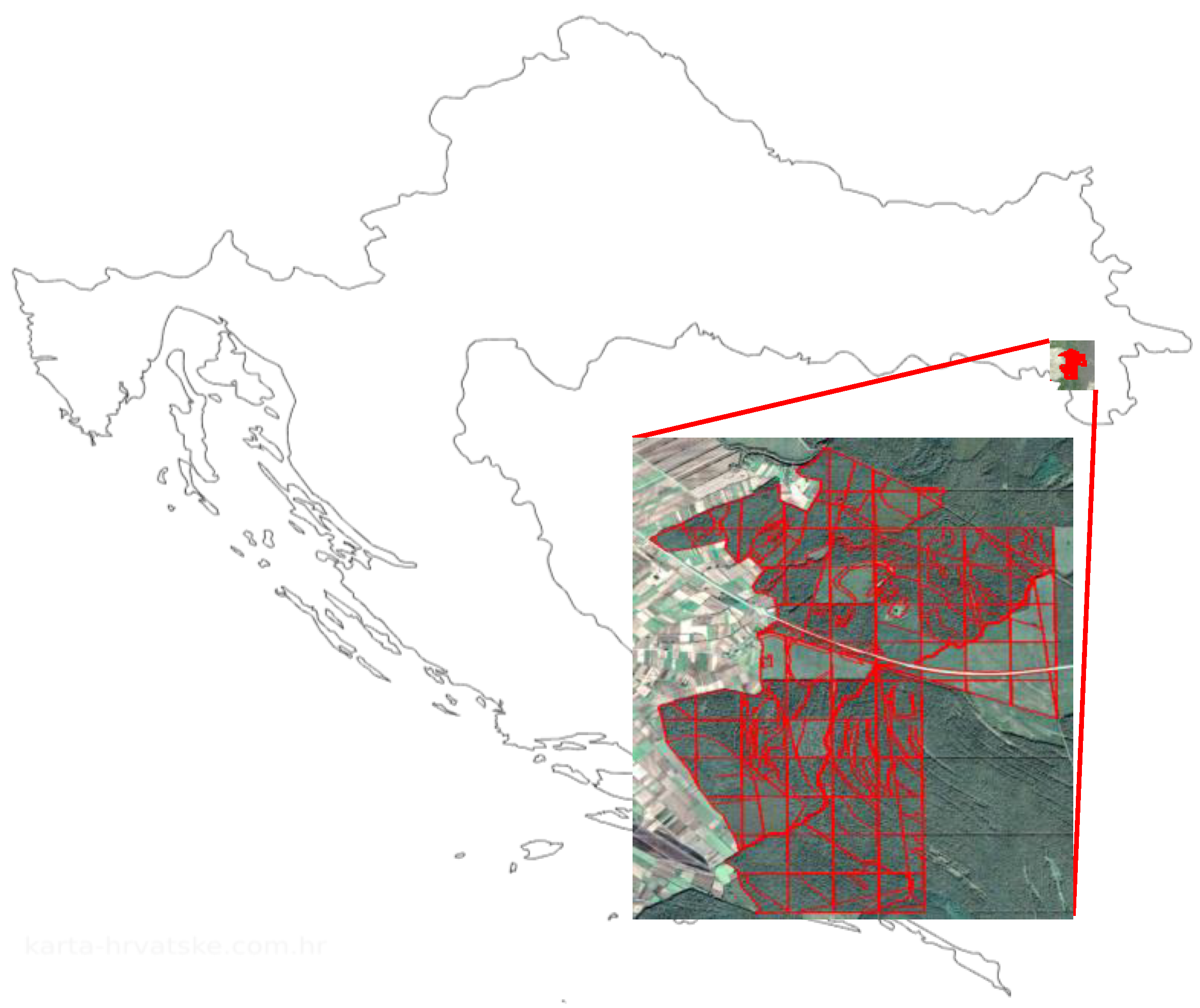
The study was conducted in the most valuable forests in the Republic of Croatia – the lowland pedunculate oak forests, covering an area of 5500 ha. For the area included in the study (
Figure 1), a selection of representative stands for scanning was made. This was followed by a field survey and inspection of the selected stands.
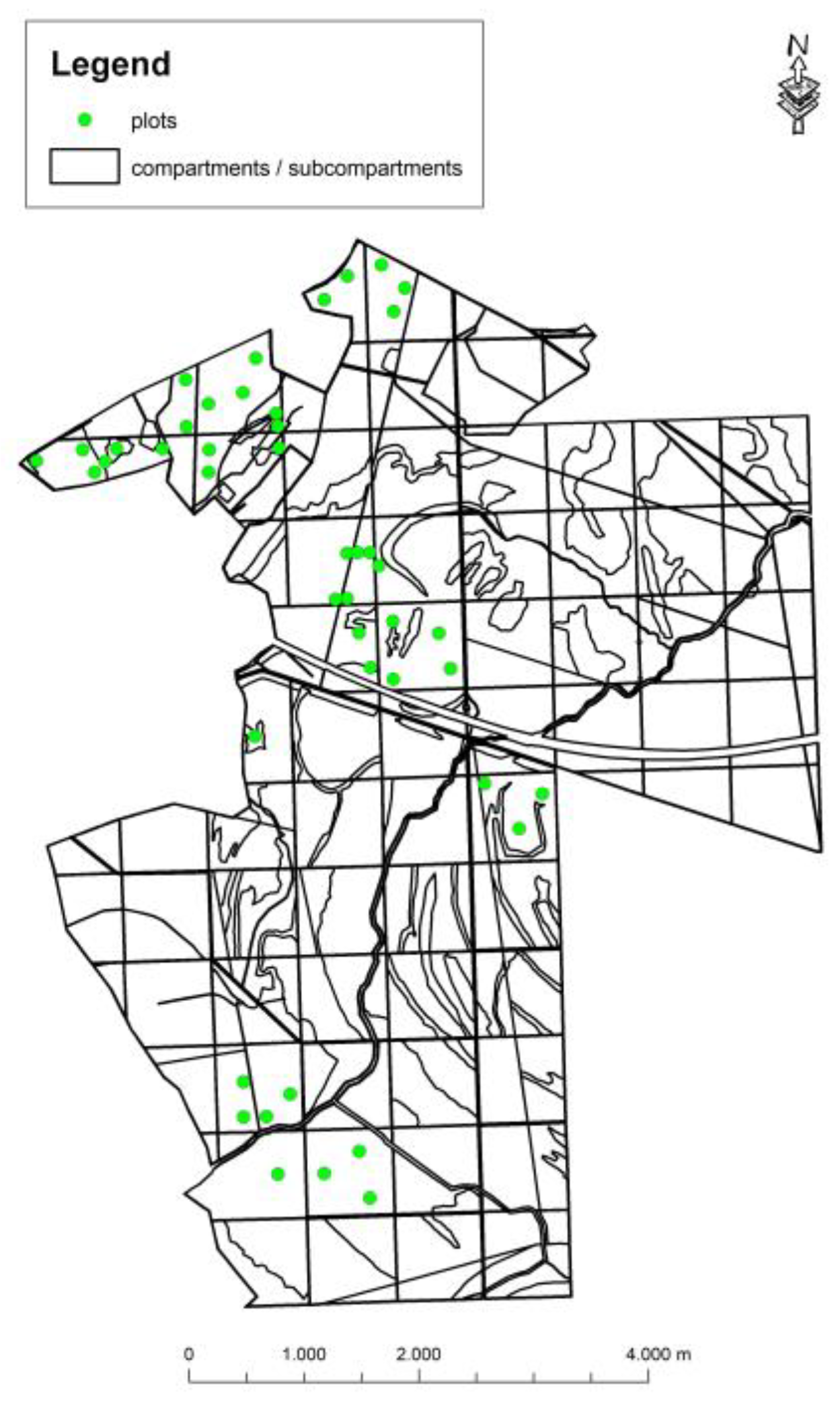
Since the study was aligned with regular forest management on the defined area, and the measurement of structural parameters was carried out on a systematic 100 x 100 m grid, a random sample of field plots (radius 13 m) was designed within the existing systematic sample. This was done for direct measurements and assessments of tree and stand variables in the field, and later on the imagery. The plots were selected based on the principle of representing an appropriate number of stands, or plots, within each age class (I. 1-20 years, II. 20-40 years, III. 40-60 years, IV. 60-80 years, V. 80-100 years, VI. 100-120 years, VII. 120-140 years) and forest type (
Figure 2).
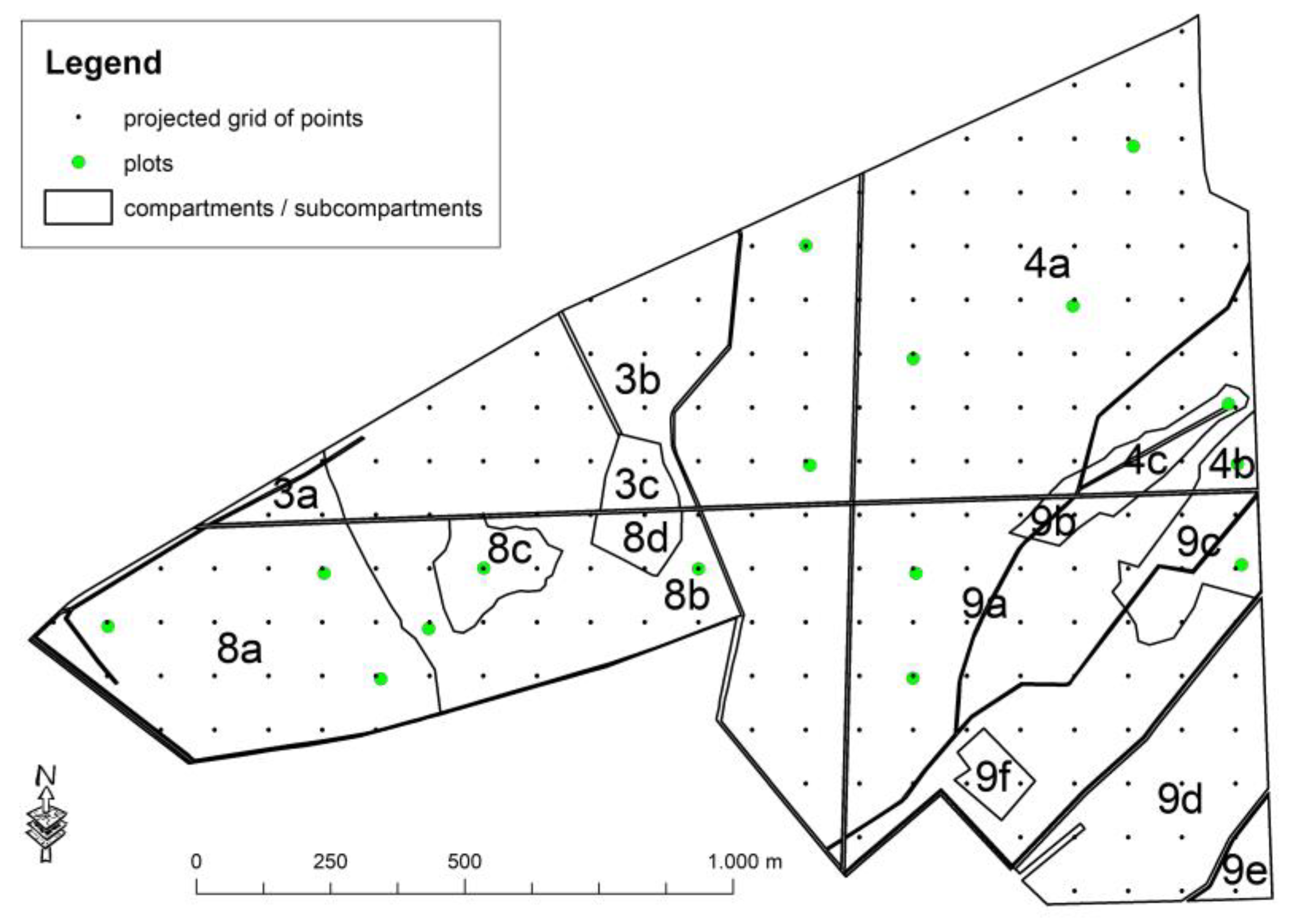
The centers of the selected plots (radius 13 m) were then defined on the designed systematic sampling grid, i.e., the coordinates of the plot centers were determined to ensure that the plots could be matched in the field during the interpretation (measurement) of the imagery. Overview maps of the study area with the designed plot sample were created (
Figure 3).
The coordinates of the plot centers in the field, within the systematic sampling grid, were precisely determined using an RTK GNSS Trimble device to ensure that the plot center in the field exactly matched the plot center during the interpretation of the imagery. This allowed for the comparison of parameters for the same trees measured using different methods. In addition to the variables typically measured during regular forest management, the tree measurements also included time consumption and the determination of the spatial position of the sampled trees.
Regarding the measurement process, on each plot designated for measurement (random selection), all trees were marked and numbered with color, tree species were identified, and for each tree, two perpendicular diameters were measured using a caliper (accuracy of 1 cm). Tree heights were measured using a Vertex instrument. Distances and angles (azimuth) were also measured for each tree relative to the plot center, thereby obtaining the spatial distribution of the measured trees. For each plot, the time required to measure all the aforementioned parameters (start and end of the measurement) was recorded.
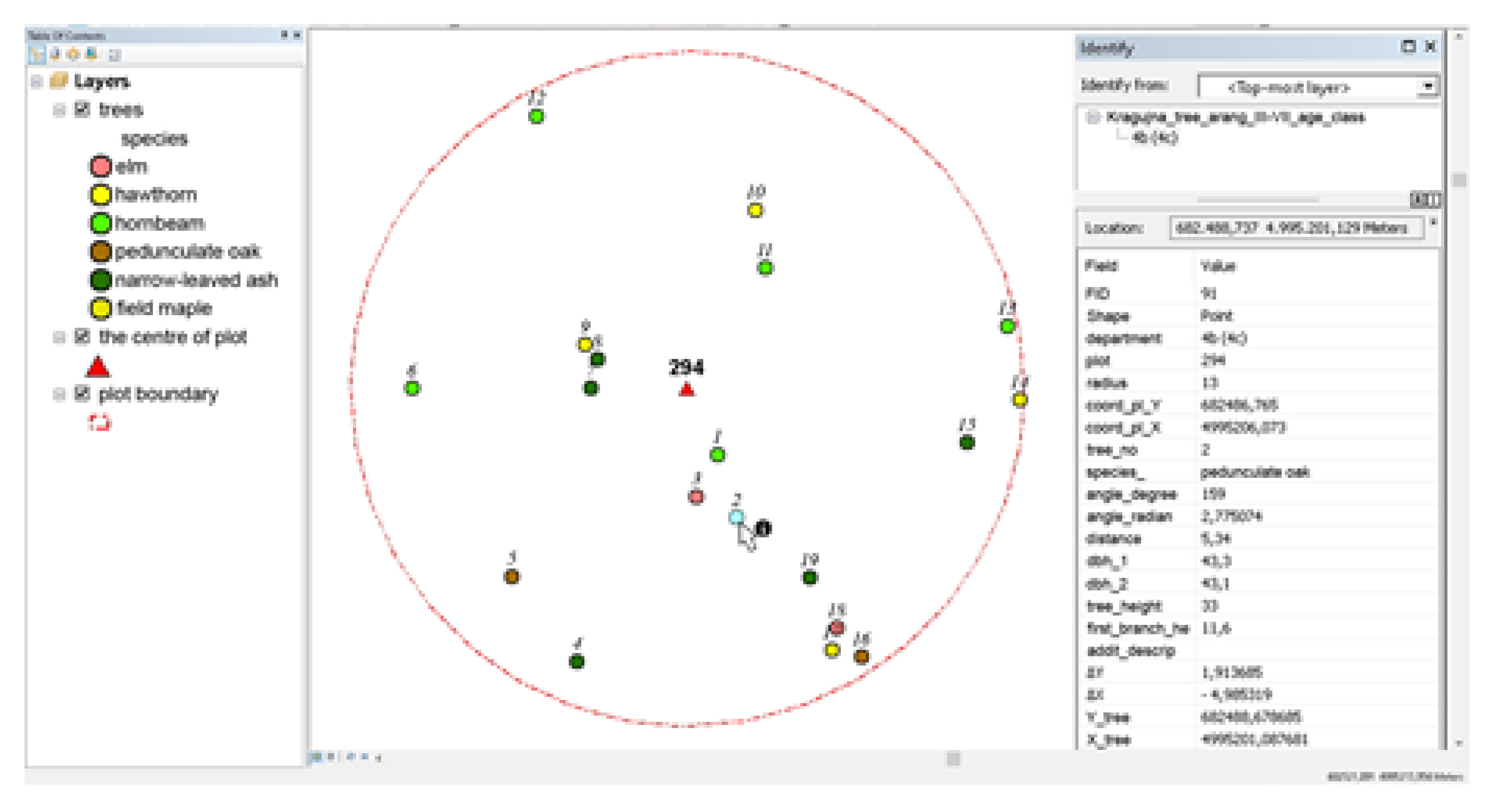
After the field measurements were conducted, a database was created for each management unit in GIS (ArcGIS 10.x), containing all measured parameters: compartment/subcompartment, plot number, X-Y coordinates, tree number, species, distance and angle relative to the plot center, two perpendicular breast heights, tree height, height to the first branch, and the start and end times of the measurement on the plot (
Figure 4).
Based on the data obtained from the field measurements, the volume, basal area, tree count, mean stand height, and mean stand diameter were calculated.
The research area was recorded by an unmanned aerial vehicle (DJI Matrice 300 RTK), with 3 flights at a height of 80 m. After the aerial photogrammetry (RGB - DJI Zenmuse P1) and laser (LiDAR - DJI Zenmuse L1 lidar) data were conducted, the images were prepared and processed for measurement.
Regarding LiDAR, the "raw" point cloud – 473 points/m2 (*.las format) needed to be classified and filtered, followed by the normalization of point heights, and then the classification and segmentation of vegetation into individual trees, shrubs, etc (software GreenValley LiDAR360).
The orthorectified images were loaded with a systematic sampling grid of 100x100 m (plot centers) and randomly selected plots of appropriate dimensions, i.e., the same plots where the field measurements were conducted. Each loaded plot was clipped from the image and underwent point cloud processing procedures in several phases:
"Cleaning" of the point cloud, i.e., mitigation of "noise"
Classification of points representing the ground (separation of ground points from vegetation)
Normalization of the point cloud (conversion of elevation values to heights above ground level)
Automatic segmentation of vegetation (individual trees, shrubs, and other vegetation types)
Manual correction of segmented trees (if necessary)
Measurement of segmented trees (tree coordinates, diameter at breast height, height, crown width, etc.), i.e., determination of parameters as in operational forest management.
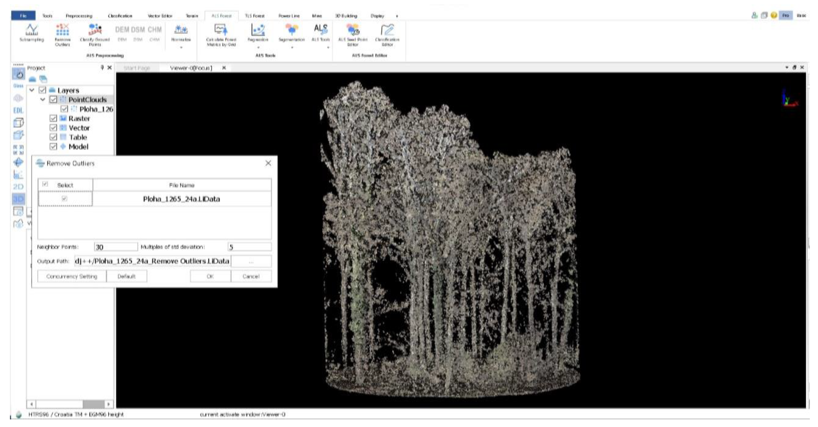
The first phase of LiDAR data processing involves point cloud cleaning (e.g., some points in the cloud significantly deviate from others and, as such, do not represent trees, but instead create errors in subsequent processing). Point cloud cleaning is performed automatically (
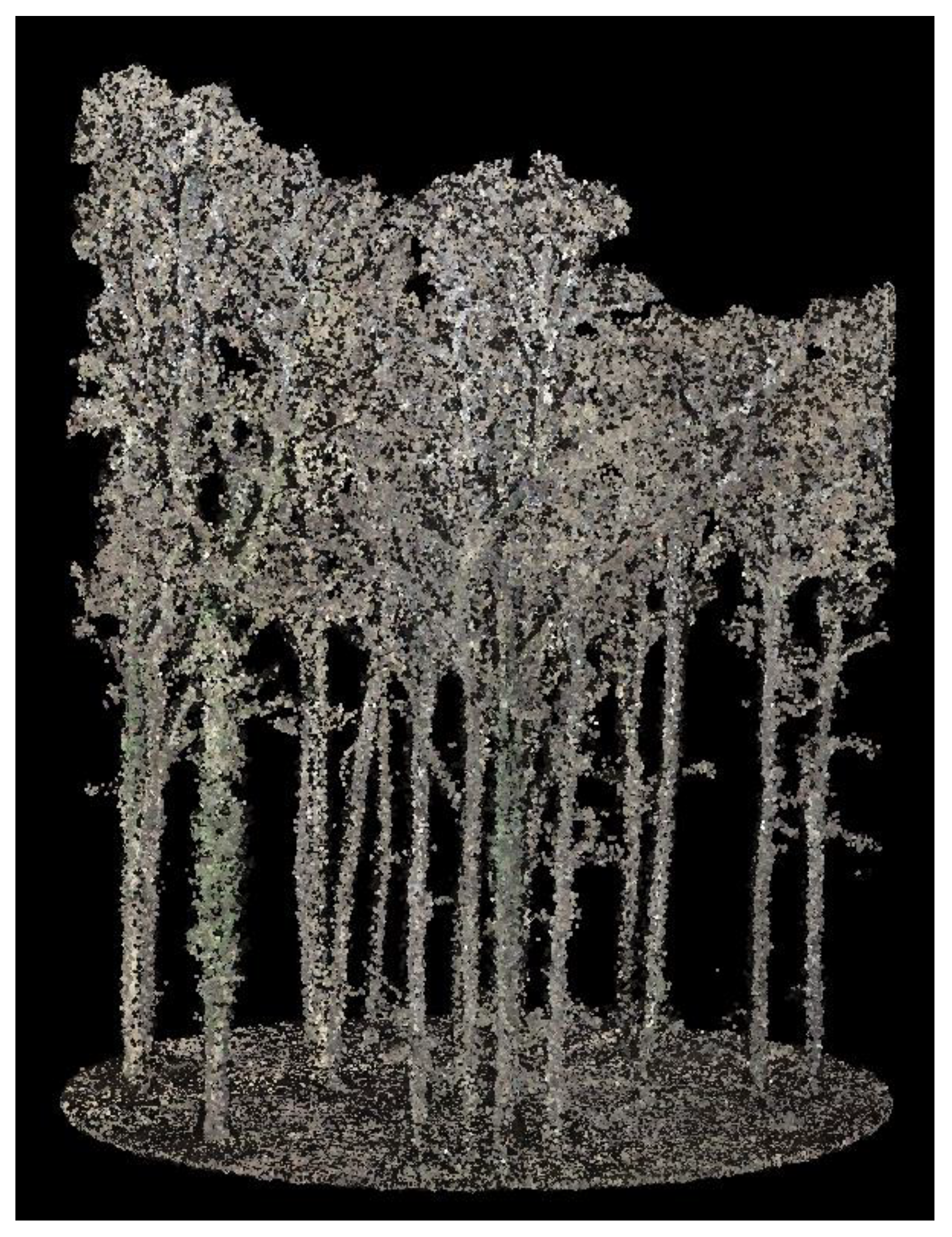
Figure 5) and/or manually, until all points that could impact the measurement are removed. This results in a higher-quality point cloud, with reduced presence of "noise", while simultaneously increasing the accuracy of automatic measurements (
Figure 6).
After this processing, the image was ready for further procedures, which included ground classification and, based on the ground classification, point height normalization. This process converted the elevation values of the vegetation points into values representing heights above the ground.
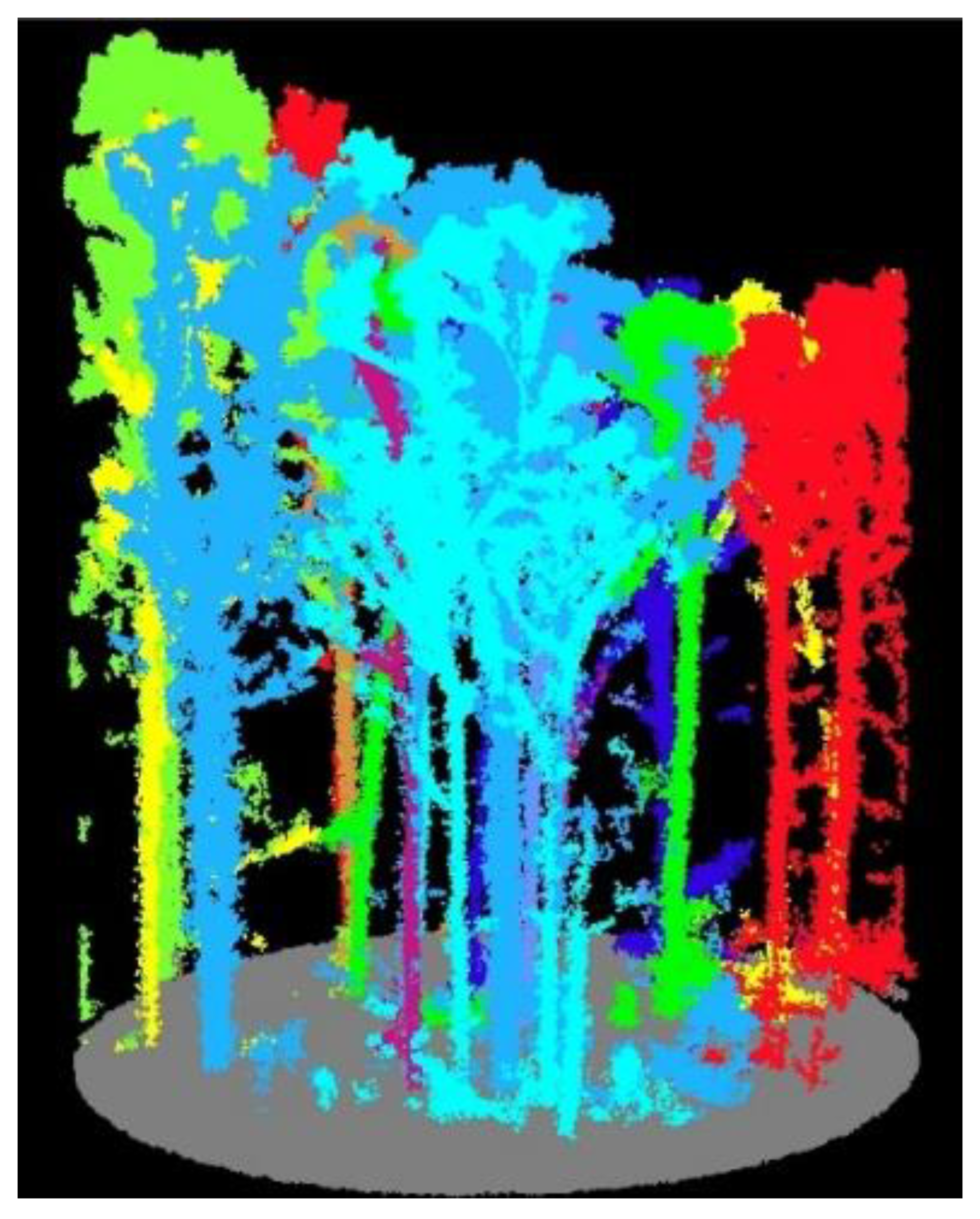
Subsequently, automatic segmentation of vegetation into individual trees, shrubs, and other categories was performed (
Figure 7).
All the aforementioned processing stages had to be carefully reviewed (visually) and any anomalies corrected to ensure the most accurate measurement of the segmented trees.
Since the measurements in the field and on the images were conducted on the same grid, which covers the selected stands, the plots and trees measured in the field could generally be found and linked with the measurements on the images. The data obtained from the image measurements were entered into the GIS database and merged with the field measurement data from the same plots for statistical processing, analysis, and modeling.
The data obtained through remote sensing methods (LiDAR) were compared at the plot sample level. The comparison included an evaluation of the accuracy of each estimated parameter, as well as the temporal dimension of the estimated data.
Therefore, for the observed variables (tree count, breast height diameter, height, basal area, volume) measured using different methods, statistical analysis was conducted (descriptive statistics and T-tests [
47]).
After the measurements were conducted on circular plots within individual compartments and age classes, comparisons between field measurements and measurements from the recordings for the same plots were made, and the accuracy was determined. Subsequently, further measurements were carried out at the level of larger areas (1 ha) and entire compartments (the principle of scaling from small to large).
LiDAR images were extracted using regular 1 ha plots (rectangular), which, like the circular plots, were randomly distributed within the compartments. Since field and recording measurements were conducted using the same sample grid, which covered the selected stands, plots, and trees measured within these plots, several 1 ha plots were distributed within the same compartments in the systematic sampling grid (100 x 100 m), in order to capture as much variability as possible within the compartment.
Each loaded plot (1 ha) underwent point cloud processing procedures, similar to the circular plots. Unlike the measurements on circular plots, where manual processing was present to a lesser or greater extent, in this case, the focus was on obtaining measurement data of satisfactory accuracy on larger areas through exclusively automatic processing. After the measurements on the 1 ha plots, the next step was the automatic measurement of segmented trees across the entire compartment.
3. Results
Since the research is based on developing a methodology for assessing structural parameters in operational forest inventory using LiDAR imagery, the analyses were conducted with the aim of contributing to a better (more detailed) interpretation of the observed advantages and/or disadvantages of the applied methodology. Specifically, the goal was to determine whether there is a difference between the field measurements and the LiDAR-based measurements, the magnitude of this difference, and whether it is statistically and operationally significant.
Therefore, for the comparison of field measurements and measurements from imagery (LiDAR), the data (tree species, height, breast height diameter, volume) were grouped into age classes, as it was expected that difficulties might arise in younger stands (age classes II and III). Namely, when creating the random sample, a condition was set for the representation of all age classes. Since the measurements in the field and from the imagery were conducted on the same sample grid, which covers the selected stands, plots, and trees measured on those plots, a consolidated database was created based on age classes.
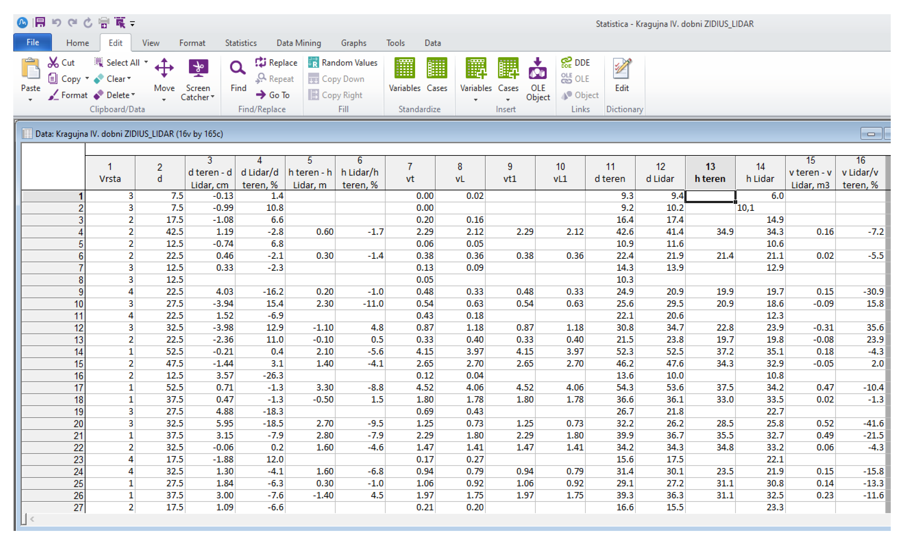
For the research area, based on measurements on 16 plots and 304 trees, the database was created for four age classes (IV, V, VI, VII), meaning that for these four age classes, it was possible to compare the same measured parameters in the field and from the imagery (
Figure 9). Based on this prepared database, T-tests were performed (
Table 1).
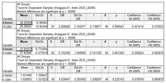
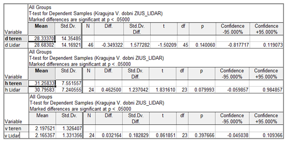
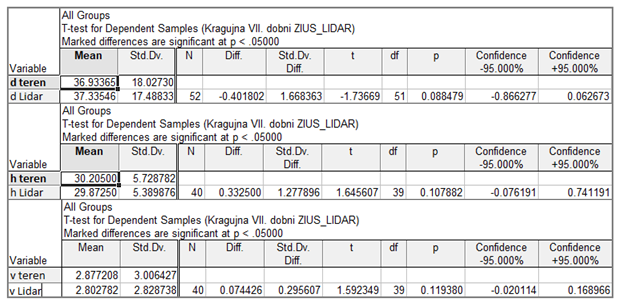
The results of the conducted T-test showed that in Age Class IV, there is no statistically significant difference between the diameters and heights measured in the field and from the LiDAR imagery. Accordingly, there is also no significant difference in the calculated volume between the field measurements and LiDAR imagery (
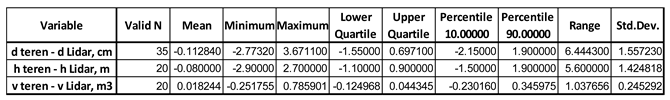
Table 1). The results of the descriptive statistics (in this case for Age Class IV) are presented in
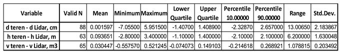
Table 2.
Table 2 shows that the mean deviations (Mean) for all variables (d (DBH), h, v) are negligible (almost identical), which was also the research hypothesis.
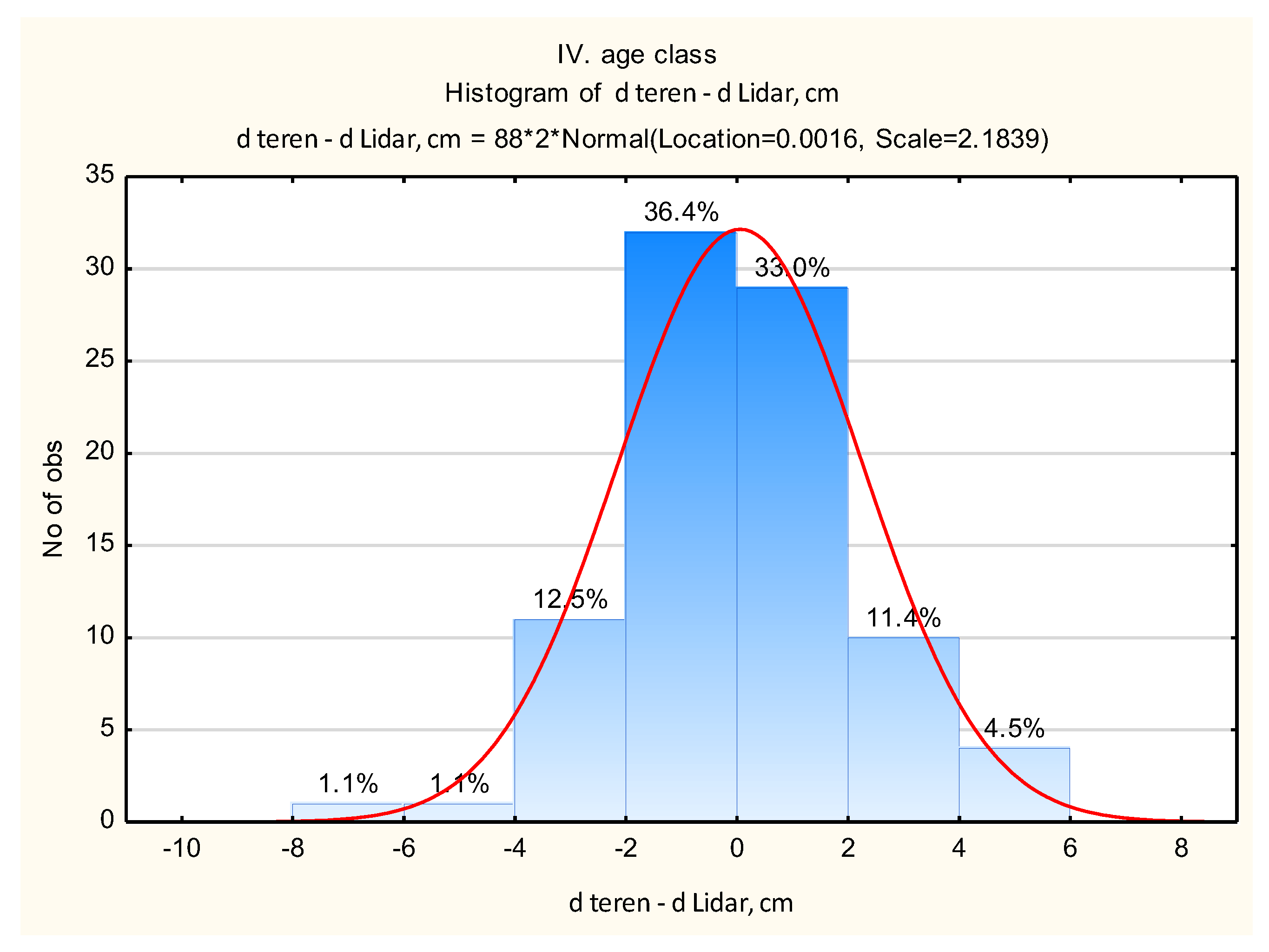
In addition to the range of deviations in specific percentiles, we are also interested in the percentage share of deviations within certain classes. The obtained results can be presented and interpreted using a histogram (
Figure 10).
Thus, the histogram (
Figure 10) shows that approximately 70% of the deviations in breast height diameters fall within +/- 2 cm.
Additionally, the histogram reveals the percentage of trees within the IV age class that exhibit maximum deviations in breast height diameter, and it also identifies the specific trees in question. These include two hornbeam trees (19 and 20) and two trees of other species (9 and 138), for which the breast height diameter measured in the field was larger than that recorded in the LiDAR images.
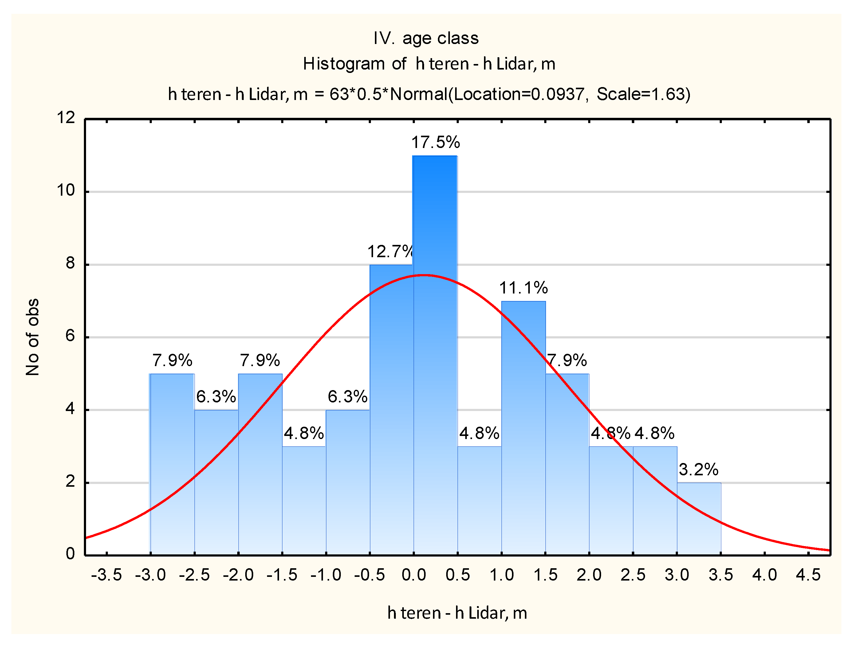
Based on the histogram of height deviations measured in the field and on the LiDAR images, it can be observed that 7.9% of the heights deviate within the range of -3 to -2 m (
Figure 11). This category includes 5 trees for which a greater height was measured on the LiDAR images than in the field.
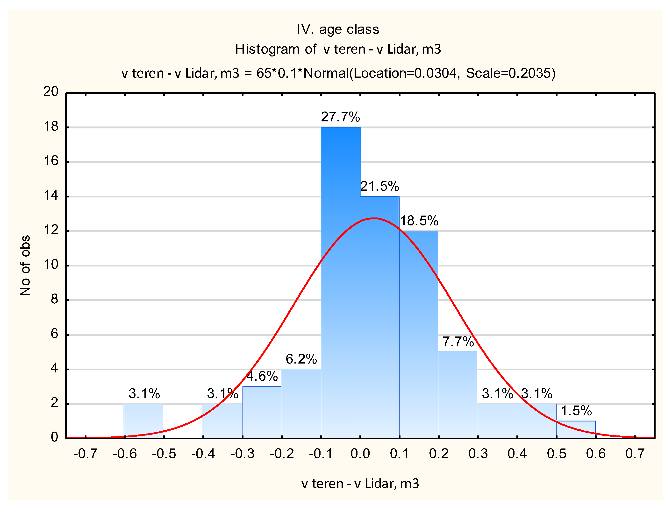
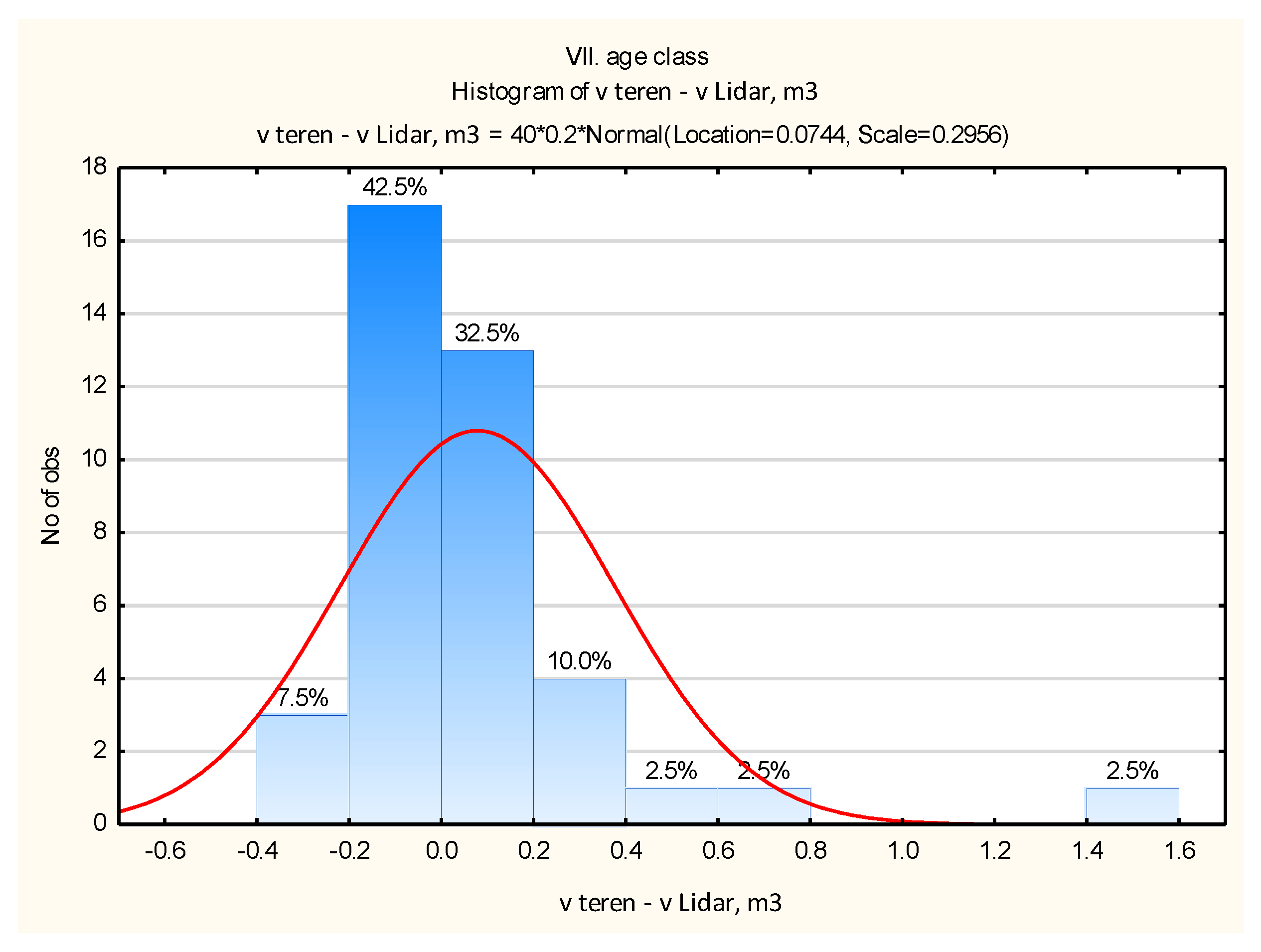
Regarding the volume, as shown in
Figure 12, the distribution of deviations is uniform, and the results of descriptive statistics indicate that the mean deviations are negligible.
For the V. age class, a consolidated database was created, based on which T-tests were performed (
Table 3).
The results of the T-tests show that there is no statistically significant difference for the tested variables (diameter at breast height (DBH), height (h), and volume(v)) measured in the field and on the images (
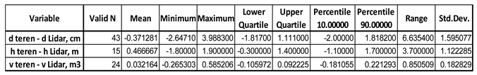
Table 3). The results of the descriptive statistics are presented in
Table 4.
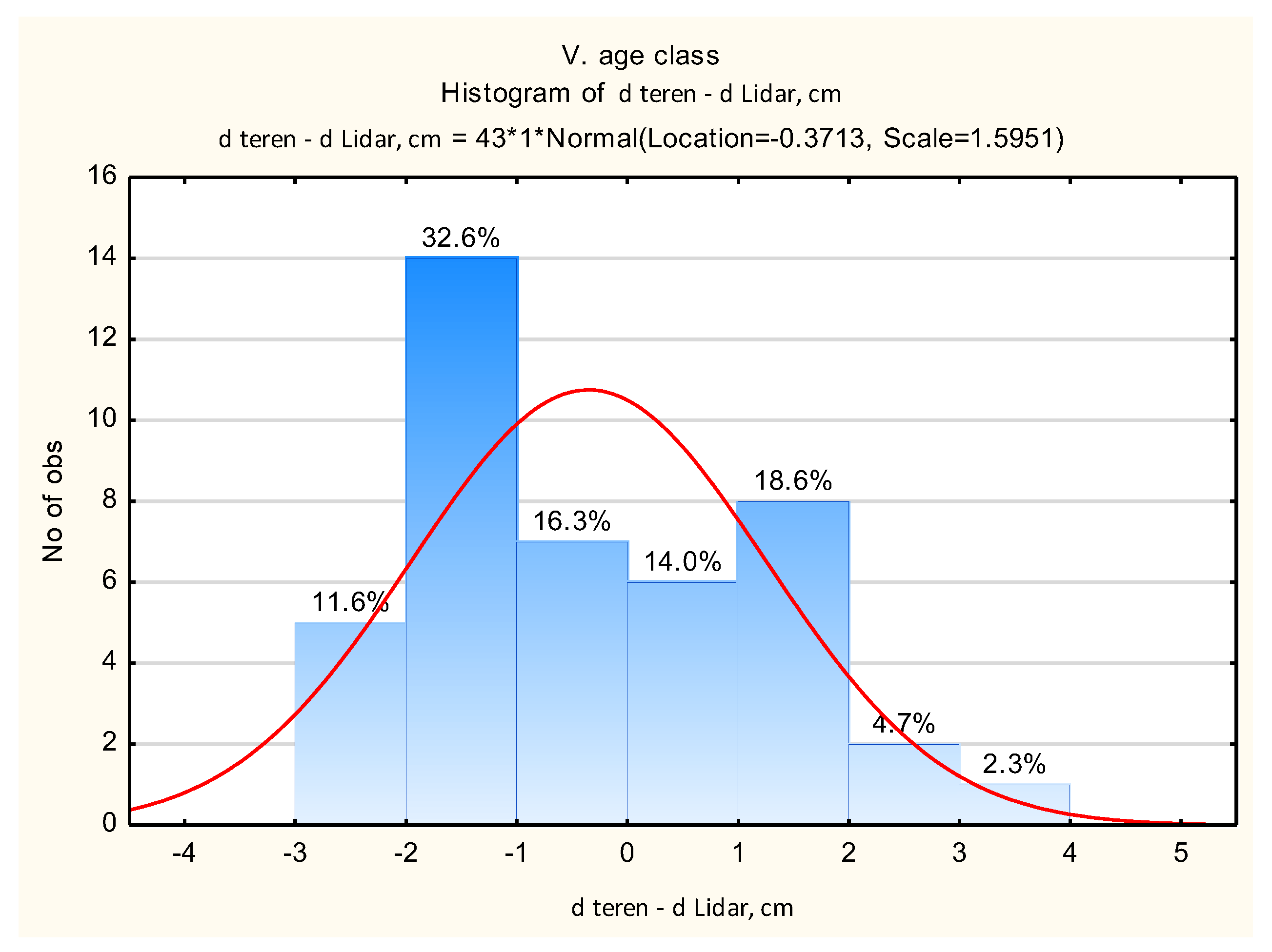
The results of the descriptive statistics for the V age class show that in 80% of cases, the deviation in breast height diameter ranges from -2 to 1.8 cm. Differences in heights exist (Mean), but they are not statistically significant. Larger diameter values on LiDAR and smaller heights result in almost no difference in volumes.
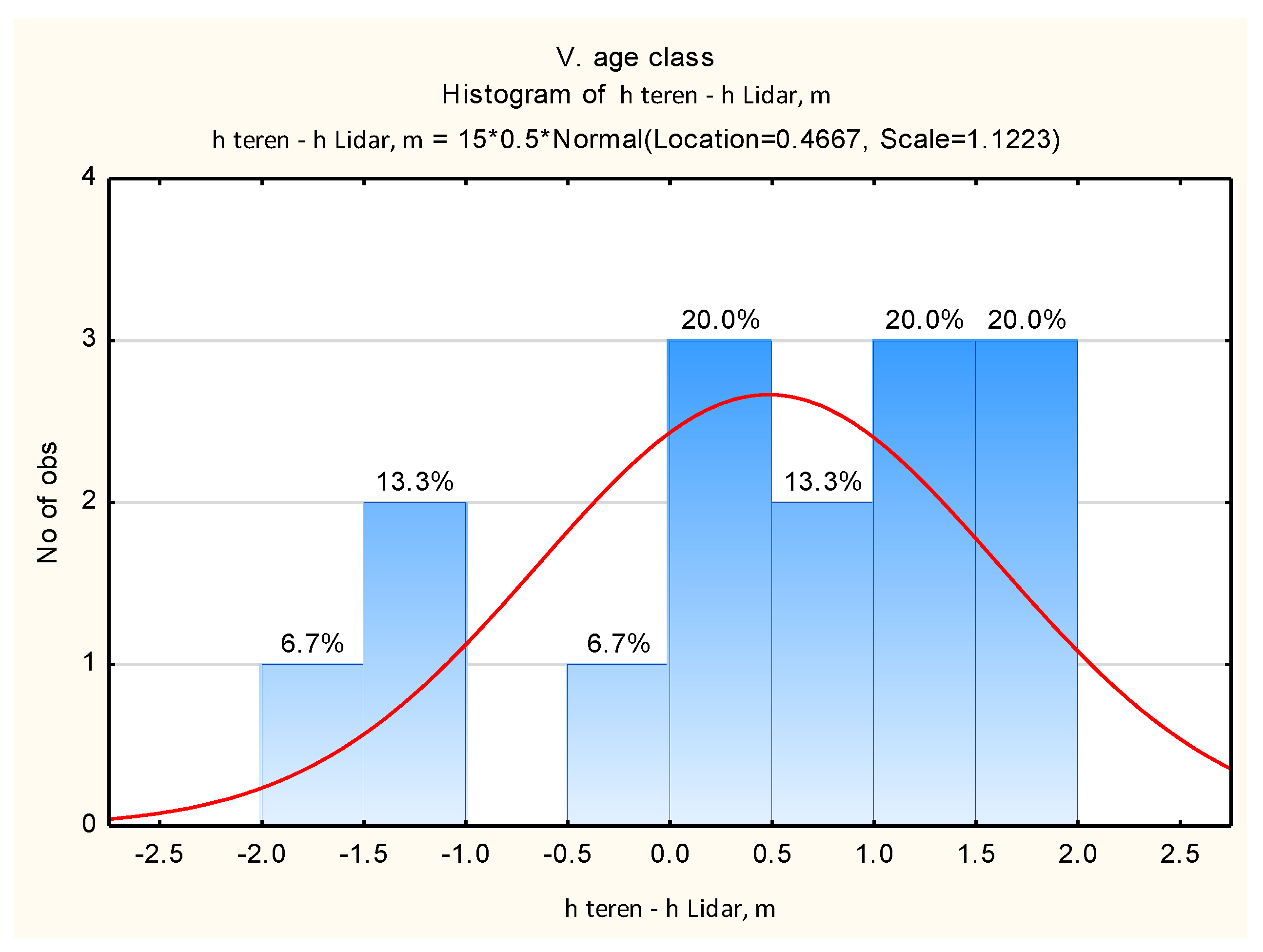
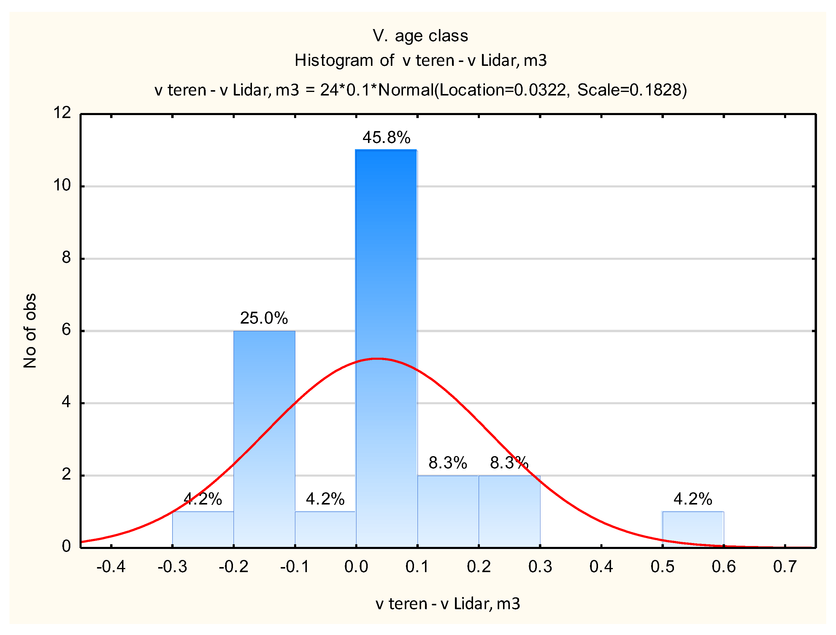
If we are interested in the percentage distribution of deviations within certain classes, or in identifying which trees are involved in each category, the obtained results can be presented using a histogram (
Figure 13,
Figure 14 and
Figure 15).
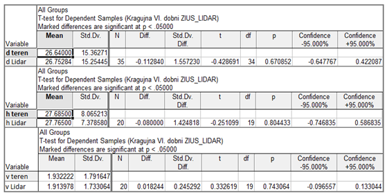
For the VI. age class, a consolidated database was also created, and T-tests were conducted (
Table 5), which confirm that there is no statistically significant difference between the diameters and heights measured in the field and those obtained from LiDAR scans. Consequently, no significant difference was found in the calculated volume between the field measurements and those from the LiDAR scans (
Table 6).
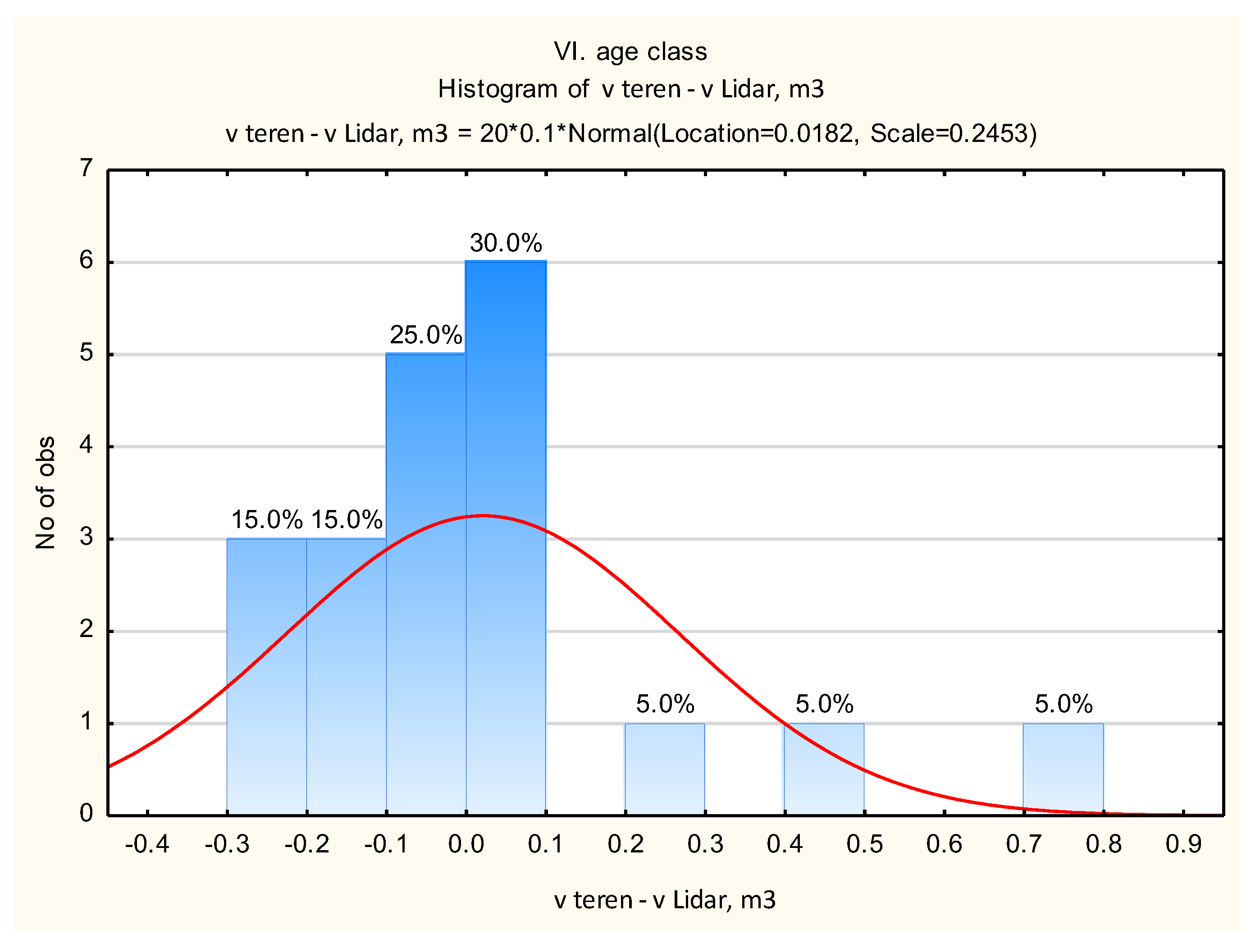
The results of descriptive statistics show that the mean deviations (Mean) for all variables (d (DBH), h, v) are negligible, and that in 80% of cases, for example, the volume deviation ranges from -0.23 to +0.35 m³.
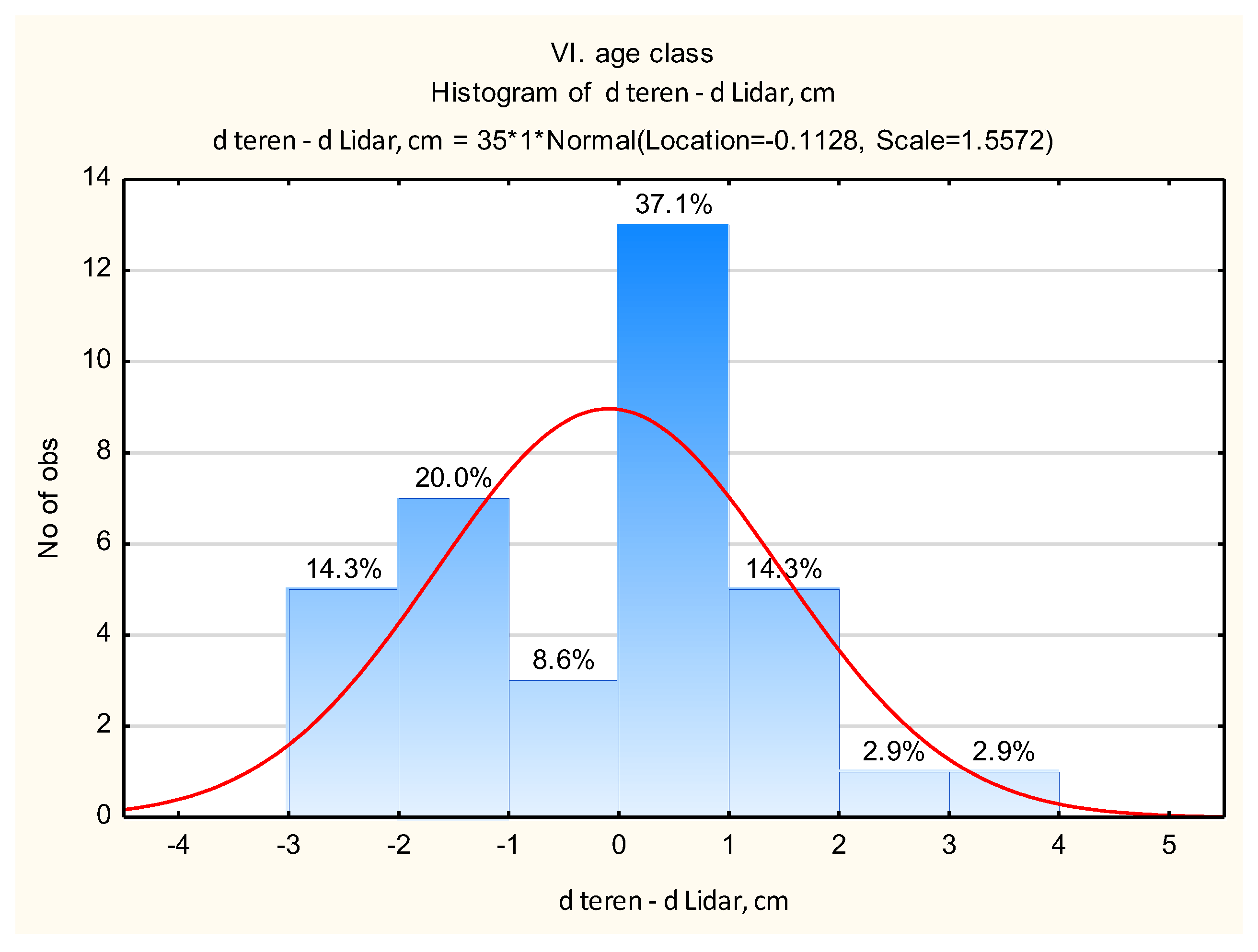
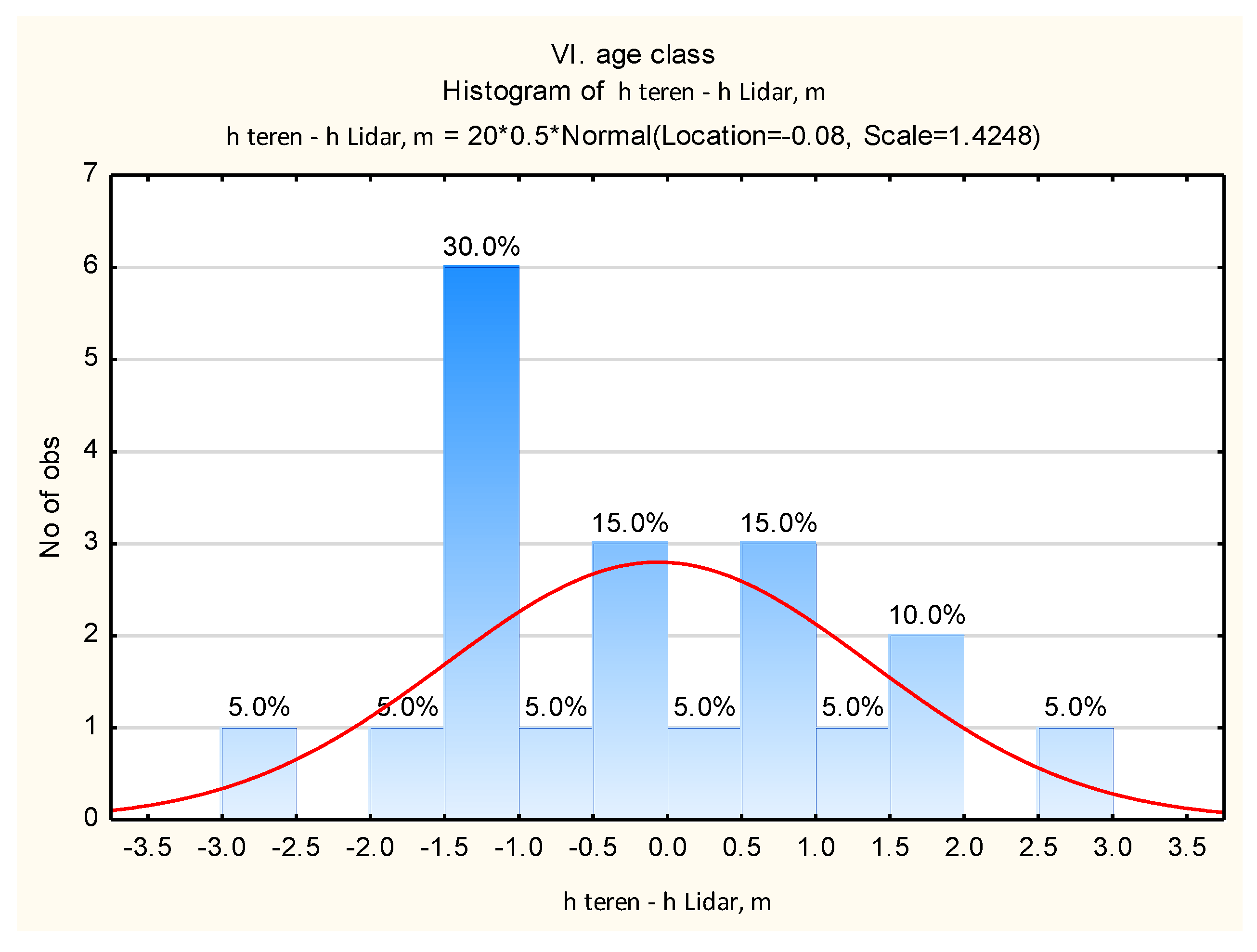
Also, if we are interested in the percentage distribution of deviations within certain classes, or in identifying which trees are involved in each category, the obtained results can be presented using a histogram (
Figure 16,
Figure 17 and
Figure 18).
For the VII age class, a consolidated database was also created, and T-tests were performed (
Table 7), which confirm that there is no statistically significant difference between the diameters and heights measured in the field and on LiDAR imagery. Consequently, there is no significant difference in the calculated volume between the field measurements and those obtained from LiDAR imagery (
Table 8).
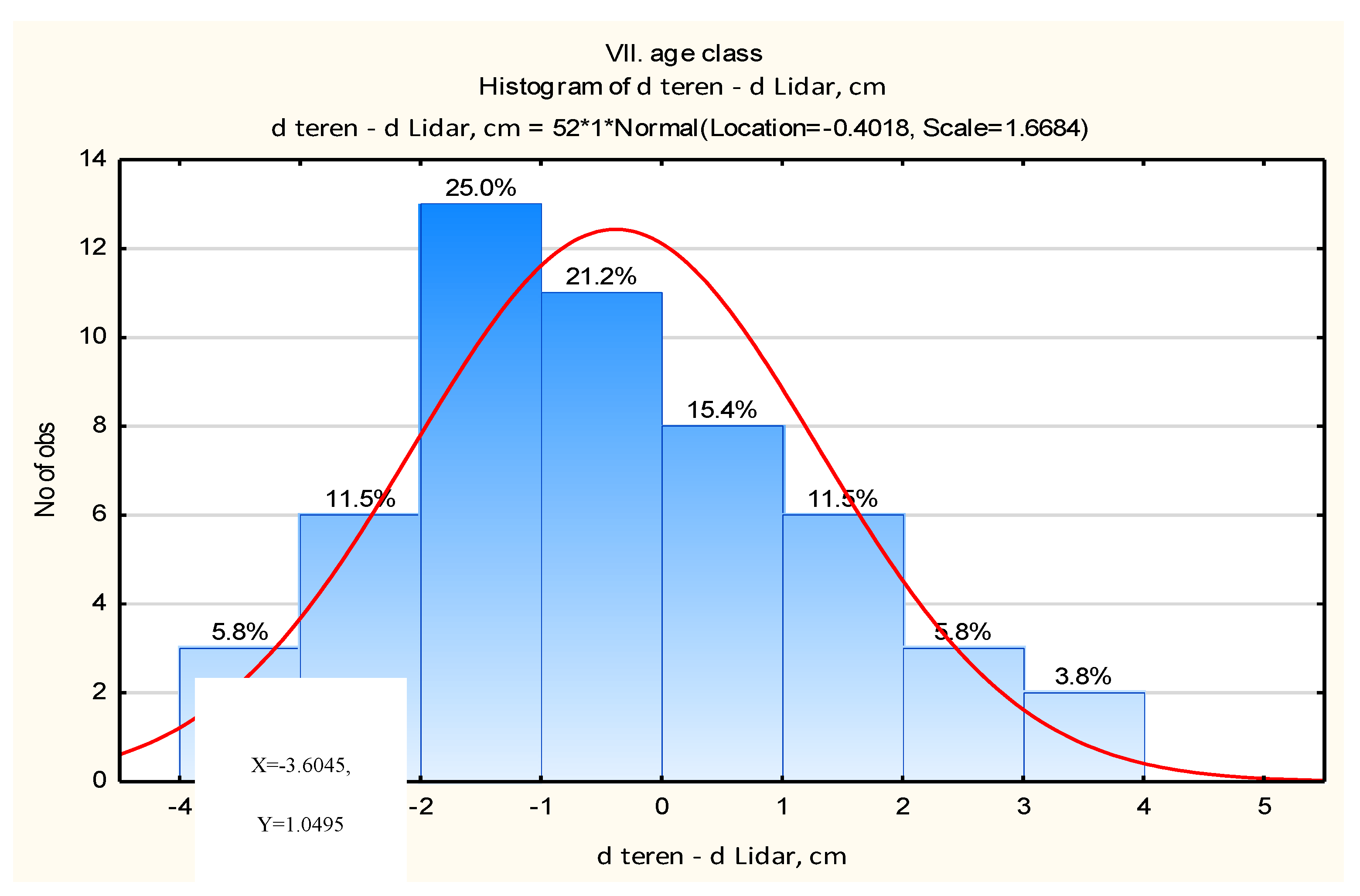
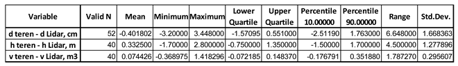
The results of the descriptive statistics show that the mean deviations (Mean) for all variables (d (DBH), h, v) are negligible, and in 80% of cases, for example, the range for volume is from -0.23 to +0.35 m³. Differences in height are present (Mean), but they are not statistically significant.
Based on the histogram (
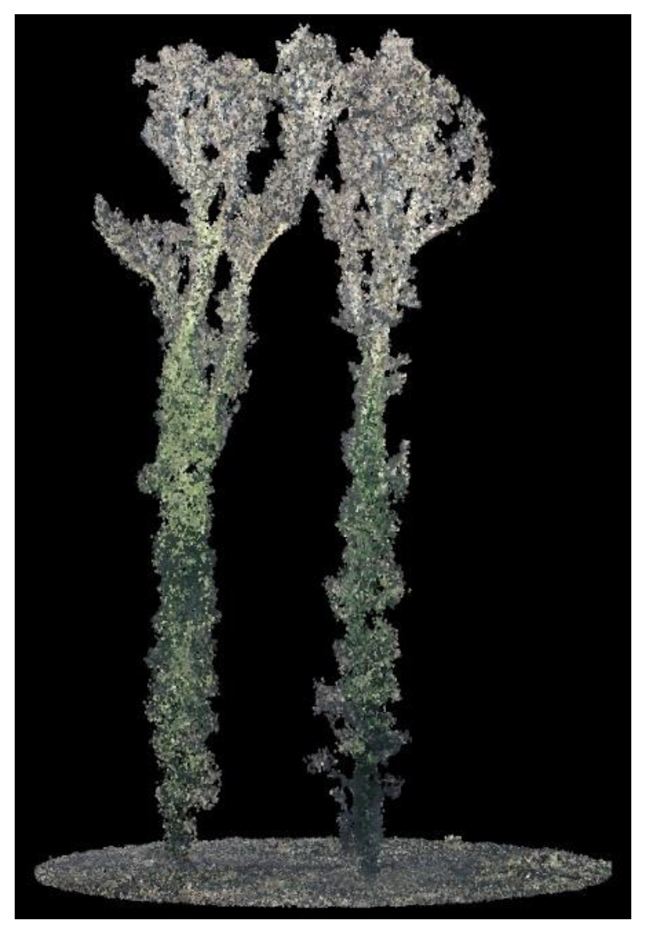
Figure 19) displaying the deviations in breast heights measured in the field and from the LiDAR images, it can be seen that 11.5% of the breast height measurements fall within the range of -3 to -2 cm, while 17% exceed 2 cm. This category includes three trees (77, 89, and 91), for which a larger breast height was measured on the LiDAR images compared to the field measurements.
Since the histogram shows which trees had a larger diameter at breast height (DBH) measured in the LiDAR images, by reviewing the database, we can identify the plot in question and observe what these trees look like in the images (
Figure 20).
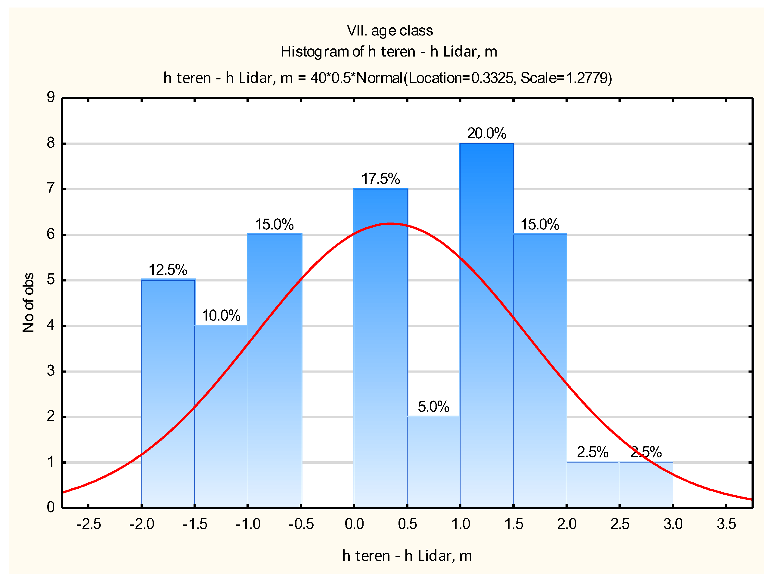
The results from the histograms (
Figure 21 and
Figure 22) facilitate the identification of larger deviations and their overall distribution, allowing for the determination of the reasons behind the discrepancies.
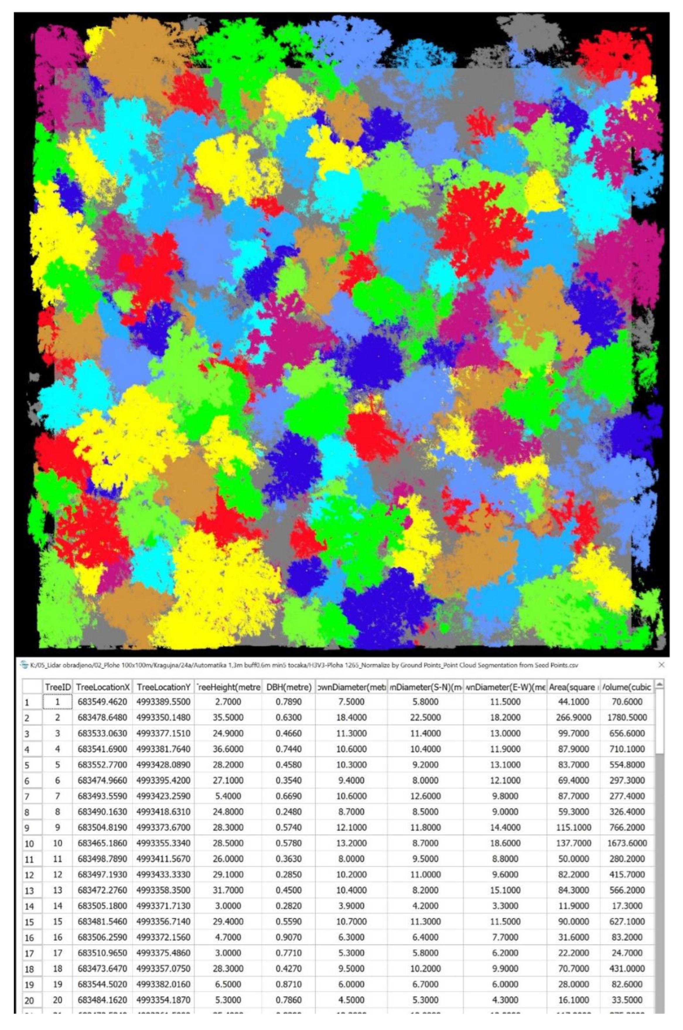
On the 1 ha plots, the following results for diameter at breast height, tree height, crown width, and other parameters were obtained through automatic measurement of the LiDAR images (
Figure 23).
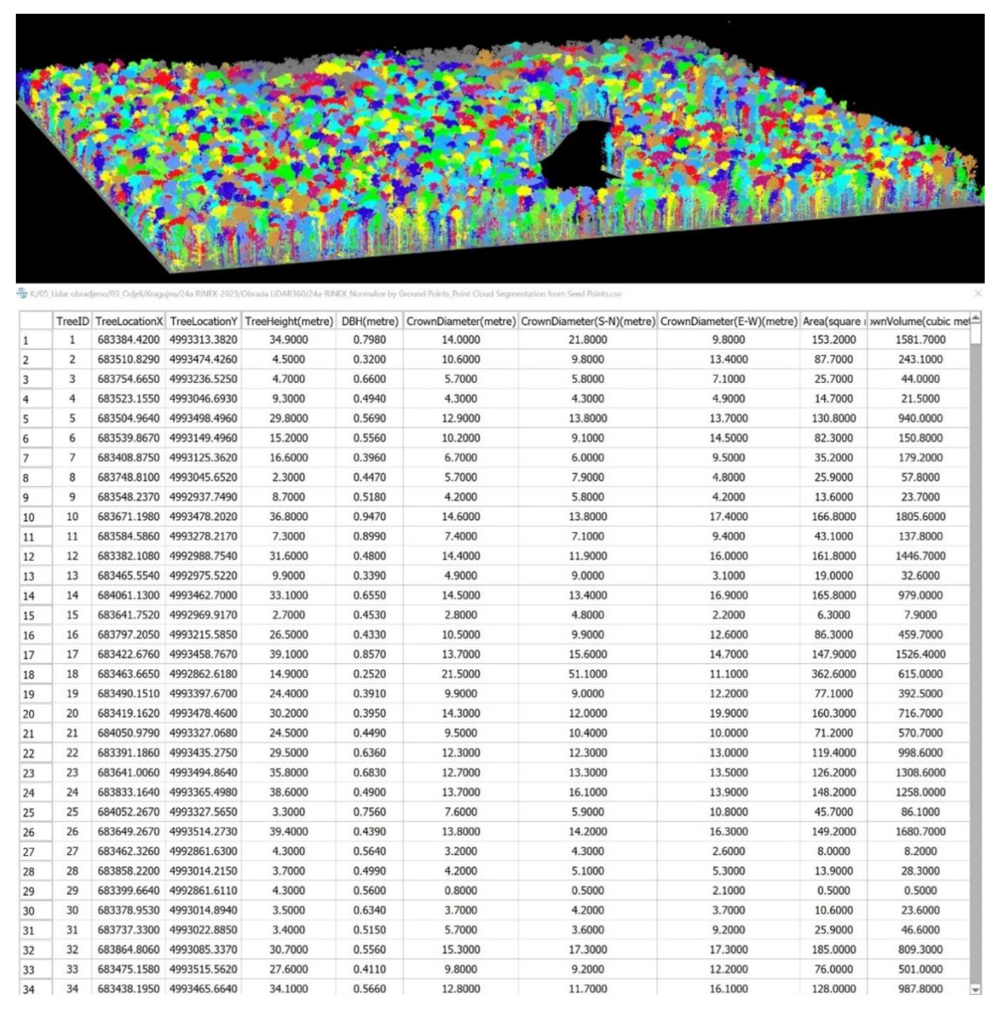
In subcompartment 24a (51 ha), a total of 12 172 trees were extracted through automatic processing (
Figure 24).
The summary results of the automatic processing of tree numbers and breast height diameter are presented for 1-hectare plots and for the entire compartment (
Table 9). It is evident from
Table 9 that the mean breast height diameter and the number of trees per hectare on the random 1-hectare plots differ only slightly from the same parameters measured for the entire compartment and recalculated per hectare.
It is important to note that, in addition to automated processing, manual processing of the scans was also applied to the circular surfaces, which certainly further affects the accuracy of the measurements of the circular surfaces. Based on the results of the analyses conducted on the circular surfaces, it was determined that, in most cases, the breast diameters are overestimated, while the tree heights are underestimated. However, this may not necessarily have a significant impact on the volume.
4. Discussion
Based on all the presented results for the IV, V, VI, and VII age classes, it was determined that there is no statistically significant difference between the diameters and heights measured on the ground and those measured from LiDAR imagery, and consequently, no difference in the calculated volume. The obtained results were confirmed through T-tests, and the results of descriptive statistics support this, showing that the mean deviations for the examined variables (d (DBH), h, v) are negligible.
The obtained results were also presented in histograms to more easily identify deviations, determine the percentage share of each class of deviation, and potentially identify the cause of the deviation (especially for classes with significant deviations). Specifically, in the VII age class, in one case, a larger diameter was measured on certain trees in the LiDAR imagery. Analysis of these trees in the imagery (
Figure 20) revealed that the cause was ivy. Smaller diameters were measured on the LiDAR imagery in the IV age class, but in this case, the trees in question were two hornbeams and two trees of other species. The reason for this is the low number of points in the point cloud and the inability to precisely measure the breast height diameter on imagery for thin trees.
Finally, an analysis of the operational applicability of LiDAR imagery for estimating the number of trees, basal area, and volume, by diameter classes and overall, was conducted. Taking volume as an example, which is of the most operational interest, based on the obtained results, it can be concluded that there is no difference between the ground measurements and the LiDAR imagery for oak and ash trees. However, the difference is mainly found in the lower diameter classes for hornbeam and other tree species. These differences are not caused by the tree species, but by the dimensions of the trees. In lower age classes, the average volume obtained from LiDAR is lower, ranging from -0.08% to -0.86%.
When it comes to the automatic processing of LiDAR scans, it is important to highlight the issue of younger stands (age classes II and III), for which it was not possible to determine the forestry parameters from the scans. This is confirmed by the research conducted by Windrim et al [
48]. The same problem was encountered with circular surfaces, where manual processing was also introduced. In younger age classes (II and III), there is a higher number of thinner trees, and the stands are denser, which poses a significant challenge for automatic processing. Additionally, it was shown that even manual processing did not significantly contribute to the accuracy of the obtained results on the circular surfaces. Consequently, automatic measurements can be used for operational purposes (quick screening), but with the limitations mentioned above in mind.
Remaining are the stands of age class I, for which the same considerations as previously mentioned apply. However, the determination of forestry parameters is not expected due to the high tree density, as noted by Wang et al [
49]. Nevertheless, through automatic processing, it is possible to obtain data that are important from the perspective of generating a basis for biomass estimation over larger areas.
This study demonstrated that a minimum of three passes over the same area are required to ensure that trees are scanned from all sides, thereby obtaining a higher-quality point cloud and, consequently, a more precise measurement of parameters, primarily breast height diameters. It is recommended that the scanning be carried out in winter, during the period when measurements are taken as part of the regular forest inventory, as this is when vegetation is dormant and trees are leafless. This condition facilitates better scan processing and the determination of forestry parameters, as also noted by Coops et al. [
4] in their research.
The results of this study have shown that remote sensing is a valuable source of information and can be applied in operational forest management, supporting the research conducted by Wulder et al [
12]. Accordingly, reliable and efficient measurement of forestry parameters from LiDAR scans, along with the identification of tree species from RGB/CIR scans, can facilitate the development of stand height curves as demonstrated in the study by Chen et al [
50]. Additionally, it can assist in stand classification and, with further development of the methodology, contribute to the delineation of forest stands (subcompartments).
Furthermore, the proven advantages of remote sensing methods should be leveraged, particularly in terms of significant rationalization of field measurements while obtaining equally reliable data and substantially reducing costs, as confirmed by several studies [
2,
9,
10,
11].
5. Conclusions
Based on all the presented results for the study area, we can conclude that there is no statistically significant difference between the diameters and heights measured in the field and those measured from LiDAR imagery, and consequently, no significant difference in the calculated volume for the IV, V, VI, and VII age classes, as confirmed by the T-tests. This is further supported by the results of the descriptive statistics, which show that the mean deviations for the tested variables (d (DBH), h, v) are negligible.
During the research, numerous advantages of applying remote sensing methods (RS) compared to traditional field measurements were observed, but some drawbacks were also identified, which can be addressed. Some of these relate to the recording procedures (such as time, season, etc.), while others concern the preprocessing of the imagery, the appropriate software support, and so on. The experiences and results from this project will serve as a basis for the standardization of such research in other areas.
Since unmanned aerial vehicle imagery (with various sensors) is increasingly used in everyday forestry operations, its application does not eliminate fieldwork but can significantly reduce it while achieving the same level of accuracy in the results. As a result, this approach can lead to substantial savings in both time and costs.
Author Contributions
Conceptualization, J. K. and R. P.; methodology, R. P.; software, M. A.; validation, R.P., M.A. and A.S.; formal analysis, J. K. and R. P.; investigation, J.K, R.P., A.S, and M.A.; data curation, J.K.; writing—original draft preparation, R. P.; writing—review and editing, J. K., A. S. and M. A.; visualization, J.K. and M.A.; supervision, R.P. All authors have read and agreed to the published version of the manuscript. All authors have read and agreed to the published version of the manuscript.
Funding
The research was carried out in the Laboratory for remote sensing and GIS, Faculty of Forestry and Wood Technology. Thanks to the University of Zagreb, Faculty of Forestry and Wood Technology, for the support and funding of the research.
Data Availability Statement
The data presented in this study are available on request from the corresponding author.
Acknowledgments
We would like to express our gratitude to the company Hrvatske šume d.o.o. for providing the financial support for this research.
Conflicts of Interest
The authors declare no conflict of interest.
References
- Næsset, E. Area-based inventory in Norway – from innovation to an operational reality. In For Appl Airborne Laser Scanning Concepts Case Stud; Maltamo, M., Næsset, E., Vauhkonen, J., Eds.; Springer: Netherlands, Dordrecht, 2014; pp. 215–240. [Google Scholar]
- White, J. C.; Coops, N. C.; Wulder, M. A.; Vastaranta, M.; Hilker, T.; Tompalski, P. Remote sensing technologies for enhancing forest inventories: A review. Canadian Journal of Remote Sensing 2016, 42, 619–641. [Google Scholar] [CrossRef]
- Magnussen, S.; Nord-Larsen, T.; Riis-Nielsen, T. Lidar supported estimators of wood volume and above ground biomass from the Danish national forest inventory (2012–2016). Remote Sens. Environ. 2018, 211, 146–153. [Google Scholar] [CrossRef]
- Coops, C.; Tompalski, P.; Goodbody, T. R.H.; Queinnec, M.; Luther, J. E.; Bolton, D. K.; White, J. C.; Wulder, M.A.; R. van Lier, O.; Hermosilla, T. Modelling lidar-derived estimates of forest attributes over space and time: A review of approaches and future trends Nicholas. Remote Sensing of Environment 2021, 260, 112477. [Google Scholar] [CrossRef]
- Pranjić, A.; Lukić, N. Izmjera šuma. Šumarski fakultet, Sveučilište u Zagrebu, 1997, 405 str., Zagreb.
- Arslan, A.E.; İnan, M.; Çelik, M.F.; Erten, E. Estimations of Forest Stand Parameters in Open Forest Stand Using Point Cloud Data from Terrestrial Laser Scanning, Unmanned Aerial Vehicle and Aerial LiDAR Data. European Journal of Forest Engineering 2022, 8, 46–54. [Google Scholar] [CrossRef]
- Bodaghi, M.; Kránitz, J.; Jung, A. UAV LIDAR IMAGING BASED FOREST MAPPING. In Proceedings of the Vol. 2, 8th International Conference on Cartography and GIS, Nessebar, Bulgaria, 20–25 June 2022; Bandrova, T., Konečný, M., Marinova, S., Eds.; 1314. ISBN 1314-0604. [Google Scholar]
- Janiec, P.; Hawryło, P.; Tymińska-Czabańska, L.; Miszczyszyn, J.; Socha, J. A low-cost alternative to LiDAR for site index models: applying repeated digital aerial photogrammetry data in the modelling of forest top height growth. Forestry: An International Journal of Forest Research 2024. [Google Scholar] [CrossRef]
- Pernar, R.; Šelendić, D. Prilog povećanju interpretabilnosti aerosnimaka i satelitskih snimaka za potrebe uređivanja šuma. Glasnik za šumske pokuse 2006, 5, 467–477. [Google Scholar]
- Valbuena, R.; Maltamo, M.; Packalen, P. Classification of multilayered forest development classes from low-density national airborne lidar datasets. Forestry: An International Journal of Forest Research 2016, 89, 392–401. [Google Scholar] [CrossRef]
- Pernar, R.; Ančić, M.; Seletković, A.; Kolić, J. Važnost daljinskih istraživanja pri procjeni šteta na šumskim sastojinama uzrokovanih velikim prirodnim nepogodama. Proceedings of Gospodarenje šumama u uvjetima klimatskih promjena i prirodnih nepogoda, Zagreb, Croatia, 20.04.2018.; Anić, Igor; Publisher: HAZU, Zagreb, Croatia, 2020; pp. 143–160. [Google Scholar] [CrossRef]
- Wulder, M.A.; Hermosilla, T.; White, J.C.; Coops, N.C. Biomass status and dynamics over Canada’s forests: disentangling disturbed area from associated aboveground biomass consequences. Environ. Res. Lett. 2020, 15, 094093. [Google Scholar] [CrossRef]
- Benko, M.; Balenović, I. PROŠLOST, SADAŠNJOST I BUDUĆNOST PRIMJENE METODA DALJINSKIH ISTRAŽIVANJA PRI INVENTURI ŠUMA U HRVATSKOJ. Šumarski list – Posebni broj 2011, 272–281. [Google Scholar]
- Gajski, D. Osnove laserskog skeniranja iz zraka. Ekscentar [Internet] 2007, 10, 16–22. [Google Scholar]
- Nelson, R. How did we get here? An early history of forestry lidar. Can. J. Remote. Sens. 2013, 39 (Suppl. 1), S6–S17. [Google Scholar] [CrossRef]
- Mitchum, J. Evaluation of Airborne Lidar to Estimate Tree Height in a Dense Forest Canopy. 2018. [Google Scholar]
- Lefsky, M.A.; Cohen, W. B.; Acker, S. A.; Spies, T.A.; Parker, G.G.; Harding, D. Lidar remote sensing of biophysical properties and canopy structure of forest of Douglas-fir and western hemlock. Remote Sens. Environ. 1999, 70, 339–361. [Google Scholar] [CrossRef]
- Zimble, D.A.; Evans, D.L.; Carlson, G.C.; Parker, R.C.; Grado, S.C.; Gerard, P.D. Characterizing vertical forest structure using small-footprint airborne LiDAR. Remote Sens. Environ. 2003, 87, 171–182. [Google Scholar] [CrossRef]
- Hall, S.A.; Burke, I.C.; Box, D.O.; Kaufmann, M.R.; Stoker, J.M. Estimating stand structure using discrete-return lidar: an example from low density, fire prone ponderosa pine forests. For. Ecol. Manage. 2005, 208, 189–209. [Google Scholar] [CrossRef]
- Maltamo, M.; Packalen, P.; Yu, X.; Eerikainen, K.; Hyyppa, J.; Pitkanen, J. Identifying and quantifying structural characteristics of heterogeneous boreal forests using laser scanner data. For. Ecol. Manage. 2005, 216, 41–50. [Google Scholar] [CrossRef]
- Reutebuch, S.E.; Andersen, H.-E.; McGaughey, R.J. Light detection and ranging (LIDAR):an emerging tool for multiple resource inventory. J Forestry. 2005, 103, 286–292. [Google Scholar] [CrossRef]
- Kellner, J. R.; Asner, G. P. Convergent structural responses of tropical forests to diverse disturbance regimes. Ecol. Lett. 2009, 12, 887–897. [Google Scholar] [CrossRef] [PubMed]
- Jaskierniak, D.; Lane, P. N. J.; Robinson, A.; Lucieer, A. Extracting LiDAR indices to characterise multilayered forest structure using mixture distribution functions. Remote Sens. Environ. 2011, 115, 573–585. [Google Scholar] [CrossRef]
- Ussyshkin, V.; Theriault, L. Airborne lidar: advances in discrete return technology for 3D vegetation mapping. Remote Sensing 2011, 3, 416–434. [Google Scholar] [CrossRef]
- Valbuena, R.; Packalen, P.; Mehta¨talo, L.; Garcı ´a-Abril, A.; Maltamo, M. Characterizing forest structural types and shelterwood dynamics from Lorenz-based indicators predicted by airborne laser scanning. Can. J. For. Res. 2013, 43, 1063–1074. [Google Scholar] [CrossRef]
- Balestra, M.; Marselis, S.; Sankey, T.T.; et al. LiDAR Data Fusion to Improve Forest Attribute Estimates: A Review. Curr. For. Rep. 2024, 10, 281–297. [Google Scholar] [CrossRef]
- Rocha, K.D.; Silva, C.A.; Cosenza, D.N.; Mohan, M.; Klauberg, C.; Schlickmann, M.B.; Xia, J.; Leite, R.V.; Almeida, D.R.A.d.; Atkins, J.W.; et al. Crown-Level Structure and Fuel Load Characterization from Airborne and Terrestrial Laser Scanning in a Longleaf Pine (Pinus palustris Mill.) Forest Ecosystem. Remote Sens. 2023, 15, 1002. [Google Scholar] [CrossRef]
- Waser, L.; Day, R.; Chasmer, L.; Taylor, A. Influence of vegetation structure on Lidar-derived canopy height and fractional cover in forested riparian buffers during leaf-off and leaf-on conditions. PLoS One 2013, 8, e54776. [Google Scholar] [CrossRef]
- Balestra, M.; Tonelli, E.; Vitali, A.; Urbinati, C.; Frontoni, E.; Pierdicca, R. Geomatic Data Fusion for 3D Tree Modeling: The Case Study of Monumental Chestnut Trees. Remote Sens 2023. [Google Scholar] [CrossRef]
- Queinnec, M.; Coops, N. C.; White, J. C.; McCartney, G.; Sinclair, I. Developing a forest inventory approach using airborne single photon lidar data: from ground plot selection to forest attribute prediction. Forestry 2022, 95, 347–362. [Google Scholar] [CrossRef]
- Zhao Y, Im J, Zhen Z, Zhao Y. Towards accurate individual tree parameters estimation in dense forest: optimized coarse-to-fine algorithms for registering UAV and terrestrial LiDAR data. GIS-cience Remote Sens. 2023, 60, 2197281. [Google Scholar] [CrossRef]
- Luo, H.; Wang, C.; Wen, C.; Chen, Z.; Zai, D.; Yu, Y.; Li, J. Semantic Labeling of Mobile LiDAR Point Clouds via Active Learning aid Higher Order MRF. IEEE Transactions on Geoscience and Remote Sensing 2018, 56, 3631–3644. [Google Scholar] [CrossRef]
- Hauglin, M.; Rahlf, J.; Schumacher, J. Large scale mapping of forest attributes using heterogeneous sets of airborne laser scanning and National Forest Inventory data. For Ecosyst. 2021, 8, 1–15. [Google Scholar] [CrossRef]
- Hopkinson, C.; Chasmer, L.; Hall, R.J. The uncertainty in conifer plan tation growth prediction from multi-temporal lidar datasets. Remote Sens Environ. 2008, 112, 1168–80. [Google Scholar] [CrossRef]
- Socha, J.; Hawryło, P.; Sterenczak, K. Assessing the sensitivity of site index models developed using bi-temporal airborne laser scanning data to different top height estimates and grid cell sizes. Int J Appl Earth Observ Geoinform. 2020, 91, 102129. [Google Scholar] [CrossRef]
- Tyminska-Czabanska, L.; Socha, J.; Hawryło, P. Weather-sensitive height growth modelling of Norway spruce using repeated airborne laser scanning data. Agric For Meteorol. 2021, 308, 108568. [Google Scholar] [CrossRef]
- Tymińska-Czabanska, L.; Hawryło, P.; Socha, J. Assessment of the effect of stand density on the height growth of scots pine using repeated ALS data. Int J Appl Earth Observ Geoinform. 2022, 108, 102763. [Google Scholar] [CrossRef]
- Burger, J.A. Management effects on growth, production and sustainability of managed forest ecosystems: past trends and future directions. For. Ecol. Manage 2009, 258, 2335–2346. [Google Scholar] [CrossRef]
- Packalen, P.; Heinonen, T.; Pukkala, T.; Vauhkonen, J.; Maltamo, M. Dynamic treatment units in eucalyptus plantation. For. Sci. 2011, 57, 416–426. [Google Scholar] [CrossRef]
- Slavík, M.; Kuželka, K.; Modlinger, R.; Surový, P. Spatial Analysis of Dense LiDAR Point Clouds for Tree Species Group Classification Using Individual Tree Metrics. Forests 2023, 14, 1581. [Google Scholar] [CrossRef]
- Koc-San, D.; Selim, S.; Aslan, N.; San, B.T. Automatic citrus tree extraction from UAV images and digital surface models using circular Hough transform. Computers and Electronics in Agriculture 2018, 150, 150,289–301. [Google Scholar] [CrossRef]
- Demir, N. Using UAVs for detection of trees from digital surface models. Journal of Forestry Research 2018, 29, 813–821. [Google Scholar] [CrossRef]
- Liang, X.; Wang, Y.; Pyorala, J.; Lehtomaki, M.; Yu, X.; Kaartinen, H.; Kukko, A.; Honkavaara, E.; Issao ui, A.E.I.; Nevalainen, O. Forest in situ observations using unmanned aerial vehicle as an alternative of terrestrial measurements. Forest Ecosystems. 2019, 6, 20. [Google Scholar] [CrossRef]
- Guerra-Hernandez, J.; Diaz-Varela, R.A.; Avarez- Gonzalez, J.G.; Rodriguez-Gonzalez, P.M. Assessing a novel modelling approach with high resolution UAV imagery for monitoring health status in priority riparian forests. Forest Ecosystems 2021, 8, 61. [Google Scholar] [CrossRef]
- Goodbody, T.R.H.; Coops, N.C.; Marshall, P.L.; Tompalski, P.; Crawford, P. Unmanned aerial systems for precision forest inventory purposes: a review and case study. For. Chron. 2017, 93, 71–81. [Google Scholar] [CrossRef]
- Popescu, S. Estimating biomass of individual pine trees using air-borne LIDAR. Biomass and Bioenergy 2007, 31, 646–655. [Google Scholar] [CrossRef]
- Jazbec, A. 2008: Osnove statistike. Šumarski fakultet, Zagreb, 136 str.
- Windrim, L.; Bryson, M. Detection, segmentation, and model fitting of individual tree stems from airborne laser scanning of forests using deep learning. Remote Sens. 2020, 12, 1469. [Google Scholar] [CrossRef]
- Wang, Y.; Pyörälä, J.; Liang, X.; Lehtomäki, M.; Kukko, A.; Yu, X.; Kaartinen, H.; Hyyppä, J. In situ biomass estimation at tree and plot levels: What did data record and what did algorithms derive from terrestrial and aerial point clouds in boreal forest. Remote Sens Environ 2019, 232. [Google Scholar] [CrossRef]
- Chen, Y.; Yang, H.; Yang, Z.; Yang, Q.; Liu, W.; Huang, G.; Ren, Y.; Cheng, K.; Xiang, T.; Chen, M.; Lin, D.; Qi, Z.; Xu, J.; Zhang, Y.; Xu, G.; and Guo, Q. Enhancing high-resolution forest stand mean height mapping in China through an individual tree-based approach with close-range lidar data. Earth Syst. Sci. Data 2024, 16, 5267–5285. [Google Scholar] [CrossRef]
Figure 1.
Study area (highlighted in red) - schematic representation.
Figure 1.
Study area (highlighted in red) - schematic representation.
Figure 2.
Spatial distribution of plots (random sample) within the scanned compartments (highlighted in green).
Figure 2.
Spatial distribution of plots (random sample) within the scanned compartments (highlighted in green).
Figure 3.
Cartographic representation of a part of the study area with the integrated systematic 100 x 100 m grid and random plot selection for measurement (highlighted in green).
Figure 3.
Cartographic representation of a part of the study area with the integrated systematic 100 x 100 m grid and random plot selection for measurement (highlighted in green).
Figure 4.
Illustration of the functioning of the established database – querying for individual trees on the plot with a radius of 13 m.
Figure 4.
Illustration of the functioning of the established database – querying for individual trees on the plot with a radius of 13 m.
Figure 5.
Display of the LiDAR360 interface during the automatic removal of "noise" from the LiDAR/RGB data (remove outliers) – plot 1265.
Figure 5.
Display of the LiDAR360 interface during the automatic removal of "noise" from the LiDAR/RGB data (remove outliers) – plot 1265.
Figure 6.
Display of the surface after the removal of all "noise" from the LiDAR/RGB data – plot 1265.
Figure 6.
Display of the surface after the removal of all "noise" from the LiDAR/RGB data – plot 1265.
Figure 7.
Display of segmentation (3D) – plot 1265.
Figure 7.
Display of segmentation (3D) – plot 1265.
Figure 9.
Display of the consolidated database (species, breast height diameter, height, volume) for age class IV.
Figure 9.
Display of the consolidated database (species, breast height diameter, height, volume) for age class IV.
Figure 10.
Deviations in breast height diameter for the IV age class (field - LiDAR).
Figure 10.
Deviations in breast height diameter for the IV age class (field - LiDAR).
Figure 11.
Height deviations for the IV age class (field – LiDAR).
Figure 11.
Height deviations for the IV age class (field – LiDAR).
Figure 12.
Volume deviations for the IV age class (field – LiDAR).
Figure 12.
Volume deviations for the IV age class (field – LiDAR).
Figure 13.
Deviations in breast height diameter for the V age class (field - LiDAR).
Figure 13.
Deviations in breast height diameter for the V age class (field - LiDAR).
Figure 14.
Height deviations for the V age class (field – LiDAR).
Figure 14.
Height deviations for the V age class (field – LiDAR).
Figure 15.
Volume deviations for the V age class (field – LiDAR).
Figure 15.
Volume deviations for the V age class (field – LiDAR).
Figure 16.
Deviations in breast height diameter for the VI age class (field - LiDAR).
Figure 16.
Deviations in breast height diameter for the VI age class (field - LiDAR).
Figure 17.
Height deviations for the VI age class (field – LiDAR).
Figure 17.
Height deviations for the VI age class (field – LiDAR).
Figure 18.
Volume deviations for the VI age class (field – LiDAR).
Figure 18.
Volume deviations for the VI age class (field – LiDAR).
Figure 19.
Deviation of Diameter at Breast Height (DBH) for the VII age class (field – LiDAR).
Figure 19.
Deviation of Diameter at Breast Height (DBH) for the VII age class (field – LiDAR).
Figure 20.
Example of oak trees covered with ivy in the LiDAR/RGB images.
Figure 20.
Example of oak trees covered with ivy in the LiDAR/RGB images.
Figure 21.
Height deviations for the VII. age class (field – LiDAR).
Figure 21.
Height deviations for the VII. age class (field – LiDAR).
Figure 22.
Volume deviations for the VII. age class (field – LiDAR).
Figure 22.
Volume deviations for the VII. age class (field – LiDAR).
Figure 23.
2D display of the automatic processing of LiDAR data (1 ha plot) for subcompartment 24a – part of the tabular output of the results.
Figure 23.
2D display of the automatic processing of LiDAR data (1 ha plot) for subcompartment 24a – part of the tabular output of the results.
Figure 24.
3D display of the automatic processing of LiDAR data (subcompartment 24a) – part of the tabular output of the results.
Figure 24.
3D display of the automatic processing of LiDAR data (subcompartment 24a) – part of the tabular output of the results.
Table 1.
T-tests (Age Class IV).
Table 1.
T-tests (Age Class IV).
Table 2.
Descriptive Statistics Results for the IV. Age Class.
Table 2.
Descriptive Statistics Results for the IV. Age Class.
Table 3.
T-tests (V. Age Class).
Table 3.
T-tests (V. Age Class).
Table 4.
Descriptive statistics results for the V. age class.
Table 4.
Descriptive statistics results for the V. age class.
Table 5.
T-tests (VI. age class).
Table 5.
T-tests (VI. age class).
Table 6.
Descriptive Statistics Results for the VI. Age Class.
Table 6.
Descriptive Statistics Results for the VI. Age Class.
Table 7.
T-tests (VII. age class).
Table 7.
T-tests (VII. age class).
Table 8.
Descriptive statistics results for the VII. age class.
Table 8.
Descriptive statistics results for the VII. age class.
Table 9.
Results of the automatic measurement of tree count and diameter at breast height from the recordings, by plots (1 ha) and for the entire compartment (51 ha).
Table 9.
Results of the automatic measurement of tree count and diameter at breast height from the recordings, by plots (1 ha) and for the entire compartment (51 ha).
Plot label
100x100m (1 ha) |
Mean diameter at breast height (cm) |
Number of trees / 1 ha |
Number of trees in the subcompartment (51 ha) |
Mean diameter at breast height (cm) in the subcompartment |
| H3V3 |
56 |
215 |
12172 |
52 |
| H5V6 |
51 |
339 |
| H7V4 |
57 |
199 |
| H8V7 |
58 |
179 |
| Mean value |
56 |
233 |
239 |
|
Disclaimer/Publisher’s Note: The statements, opinions and data contained in all publications are solely those of the individual author(s) and contributor(s) and not of MDPI and/or the editor(s). MDPI and/or the editor(s) disclaim responsibility for any injury to people or property resulting from any ideas, methods, instructions or products referred to in the content. |
© 2025 by the authors. Licensee MDPI, Basel, Switzerland. This article is an open access article distributed under the terms and conditions of the Creative Commons Attribution (CC BY) license (http://creativecommons.org/licenses/by/4.0/).