
Submitted:
31 January 2025
Posted:
31 January 2025
You are already at the latest version
Abstract
Global CO2 concentration has become a key driver of climate change, influenced by both anthropogenic emissions and natural carbon cycles. However, due to the spatiotemporal heterogeneity of carbon sources and sinks, estimating CO2 flux remains highly uncertain. Accurately quantifying the contribution of various carbon sources and sinks to atmospheric CO2 concentration is essential for understanding the carbon cycle and global carbon balance. This study utilizes the GEOS-Chem model, driven by MERRA2 meteorological data and emission inventory data, to simulate monthly global CO2 concentrations from 2006 to 2010. The “Inventory switching and replacing” method was applied to assess the contributions of eight major CO2 sources and sinks: fossil fuel combustion, biomass burning, biosphere balance, net land exchange, aviation, shipping, ocean exchange, and chemical sources. The results show that global CO2 concentration exhibits a spatial pattern with higher concentrations in the Northern Hemisphere and land areas, with East Asia, Southeast Asia, and Eastern North America being high-concentration regions. The global average CO2 concentration increased by 1.8 ppm/year from 2006 to 2010, with China’s eastern region experiencing the highest growth rate of 3.0 ppm/year. Fossil fuel combustion is identified as the largest CO2 emission source, followed by biomass burning, while oceans and land serve as significant CO2 sinks. The impact of carbon flux on atmospheric CO2 concentration is closely related to the spatial distribution and magnitude of emissions.
Keywords:
CO2 concentrations
; GEOS-Chem model
; Inventory switching and replacing
; Model simulations
; Spatiotemporal characteristics
1. Introduction
Global warming has become one of the most pressing environmental challenges facing the world today. The dramatic increase in atmospheric carbon dioxide (CO2) concentration is widely considered one of the primary drivers of climate change. According to the Annual Greenhouse Gas Index (AGGI) report from the National Oceanic and Atmospheric Administration (NOAA), the total radiative forcing of global greenhouse gases increased by 49% from 1990 to 2023, with CO2 accounting for approximately 80% of this increase. In 2023, the global annual average CO2 concentration reached 419.3 ± 0.1 ppm, representing a 51% increase relative to pre-industrial levels (NOAA GML). Furthermore, the annual CO2 growth rate in 2023 was 2.8 ± 0.01 ppm·year⁻¹, a slight increase compared to the previous year [1]. The continued rise in CO2 concentration has exacerbated global warming and placed immense pressure on the global climate system, making it a central driving force of climate change.
Changes in atmospheric CO2 concentration are influenced not only by anthropogenic carbon emissions but also by natural carbon cycles. The global carbon budget is a key regulatory factor in the variability of atmospheric CO2 concentration, with carbon sources (such as fossil fuel combustion and biomass burning) and carbon sinks (such as terrestrial and oceanic carbon absorption) jointly controlling CO2 emissions and absorption [1]. However, due to the spatial distribution, temporal variability, and assessment methods of both carbon sources and sinks, there is considerable uncertainty in CO2 flux estimates, which presents a significant challenge for accurately predicting atmospheric CO2 concentrations [2,3]. Carbon sources and sinks exhibit significant spatiotemporal heterogeneity, with their emissions characterized by randomness, seasonality, broad distribution, and difficulties in monitoring. Understanding the precise spatiotemporal variations of these carbon sources and sinks and quantifying their impacts on atmospheric CO2 concentration is of great scientific importance and practical value for addressing climate change and formulating effective carbon emission control policies.
To study the spatiotemporal changes in atmospheric CO2 concentration, scientists widely use atmospheric chemical transport models. These models simulate the variations in meteorological data and source-sink fluxes, effectively reflecting the dynamic characteristics of CO2 concentration in the atmosphere [4]. Validation of these models using ground-based, airborne, and satellite observations is one of the commonly used methods. For instance, Feng et al. (2011) [5] combined ground and satellite observational data from 2003 to 2006 to assess the performance of the global chemical transport model GEOS-Chem in simulating CO2 concentrations. The GEOS-Chem model has demonstrated excellent performance in CO2 inversion and estimating surface carbon fluxes (https://geos-chem.seas.harvard.edu/). For example, Zeng et al. (2022) [6] utilized GEOS-Chem to investigate the global and regional impacts of changes in the biosphere and climate anomalies on atmospheric CO2 concentrations.
In chemical transport models, the variation in CO2 concentration is driven by various carbon sources and sinks and is regulated by atmospheric transport processes. Existing studies show that emission sources, such as fossil fuel combustion, biomass burning, and biofuel use, contribute significantly to CO2 concentration, with considerable spatial variability in their emissions [7]. On the carbon sink side, the absorption of CO2 by terrestrial ecosystems and oceans plays a crucial role in regulating atmospheric CO2 levels. Through simulation analysis, researchers have found that fossil fuel combustion is the largest global CO2 emission source, while the flux variations in the biosphere are the main cause of seasonal fluctuations in atmospheric CO2 concentrations. Nassar et al. (2010) [8] demonstrated that aviation and maritime emissions significantly increase the latitudinal gradient of global CO2 concentrations, whereas the impact of chemical sources is relatively minor. Furthermore, oceanic and terrestrial carbon exchanges play a significant role in mitigating the rise in atmospheric CO2 concentrations [9].
Although numerous studies have explored the role of individual carbon sources or sinks, most have focused on the effects of major carbon sources and sinks such as fossil fuel combustion and terrestrial carbon fluxes, with relatively few addressing the combined effects of different carbon sources and sinks on atmospheric CO2 concentrations and their interrelationships [1]. This study, based on the GEOS-Chem atmospheric chemical transport model, simulates the global atmospheric CO2 concentrations from 2006 to 2010, analyzes the spatial distribution and temporal variations of CO2 concentrations, and validates the model using NOAA-ESRL ground-based observation data and GOSAT satellite data to assess its accuracy. Additionally, through a series of numerical experiments, this study investigates the impacts of eight major CO2 sources and sinks (fossil fuel combustion, biomass burning, biospheric equilibrium, net land exchange, maritime, aviation, oceanic exchange, and chemical sources) on global atmospheric CO2 concentration variations. By comparing the results, this study reveals the contribution differences of various CO2 sources and sinks to atmospheric CO2 concentration changes in different regions of the world. This research will provide new insights into understanding the mechanisms of atmospheric CO2 variation in the global carbon cycle and offer scientific support for the accurate validation of global carbon emission inventories and the formulation of climate policies.
2. Date and Methods
2.1. GEOS-Chem Model Description
The continuously improving 3-D atmospheric chemical transport model GEOS-Chem describes atmospheric transmission, diffusion, reaction, and elimination on local to global scales. The GEOS-Chem CO2 simulation capability was first developed by Suntharalingam et al (2003, 2004) [7,10] and updated by Nassar et al (2010) [11]. Here, we used GEOS-Chem Classic version 13.2.1 (http://www.geos-chem.org/) for the global CO2 concentration simulations. The model grid was selected with a horizontal resolution of 2.5° longitude × 2.0° latitude and 47 vertical hybrid-sigma layers up to 0.01 hPa. The simulations were driven by the Modern-Era Retrospective Analysis for Research and Applications, Version 2 (MERRA-2) meteorological fields from the Goddard Earth Observing System (GEOS) of the NASA Global Modeling and Assimilation Office (GMAO) [12]. CO2 was transported as a tracer in the model with prescribed prior CO2 fluxes. These included biomasses burning emission, fossil fuel emission, ocean exchange emission, balanced biosphere exchange, net terrestrial exchange, ship emission, aviation emission, and CO2 chemical sources from the oxidation of atmospheric carbon species such as carbon monoxide (CO), methane (CH2), and non-methane volatile organic compounds (NMVOCs) (Table 1).
2.2. Numerical Experiments
A uniform initial global average CO2 concentration value of 373.71 ppm was set for January 1, 2003, based on the annual mean marine surface CO2 concentration from the Mauna Loa Observatory in Hawaii, provided by the NOAA Earth System Research Laboratory (ESRL) [20,21]. A 3-year spin-up simulation was conducted to allow the model to reach a reasonable spatial distribution of the initial CO2 concentration for subsequent simulations. Next, experiments were designed using the "list switch" method [22,23,24] to explore the effects of different emission sources on simulated atmospheric CO2 concentration.
Simulation test: The simulation conducted with all sources enabled is called the BASE simulation. Simulations conducted with a specific emission source inventory X disabled are called the "no_X" simulations (where X represents FF, BB, BalB, NTE, S, A, O, and CS, respectively). The difference between the CO2 concentration simulated by the BASE and the CO2 concentration simulated by the no_X setup represents the influence of emission source X on the simulated atmospheric CO2 concentration. The experimental design is shown in Table 2.
2.3. Model Evaluation
2.3.1. GOSAT Total Column CO2 (XCO2) Observations
GOSAT is equipped with a sun-synchronous orbit, with local solar time ranging from 12:45 to 13:15, a 98.1-minute orbital period, and a 10.5 km diameter circular footprint since its launch on July 1, 2009. The primary scientific instrument aboard GOSAT is the Thermal and Near Infrared Sensor for carbon Observations - Fourier Transform Spectrometer (TANSO-FTS). The Short Wave InfraRed (SWIR) detector measures the spectrum reflected from both land and water surfaces in two CO2 spectral regions: 1.56–1.72 μm for weak CO2 absorption and 1.92–2.08 μm for strong CO2 absorption [25].
The Total Carbon Column Observing Network (TCCON) provides high-precision XCO2 data products and serves as a crucial validation resource for GOSAT [26]. GOSAT XCO2 measurements have shown good agreement with TCCON data globally [27,28]and exhibit strong seasonal consistency with ground-based datasets after improvements to the retrieval algorithms [29,30].
In this study, we compared the BASE simulation results with the XCO2 data retrieved from the GOSAT ACOS Level 2 Lite Data Product (full physics retrieval Version 7.3, ACOS_L2_Lite_FP.7.3). Before comparing the model outputs with GOSAT data, we performed data screening to ensure quality control. We selected a comparison area between latitudes 80°S and 80°N, excluding poor-quality soundings based on the xCO2_quality_flag. This flag, of byte type, assigns a value of 0 for good soundings and 1 for bad soundings. To compare the simulated CO2 concentrations from the 47 vertical levels of the model with the GOSAT XCO2, we calculated the model's XCO2 using the following equation [31]:
where denotes the a priori value of XCO2, is the pressure weighting function for each level, is the atmospheric level, is the XCO2 column averaging kernel, and is the prior CO2 profile. The above parameters were obtained from GOSAT products. A represents the full averaging kernel matrix, and denotes the CO2 profile calculated from the model results. The GOSAT-retrieved XCO2 and other variables used in this study can be downloaded from the Goddard Earth Sciences Data and Information Services Center (GES DISC) archive at https://disc.gsfc.nasa.gov/.
The specific conversion process from simulated CO2 concentration to simulated XCO2 concentration includes:
- Screening the a priori values to exclude abnormal or missing data.
- Re-matching the valid a priori values with the atmospheric pressure.
- Interpolating horizontally to obtain simulated data that matches the longitude and latitude of the GOSAT data.
- Interpolating vertically to obtain simulated data that matches the layers of the GOSAT data.
- Using the processed simulated data from the above steps in equation (1) to compute the simulated XCO2.
2.3.2. Surface CO2 Observations
The ground-based CO2 observational data used in this study were provided by the Observation Package (ObsPack) data products from the Carbon Cycle and Greenhouse Gases (CCGG) Global Greenhouse Gas Reference Network measurement program. This program integrates direct atmospheric greenhouse gas measurements from national and university laboratories, packaging them into a set of self-documented files for distribution [32]. Continuous CO2 measurements were conducted either in situ or through flask air sampling. These data products are maintained by NOAA ESRL (https://gml.noaa.gov/ccgg/obspack/) and are also available through the World Meteorological Organization's World Data Center for Greenhouse Gases (https://gaw.kishou.go.jp/). The reliability of the surface CO2 observations has been validated in regions such as Asia [33], Europe [34], and globally [35,36].
Surface CO2 observational data were sourced from the Global Greenhouse Gas Reference Network (GGGRN) and its ObsPack data product (Supplementary Information (SI) Table S1). These data, comprising monthly CO2 measurements from January 2006 to December 2010, were collected at 30 ground-based monitoring stations distributed globally. The stations are strategically located to ensure representative spatial coverage across diverse regions. The surface CO2 data were then used to validate the simulation results generated by the GEOS-Chem model.
The simulated CO2 concentration was processed as follows:
- Horizontal interpolation was applied to match the latitude and longitude of the observation sites with the simulated data.
- Vertical interpolation was performed to match the elevation of the observation sites with the simulated data.
3. Results and Discussions
3.1. Simulation Verification Results
To assess the accuracy of the GEOS-Chem simulation results, we compared the simulated CO2 concentrations with the CO2 concentrations observed by the GOSAT satellite and NOAA-ESRL.
3.1.1. Verification Results of Satellite Observations
Using the column concentration conversion method outlined in Section 2.3.1, the simulated global stratified CO2 concentrations were first converted into global column concentrations (XCO2). These simulated XCO2 values were then interpolated to the locations corresponding to the GOSAT observation points. The deviation between the simulated and GOSAT-observed XCO2 is calculated by subtracting the GOSAT XCO2 from the simulated XCO2. The GOSAT satellite's effective observation samples cover nearly all continental regions of the world and oceanic areas between 45°S and 45°N, providing wide spatial coverage and making the dataset globally representative. In total, more than 86% of the sample deviations are below 3 ppm. Among these, 30.7% are between -3 and -2 ppm, 39.7% are between -2 and -1 ppm, and 12.5% are between -1 and 0 ppm.
Figure 1.
Deviations from global GOSAT XCO2 and simulated XCO2. (a) The deviation distribution diagram, showing the spatial distribution of deviations between the GOSAT-observed XCO2 (GOSAT XCO2) and the simulated XCO2. (b) The deviation histogram, presenting the statistical distribution of these deviations, where the deviation is calculated by subtracting the GOSAT XCO2 from the simulated XCO2.
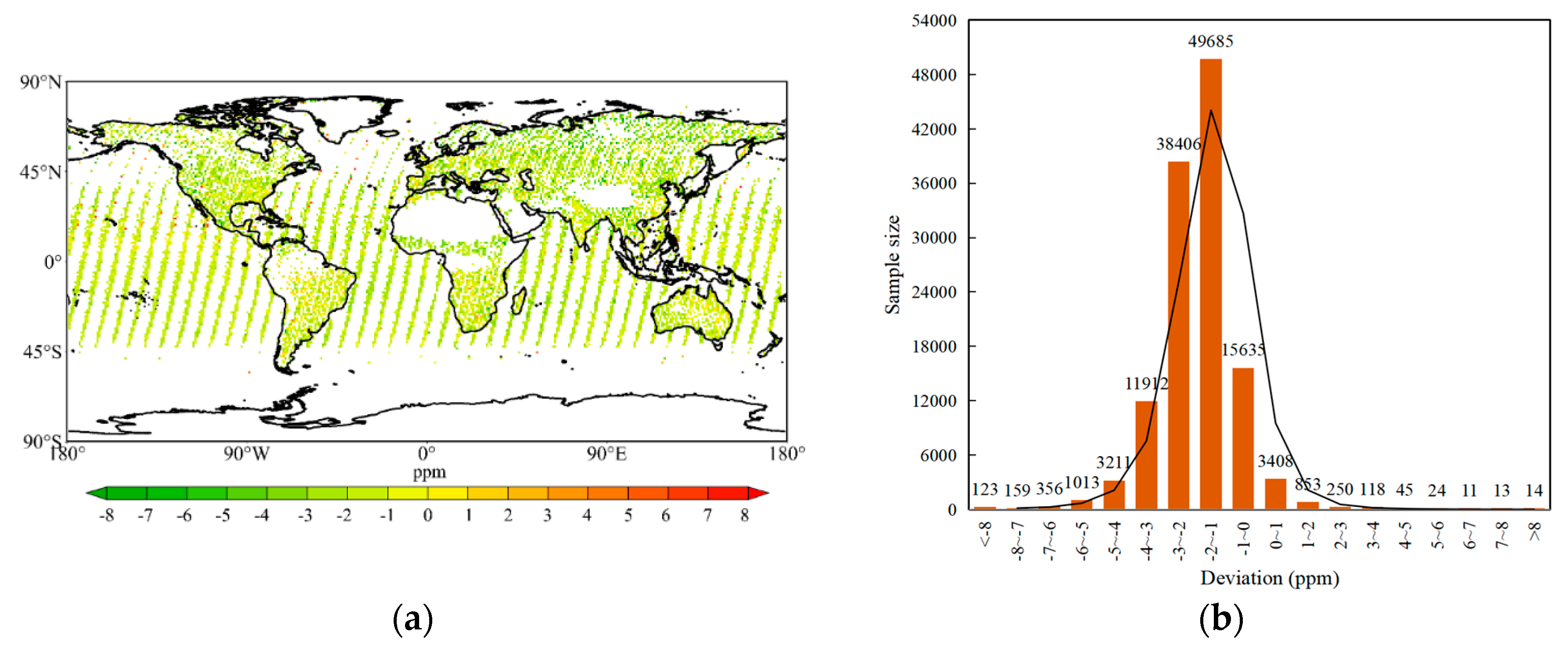
Table 3 presents the total number of samples, mean values of simulated XCO2 and GOSAT XCO2, standard deviation (SD), root mean square error (RMSE), and correlation coefficient (r) for each month, providing a comparison of the simulated and observed XCO2 on a monthly scale. A total of 125,236 observed samples were collected throughout the year. The standard deviations of both simulated and observed XCO2 exhibited similar trends over the course of the year, and the RMSE for both was below 2.48 ppm. The correlation coefficient for most months exceeded 0.62, with an overall annual correlation coefficient reaching 0.79. In general, the simulated XCO2 concentrations were 0 to 2.00 ppm lower than the GOSAT XCO2 concentrations. However, both datasets showed high consistency in terms of spatial and temporal distribution, indicating that the GEOS-Chem simulation results in this study accurately reflect the satellite observation data.
3.1.2. Verification Results of Surface Observation
The simulated surface CO2 concentrations were derived using the method described in Section 2.3.2 and compared with the CO2 concentration data from 30 selected NOAA-ESRL surface observation sites. The correlation coefficients between the simulated and observed surface CO2 concentrations at all sites are shown in Supplementary Information (SI) Figure S1. At more than 90% of the sites, the correlation coefficient exceeded 0.85, and at over half of the sites, it exceeded 0.95. As shown in Figure 2, CO2 concentrations at all stations exhibited a general upward trend over the years and displayed different seasonal variations with respect to latitude. Specifically, the observed surface CO2 concentration in the high latitudes of the Northern Hemisphere, particularly in Europe, showed significant seasonal variation. For example, the annual fluctuation in observed surface CO2 concentrations at sites such as PAL, HUN, BAL, BSC, BRW, ALT, UUN, and MHD reached about 20 ppm. In contrast, surface CO2 concentrations in the Southern Hemisphere exhibited smaller fluctuations throughout the year. For example, at sites like USH, BKT, PSA, SEY, ASC, HBA, SYO, and CGO, the annual fluctuation in surface CO2 concentrations was less than 5 ppm. The simulated surface CO2 concentrations were highly consistent with those observed at about 80% of the sites, with the mean deviation being less than 2.5 ppm. Overall, the surface CO2 concentrations simulated by GEOS-Chem in this study align well with the observations from NOAA-ESRL, indicating that the simulation results accurately reflect the spatial and temporal distribution of CO2 concentrations in the real atmosphere.
3.2. Temporal and Spatial Characteristics of Global Simulated Atmospheric CO2 Concentration
The annual average surface CO2 concentration simulated by GEOS-Chem from 2006 to 2010, as shown in Figure 3 (a), reveals a global average of 383.7 ppm. The data indicate that CO2 concentrations over land are consistently higher than over the oceans, and concentrations in the Northern Hemisphere exceed those in the Southern Hemisphere. Specifically, CO2 concentrations in most of the Northern Hemisphere are above 384 ppm, while in the Southern Hemisphere, particularly south of 20°S, CO2 concentrations generally remain below 382 ppm. These regional variations are primarily influenced by natural factors such as the ocean and terrestrial biosphere, which act as carbon sinks, absorbing some of the CO2 and thereby lowering atmospheric concentrations. Our study finds that CO2 concentrations are particularly high in industrialized and densely populated regions such as eastern China, Southeast Asia, northern Eurasia, Europe, and eastern North America, where the average annual CO2 concentration ranges from 394 to 406 ppm. These findings are consistent with those reported by Miller et al. (2019) [37] and Hamble et al. (2021) [38], who observed that industrialization and high energy consumption lead to elevated CO2 levels in these areas. Miller et al. (2019) [37] highlighted the role of energy consumption and air pollution in driving high CO2 concentrations in industrialized regions, a trend that aligns with our own results.
In contrast, CO2 concentrations in the Southern Hemisphere are generally lower; however, elevated CO2 levels are observed in northern South America and Central Africa. Specifically, in northern South America, the average annual CO2 concentration exceeds 398 ppm, and in parts of Central Africa, concentrations can reach over 396 ppm. These findings are in line with Xie et al. (2024) [39], who demonstrated that deforestation, natural gas extraction, and fossil fuel activities are significant contributors to the rise in CO2 concentrations in these regions. Therefore, while there are notable regional differences in global CO2 concentrations, these variations are not only driven by natural factors but also by anthropogenic activities such as industrialization, deforestation, and fossil fuel extraction, which is consistent with findings from various studies.
As shown in Figure 3 (b), the average annual growth rate of surface CO2 concentration simulated by GEOS-Chem from 2006 to 2010 is 1.8 ppm year⁻¹. There are significant regional variations in the CO2 growth rates. Eastern China exhibits the fastest annual increase in CO2 concentration, with the maximum rate reaching up to 3.0 ppm year⁻¹. This rapid growth is primarily driven by the high population density and intense industrial energy consumption in Eastern China, where industrial emissions are the principal contributor to the accelerated rise in atmospheric CO2 levels. These findings align with the study by Liu et al. (2024) [40], which underscores the substantial emissions from industrial activities, particularly in densely populated urbanized regions of eastern China. In addition to Eastern China, regions such as Southeastern North America, northern South America, Europe, and Central Africa show annual CO2 growth rates ranging from 1.8 to 2.4 ppm year⁻¹. These regions also experience elevated industrial emissions, further corroborating the observed higher CO2 growth rates. However, Southeast Asia stands out with a significantly lower growth rate, averaging around 1.5 ppm year⁻¹, compared to other high-emission regions. This disparity can be attributed to lower industrial emissions and less intensive energy consumption in Southeast Asia. Research by Liu et al. (2023) [41] suggests that despite rapid industrialization, Southeast Asia still exhibits lower per capita CO2 emissions compared to regions such as China and North America, leading to a relatively lower growth rate in atmospheric CO2 concentration.
The global distribution of CO2 concentrations exhibits typical seasonal variation characteristics (Figure 4). Winter is the season with the highest CO2 concentration of the year, with a global average simulated CO2 concentration of 385.4 ppm. In regions such as much of Europe, northern Eurasia, and southeastern China, CO2 concentrations exceed 400 ppm, and in parts of central Europe, central Asia, and eastern China, concentrations even surpass 410 ppm. Summer, on the other hand, is the season with the lowest CO2 concentration, with a global average simulated CO2 concentration of 381.5 ppm. During this period, CO2 concentrations are highest near the equator, ranging from 380 to 400 ppm. North of 45°N, CO2 concentrations are generally below 380 ppm, and in some areas of central Europe, concentrations can even drop below 370 ppm. The CO2 concentration in spring and autumn lies between that of winter and summer, with the high-concentration regions showing a distribution similar to that of winter. These seasonal variations can be attributed to changes in temperature and biological activity. In winter, due to lower temperatures and increased heating demands, as well as higher energy consumption in industrialized regions, CO2 concentrations rise, especially in regions such as eastern China and Europe. In contrast, during the summer, increased photosynthesis by plants leads to significant CO2 absorption, resulting in lower concentrations, particularly in the higher latitudes of the Northern Hemisphere where vegetation growth and temperature conditions have a suppressive effect on CO2 levels [42]. Moreover, the CO2 concentrations in spring and autumn are intermediate, influenced by the combined effects of temperature, plant activity, and climatic conditions [43]. Therefore, seasonal fluctuations are not only a natural consequence of climate changes but also the result of the interplay between biological and human activities, especially in industrialized and energy-intensive areas where CO2 concentrations fluctuate more significantly.
Figure S2 shows the global average surface CO2 concentration for each month from 2006 to 2010 as simulated by GEOS-Chem. The global average CO2 concentration has increased rapidly year by year, and the atmospheric CO2 concentration has increased by about 7.0 ppm in 5 years. The regression line was obtained by linear fitting of monthly CO2 concentration, and it can be inferred that the CO2 concentration increased by about 0.13 ppm per month, and the coefficient of determination reached more than 0.42. In addition, it can be seen from the figure that the global atmospheric average CO2 concentration has significant seasonal fluctuations.
Figure S3 shows the monthly average global surface CO2 concentration and growth rate, which is used to further explore the month-to-month variation of global CO2 concentration. As can be seen from the figure, the global average CO2 concentration has an obvious seasonal fluctuation cycle, and the global average CO2 concentration gradually increases from January to March, reaching the annual peak value (389.3 ppm), and then gradually decreases, reaching the annual trough value (383.1 ppm) in August, and the difference of CO2 concentration in each month of the year is up to 6.2 ppm. In contrast, the month-to-month trend of the growth rate of global mean CO2 concentration shows an inverse phase change compared with CO2 concentration. The growth rate of CO2 concentration in September was the highest (1.95 ppm year-1), and the growth rate of CO2 concentration in February was the lowest (1.62 ppm year-1), and the difference of monthly CO2 concentration growth rate throughout the year was the highest at 0.33 ppm year-1.
3.3. Effects of Different CO2 Sources on Atmospheric CO2 Concentration
Figure 5 and Table S2 shows the global fluxes of eight different types of CO2 source sinks simulated by GEOS-Chem in this study. Among them, fossil fuel emissions mainly include CO2 emissions from natural gas, coal, oil and other fossil fuels. Biomass combustion emissions are mainly CO2 emissions from forest fires, grassland fires, crop straw burning, household firewood burning, domestic waste burning and so on. Equilibrium biosphere refers to the net ecosystem productivity calculated by the sum of total primary productivity and respiration without considering anthropogenic influence, with seasonal cyclical changes, but the annual net total is 0. Nautical emissions are the emissions caused by Marine navigation activities. Aviation emissions include CO2 emissions from aviation activities at every layer of the atmosphere. Ocean exchange refers to the amount of CO2 exchanged between the ocean and the atmosphere. Chemical sources mainly include the oxidation of carbon monoxide, methane and other species into CO2 in the atmosphere. According to the simulation results, fossil fuel combustion is the world’s largest source of CO2 emissions, emitting 8.81 Gt C year-1 into the atmosphere. Biomass combustion is the second largest source of CO2 emissions globally, emitting 2.00 Gt C year-1 into the atmosphere, accounting for about a quarter of fossil fuel emissions. Aviation and navigation emit less than 0.3 Gt C of CO2 into the atmosphere throughout the year, but as an important source of CO2 in the atmosphere, their role cannot be ignored. The land and ocean are the most important CO2 sinks in the world and maintain the dynamic balance of CO2 in the atmosphere by absorbing CO2. The land and ocean are the most important CO2 sinks in the world, and maintain the dynamic balance of CO2 in the atmosphere by absorbing CO2.
In the process of industrialization and urbanization, global CO2 emissions from fossil fuels have been increasing over the past few decades. The regional distribution of fossil fuel emissions is uneven, with the largest emitters globally being China, the United States and India, but some small countries and regions have high per capita emissions. In addition, there are differences in the energy structure of fossil fuels, such as some countries’ energy mainly comes from fossil fuels such as coal, while others rely on natural gas, nuclear energy and other energy sources. The burning of fossil fuels releases large amounts of CO2, far more than other sources of emissions. Global CO2 emissions from fossil fuels are one of the main causes of climate change, and the CO2 produced can persist in the atmosphere for decades or even longer, causing global warming and climate crisis, and becoming a global problem [44].
As can be seen from the global distribution of fossil fuel emissions in Figure 6 (a), the high value area of fossil fuel emissions is mainly distributed in the northern Hemisphere, especially in the United States, Europe, India, China and other regions, and the local annual CO2 emissions can even exceed 2500 g C/m2. There are also pockets of high fossil fuel emissions along the southeastern coast of South America, Africa and Australia. The spatial distribution of fossil fuel emissions depends on many factors, including geographic location, level of economic development, energy use patterns, industrial structure, population density, and more. Some developed countries and developing countries have a large number of factories and energy consumption facilities, such as power plants and gas stations, national economic development level is high, rapid development, accompanied by high energy consumption. The spatial distribution characteristics of surface atmospheric CO2 concentration affected by fossil fuel emissions (Figure 6 (b)) are very similar to the spatial distribution characteristics of fossil fuel emissions themselves. The increase in CO2 concentration caused by fossil fuel emissions is more pronounced in the Northern Hemisphere than in the Southern Hemisphere, which is in contrast to the more intensive population, economic and industrial development in the Northern Hemisphere. Increases in CO2 concentrations are particularly significant in eastern North America, Europe and eastern Asia. The added value of CO2 concentration caused by fossil fuel emissions generally exceeds 5 ppm in eastern North America, reaching a maximum of 13 ppm, generally exceeds 7 ppm in Europe, reaching a maximum of about 15 ppm, and generally exceeds 8 ppm in eastern China, reaching a maximum of about 25 ppm.
In The Global Carbon Budget 2023 report states that land use change carbon emissions are the second largest source of CO2 emissions after fossil fuel combustion, of which biomass combustion is an important component. In some developing countries and regions, biomass combustion dominates all sources of carbon emissions [45]. Unlike fossil fuel emissions, CO2 emitted from biomass combustion is not a new carbon source, but comes from atmospheric CO2 previously absorbed by plants, so biomass energy is also considered a renewable energy source [46]. Biomass combustion has strong spatial and temporal heterogeneity, showing randomness, periodicity, wide range, multi-point sources, difficult monitoring and other characteristics, and has a very important contribution to the spatial and temporal distribution and dynamic changes of global CO2. Biomass burning will have an impact on the climate in the short term, but the impact on the climate in the long term is dynamically balanced. However, the problems brought by land use change, water resource consumption, and deforestation still need people’s attention.
As can be seen from Figure 7 (a), carbon emissions from biomass combustion are widely distributed globally, particularly in key regions such as Africa, South America, and the Southeast Asian Peninsula, where it significantly impacts atmospheric CO2 concentrations. In Africa, biomass burning activities are primarily concentrated in central and southern regions, with annual CO2 emissions generally exceeding 15 g C/m², and in some areas, surpassing 400 g C/m². This results in an increase in near-surface atmospheric CO2 concentrations of more than 4.0 ppm throughout the year. These findings identified that biomass burning in Africa and the Amazon Basin leads to similar annual CO2 concentration increases of up to 4 ppm.
Moreover, this study finds that biomass combustion in central and eastern South America and the Southeast Asian Peninsula also significantly influences local atmospheric CO2 levels (Figure 7 (b)), with annual CO2 emissions typically above 25 g C/m², resulting in CO2 concentration increases exceeding 1.2 ppm. This is consistent with the findings of [47]who reported that biomass burning in Southeast Asia, particularly in Indonesia, can lead to CO2 concentration increases ranging from 1.5 to 2.0 ppm. Similarly, Andreae and Merlet (2001) [48]provided comparable data, indicating that during fire seasons, CO2 concentration increases in Africa and South America could reach 3–4 ppm, further validating the observations made in this study.
By comparing these results with existing research, it is evident that the data from this study are in strong agreement with previous findings, reinforcing the significant impact of biomass combustion on global CO2 concentrations, especially in critical regions like Africa, South America, and Southeast Asia. These findings are crucial for understanding the global carbon cycle and its implications for climate change.
Influenced by climate change, soil moisture, vegetation growth, soil temperature and land use patterns, CO2 flux between vegetation and ecosystem has obvious seasonal fluctuations [49]. The equilibrium biosphere exchange flux in the GEOS-Chem model refers to the net difference between the total amount of CO2 absorbed by plants through photosynthesis and the total amount of ecosystem respiration, which has seasonal characteristics, but the total annual flux remains 0. Specifically, summer is usually the strongest season for CO2 absorption, because vegetation growth and photosynthesis are enhanced in summer, which increases the absorption of CO2 from the atmosphere. The strongest release of CO2 from plants occurs in winter, when vegetation growth slows and soil respiration increases, leading to an increase in CO2 release into the atmosphere. Based on this feature, this study analyzed the equilibrium biosphere exchange flux and its impact on atmospheric CO2 concentration on a seasonal scale.
Figure 8 (a)-(d) shows the equilibrium biosphere exchange carbon flux for the four seasons. Positive values generally represent net CO2 fluxes from ecosystems to the atmosphere (known as terrestrial carbon sources), and negative values represent net CO2 removals from the atmosphere to ecosystems (known as terrestrial carbon sinks). Areas where equilibrium biosphere exchange fluxes are prominent coincide highly with areas with dense vegetation, with significant seasonal variations. In winter, the equilibrium biosphere exchange flux is dominated by terrestrial carbon sources in the equatorial regions of South America and Africa, North America, Eurasia except India, and Australia, and peaks in Europe at more than 600 g C/m2. South of the equator, South America, Africa and India are dominated by terrestrial carbon sinks, and the overall carbon sinks are weak. In summer, terrestrial carbon sinks dominate equatorial regions and the northern hemisphere. The northern Central Asia region has the strongest carbon sink, with local carbon sinks exceeding 900 g C/m2. The carbon sink in the northern part of North America is also very prominent, generally distributed above 500 g C/m2. The equilibrium biosphere exchange fluxes in spring and autumn are significantly lower in order of magnitude than in winter and summer, and the distribution of terrestrial carbon sources and carbon pools are also different. It is worth noting that the terrestrial carbon source effect in India is the strongest in the spring, and the whole region is basically more than 300 g C/m2. The changes of surface atmospheric CO2 concentration caused by the equilibrium biosphere exchange flux (Figure 8 (e)-(h)) also have seasonal fluctuations. The equilibrium biosphere exchange flux causes a significant increase in atmospheric CO2 concentration in winter, which is evident in northern and eastern North America, equatorial South America, Africa and Indonesia, northern Eurasia, southeast Asian peninsula and central and eastern China. The increase of CO2 concentration in Eurasia is generally more than 9 ppm. In summer, the balanced biosphere flux resulted in a general reduction of CO2 concentrations of more than 7 ppm in continental regions north of 45° N latitude. It is worth noting that the equatorial regions of South America, Africa and Indonesia show an increasing trend of CO2 caused by the equilibrium biosphere exchange flux throughout the year, which plays a key role in the change of atmospheric CO2 concentration due to the vigorous growth of vegetation in tropical regions, such as tropical rainforests and savannas.
The net land exchange flux is used to represent the net annual budget or residual amount of CO2 from the terrestrial biosphere. In the GEOS-Chem model, this partial CO2 flux is set to a fixed value and divided according to different regions. A total of 11 subregions have been identified on a global scale, and the net land exchange flux within each subregion is nearly consistent. According to Figure 9 (a), Northern North America and South America are the two most typical net terrestrial exchange carbon sources in the world, while other regions are net terrestrial exchange carbon sinks, the top three regions are Southern Africa, Europe and Southern South America. The global net land exchange flux was -5.28 Gt C, dominated by carbon sinks throughout the year. Correspondingly, the surface atmospheric CO2 concentration affected by the net land exchange flux (Figure 9 (b)) showed similar distribution characteristics, and the overall performance of the whole year was to reduce the atmospheric CO2 concentration. In northern South America, the change in atmospheric CO2 concentration due to net land exchange flux was less than 0.8 ppm, and in Europe, the change in atmospheric CO2 concentration due to net land exchange flux was more than 4.4 ppm.
Navigation is one of the important sources of greenhouse gas emissions from human activities. According to the third study of greenhouse gas emissions published by the International Maritime Organization (IMO), CO2 emissions from shipping account for about 2.2% of the total global CO2 emissions. In 2018, the total CO2 emissions of the global shipping industry were 1.01 billion tons, of which the CO2 emissions of maritime transport were 960 million tons, accounting for more than 95%, occupying a dominant position in shipping. CO2 emissions from land transport and port activities are smaller, at 0.4 million tonnes and 0.1 million tonnes respectively. In addition, CO2 emissions from the shipping industry continue to grow, with global CO2 emissions from shipping increasing by 28.9% between 2007 and 2018, with the number of ships increasing by more than 50%. At the same time, the improvement of ship transportation efficiency and fuel utilization rate can only partially offset the increase in emissions caused by the increase in the number of ships [50,51].
Figure 10 (a) shows the spatial distribution of global maritime carbon emissions in 2010. The high value areas of Marine carbon emissions are closely consistent with Marine activities, and the coastal areas and common routes are usually the areas with high CO2 emissions. This is because these areas usually have a large number of ports and transportation, which requires a large amount of fuel consumption. Maritime CO2 emissions from European coastal areas are among the highest in the world, exceeding 500 g C/m2 in some areas. This is because the European region has many ports and shipping centers, its maritime transport business is large, and the corresponding carbon emissions are relatively high. Secondly, the economic activity of Europe’s coastal regions is intensive, including several industries such as manufacturing, trade and tourism, which require a large amount of support from shipping services, further increasing shipping carbon emissions. In addition, the European coastal region has a large maritime fleet, and these vessels often use traditional oil power systems and have relatively high carbon emissions. The spatial distribution of global atmospheric CO2 concentration increase caused by navigation (Figure 10 (b)) is highly consistent with Marine CO2 emissions, in which the increase of CO2 concentration in the northern Hemisphere is significantly higher than that in the Southern Hemisphere, and it is mainly distributed in the two sides of the Atlantic and Pacific oceans. Coastal areas in northern Germany and Denmark have the highest CO2 increases in the world, with local CO2 increases from Marine CO2 emissions reaching up to 0.48 ppm or more.
Aviation activities are a significant source of global greenhouse gas emissions. The bulk of aviation’s carbon emissions come from CO2 produced by burning fuel in jet engines. According to the International Civil Aviation Organization (ICAO), CO2 emissions from aviation account for about 2–3% of total global CO2 emissions. Carbon emissions from aviation have grown over the past few decades and are expected to continue to increase in the future. The International Energy Agency (IEA), based on future economic growth and expansion of the aviation industry, as well as technology and policy measures for the aviation industry in the future, predicts that global carbon emissions from the aviation industry could grow 2–3 times by 2040. IEA 2023 report, “The Future of Petrochemicals: Towards more sustainable plastics and fertilisers” Long-haul international flights have relatively high carbon emissions because they use more fuel. Short-haul flights have relatively low carbon emissions. In addition, the impact of CO2 emitted at high altitude on climate change is more significant than that of CO2 emitted at ground level. This is because, in addition to ground airports, aviation carbon emissions mainly occur at high altitude, high-altitude CO2 emissions can be more easily dispersed around the world, and its greenhouse effect is more intense at high altitude. For example, the Fifth Assessment report released by the United Nations Intergovernmental Panel on Climate Change (IPCC) pointed out that the contribution of carbon emissions from aviation activities to global warming is about 3.5–4.9%.
Affected by many factors such as flight route, flight speed, aircraft type and meteorological conditions, the height of aviation carbon emissions is not fixed. Figure 11 (a) shows the aggregate CO2 emissions from aviation at each vertical level of the atmosphere. Aviation CO2 emissions are highly consistent with airport locations, showing the locations of major global air terminals. Among them, the United States, Europe, southeast China and Japan are the regions with the highest emissions of global aviation, with emissions reaching more than 20 g C/m2. In addition, the distribution of aviation emissions is closely related to the route, and this part comes from the CO2 emitted by the aircraft during flight. Unlike other sources of emissions, aviation CO2 emissions occur at both surface and high altitudes, and at different altitudes in different parts of the world. Therefore, this study explores the impact of aviation emissions on the average atmospheric CO2 concentration at each layer. As can be seen from Figure 11 (b), the increase in the mean atmospheric CO2 concentration of each layer caused by aviation CO2 emissions is higher in the northern Hemisphere and lower in the Southern Hemisphere. Due to the enhanced mixing in the upper atmosphere, the distribution of CO2 concentration is zonally uniform across the globe, with a north-south gradient of about 0.04 ppm. At the same time, this study also explored the changes in surface atmospheric CO2 concentration affected by aviation CO2 emissions in 2010 (Figure S4). The increase of surface CO2 concentration was also high in the northern Hemisphere and low in the Southern Hemisphere, but it was prominent in the continental region. Among them, the United States and Europe are the two major regions where the surface atmospheric CO2 concentration increased significantly due to aviation CO2 emissions, and the local CO2 concentration increase value can reach more than 0.1 ppm, and it is one-to-one corresponding to the airport location.
CO2 exchange between the ocean and atmosphere is one of the important processes affecting the global carbon cycle and one of the important factors affecting global climate change. Overall, the ocean, as a major global carbon sink, absorbs about 25% of CO2 emissions from the atmosphere, which plays an important role in regulating climate and mitigating the greenhouse effect [52]. In tropical areas, the temperature of the sea surface is higher, and these areas usually have a greater amount of sunlight. As a result, the oceans in these areas typically release CO2; In polar sea regions, sea surface temperatures are cooler, and the amount of sunlight in these regions is generally less. As a result, the oceans in these regions typically absorb CO2 [53]. The rate at which the ocean absorbs CO2 from the atmosphere varies with the seasons, with a faster rate in winter and a slower rate in summer. The surface of the ocean is the main area of CO2 absorption and release, and the deep ocean usually has relatively high CO2 concentrations. Ocean circulation also has an important effect on the exchange of CO2 between the ocean and the atmosphere. For example, ocean circulation around Antarctica typically results in the release of large amounts of CO2 from the region’s oceans [54].
Figure 12 (a) shows the global ocean exchange carbon flux, representing the exchange of CO2 between the ocean and the atmosphere. Positive values indicate that CO2 enters the atmosphere from the ocean, that is, the ocean emits CO2 (Marine CO2 source); Negative values represent the passage of CO2 from the atmosphere into the ocean, i.e. the uptake of CO2 by the ocean (ocean CO2 sink). As can be seen from the figure 12 (a), the tropical region and the circumantarctic region are the main sources of ocean CO2 exchange in the world, among which the tropical eastern Pacific region and the junction of the Arabian Sea and the Gulf of Aden are the regions with the strongest annual Marine CO2 emission, with a local maximum of more than 36 g C/m2. The Norwegian Sea and Labrador Bay near the Arctic Circle are the two regions with the strongest annual Marine CO2 absorption, with local CO2 absorption fluxes reaching above 54 g C/m2. As can be seen from Figure 12 (b), the impact of ocean exchange on surface atmospheric CO2 concentration is mainly manifested as the reduction of global CO2 concentration. Specifically, changes in CO2 concentrations at the ocean surface decrease from the equator to the poles. The annual ocean exchange flux decreased the CO2 concentration in the equatorial waters by 0~0.8 ppm. The CO2 concentration in the sea area near 45° S latitude decreased by 1.1~1.5 ppm; The CO2 concentration in the North Atlantic Ocean to the south of the Arctic Ocean decreased by more than 1.2 ppm, of which the highest CO2 concentration in the east and south of Greenland exceeded 1.6 ppm.
The CO2 emission inventory in the traditional atmospheric model ignores the CO2 produced by oxidation of other carbon species. This simulation process has defects and lacks comprehensive consideration of the CO2 generation process, which will lead to inaccurate simulation results. In order to more accurately simulate global atmospheric CO2 levels, Nassar et al (2010) [55] improved the CO2 emission inventory of the GEOS-Chem model to take into account CO2 produced by oxidation of other carbon species, such as biomass burning, land use change, and forest harvesting. In addition, there are other carbon species that may produce CO2, such as weathering of carbonate rocks and respiration of aquatic organisms. These oxidation effects can lead to the release of CO2 into the atmosphere, which has an impact on global climate change. Taking into account the chemical source flux of CO2 produced by the oxidation of carbon species, the model can more accurately simulate global atmospheric CO2 levels and provide more accurate data to guide the development and implementation of global climate change policies.
As can be seen from Figure 13 (a), the CO2 generated by oxidation of other species is subtracted in the simulation, that is, the model simulation results are corrected. The flux of chemical sources is widely distributed globally, which is the result of the comprehensive action of multiple processes and species oxidation of CO2 in the region. Eastern North America, South America, Europe, Central Africa, South Asia, and Southeast Asia are several regions with large chemical source fluxes Figure 13 (b), which are basically above 10 g C/m2. The variation of surface CO2 concentration affected by chemical source flux is very consistent with the distribution of chemical source flux, which is mainly manifested by reducing and correcting the simulated CO2 concentration. Chemical source fluxes widely cause CO2 concentration changes on a global scale, among which, central Africa and eastern China are the regions most affected by chemical source fluxes, and the maximum annual CO2 concentration change can exceed 1.0 ppm, which is closely related to a large number of biomass burning. In addition, in eastern North America, South America, northern Africa, Europe, Asia and Southeast Asia, the CO2 concentration change value is basically above 0.25 ppm.
4. Conclusions
The study shows that fossil fuel combustion is the largest source of atmospheric CO2 emissions, reaching 8.81 Gt C/year, and biomass combustion is the second largest source of CO2 emissions, reaching about a quarter of fossil fuel combustion in 2010, reaching 2.00 Gt C/year. In addition, aviation emissions, Marine emissions, chemical reactions also have a greater contribution to atmospheric CO2 emissions. The ocean is a very important sink of atmospheric CO2, absorbing 2.22 Gt C/year from the atmosphere, and the terrestrial biosphere is also an important sink of atmospheric CO2, with a net terrestrial ecosystem exchange of 5.28 Gt C/year.
The influence of different CO2 source flux on atmospheric CO2 concentration is highly correlated with the spatial distribution and flux magnitude of CO2 source flux, and is highly consistent in spatial distribution. Specifically: Emissions from fossil fuel combustion are significantly greater in the Northern Hemisphere than in the southern Hemisphere, with particularly large emissions in the eastern United States, Europe, East Asia, and India. Global emissions from fossil fuel combustion have caused the increase in atmospheric CO2 concentration, and fossil fuel combustion in the northern hemisphere has a greater impact on atmospheric CO2, and the largest contribution is in eastern China. CO2 emissions from biomass combustion are widely distributed in the world, and Africa is the land region that contributes the most to global biomass combustion emissions. The spatial distribution of CO2 concentration increase caused by biomass combustion emission is similar to that of biomass combustion emission itself. Among them, South America, Africa and Southeast Asian peninsula are the three regions most affected by biomass combustion emissions, and the increase of CO2 concentration is particularly obvious. The seasonal variation of atmospheric CO2 source and sink caused by the equilibrium biosphere also resulted in the corresponding seasonal variation of atmospheric CO2 concentration. In summer, the equilibrium biosphere reduces the atmospheric CO2 concentration in the northern Hemisphere and increases the atmospheric CO2 concentration in some parts of the Southern hemisphere. North America and the northern part of South America are two typical net terrestrial exchange carbon sources in the world, while the other regions are net terrestrial exchange carbon sinks. The net terrestrial exchange flux has corresponding effects on atmospheric CO2 concentration, and the spatial distribution characteristics correspond to the net terrestrial exchange flux. Aviation and maritime activities are important sources of global atmospheric CO2 emissions. Aviation emissions and maritime emissions are mainly concentrated on their respective routes, as well as airports for aircraft and ports for ships. The spatial distribution of global atmospheric CO2 concentration increase caused by aviation emissions and maritime emissions corresponds to the spatial distribution of CO2 emissions themselves. The ocean is primarily a sink for atmospheric CO2. The tropical region and the circumantarctic region are the main global sources of ocean CO2 exchange, and the Norwegian Sea and Labrador Bay near the Arctic Circle are the two regions with the strongest ocean CO2 absorption throughout the year. The impact of ocean exchange on surface atmospheric CO2 concentration is mainly manifested in the reduction of global CO2 concentration. Atmospheric CO2 chemical reaction sources are widely distributed around the world and are mainly used to quantify the oxidation of carbon species to produce CO2. The effect of chemical sources on atmospheric CO2 concentration is mainly used to reduce the simulated CO2 concentration in the model. China and Central Africa are the regions with the strongest chemical reaction sources.
Supplementary Materials
This supplementary document contains Figure S1-Figure S4, Table S1-Table S2.
Author Contributions
Conceptualization, G.Q. and Y.S.; Data curation, Y.Y. and M.S.; Formal analysis, M.S.; Funding acquisition, J.Z.; Investigation, G.Q., W.W. and Z.Z.; Methodology, Y.S.; Project administration, J.Z. and Y.S.; Resources, M.S.; Software, Y.Y.; Supervision, Y.S.; Validation, W.W. and Z.Z.; Visualization, Y.Y.; Writing – original draft, G.Q.; Writing – review & editing, G.Q. and Y.Y. All authors have read and agreed to the published version of the manuscript.
Funding
This research is supported by the National Key Research and Development Program of China (2023YFB3907404), the FY-3 Lot 03 Meteorological Satellite Engineering Ground Application System Ecological Monitoring and Assessment Application Project Phase I (ZQC-R22227), the National Natural Science Foundation of China (42071398), the Heilongjiang Provincial Natural Science Foundation (PL2024D013) and the Academic Innovation Project of Harbin Normal University (HSDBSCX2021-104).
Data Availability Statement
Data of the results of this study can be obtained upon request.
Acknowledgments
We would like to express our sincere gratitude to Researcher Yu-Sheng Shi and Professor Jia Zhou for their invaluable guidance in shaping the framework of this paper. Special thanks to Yongliang Liang and Mengqian Su for their diligent work on data analysis and detail modifications. We also appreciate the support from the Institute of Space and Astronautical Information Innovation, Chinese Academy of Sciences, in building the information platform.
Conflicts of Interest
The authors declare no conflicts of interest.
References
- Friedlingstein, P.; O’Sullivan, M.; Jones, M.W.; Andrew, R.M.; Hauck, J.; Landschützer, P.; Le Quéré, C.; Li, H.; Luijkx, I.T.; Olsen, A.; et al. Global Carbon Budget 2024 2024.
- Bauska, T.K.; Joos, F.; Mix, A.C.; Roth, R.; Ahn, J.; Brook, E.J. Links between Atmospheric Carbon Dioxide, the Land Carbon Reservoir and Climate over the Past Millennium. Nat Geosci 2015, 8, 383–387. [Google Scholar] [CrossRef]
- Keenan, T.F.; Prentice, I.C.; Canadell, J.G.; Williams, C.A.; Wang, H.; Raupach, M.; Collatz, G.J. Recent Pause in the Growth Rate of Atmospheric CO2 Due to Enhanced Terrestrial Carbon Uptake. Nat Commun 2016, 7, 13428. [Google Scholar] [CrossRef]
- Kukkonen, J.; Olsson, T.; Schultz, D.M.; Baklanov, A.; Klein, T.; Miranda, A.I.; Monteiro, A.; Hirtl, M.; Tarvainen, V.; Boy, M.; et al. A Review of Operational, Regional-Scale, Chemical Weather Forecasting Models in Europe. Atmos Chem Phys 2012, 12, 1–87. [Google Scholar] [CrossRef]
- Feng, L.; Palmer, P.I.; Yang, Y.; Yantosca, R.M.; Kawa, S.R.; Paris, J.-D.; Matsueda, H.; Machida, T. Evaluating a 3-D Transport Model of Atmospheric CO2 Using Ground-Based, Aircraft, and Space-Borne Data. Atmos Chem Phys 2011, 11, 2789–2803. [Google Scholar] [CrossRef]
- Zeng, N.; Han, P.; Liu, Z.; Liu, D.; Oda, T.; Martin, C.; Liu, Z.; Yao, B.; Sun, W.; Wang, P.; et al. Global to Local Impacts on Atmospheric CO2 from the COVID-19 Lockdown, Biosphere and Weather Variabilities. Environmental Research Letters 2022, 17, 015003. [Google Scholar] [CrossRef]
- Suntharalingam, P.; Spivakovsky, C.M.; Logan, J.A.; McElroy, M.B. Estimating the Distribution of Terrestrial CO2 Sources and Sinks from Atmospheric Measurements: Sensitivity to Configuration of the Observation Network. Journal of Geophysical Research: Atmospheres 2003, 108. [Google Scholar] [CrossRef]
- Nassar, R.; Jones, D.B.A.; Suntharalingam, P.; Chen, J.M.; Andres, R.J.; Wecht, K.J.; Yantosca, R.M.; Kulawik, S.S.; Bowman, K.W.; Worden, J.R.; et al. Modeling Global Atmospheric CO2 with Improved Emission Inventories and CO2 Production from the Oxidation of Other Carbon Species. Geosci Model Dev 2010, 3, 689–716. [Google Scholar] [CrossRef]
- Randerson, J.T.; Thompson, M. V.; Conway, T.J.; Fung, I.Y.; Field, C.B. The Contribution of Terrestrial Sources and Sinks to Trends in the Seasonal Cycle of Atmospheric Carbon Dioxide. Global Biogeochem Cycles 1997, 11, 535–560. [Google Scholar] [CrossRef]
- Suntharalingam, P.; Jacob, D.J.; Palmer, P.I.; Logan, J.A.; Yantosca, R.M.; Xiao, Y.; Evans, M.J.; Streets, D.G.; Vay, S.L.; Sachse, G.W. Improved Quantification of Chinese Carbon Fluxes Using CO2 /CO Correlations in Asian Outflow. Journal of Geophysical Research: Atmospheres 2004, 109. [Google Scholar] [CrossRef]
- Nassar, R.; Jones, D.B.A.; Suntharalingam, P.; Chen, J.M.; Andres, R.J.; Wecht, K.J.; Yantosca, R.M.; Kulawik, S.S.; Bowman, K.W.; Worden, J.R.; et al. Modeling Global Atmospheric CO2 with Improved Emission Inventories and CO2 Production from the Oxidation of Other Carbon Species. Geosci Model Dev 2010, 3, 689–716. [Google Scholar] [CrossRef]
- Gelaro, R.; McCarty, W.; Suárez, M.J.; Todling, R.; Molod, A.; Takacs, L.; Randles, C.A.; Darmenov, A.; Bosilovich, M.G.; Reichle, R.; et al. The Modern-Era Retrospective Analysis for Research and Applications, Version 2 (MERRA-2). J Clim 2017, 30, 5419–5454. [Google Scholar] [CrossRef]
- Koster R D, D.A.S. da S.A.M. The Quick Fire Emissions Dataset (QFED): Documentation of Versions 2.1, 2.2 and 2. 2015. [Google Scholar]
- Oda, T.; Maksyutov, S. A Very High-Resolution (1 Km×1 Km) Global Fossil Fuel CO2 Emission Inventory Derived Using a Point Source Database and Satellite Observations of Nighttime Lights. Atmos Chem Phys 2011, 11, 543–556. [Google Scholar] [CrossRef]
- Takahashi, T.; Sutherland, S.C.; Wanninkhof, R.; Sweeney, C.; Feely, R.A.; Chipman, D.W.; Hales, B.; Friederich, G.; Chavez, F.; Sabine, C.; et al. Climatological Mean and Decadal Change in Surface Ocean PCO2, and Net Sea–Air CO2 Flux over the Global Oceans. Deep Sea Research Part II: Topical Studies in Oceanography 2009, 56, 554–577. [Google Scholar] [CrossRef]
- Messerschmidt, J.; Parazoo, N.; Wunch, D.; Deutscher, N.M.; Roehl, C.; Warneke, T.; Wennberg, P.O. Evaluation of Seasonal Atmosphere–Biosphere Exchange Estimations with TCCON Measurements. Atmos Chem Phys 2013, 13, 5103–5115. [Google Scholar] [CrossRef]
- Baker, D.F.; Law, R.M.; Gurney, K.R.; Rayner, P.; Peylin, P.; Denning, A.S.; Bousquet, P.; Bruhwiler, L.; Chen, Y. -H.; Ciais, P.; et al. TransCom 3 Inversion Intercomparison: Impact of Transport Model Errors on the Interannual Variability of Regional CO2 Fluxes, 1988–2003. Global Biogeochem Cycles 2006, 20. [Google Scholar] [CrossRef]
- Hoesly, R.M.; Smith, S.J.; Feng, L.; Klimont, Z.; Janssens-Maenhout, G.; Pitkanen, T.; Seibert, J.J.; Vu, L.; Andres, R.J.; Bolt, R.M.; et al. Historical (1750–2014) Anthropogenic Emissions of Reactive Gases and Aerosols from the Community Emissions Data System (CEDS). Geosci Model Dev 2018, 11, 369–408. [Google Scholar] [CrossRef]
- Olsen, S.C.; Brasseur, G.P.; Wuebbles, D.J.; Barrett, S.R.H.; Dang, H.; Eastham, S.D.; Jacobson, M.Z.; Khodayari, A.; Selkirk, H.; Sokolov, A.; et al. Comparison of Model Estimates of the Effects of Aviation Emissions on Atmospheric Ozone and Methane. Geophys Res Lett 2013, 40, 6004–6009. [Google Scholar] [CrossRef]
- Nassar, R.; Jones, D.B.A.; Suntharalingam, P.; Chen, J.M.; Andres, R.J.; Wecht, K.J.; Yantosca, R.M.; Kulawik, S.S.; Bowman, K.W.; Worden, J.R.; et al. Modeling Global Atmospheric CO2 with Improved Emission Inventories and CO2 Production from the Oxidation of Other Carbon Species. Geosci Model Dev 2010, 3, 689–716. [Google Scholar] [CrossRef]
- Fu, Y.; Liao, H.; Tian, X.; Gao, H.; Jia, B.; Han, R. Impact of Prior Terrestrial Carbon Fluxes on Simulations of Atmospheric CO2 Concentrations. Journal of Geophysical Research: Atmospheres 2021, 126. [Google Scholar] [CrossRef]
- Reddington, C.L.; Conibear, L.; Robinson, S.; Knote, C.; Arnold, S.R.; Spracklen, D. V. Air Pollution From Forest and Vegetation Fires in Southeast Asia Disproportionately Impacts the Poor. Geohealth 2021, 5. [Google Scholar] [CrossRef]
- Gao, M.; Beig, G.; Song, S.; Zhang, H.; Hu, J.; Ying, Q.; Liang, F.; Liu, Y.; Wang, H.; Lu, X.; et al. The Impact of Power Generation Emissions on Ambient PM2.5 Pollution and Human Health in China and India. Environ Int 2018, 121, 250–259. [Google Scholar] [CrossRef]
- Kou, X.; Zhang, M.; Peng, Z.; Wang, Y. Assessment of the Biospheric Contribution to Surface Atmospheric CO2 Concentrations over East Asia with a Regional Chemical Transport Model. Adv Atmos Sci 2015, 32, 287–300. [Google Scholar] [CrossRef]
- Jing, Y.; Wang, T.; Zhang, P.; Chen, L.; Xu, N.; Ma, Y. Global Atmospheric CO2 Concentrations Simulated by GEOS-Chem: Comparison with GOSAT, Carbon Tracker and Ground-Based Measurements. Atmosphere (Basel) 2018, 9, 175. [Google Scholar] [CrossRef]
- Wunch, D.; Toon, G.C.; Blavier, J.-F.L.; Washenfelder, R.A.; Notholt, J.; Connor, B.J.; Griffith, D.W.T.; Sherlock, V.; Wennberg, P.O. The Total Carbon Column Observing Network. Philosophical Transactions of the Royal Society A: Mathematical, Physical and Engineering Sciences 2011, 369, 2087–2112. [Google Scholar] [CrossRef] [PubMed]
- Karbasi, S.; Malakooti, H.; Rahnama, M.; Azadi, M. Study of Mid-Latitude Retrieval XCO2 Greenhouse Gas: Validation of Satellite-Based Shortwave Infrared Spectroscopy with Ground-Based TCCON Observations. Science of The Total Environment 2022, 836, 155513. [Google Scholar] [CrossRef]
- Cogan, A.J.; Boesch, H.; Parker, R.J.; Feng, L.; Palmer, P.I.; Blavier, J. -F. L.; Deutscher, N.M.; Macatangay, R.; Notholt, J.; Roehl, C.; et al. Atmospheric Carbon Dioxide Retrieved from the Greenhouse Gases Observing SATellite (GOSAT): Comparison with Ground-based TCCON Observations and GEOS-Chem Model Calculations. Journal of Geophysical Research: Atmospheres 2012, 117. [Google Scholar] [CrossRef]
- Lindqvist, H.; O’Dell, C.W.; Basu, S.; Boesch, H.; Chevallier, F.; Deutscher, N.; Feng, L.; Fisher, B.; Hase, F.; Inoue, M.; et al. Does GOSAT Capture the True Seasonal Cycle of Carbon Dioxide? Atmos Chem Phys 2015, 15, 13023–13040. [Google Scholar] [CrossRef]
- Morino, I.; Uchino, O.; Inoue, M.; Yoshida, Y.; Yokota, T.; Wennberg, P.O.; Toon, G.C.; Wunch, D.; Roehl, C.M.; Notholt, J.; et al. Preliminary Validation of Column-Averaged Volume Mixing Ratios of Carbon Dioxide and Methane Retrieved from GOSAT Short-Wavelength Infrared Spectra 2010.
- Connor, B.J.; Boesch, H.; Toon, G.; Sen, B.; Miller, C.; Crisp, D. Orbiting Carbon Observatory: Inverse Method and Prospective Error Analysis. Journal of Geophysical Research: Atmospheres 2008, 113. [Google Scholar] [CrossRef]
- Masarie, K.A.; Peters, W.; Jacobson, A.R.; Tans, P.P. ObsPack: A Framework for the Preparation, Delivery, and Attribution of Atmospheric Greenhouse Gas Measurements. Earth Syst Sci Data 2014, 6, 375–384. [Google Scholar] [CrossRef]
- Fu, Y.; Liao, H.; Tian, X.-J.; Gao, H.; Cai, Z.-N.; Han, R. Sensitivity of the Simulated CO2 Concentration to Inter-Annual Variations of Its Sources and Sinks over East Asia. Advances in Climate Change Research 2019, 10, 250–263. [Google Scholar] [CrossRef]
- Li, R.; Zhang, M.; Chen, L.; Kou, X.; Skorokhod, A. CMAQ Simulation of Atmospheric CO2 Concentration in East Asia: Comparison with GOSAT Observations and Ground Measurements. Atmos Environ 2017, 160, 176–185. [Google Scholar] [CrossRef]
- Fu, Y.; Liao, H.; Tian, X.; Gao, H.; Jia, B.; Han, R. Impact of Prior Terrestrial Carbon Fluxes on Simulations of Atmospheric CO2 Concentrations. Journal of Geophysical Research: Atmospheres 2021, 126. [Google Scholar] [CrossRef]
- Chen, Z.H.; Zhu, J.; Zeng, N. Improved Simulation of Regional CO2 Surface Concentrations Using GEOS-Chem and Fluxes from VEGAS. Atmos Chem Phys 2013, 13, 7607–7618. [Google Scholar] [CrossRef]
- Deryugina, T.; Heutel, G.; Miller, N.H.; Molitor, D.; Reif, J. The Mortality and Medical Costs of Air Pollution: Evidence from Changes in Wind Direction. American Economic Review 2019, 109, 4178–4219. [Google Scholar] [CrossRef]
- Deryugina, T.; Heutel, G.; Miller, N.H.; Molitor, D.; Reif, J. The Mortality and Medical Costs of Air Pollution: Evidence from Changes in Wind Direction. American Economic Review 2019, 109, 4178–4219. [Google Scholar] [CrossRef]
- Xie, Y.; He, Y.; Ye, Y.; Liu, C. Employ Mathematical Modeling to Summarize, Analyze, And Predict the Relationship Between Carbon Dioxide and Temperature, Location, And Other Factors. Academic Journal of Science and Technology 2024, 11, 13–20. [Google Scholar] [CrossRef]
- Liu, H.; Zhang, Z.; Cai, X.; Wang, D.; Liu, M. Investigating the Driving Factors of Carbon Emissions in China’s Transportation Industry from a Structural Adjustment Perspective. Atmos Pollut Res 2024, 15, 102224. [Google Scholar] [CrossRef]
- Liu, B.; Guan, Y.; Shan, Y.; Cui, C.; Hubacek, K. Emission Growth and Drivers in Mainland Southeast Asian Countries. J Environ Manage 2023, 329, 117034. [Google Scholar] [CrossRef]
- Forkel, M.; Carvalhais, N.; Rödenbeck, C.; Keeling, R.; Heimann, M.; Thonicke, K.; Zaehle, S.; Reichstein, M. Enhanced Seasonal CO2 Exchange Caused by Amplified Plant Productivity in Northern Ecosystems. Science (1979) 2016, 351, 696–699. [Google Scholar] [CrossRef]
- Lin, X.; Rogers, B.M.; Sweeney, C.; Chevallier, F.; Arshinov, M.; Dlugokencky, E.; Machida, T.; Sasakawa, M.; Tans, P.; Keppel-Aleks, G. Siberian and Temperate Ecosystems Shape Northern Hemisphere Atmospheric CO2 Seasonal Amplification. Proceedings of the National Academy of Sciences 2020, 117, 21079–21087. [Google Scholar] [CrossRef]
- Le Quéré, C.; Jackson, R.B.; Jones, M.W.; Smith, A.J.P.; Abernethy, S.; Andrew, R.M.; De-Gol, A.J.; Willis, D.R.; Shan, Y.; Canadell, J.G.; et al. Temporary Reduction in Daily Global CO2 Emissions during the COVID-19 Forced Confinement. Nat Clim Chang 2020, 10, 647–653. [Google Scholar] [CrossRef]
- Chen, J.; Li, C.; Ristovski, Z.; Milic, A.; Gu, Y.; Islam, M.S.; Wang, S.; Hao, J.; Zhang, H.; He, C.; et al. A Review of Biomass Burning: Emissions and Impacts on Air Quality, Health and Climate in China. Science of The Total Environment 2017, 579, 1000–1034. [Google Scholar] [CrossRef] [PubMed]
- Ji, X.; Long, X. A Review of the Ecological and Socioeconomic Effects of Biofuel and Energy Policy Recommendations. Renewable and Sustainable Energy Reviews 2016, 61, 41–52. [Google Scholar] [CrossRef]
- Field, R.D.; van der Werf, G.R.; Shen, S.S.P. Human Amplification of Drought-Induced Biomass Burning in Indonesia since 1960. Nat Geosci 2009, 2, 185–188. [Google Scholar] [CrossRef]
- Andreae, M.O.; Merlet, P. Emission of Trace Gases and Aerosols from Biomass Burning. Global Biogeochem Cycles 2001, 15, 955–966. [Google Scholar] [CrossRef]
- Philip, S.; Johnson, M.S.; Potter, C.; Genovesse, V.; Baker, D.F.; Haynes, K.D.; Henze, D.K.; Liu, J.; Poulter, B. Prior Biosphere Model Impact on Global Terrestrial CO2 Fluxes Estimated from OCO-2 Retrievals. Atmos Chem Phys 2019, 19, 13267–13287. [Google Scholar] [CrossRef]
- Lee, D.S.; Fahey, D.W.; Skowron, A.; Allen, M.R.; Burkhardt, U.; Chen, Q.; Doherty, S.J.; Freeman, S.; Forster, P.M.; Fuglestvedt, J.; et al. The Contribution of Global Aviation to Anthropogenic Climate Forcing for 2000 to 2018. Atmos Environ 2021, 244, 117834. [Google Scholar] [CrossRef]
- Corbett, J.J.; Winebrake, J.J.; Green, E.H.; Kasibhatla, P.; Eyring, V.; Lauer, A. Mortality from Ship Emissions: A Global Assessment. Environ Sci Technol 2007, 41, 8512–8518. [Google Scholar] [CrossRef]
- Landschützer, P.; Gruber, N.; Bakker, D.C.E.; Schuster, U. Recent Variability of the Global Ocean Carbon Sink. Global Biogeochem Cycles 2014, 28, 927–949. [Google Scholar] [CrossRef]
- Takahashi, T.; Sutherland, S.C.; Wanninkhof, R.; Sweeney, C.; Feely, R.A.; Chipman, D.W.; Hales, B.; Friederich, G.; Chavez, F.; Sabine, C.; et al. Climatological Mean and Decadal Change in Surface Ocean PCO2, and Net Sea–Air CO2 Flux over the Global Oceans. Deep Sea Research Part II: Topical Studies in Oceanography 2009, 56, 554–577. [Google Scholar] [CrossRef]
- Bates, N.; Astor, Y.; Church, M.; Currie, K.; Dore, J.; Gonaález-Dávila, M.; Lorenzoni, L.; Muller-Karger, F.; Olafsson, J.; Santa-Casiano, M. A Time-Series View of Changing Ocean Chemistry Due to Ocean Uptake of Anthropogenic CO2 and Ocean Acidification. Oceanography 2014, 27, 126–141. [Google Scholar] [CrossRef]
- Nassar, R.; Jones, D.B.A.; Suntharalingam, P.; Chen, J.M.; Andres, R.J.; Wecht, K.J.; Yantosca, R.M.; Kulawik, S.S.; Bowman, K.W.; Worden, J.R.; et al. Modeling Global Atmospheric CO2 with Improved Emission Inventories and CO2 Production from the Oxidation of Other Carbon Species. Geosci Model Dev 2010, 3, 689–716. [Google Scholar] [CrossRef]
Figure 2.
Monthly line charts of simulated and observed surface CO2 concentrations.
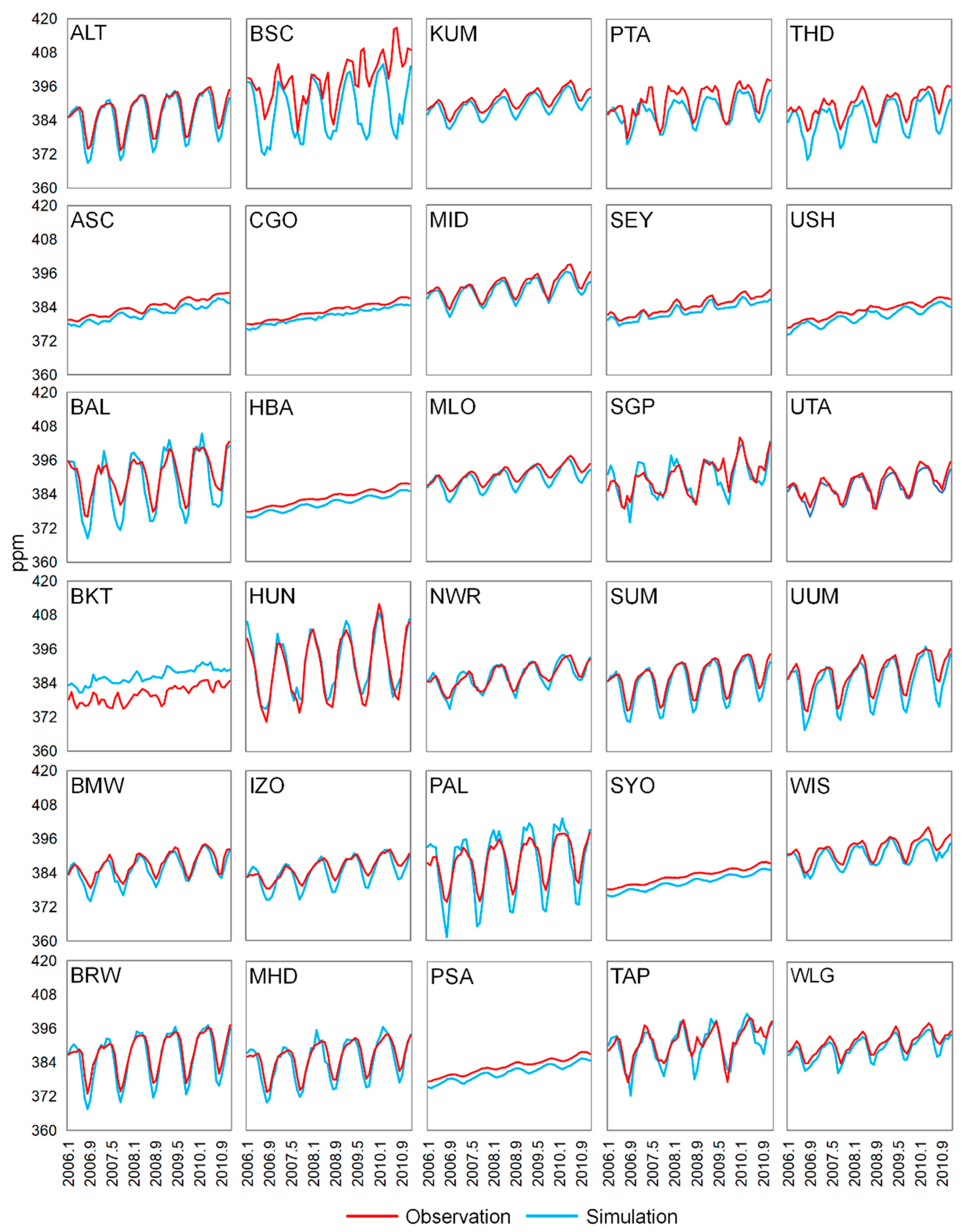
Figure 3.
(a) GEOS-Chem simulated annual surface CO2 concentration.; (b) Average annual growth rate of surface CO2 concentrations simulated by GEOS-Chem.
Figure 3.
(a) GEOS-Chem simulated annual surface CO2 concentration.; (b) Average annual growth rate of surface CO2 concentrations simulated by GEOS-Chem.
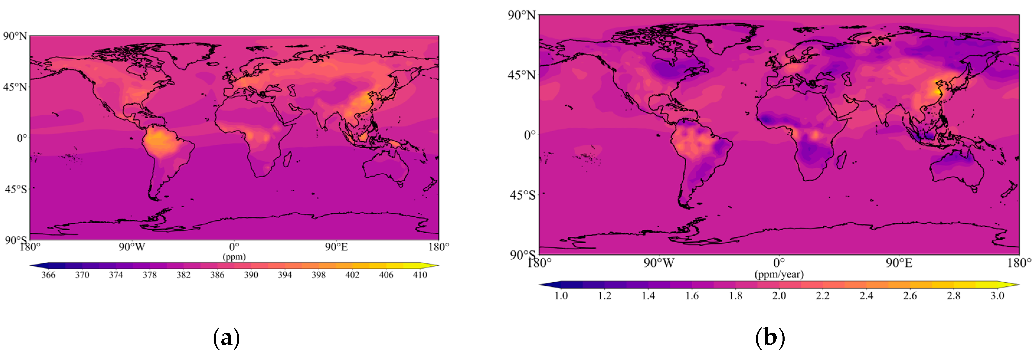
Figure 4.
Average annual global surface CO2 concentrations simulated by GEOS-Chem.

Figure 5.
Total global CO2 fluxes of eight different sources and sinks.
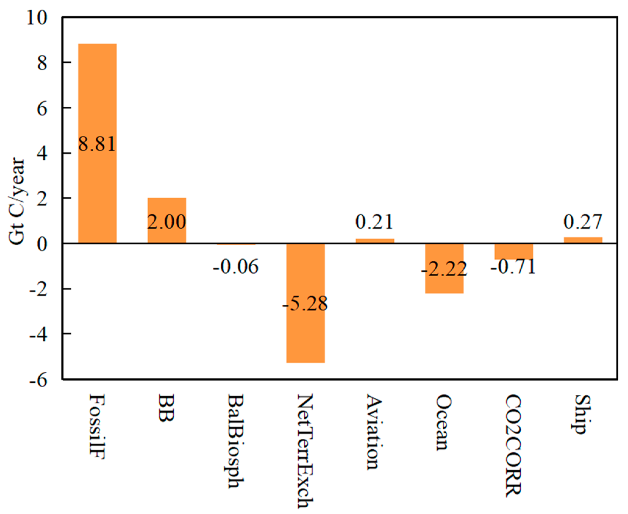
Figure 6.
(a) Fossil fuel carbon emissions; (b) Surface atmospheric CO2 concentrations affected by fossil fuel emissions.
Figure 6.
(a) Fossil fuel carbon emissions; (b) Surface atmospheric CO2 concentrations affected by fossil fuel emissions.
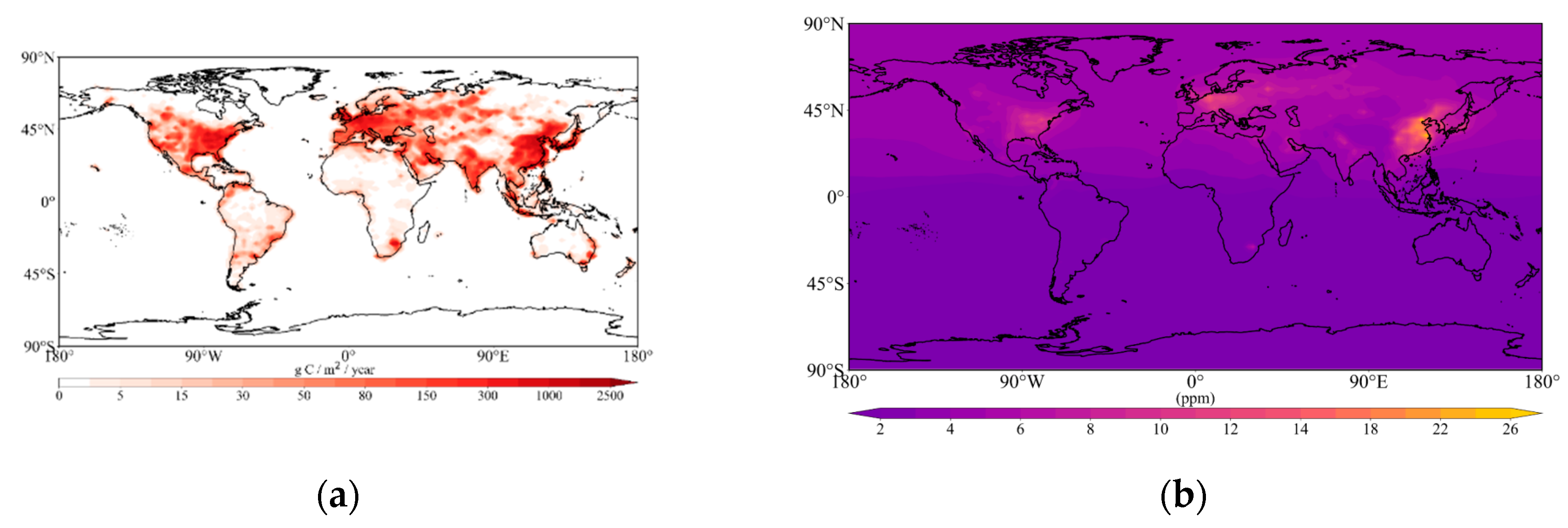
Figure 7.
(a) Carbon emissions from biomass burning; (b) Surface atmospheric CO2 concentration affected by biomass burning emissions.
Figure 7.
(a) Carbon emissions from biomass burning; (b) Surface atmospheric CO2 concentration affected by biomass burning emissions.
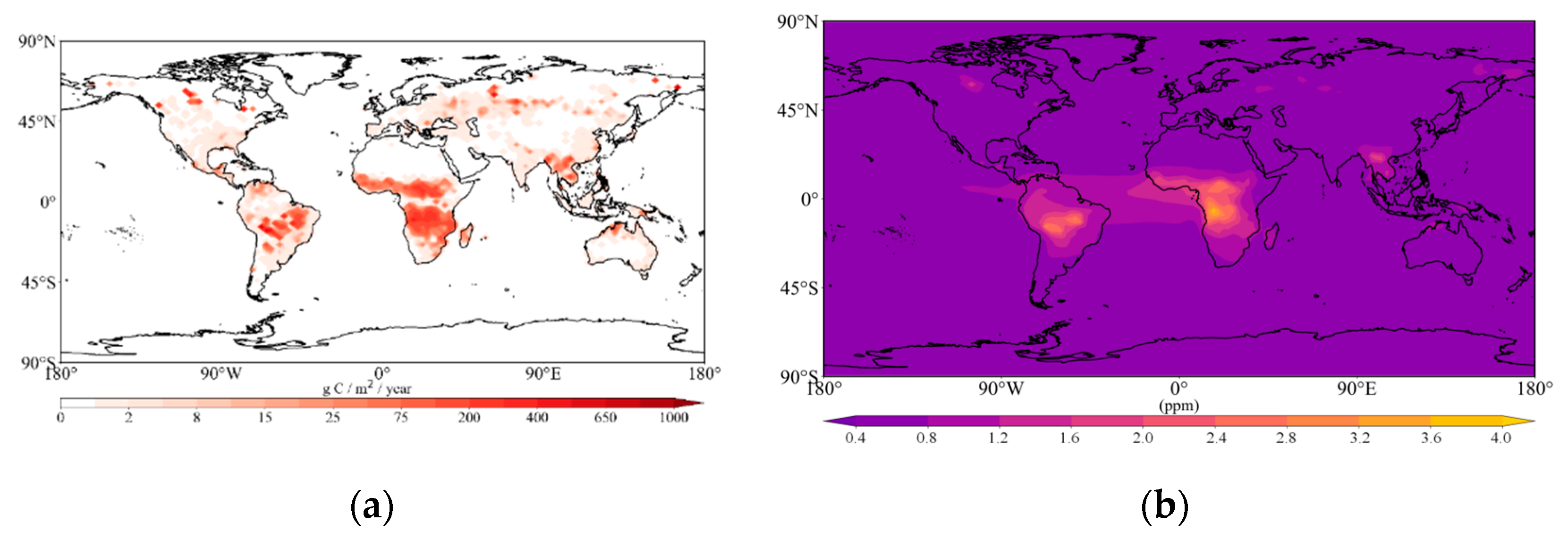
Figure 8.
(a)-(d) Balance biosphere carbon flux in four seasons; (e)-(h) Surface atmospheric CO2 concentrations influenced by balanced biosphere in four seasons.
Figure 8.
(a)-(d) Balance biosphere carbon flux in four seasons; (e)-(h) Surface atmospheric CO2 concentrations influenced by balanced biosphere in four seasons.
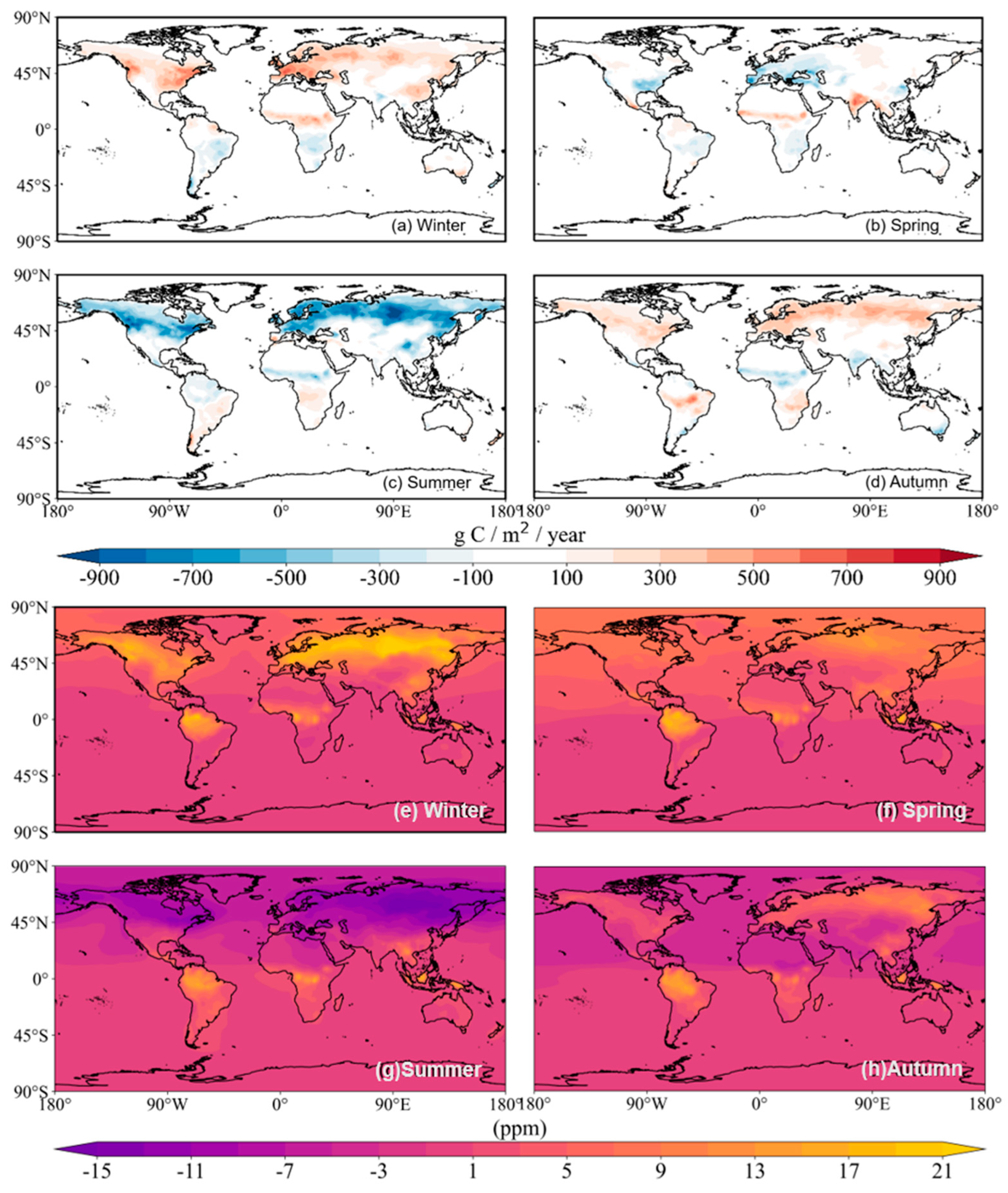
Figure 9.
(a) Net terrestrial exchange; (b) Surface atmospheric CO2 concentrations influenced by net terrestrial exchange in four seasons.
Figure 9.
(a) Net terrestrial exchange; (b) Surface atmospheric CO2 concentrations influenced by net terrestrial exchange in four seasons.
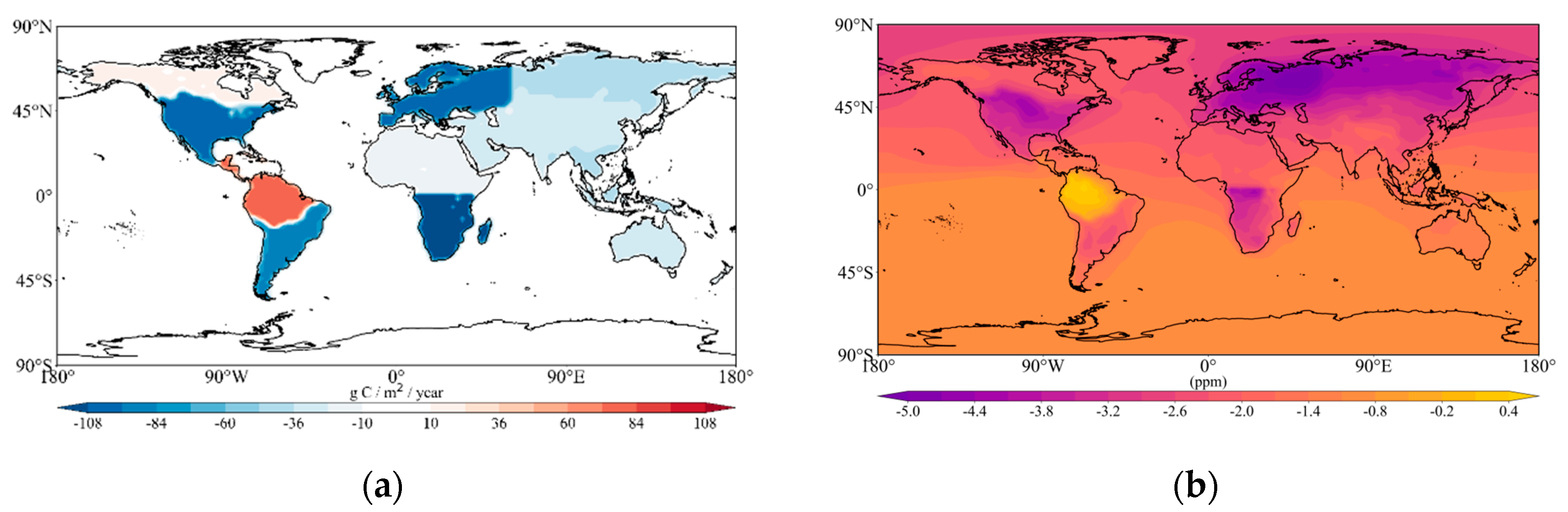
Figure 10.
(a) Carbon emissions from ship; (b) Surface atmospheric CO2 concentrations affected by ship emissions.
Figure 10.
(a) Carbon emissions from ship; (b) Surface atmospheric CO2 concentrations affected by ship emissions.
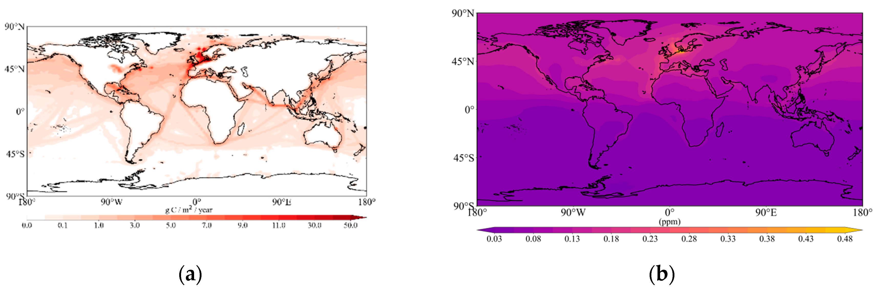
Figure 11.
(a) Carbon emissions from aviation; (b) Average atmospheric CO2 concentrations from different layers affected by aviation emissions.
Figure 11.
(a) Carbon emissions from aviation; (b) Average atmospheric CO2 concentrations from different layers affected by aviation emissions.
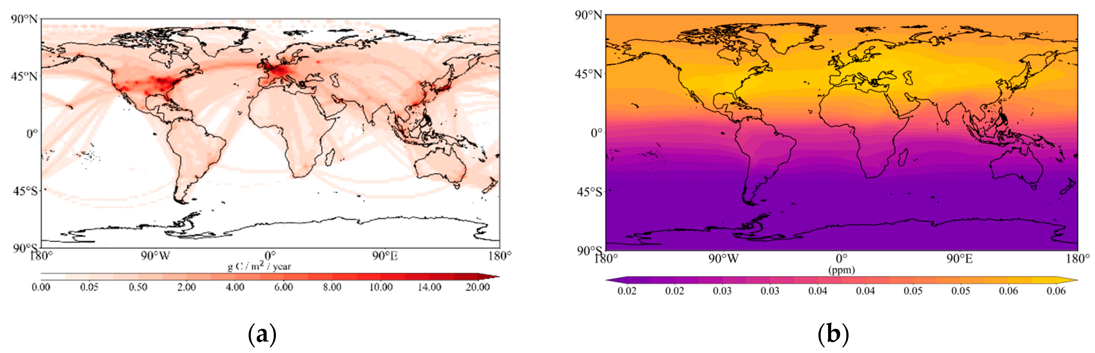
Figure 12.
(a) Ocean exchange carbon fluxes; (b) Surface atmospheric CO2 concentrations influenced by ocean exchange.
Figure 12.
(a) Ocean exchange carbon fluxes; (b) Surface atmospheric CO2 concentrations influenced by ocean exchange.
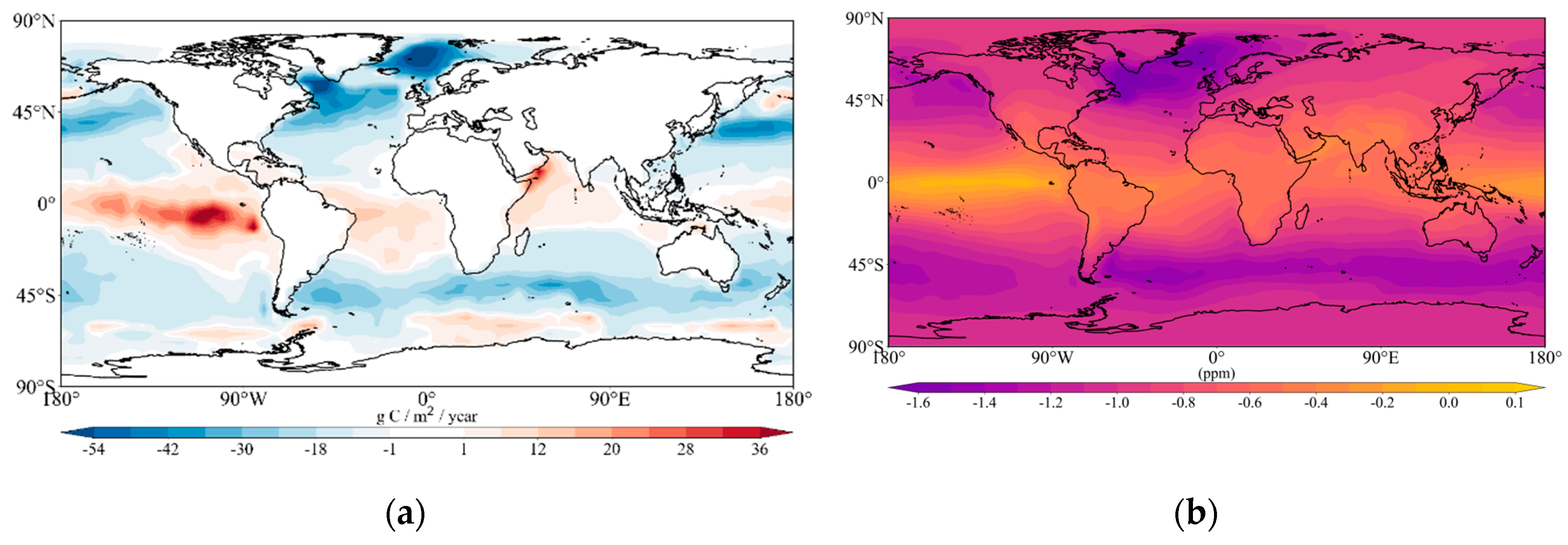
Figure 13.
(a) Chemical sources carbon fluxes; (b) Surface atmospheric CO2 concentrations influenced by chemical sources
Figure 13.
(a) Chemical sources carbon fluxes; (b) Surface atmospheric CO2 concentrations influenced by chemical sources
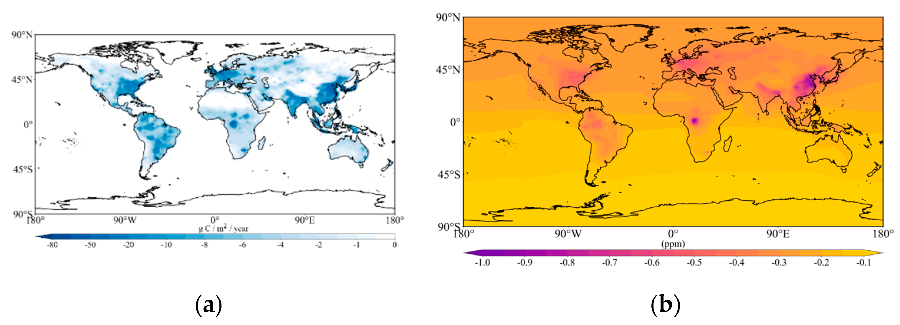

Table 1.
List of CO₂ emission inventories used in the GEOS-Chem simulations in this study.
| Flux Type | Inventory Name Abbreviation |
Description | Spatial | Temporal | References |
|---|---|---|---|---|---|
| Biomass Burning | QFED | Quick Fire Emissions Database for 2006-2010 | 0.1° × 0.1° | Daily | [13] |
| Fossil Fuel | ODIAC | Open source Data Inventory for Atmospheric CO₂ for 2006-2010 | 1° × 1° | Monthly | [14] |
| Ocean Exchange | Scaled oceanexchange | Scaled ocean exchange for 2006-2010 | 4° × 5° | Monthly | [15] |
| Balanced Biosphere | SIB3 | Balanced Net Ecosystem Production (NEP) CO₂ for 2006-2010 | 1° × 1.25° | 3-hourly | [16] |
| Net Terrestrial Exchange | TransCom climatology |
TransCom net terrestrial biospheric CO₂ fixed in 2000 | 1° × 1° | Fixed | [17] |
| Ship | CEDS | Community Emissions Data System for 2006-2010 | 0.5° × 0.5° | Monthly | [18] |
| Aviation | AEIC | Aircraft Emissions Inventory Code fixed in 2005 | 1°×1° | Monthly | [19] |
| Chemical Source | CO₂ Chemical Source | CO₂ chemical production from carbon species oxidation fixed in 2004 | 2°×2.5° | Monthly | [20] |
Table 2.
Simeulation test.
| Flux Type | Inventory Name Abbreviation |
Experiments 1 | ||||||||
|---|---|---|---|---|---|---|---|---|---|---|
| BASE | no_FF | no_BB | no_BalB | no_NTE | no_S | no_A | no_O | no_CS | ||
| Fossil Fuel | FF | + | – | + | + | + | + | + | + | + |
| Biomass Burning | BB | + | + | – | + | + | + | + | + | + |
| Balanced Biosphere | BalB | + | + | + | – | + | + | + | + | + |
| Net Terrestrial Exchange | NTE | + | + | + | + | – | + | + | + | + |
| Ship | S | + | + | + | + | + | – | + | + | + |
| Aviation | A | + | + | + | + | + | + | – | + | + |
| Ocean Exchange | O | + | + | + | + | + | + | + | – | + |
| Chemical Source | CS | + | + | + | + | + | + | + | + | – |
1 "+" indicates that the emission list is enabled, and "-" indicates that the emission list is disabled.
Table 3.
Comparison of simulated XCO2 and GOSAT XCO2 on a monthly basis.
| Time | Sample Size | Simulated Mean (ppm) |
Observed Mean (ppm) |
Simulated Standard Deviation(ppm) | Observed Standard Deviation(ppm) | RMSE (ppm) |
Correlation Coefficient |
|---|---|---|---|---|---|---|---|
| Jan | 6407 | 385.48 | 387.24 | 1.36 | 1.84 | 2.15 | 0.74 |
| Feb | 5456 | 386.03 | 387.63 | 1.59 | 1.92 | 1.98 | 0.80 |
| Mar | 8285 | 386.86 | 388.27 | 1.88 | 2.11 | 1.78 | 0.86 |
| Apr | 8583 | 387.83 | 389.27 | 2.00 | 2.34 | 1.81 | 0.89 |
| May | 9396 | 387.88 | 389.52 | 1.74 | 2.39 | 2.07 | 0.86 |
| Jun | 10609 | 386.94 | 388.90 | 1.32 | 1.74 | 2.39 | 0.62 |
| Jul | 11704 | 385.47 | 387.57 | 2.04 | 2.07 | 2.48 | 0.80 |
| Aug | 14258 | 385.30 | 387.36 | 1.64 | 1.84 | 2.34 | 0.81 |
| Sep | 14166 | 385.44 | 387.51 | 1.16 | 1.33 | 2.33 | 0.64 |
| Oct | 14369 | 385.97 | 388.10 | 0.58 | 1.14 | 2.36 | 0.44 |
| Nov | 13207 | 386.30 | 388.39 | 0.42 | 1.03 | 2.32 | 0.28 |
| Dec | 8796 | 386.70 | 388.78 | 0.91 | 1.40 | 2.35 | 0.64 |
| Yr | 125236 | 386.26 | 388.18 | 1.67 | 1.89 | 2.25 | 0.79 |
Disclaimer/Publisher’s Note: The statements, opinions and data contained in all publications are solely those of the individual author(s) and contributor(s) and not of MDPI and/or the editor(s). MDPI and/or the editor(s) disclaim responsibility for any injury to people or property resulting from any ideas, methods, instructions or products referred to in the content. |
© 2025 by the authors. Licensee MDPI, Basel, Switzerland. This article is an open access article distributed under the terms and conditions of the Creative Commons Attribution (CC BY) license (http://creativecommons.org/licenses/by/4.0/).
Copyright: This open access article is published under a Creative Commons CC BY 4.0 license, which permit the free download, distribution, and reuse, provided that the author and preprint are cited in any reuse.


