
Submitted:
02 February 2025
Posted:
04 February 2025
You are already at the latest version
Abstract
Recent studies have revealed a rise in extreme heat events worldwide, while extreme cold has shown a decline. It is highly likely that human-induced climate forcing will double the risk of severe heat waves by the end of the century. Although extreme heat is expected to have greater socioeconomic impacts than cold extremes, the latter contributes to a wide range of adverse effects on the environment, various economic sectors and human health. People can somewhat adapt to extreme temperatures when they experience repeated heat and cold waves, but these extreme events can have more severe health consequences when they occur earlier in the respective season or last unusually long. A few studies have re-cently analyzed extreme heat events on a European scale using the excess heat factor (EHF) that accounts for short-term acclimatization. This approach is also analogously ap-plicable to extreme cold events by employing the excess cold factor (ECF). The present re-search aims to evaluate the spatiotemporal variations of extreme cold events in South-eastern Europe through the intensity-duration model developed for quantitative assessment of cold weather in Bulgaria. We demonstrate the suitability of indicators based on minimum temperature thresholds to evaluate the severity of extreme cold events in the period 1961–2020 both at individual stations and Köppen’s climate zones using daily temperature data from 70 selected meteorological stations. The ability of the used intensity-duration model to estimate the severity of extreme cold events has been compared with the ECF severity index on a yearly basis.
Keywords:
minimum temperature thresholds
; extreme cold event
; excess cold factor
; Köppen’s climate zones
; Southeastern Europe
1. Introduction
Over millions of years, the climate system behavior has been dominated by natural fluctuations at different time scales, but during the last 150 years, anthropogenic forcing substantially influenced natural variability [1,2]. In the context of climate change scenarios, an increase in global temperature of 2 °C compared to the pre-industrial period is considered an upper limit above which the risk of dangerous and irreversible climate shifts increases sharply [3,4,5]. Given that the rise in global temperature has already exceeded half of this limit, it can be crossed in the next 20-30 years [1,6,7]. Heat and cold waves are among the most impactful large-scale natural phenomena strongly related to climate change. Prolonged periods of extreme temperatures cause thermal stress and may have adverse or fatal effects on human health [8,9,10]. They directly and indirectly influence labor productivity and well-being [11,12]. Extreme temperatures considerably increase the risk of energy supply outages and damage to the infrastructure [13,14]. They can even represent a limiting factor for agriculture in the changing climate due to the amplified likelihood of frosts and prolonged hot spells during the vegetation period [15,16,17].
Against the background of the expected rise in global temperatures, a decrease in cold extremes seems intuitively sound [1,18,19]. The impact of heat waves will significantly exceed those of cold waves till the end of the century. Across all studies, the authors point out the multifold increase in the duration, frequency and intensity of future extreme heat events as highly likely [1,20,21]. In Europe, since the beginning of the century, heat waves have caused more deaths than all other natural disasters [22]. Schär et al. [23] revealed that the record summer of 2003 cannot be explained by solely shifting the mean of the temperature distribution to higher temperatures but with an additional increase in variability. The changed shape of the temperature distribution contributes to the occurrence of more hot extremes but also suggests that future cold extremes cannot be inferred from changes in mean and variance alone [24,25]. In this sense, recent severe cold events in Europe, such as in 2010, 2012 and 2017, have received particular attention [26,27,28,29]. Cold extremes would still be possible in the current climate [30,31] and will continue to impact various socioeconomic sectors, particularly healthcare, due to the complex relationship between human thermal adaptation capability and warming rates. Recent studies indicate increased tolerance to hot weather and significant differences among age groups in response to cold events [10,32,33,34,35].
After the deathly European heatwave of 2003, heat extremes have become a priority topic in climate change research [36]. Despite remarkable progress in recent years and the apparent upward trend in heat wave intensity, duration, frequency and spatial extent, there is still no universally agreed definition for this phenomenon [37,38,39]. Therefore, criteria and procedures for identifying extreme heat at a national level are very diverse [40,41]. This lack of consensus also extends to cold wave definitions and warnings.
An extreme event occurs when a climate variable is above or below a defined threshold at the upper or lower end of the range of its observed values. This threshold can be calculated as absolute (fixed) or relative (percentile-based) value [1]. Since around 60% of the national weather services that have criteria for heat/cold waves use absolute thresholds when considering heat and cold events, the World Meteorological Organization (WMO) Task Team for the Definition of Extreme Weather and Climate Events (TT-DEWCE) specified the term heatwave as unusually hot weather relative to the local climate lasting at least two consecutive days in the warmest months of the year. Similarly, cold waves denote unusually cold weather during the cold season, lasting at least two days and often preceded by a rapid and marked drop in air temperature caused by the advection of cold air [37]. These definitions allow flexibility in reporting heat/cold events when different criteria and approaches are used (from a simple descriptive approach to classification schemes based on local climatology, human perception of heat/cold stress, or increased mortality risk [41]).
Extreme heat events can be quantitatively assessed by indices describing their particular characteristics [42,43,44], and similar indices can be defined analogously for extreme cold events (ECEs). Some basic requirements should be satisfied when developing indices of heat and cold extremes [45]. Generally, they should be suitable for various economic and social sectors or climates, but they should also allow comparative analysis. Indices should be easy to understand, calculate, represent and forecast. They should give the public and decision-makers direct, meaningful information on the expected severity of the heat and cold waves. The advantage of percentile-based indices is their global applicability, but fixed-threshold indices are indispensable when monitoring high or low temperatures, which negatively impact health or the economy, is important [39]. Thresholds can be combined to define cascading schemes accounting for the spatiotemporal evolution of extreme events [46]. The rarity of heat and cold extremes should be determined relative to a standard climate period, so a balance must also be found between the threshold levels and the number of events identified as extreme [37,43].
The most popular and widely used set of climate indices consists of 27 core climate change indices (17 temperature-based) developed by the WMO Expert Team on Climate Change Detection and Indices (ETCCDI), initially designed for scientific purposes (http://etccdi.pacificclimate.org/list_27_indices.shtml) (accessed on 28 January 2025). Subsequently, the WMO Expert Team on Sector-specific Climate Indices (ET-SCI) expanded this list to include custom-defined threshold indices and new heat/cold wave indices based on definitions accounting for excessive heat/cold accumulation and short-term thermal acclimatization (https://climpact-sci.org/indices) (accessed on 28 January 2025). In recent years, there has been growing attention to indices based on health-related definitions, particularly for early warning purposes in large cities [41,47,48].
The region around the Mediterranean basin, including Southeastern Europe, is among the most vulnerable to climate change, experiencing more frequent and intense severe weather events and heat extremes [1,49,50,51]. Besides heat waves, cold events have also been the subject of various regional studies in recent decades. Tringa et al. [52] conducted an extensive climatological and synoptic analysis of winter cold spells in the Balkan Peninsula from 1961 to 2019. They found a decreasing trend in the frequency of cold spells toward the end of that period. Planchon et al. [27] performed a multi-scale agroclimatic analysis for Romanian vineyards in the meteorological context of the early 2012 European cold wave. Demirtaş [28] analyzed the anomalously cold January 2017 in Southeastern Europe through the connection between cold spells and atmospheric blocking using an objective coldwave indicator and a two-dimensional blocking indicator. Kostopoulou [53] investigated the potential effects of the January 2017 cold spell on mortality attributed to cardiovascular disease. Faranda et al. [54] conducted an attribution study on the winter storm Filomena in 2021, marked by historic snowfalls in the inland regions of the Iberian Peninsula and a prolonged 14-day cold spell. Kysely et al. [55] demonstrated that cold stress significantly impacts mortality in Central Europe, representing a public health threat comparable to that posed by heat waves. Díaz-Poso et al. [56] analyzed climate change scenarios using simulations from the EURO-CORDEX project, applying the Excess Cold Factor (ECF) index for the Iberian Peninsula and the Balearic Islands. Their results indicated that despite the expected decrease in cold waves, they would continue to pose a serious local threat due to the population’s acclimatization to higher temperatures. Piticar et al. [57] found substantial changes in the indices of excess heat/cold factor and concluded that heat waves have become more frequent, longer, and more intense, while cold waves have become less frequent but more intense in Romania.
The present study can be viewed as continuing previous research on spatiotemporal variations of hot spells in Southeastern Europe [58]. The indicators proposed here for quantitative assessment of cold-weather phenomena could be helpful in sector-specific climate assessments. The study aims to test the suitability of developed indicators for an overall analysis of ECEs in Southeastern Europe. The ability of the cold spell duration indicator to detect extreme cold events has also been examined and compared with the ECF-based indices.
2. Data and Methods
We consider the same domain over Southeastern Europe (SEE), with coordinates 35°N–50°N and 15°E–30°E (the red frame in Figure 1), as in the previous study [58]. This area almost entirely falls within the Mediterranean region, as defined by the Mediterranean Experts on Climate and Environmental Change (MedECC) [59]. According to the updated Köppen-Geiger classification [60], the European part of the Mediterranean region mostly belongs to the midlatitude temperate climate zone, comprising Mediterranean climate types with a dry hot/warm summer (Csa/Csb) and large areas with no dry hot/warm summer (Cfa/Cfb), but also areas with continental hot/warm/cold climates (Dfa/Dfb/Dfc) in the north [61].
The same dataset, developed for evaluating the spatiotemporal variations of extreme heat events in the period 1961-2020 in SEE [58], is used here to investigate extreme cold events. This dataset consists of daily maximum and minimum air temperature data from 70 selected meteorological stations covering the study area relatively evenly (Figure 1). Data from 12 stations of the national meteorological network of Bulgaria are provided by the National Institute of Meteorology and Hydrology (NIMH). Data from stations outside Bulgaria were downloaded from three freely available sources: the European Climate Assessment and Dataset (ECA&D) project [62], the U.S. National Climatic Data Center (NCDC) Global Historical Climatology Network daily dataset (GHCNd) [63], and the U.S. National Centers for Environmental Information (NCEI) Global Surface Summary of the Day (GSOD) dataset [64]. Most stations have altitudes below 500 m and are distributed across four Köppen-Geiger climate zones [60] – Cfa (25%), Cfb (34%), Csa (21%) and Dfb (20%). The stations’ metadata are presented in Appendix A, Table A1.
We have demonstrated in the previous study the suitability of climatologically justified for Bulgaria thresholds of daily maximum temperature (32, 34, 36, 38 and 40 °C) and corresponding duration thresholds (6, 5, 4, 3 and 2 consecutive days) to classify extreme heat events in SEE. Given that the prevailing in Bulgaria Köppen’s climate subtypes (Cfa and Cfb) is almost 60% of the whole domain, we expect to obtain a sufficiently accurate picture of changes in cold extremes in the period 1961-2020 by combining thresholds for daily minimum temperature and cold spell duration, using the same dataset and methodology as in the estimation of extreme hot spells.
The threshold indicators defined in [58] were developed using statistical modeling of daily maximum air temperature data from 36 stations, including the 12 stations shown in Figure 1, representative of the non-mountainous regions in Bulgaria with at least 80 years of observations in the period 1931-2020, referred to as BG36 hereafter (stations’ metadata are presented in Appendix A, Table A2). In the present study, we strictly followed this approach and used the same meteorological stations to ensure the methodologically consistent analysis of minimum temperatures and extreme cold events. Data on daily minimum air temperature from the BG36 dataset were processed to obtain the distribution of minimum temperatures and corresponding quantiles characteristic of the climate in the country.
Data processing involved several steps: 1) construction of empirical distributions of annual minimum temperatures for 1931–1980 (the period is considered as less affected by global warming [2,65,66]); 2) calculation of quantiles corresponding to return periods 2, 5, 10, 20 and 50 years by fitting the Generalized Extreme Value (GEV) distribution to data, accounting for nonstationarity of time series [67]; 3) determination of appropriate thresholds for daily minimum temperature (tn); 4) determination of cold spells duration thresholds for the period 1961–2020 at the different tn-thresholds.
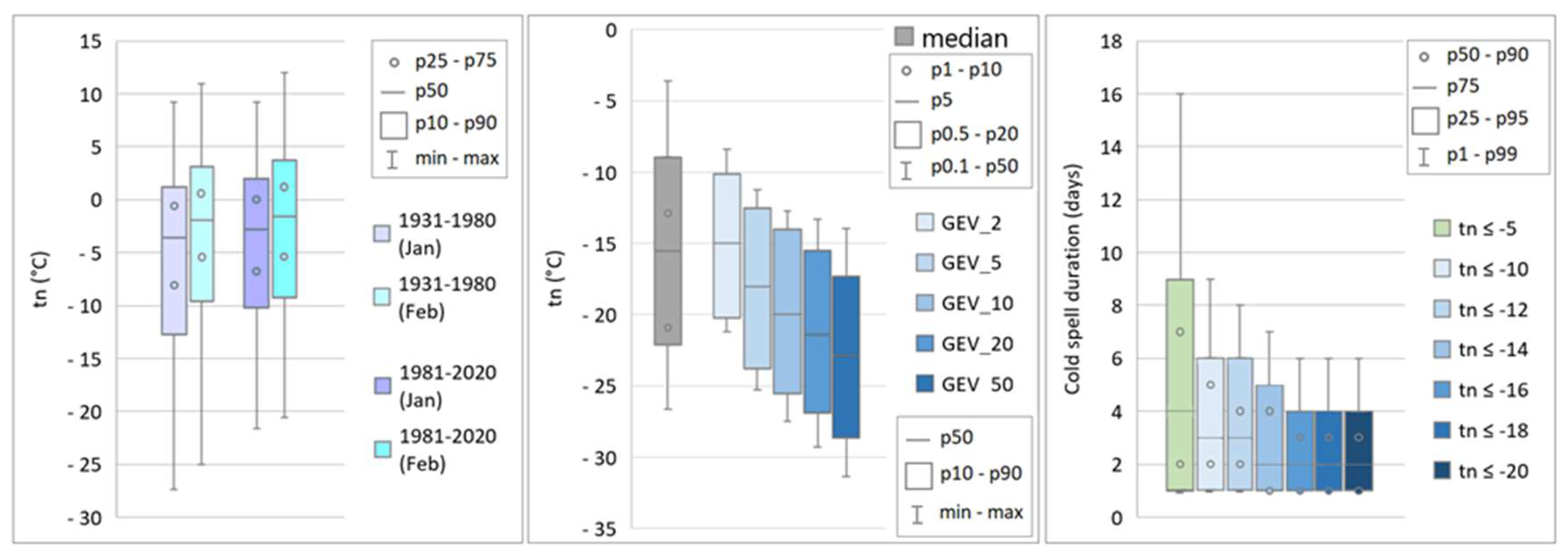
Until 1980, daily minimum temperatures in the coldest months in Bulgaria (January and February) fall mainly into the range from -27.4 °C to 11 °C across the selected stations, and the absolute minima are typically between -30.8 °C and -22.5 °C. From the estimated 2-, 5-, 10-, 20- and 50-year return levels by the GEV model (Figure 3, middle panel), the set of thresholds (-10, -12, -14, -16, and -18 °C) have been chosen in such a way to be achievable in more than 80% of stations. During the second period (1981–2020), a substantial shift of tn-distributions toward higher values is observed (Figure 3, left panel). Therefore, the cold spell duration thresholds were determined for the period 1961–2020 to provide a reliable analysis of ECEs in the contemporary climate. Cold spells last 2-3 days most frequently, and the 90th percentile varies between 3 and 5 days.
Assuming that the research focuses on applying threshold indicators to analyze extreme cold in a climatically diverse region, such as SEE, we explored the minimum temperature features by Köppen-Geiger climate zones. First, we calculated empirical quantiles, corresponding to the return periods used here, from the time series of annual minimum temperatures (1961–2020) for all 70 stations. As seen in the left panel of Figure 2, the median values remain well below the chosen tn-thresholds (blue dots in the chart). This suggests that more frequent and longer cold spells will be detected in at least 50% of the stations, determining the proposed cold spell duration indicator as an indicator of moderate extremes [42]. The chosen thresholds are well-suited for more than 70% of stations in the domain but not for stations in the Csa climate zone. The thorough analysis showed that for 2-year return periods, -5 °C is achievable in 35% of the Csa stations and 85% of all stations, while -20 °C is achievable in around 10% of stations. The right panel of Figure 2 shows the calculated percentiles of the lower tail of distributions of daily minimum temperatures by stations in the four climate zones as box-plot diagrams. One can see that only percentiles below the 10th, usually used in ECE definitions, fall within the range from -20 °C to -5 °C.
2.1. Climatologically Justified Threshold Indicators
Given the obtained estimates about low temperatures in the studied domain, the cold spell duration indicator was developed based on samples from the BG36 dataset and the extended set of tn-thresholds (-5, -10, -12, -14, -16, -18 and -20 °C). The right panel in Figure 3 shows the distribution of cold spell durations at different tn-thresholds for the period 1961-2020. Duration thresholds were selected as the 90th percentile of the respective distributions: 7 days for tn ≤ -5 °C, 5 days for tn ≤ -10 °C, 4 days for thresholds of -12 °C and -14 °C, and 3 days for thresholds of -16 °C and -18 °C. For cold spells with tn ≤ -20 °C, we selected a minimum duration of 2 days [37]. A recent study on cold waves in the non-mountainous regions of Bulgaria in the period 1952-2011 found that cold events, assessed using the ETCCDI Cold Spell Duration Index (CSDI), mostly last between 6 and 11 days, reaching minimum temperatures between -5 °C and -20 °C [68]. These results confirm that the proposed range of tn-thresholds and the 7-day duration threshold for lowest-intensity cold spells are relevant to capturing the evolution of cold spells in the current climate.
Analogously to the hot weather indicators in [58], three climate indicators of cold weather have been defined:
- Annual number of cold days (ncd-5) – i.e., the annual count of days when tn < -5 °C;
- Maximum number of consecutive cold days (ccd-5) – i.e., the longest continuous calendar period when tn < -5 °C;
- Cold spells duration at different tn-thresholds (csd-5/-10/-12/-14/-16/-18/-20) – i.e., the annual count of days when tn ≤ -5, -10, -12, -14, -16,- 18 and -20 °C for at least 7, 5, 4, 4, 3, 3 and 2 consecutive days, respectively.
The first indicator represents a common measure of unfavorable cold-related conditions during the year. The second indicator delineates the upper bound of the cold weather persistence. The third indicator allows combined (intensity-duration) evaluation of ECEs in seven sevirity categories (very low/low/moderate/elevated/high/very high/extreme). The technology of calculation of the csd indicator allows the separation of events and the analysis of their temporal evolution.
The results are summarized for the SEE domain by the Köppen-Geiger climate zones. The significance and magnitude of trends in proposed indicators were assessed through the non-parametric Mann-Kendall’s test [69] and Sen’s method [70] using the R-package ‘trend’ [71].
Figure 3.
Left panel: Medians of calculated percentiles of tn-distributions by stations for 1931–1980 and 1981–2020. Middle panel: Median of calculated lower percentiles of tn-distributions and 2-, 5-, 10-, 20- and 50-year return levels (estimated by GEV model) by stations for yearly minima (1931–1980). Right panel: Box plot of distributions of cold spells duration at the different tn-thresholds for 1961-2020. The BG36 dataset was used for all calculations.
2.2. Excess Cold Factor (ECF)
Several studies have recently analyzed extreme heat events in Europe and worldwide using the excess heat factor (EHF) that accounts for short-term acclimatization (e.g., [72,73,74,75]). This approach can be analogously applied to extreme cold events by using the excess cold factor [56,76,77,78,79]. ECF measures cold wave intensity at each location with an additional component to account for adaptation [45]. The units of excess cold are °C2 as the ECF is a factorization of two cold indices representing the degree of acclimatization to cold and the climatological significance:
ECIaccl = (Ti + Ti-1 + Ti-2)/3 – (Ti-3 + … + Ti-32)/30
ECIsig = (Ti + Ti-1 + Ti-2)/3 – T05
Ti = (Tmaxi + Tmini)/2
ECF = -ECIsig × min(-1,ECIaccl)
where Ti represents the average daily temperature for day i and T05 is the 5th percentile, calculated within the given base period (1961-1990 in this study); Tmaxi and Tmini are the maximum and minimum temperatures for day i.
ECF is negative (i.e., coldwave is in progress) when ECIsig is negative (because the three-day period is cold in an absolute sense, being below the 5th percentile for daily mean temperature), but additionally, the three-day period is substantially cooler than the preceding 30 days (ECIaccl < -1 °C). Positive values of ECF mean a coldwave is not in progress [45].
The ECF severity (ECFsev) metric permits the comparison of cold wave events and their impacts across the world and can be readily implemented within early warning systems [80]. For given day i, ECF severity is defined as follows:
where ECFp15 denotes the 15th percentile of all negative ECF values calculated for the base period.
ECFsevi = ECFi /ECFp15, if ECFi < 0
ECFsevi = 0, if ECFi ≥ 0
Nairn et al. [80] defined three levels of ECE severity:
- L1 (low-intensity), when 0 < ECFsev < 1;
- L2 (severe), when 1 ≤ ECFsev < 3;
- L3 (extreme), when 3 ≤ ECFsev.
The annual summaries of ECFsev characteristics, such as mean and maximum magnitude and maximum number of consecutive days of excess cold, were calculated by stations and presented by the Köppen-Geiger climate zones.
2.3. Software Products Used in the Research
3. Results and Discussion
In recent years, many studies have focused on the rising temperatures in Europe since the second half of the 20th century. Twardosz et al. [84] found that the rate of increase is almost twice as rapid from 1985 to 2020 as in the whole period after 1951 (0.027 and 0.051 °C/year, respectively). This aligns with our results concerning trends in annual mean temperatures in the examined domain for 1961-2020 and 1985-2020 (0.032 and 0.055 °C/year, respectively) [58]. However, the authors conclude that the rise in temperature during the winter should be considered much less steady than in the summer. Sippel et al. [65] found that the observed rapid increase in cold-season temperatures in the late 1980s was followed by relatively modest temperature trends thereafter, which can be interpreted as a manifestation of internal variability superimposed upon the long-term warming component.
Table 1 shows magnitudes of trends in annual mean (Ta), annual mean minimum (Tmn) and annual minimum temperatures (Tn) in the period 1961-2020 by climate zones. The largest magnitudes are obtained for Tn in the Cfb and Dfb climate zones. Most stations with larger trend magnitudes are located in the central and northern parts of the SEE domain. Unlike Ta, with statistically significant trends for all stations, the percentage of stations with significant trends in Tmn and Tn varies between 82% (Cfa) and 100%(Cfb) for Tmn and between 6-7% (Cfa and Csa) and 50%(Cfb) for Tn.
Figure 4 illustrates the long-term variation of the averaged by climate zone indicators ncd-5 and ccd-5 (calculated separately for each station), which reveals a downward tendency in all climate zones except for Csa. Both indicators show a statistically significant negative trend for 18% of stations in Cfa and up to 88% in the Cfb climate zone (Table 2). The average magnitude of the ncd-5 trends ranged between -3.1 (Dfb and Cfb) and -1.5 (Cfa) days/10 years, and the maximum magnitude of -4.5 days/10 years was reached in the Cfb climate zone. The ncd-5 maxima vary by stations between 0 and 118 days, with lower values occurring in coastal Csa stations. Around 50% of maxima were recorded in 1963, 10% in 1985, and 6% in 1987 and 1993.
The average magnitudes of the ccd-5 trend ranged between -1.0 (Cfb) and -0.4 (Cfa) days/10 years, and the maximum magnitude of -1.3 days/10 years was reached in the Cfb climate zone. The ccd-5 maxima vary by stations between 0 and 50 days, with the lowest values occurring again in Csa stations. The distribution of maxima by years differs from this one of ncd-5 – most of them have occurred again in 1963 (41%) and 1985 (13%), but also in 2012 (10%), 1964 (7%) and 1996 (6%).
The comparison of multiyear means of ncd-5 and ccd-5 for 1961–1990 and 1991–2020 is shown in Figure 5. The number of cold days decreased during the second period by 14% and 21% in the Dfb and Cfb climate zones, respectively, but there was no substantial change in the Cfa and Csa zones. The most significant change in ccd-5, both in absolute terms (-2.4 days) and as a percentage change (-24%), was registered in the Cfb climate zone.
Figure 6 presents the evolution of the cold spell duration indicator (csd) by categories, averaged by climate zones. The highest values for csd-5 were reached in 1963 (Dfb and Cfb) and 1985 (Cfa and Csa). The csd indicator distinguished the severity of extreme cold weather well in most of the SEE domain and marked some extremely severe cold events in the Csa climate zone, such as in 1968, 1985 and 2001 [85,86]. The calculated average trend magnitudes decreased with the csd-category increasing, varying from -2.7 to -0.2 days/10 years in Dfb and from -1.7 to -0.3 days/10 years in Cfb climate zone (Table 2).
Our results regarding the relatively weak-expressed trends in cold weather indicators can be viewed in the context of the less steady rise in winter temperatures compared to the rapid increase in summer temperatures in Europe [84]. Moreover, a recent study shows that little has changed with cold extremes since 1990, despite the intuitive suggestion that Northern Hemisphere cold extremes would become less intense and frequent not only with global warming but as the Arctic warms at an accelerated pace [87]. Concerning SEE, these findings align with the research of Buric and Doderovic [88], which reported a decrease in the number of cold nights (defined as days when tn < 10th percentile) during winter in Montenegro. This reduction varies from 0 to -2.5 days/10 years for stations with altitudes below 800 m, but it is statistically insignificant at 9 out of 11 stations.
Temperature thresholds underlying the proposed method for detecting and classifying ECEs through intensity-duration model include some physiological and technological limits, which crossing could have significant adverse health and economic consequences, such as increasing morbidity and mortality rates in cardiovascular, respiratory and some other illnesses [10,89], agricultural damage [15,17,90] and disruptions in energy production and supply [13,91]. On the other hand, ECF severity is helpful as an exposure index that scales well against human health impact [80] and an extreme cold indicator in climate studies [45]. Therefore, we choose the ECFsev index to assess the suitability of the proposed threshold indicators. First, we examine the consistency between the most extended periods of consecutive cold days on a yearly basis, calculated as ccd-5 and ccd-ECF (where the latter is defined as the longest period of excess cold, ECFsev > 0) using the SEE dataset. Long-term variations of ccd-5 and ccd-ECF, averaged by climate zones, are shown in Figure 7. It is evident that the -5 °C threshold is rather strict for Csa but quite soft for Dfb climates when assessing the excess cold that populations may experience. However, the correlation between ccd-5 and ccd-ECF remains high enough, even for the Csa zone.
During the studied period, each station reached a daily value of ECFsev ≥ 3 at least once. The absolute maxima of ECFsev range from 3 to 11.3, with the highest value recorded in December 2001 in Larissa, Greece. The number of days with excess cold varies slightly by station (12 to 17 days per year). Approximately 81% of the calculated daily values of ECFsev are below 1.0 (severity level L1). Excess-cold days mainly occurred in January (45%) and February (25%). The estimated statistically significant trend magnitudes for ccd-ECF vary between -0.4 and -1.0 days/10 years, affecting 6-7% of stations in Cfa and Csa climates, 21% in Dfb and 75% in Cfb climates.
The indices averaged over the domain (ccd-5d and ccd-ECFd) indicate a strong linear relationship (r = 0.958). According to the definition of ccd-5, the longest cold period of the year falls typically into the coldest winter months, January and February. Thus, an interesting classification of winter severity can be derived by the scatter plot of ccd-ECFd vs. ccd-5d, accounting for the averaged yearly maxima of ECFsev (Figur 8). Most years with mild winters (severity level L1) in SEE are associated with ccd-5d below 7 days. For years with severe winters (L2), ccd-5d is usually between 7 and 10. A few winters have prolonged cold periods exceeding 13 days, with ECFsev above 2.5, categorizing them as significantly more severe. The only winter with the highest severity level (L3) is that in 1963, also characterized by the most prolonged cold period (ccd-5d = 18 days). Generally, this categorization of winters is confirmed by various regional analyses and studies [e.g., 85,86,92,93].
Figure 9 presents an estimate of extreme cold weather in SEE based on the average ECFsev, calculated for 1961-1990 and 1991-2020 on a yearly basis, over all periods of at least 7 days with tn ≤ -5 ℃ (in such a way being synchronized with the lowest severity category of the cold spell duration indicator, csd-5).
The results show that despite the decreasing number of ECEs in recent decades, the severity of cold weather in SEE has changed little regarding the excess cold that populations may experience. Percentage changes indicate that the Cfb climate zone is the most affected by regional warming.
The detailed comparison between yearly maxima of csd-categories (denoted by C1 to C7) and ECFsev levels demonstrated good spatiotemporal conformity, as seen in the left panel of Figure 10. Although the relationship between them is complex, the percentage distribution of different categories by severity levels shows that the categories from C4 to C6 are more strongly related to L2. In contrast, the other categories are fuzzified between neighbor ECFsev levels: C1 category mainly corresponds to L1, and over 30% of cases in C7 category align with L3 (Figure 10, right panel).
5. Conclusions
The subject of our study is the cold-weather climate phenomena related to the prolonged retention of extreme cold in Southeastern Europe. Although the cold spells are typical for the cold season in SEE, the research on their spatio-temporal changes is somewhat neglected compared to the extreme heat. This study can be viewed as a continuation of our previous work concerning the development of criteria and indicators for quantitative assessment of hot spells [58]. We used the same methodologies and datasets to investigate the spatiotemporal variations of extreme cold in the period 1961-2020. Three threshold indicators based on daily minimum temperature, presenting the unfavorable cold-season thermal conditions (ncd-5), cold weather persistence (ccd-5) and combined intensity-duration characteristic of cold spells in seven categories (csd-5/-10/-12/-14/-16/-18/-20) were analyzed and summarized by the zones of the Köppen-Geiger climate classification. All three indicators show statistically significant decreasing trends (p < 0.05, Mann-Kendall method) during the period 1961-2020 in the areas with typically cold winters in the northern and central parts of the studied domain. Comparing the two 30-year periods (1961-1990 and 1991-2020), we found that cold days decreased by 14% and 21% in the Dfb and Cfb climate zones, respectively, but there was no substantial change in the Cfa and Csa zones. The results show good consistency between the indicator of consecutive cold days (ccd-5) and the yearly longest period of excess cold. We presented the classification of winter severity in the SEE domain based on the averaged yearly maxima of ccd-5 and ECFsev. Excess-cold days in SEE are typically 12-17 per year, occurring mainly in January (45%) and February (25%). Most years with mild winters (severity level L1) in SEE are associated with a short retention of cold weather (below 7 days). A few winters have more prolonged cold periods exceeding 13 days, with ECFsev above 2.5, categorizing them as significantly more severe. The only winter with the highest severity level (L3) is that in 1963, also characterized by the most prolonged cold period (18 days).
Given the increased mortality risk, agricultural losses and disruptions in the energy sector linked to prolonged cold weather and extremely low temperatures, we demonstrated the suitability of the proposed intensity-duration model to classify extreme cold events in the studied domain based on the set of minimum temperature thresholds (-5, -10, -12, -14, -16, -18 and -20 °C) and corresponding duration thresholds (7, 5, 4, 4, 3, 3 and 2 consecutive days). The detailed comparison between categories of the cold spell duration indicator and yearly maxima of the ECFsev levels demonstrated good spatiotemporal conformity.
As far as we know, no survey has been conducted on the various aspects of using threshold indicators for a quantitative assessment of extreme cold events in the region. This research also delineates the aim of our future work to combine independently de-fined metrics, such as the threshold indicators presented here and the ECF metrics, when developing early warning systems.
Author Contributions
Conceptualization, K.M. and L.B.; methodology, K.M.; software, K.M., N.N. and N.N; validation, K.M. and N.N.; formal analysis, A.S.; data curation, L.B.; writing—original draft preparation, K.M.; writing—review and editing, N.N., L.B.; visualization, K.M. All authors have read and agreed to the published version of the manuscript.
Funding
This research received no external funding.
Institutional Review Board Statement
Not applicable.
Informed Consent Statement
Not applicable.
Data Availability Statement
The datasets presented in this article are not readily available because the data are part of an ongoing study. Requests to access the datasets should be directed to the corresponding author.
Conflicts of Interest
The authors declare no conflicts of interest.
Abbreviations
The following abbreviations are used in this manuscript:
| Csa/Csb | Köppen-Geiger classification: temperate climate with dry, hot/warm summer |
| Cfa/Cfb | Köppen-Geiger classification: temperate climate with no dry hot/warm summer |
| Dfa/Dfb/Dfc | Köppen-Geiger classification: boreal climate with hot/warm/cold summer |
| ECA&D | European Climate Assessment and Dataset project |
| ECE | Extreme cold event |
| ECF | Excess cold factor |
| EHF | Excess heat factor |
| ETCCDI | WMO Expert Team on Climate Change Detection and Indices |
| EURO-CORDEX | Coordinated Downscaling Experiment – European Domain |
| GHCNd | Global Historical Climatology Network daily dataset of the U.S. National Climatic Data Center (NCDC) |
| GSOD | Global Surface Summary of the Day (GSOD) dataset of the U.S. National Centers for Environmental Information (NCEI) |
| NIMH | National Institute of Meteorology and Hydrology, Bulgaria |
| SEE | Southeastern Europe |
| WMO | World Meteorological Organization |
Appendix A

Table A1.
Key information for the selected 70 stations from the SEE domain, used for evaluating the spatiotemporal variations of extreme heat events in the period 1961-2020 [58]; KGC denotes the Köppen-Geiger climate classification
Table A1.
Key information for the selected 70 stations from the SEE domain, used for evaluating the spatiotemporal variations of extreme heat events in the period 1961-2020 [58]; KGC denotes the Köppen-Geiger climate classification
| Station ID | Station name | Country code (ISO 3166-1) | Latitude (N) | Longitude (E) | Altitude (m) | Data source | KGC | Environment |
|---|---|---|---|---|---|---|---|---|
| S1 | Belgrade (Obs.) | RS | 44.8000 | 20.4667 | 132 | ECA&D | Cfa | urban |
| S2 | Tulcea | RO | 45.1831 | 28.8167 | 4 | ECA&D | Cfa | suburban |
| S3 | Sulina | RO | 45.1667 | 29.7331 | 3 | ECA&D | Cfa | rural |
| S4 | Roșiorii de Vede | RO | 44.1000 | 24.9831 | 102 | ECA&D | Cfa | rural |
| S5 | Craiova | RO | 44.2300 | 23.8700 | 192 | ECA&D | Cfa | rural |
| S6 | Constanța | RO | 44.2200 | 28.6300 | 13 | ECA&D | Cfa | suburban |
| S7 | Thessaloniki Airport | GR | 40.5200 | 22.9700 | 7 | GHCNd | Cfa | airport |
| S8 | Edirne | TR | 41.6700 | 26.5700 | 51 | GHCNd | Cfa | urban |
| S9 | Sadovo | BG | 42.1500 | 24.9500 | 155 | NIMH | Cfa | rural |
| S10 | Sandanski | BG | 41.5200 | 23.2700 | 206 | NIMH | Cfa | suburban |
| S11 | Obraztsov Chiflik | BG | 43.8000 | 26.0331 | 156 | NIMH | Cfa | suburban |
| S12 | Goren Chiflik | BG | 43.0094 | 27.6297 | 29 | NIMH | Cfa | suburban |
| S13 | Burgas | BG | 42.4977 | 27.4827 | 22 | NIMH | Cfa | suburban |
| S14 | Kardzhali | BG | 41.6500 | 25.3700 | 331 | NIMH | Cfa | suburban |
| S15 | Vidin | BG | 43.9942 | 22.8525 | 31 | NIMH | Cfa | suburban |
| S16 | Knezha | BG | 43.5000 | 24.0831 | 116 | NIMH | Cfa | rural |
| S17 | Sevlievo | BG | 43.0256 | 25.1151 | 197 | NIMH | Cfa | suburban |
| S18 | Ihtiman | BG | 42.4381 | 23.8196 | 637 | NIMH | Cfb | urban |
| S19 | Shumen | BG | 43.2796 | 26.9440 | 217 | NIMH | Cfb | suburban |
| S20 | Sliven | BG | 42.6776 | 26.3398 | 259 | NIMH | Cfb | urban |
| S21 | Zagreb- Grič | HR | 45.8167 | 15.9781 | 156 | ECA&D | Cfb | urban |
| S22 | Budapest | HU | 47.5108 | 19.0206 | 153 | ECA&D | Cfb | urban |
| S23 | Arad | RO | 46.1331 | 21.3500 | 116 | ECA&D | Cfb | suburban |
| S24 | Drobeta-Turnu Severin | RO | 44.6331 | 22.6331 | 77 | ECA&D | Cfb | suburban |
| S25 | Hurbanovo | SK | 47.8667 | 18.1831 | 115 | ECA&D | Cfb | suburban |
| S26 | Niš | RS | 43.3331 | 21.9000 | 201 | ECA&D | Cfb | suburban |
| S27 | Sarajevo | BA | 43.8678 | 18.4228 | 630 | ECA&D | Cfb | urban |
| S28 | Pécs-Pogány | HU | 46.0056 | 18.2328 | 202 | ECA&D | Cfb | airport |
| S29 | Szeged | HU | 46.2558 | 20.0903 | 81 | ECA&D | Cfb | suburban |
| S30 | Debrecen Airport | HU | 47.4903 | 21.6106 | 107 | ECA&D | Cfb | airport |
| S31 | Gospić | HR | 44.5500 | 15.3667 | 564 | ECA&D | Cfb | suburban |
| S32 | Osijek | HR | 45.5331 | 18.6331 | 88 | ECA&D | Cfb | suburban |
| S33 | Novi Sad | RS | 45.3331 | 19.8500 | 84 | ECA&D | Cfb | suburban |
| S34 | Šmartno pri Slovenj Gradcu | SI | 46.4894 | 15.1108 | 444 | ECA&D | Cfb | rural |
| S35 | Ogulin | HR | 45.2039 | 15.2717 | 326 | ECA&D | Cfb | rural |
| S36 | Fürstenfeld | AT | 47.0308 | 16.0806 | 323 | ECA&D | Cfb | rural |
| S37 | Gross-Enzersdorf | AT | 48.1994 | 16.5589 | 154 | ECA&D | Cfb | suburban |
| S38 | Kisinev | MD | 47.0200 | 28.8700 | 173 | GHCNd | Cfb | urban |
| S39 | Přibyslav | CZ | 49.5828 | 15.7625 | 532 | GHCNd | Cfb | rural |
| S40 | Brno–Tuřany | CZ | 49.1531 | 16.6889 | 241 | GHCNd | Cfb | airport |
| S41 | Skopje International Airport | MK | 41.9616 | 21.6214 | 238 | GSOD | Cfb | airport |
| S42 | Heraklion | GR | 35.3331 | 25.1831 | 39 | ECA&D | Csa | airport |
| S43 | Methoni | GR | 36.8331 | 21.7000 | 51 | ECA&D | Csa | rural |
| S44 | Brindisi | IT | 40.6331 | 17.9331 | 10 | ECA&D | Csa | urban |
| S45 | Istanbul | TR | 40.9667 | 29.0831 | 33 | ECA&D | Csa | urban |
| S46 | Split Marjan | HR | 43.5167 | 16.4331 | 122 | ECA&D | Csa | urban |
| S47 | Dubrovnik | HR | 42.5600 | 18.2700 | 52 | ECA&D | Csa | urban |
| S48 | Corfu | GR | 39.6200 | 19.9200 | 11 | GHCNd | Csa | urban |
| S49 | Hellinikon | GR | 37.9000 | 23.7500 | 10 | GHCNd | Csa | urban |
| S50 | Cape Palinuro | IT | 40.0251 | 15.2805 | 185 | GHCNd | Csa | rural |
| S51 | Tekirdag | TR | 40.9800 | 27.5500 | 3 | GHCNd | Csa | urban |
| S52 | Çanakkale | TR | 40.1400 | 26.4300 | 7 | GHCNd | Csa | airport |
| S53 | Balikesir | TR | 39.6200 | 27.9300 | 104 | GHCNd | Csa | airport |
| S54 | Larissa | GR | 39.6500 | 22.4500 | 73 | GHCNd | Csa | airport |
| S55 | Mugla | TR | 37.2200 | 28.3700 | 646 | GHCNd | Csa | urban |
| S56 | Tirana | AL | 41.3333 | 19.7833 | 38 | GHCNd | Csa | urban |
| S57 | Buzau | RO | 45.1331 | 26.8500 | 97 | ECA&D | Dfb | suburban |
| S58 | Poprad-Tatry | SK | 49.0667 | 20.2331 | 694 | ECA&D | Dfb | airport |
| S59 | Sibiu | RO | 45.8000 | 24.1500 | 444 | ECA&D | Dfb | airport |
| S60 | Bielsko-Biała | PL | 49.8069 | 19.0003 | 396 | ECA&D | Dfb | suburban |
| S61 | Nowy Sącz | PL | 49.6272 | 20.6886 | 292 | ECA&D | Dfb | suburban |
| S62 | Lesko | PL | 49.4664 | 22.3417 | 420 | ECA&D | Dfb | suburban |
| S63 | Miercurea Ciuc | RO | 46.3667 | 25.7331 | 661 | ECA&D | Dfb | rural |
| S64 | Uzhhorod | UA | 48.6331 | 22.2667 | 124 | ECA&D | Dfb | suburban |
| S65 | Caransebeș | RO | 45.4200 | 22.2500 | 241 | ECA&D | Dfb | airport |
| S66 | Râmnicu Vâlcea | RO | 45.1000 | 24.3700 | 239 | ECA&D | Dfb | urban |
| S67 | Lviv | UA | 49.8167 | 23.9500 | 323 | ECA&D | Dfb | urban |
| S68 | Košice | SK | 48.6667 | 21.2167 | 230 | ECA&D | Dfb | airport |
| S69 | Vinnytsia | UA | 49.2300 | 28.6000 | 298 | GHCNd | Dfb | airport |
| S70 | Chernivtsi | UA | 48.3667 | 25.9000 | 246 | GHCNd | Dfb | rural |
Table A2.
Key information for the selected 36 stations from the NIMH network with at least 80 years of observations in the period 1931-2020, used in the BG36 dataset. The stations' names included in Table A1 are highlighted in bold.
Table A2.
Key information for the selected 36 stations from the NIMH network with at least 80 years of observations in the period 1931-2020, used in the BG36 dataset. The stations' names included in Table A1 are highlighted in bold.
| Station ID | Station name | Latitude (N) | Longitude (E) | Altitude (m) | KGC | Environment |
|---|---|---|---|---|---|---|
| 1 | Vidin | 43.9942 | 22.8525 | 31 | Cfa | suburban |
| 2 | Lom | 43.8307 | 23.2228 | 36 | Cfa | suburban |
| 3 | Varshets | 43.1972 | 23.2830 | 412 | Cfb | suburban |
| 4 | Vratsa | 43.2312 | 23.5292 | 311 | Cfb | suburban |
| 5 | Knezha | 43.5000 | 24.0831 | 116 | Cfa | rural |
| 6 | Pleven | 43.4073 | 24.6062 | 160 | Cfa | suburban |
| 7 | Sevlievo | 43.0256 | 25.1151 | 197 | Cfa | suburban |
| 8 | Pavlikeni | 43.2341 | 25.3252 | 140 | Cfa | rural |
| 9 | Ruse | 43.8401 | 25.9450 | 46 | Cfa | urban |
| 10 | Obraztsov Chiflik | 43.8000 | 26.0331 | 156 | Cfa | suburban |
| 11 | Suvorovo | 43.3166 | 27.5833 | 173 | Cfb | rural |
| 12 | Shumen | 43.2796 | 26.9440 | 217 | Cfb | suburban |
| 13 | Goren Chiflik | 43.0094 | 27.6297 | 29 | Cfa | suburban |
| 14 | Burgas | 42.4977 | 27.4827 | 22 | Cfa | suburban |
| 15 | Karnobat | 42.6558 | 26.9848 | 190 | Cfb | suburban |
| 16 | Yambol | 42.4751 | 26.5315 | 132 | Cfa | suburban |
| 17 | Sliven | 42.6776 | 26.3398 | 259 | Cfb | urban |
| 18 | Chirpan | 42.2146 | 25.2824 | 162 | Cfa | rural |
| 19 | Kazanlak | 42.6358 | 25.3878 | 397 | Cfb | rural |
| 20 | Hisarya | 42.4857 | 24.7179 | 320 | Cfa | suburban |
| 21 | Velingrad | 42.0120 | 23.9888 | 734 | Cfb | suburban |
| 22 | Sadovo | 42.1500 | 24.9500 | 155 | Cfa | rural |
| 23 | Haskovo | 41.9279 | 25.5414 | 237 | Cfa | urban |
| 24 | Kardzhali | 41.6500 | 25.3700 | 331 | Cfa | suburban |
| 25 | Dzhebel | 41.4978 | 25.2958 | 324 | Csb | suburban |
| 26 | Ivaylovgrad | 41.5286 | 26.1211 | 202 | Csa | suburban |
| 27 | Raykovo | 41.5739 | 24.7135 | 906 | Cfb | urban |
| 28 | Sandanski | 41.5200 | 23.2700 | 206 | Cfa | suburban |
| 29 | Blagoevgrad | 42.0019 | 23.0981 | 424 | Cfa | suburban |
| 30 | Kyustendil | 42.2819 | 22.7231 | 520 | Cfb | suburban |
| 31 | Rila | 42.1253 | 23.1308 | 528 | Cfb | suburban |
| 32 | Ihtiman | 42.4381 | 23.8196 | 637 | Cfb | urban |
| 33 | Tran | 42.8331 | 22.6578 | 747 | Dfb | suburban |
| 34 | Samokov | 42.3392 | 23.5653 | 946 | Dfb | suburban |
| 35 | Iskrets | 42.9817 | 23.2758 | 565 | Cfb | rural |
| 36 | Bozhurishte | 42.7619 | 23.2069 | 562 | Cfb | suburban |
References
- Masson-Delmotte, V.; Zhai, P.; Pirani, A.; Connors, S.; Péan, C.; Berger, S.; Caud, N.; Chen, Y.; Goldfarb, L.; Gomis, M.; et al. Climate Change 2021: The Physical Science Basis. In Contribution of Working Group I to the Sixth Assessment Report of the Intergovernmental Panel on Climate Change; Technical Report; IPCC: Geneva, Switzerland, 2021.
- Diffenbaugh, N.S.; Field, C.B. Changes in ecologically critical terrestrial climate conditions. Science 2013, 341, 486–492. [Google Scholar] [CrossRef] [PubMed]
- IPCC. Global Warming of 1.5 °C: IPCC Special Report on impacts of global warming of 1.5 °C above pre-industrial levels in context of strengthening the response to climate change, sustainable development, and efforts to eradicate poverty (1 ed.). Cambridge University Press, 2018. [CrossRef]
- Randalls, S. History of the 2 °C climate target. WIREs Clim. Change 2010, 1, 598–605. [Google Scholar] [CrossRef]
- Armstrong McKay, D.I.; Staal, A.; Abrams, J.F.; Winkelmann, R.; Sakschewski, B.; Loriani, S.; Fetzer, I.; Cornell, S.E.; Rockström, J.; Lenton, T.M. Exceeding 1.5°C global warming could trigger multiple climate tipping points. Science 2022, 377, eabn7950. [Google Scholar] [CrossRef] [PubMed]
- WMO. State of the global climate 2023. WMO-No. 1347. World Meteorological Organization: Geneva, Switzerland, 2024. [CrossRef]
- Diffenbaugh, N.S.; Barnes, E.A. Data-driven predictions of the time remaining until critical global warming thresholds are reached. Proc. Natl. Acad. Sci. USA 2023, 120, e2207183120. [Google Scholar] [CrossRef]
- Naumann, G.; Russo, S.; Formetta, G.; Ibarreta, D.; et al. Global warming and human impacts of heat and cold extremes in the EU. JRC PESETA IV project – Task 11; European Commission: Joint Research Centre, Publications Office, 2020. https://data.europa.eu/doi/10.2760/47878.
- Ebi, K.L.; Capon, A.; Berry, P.; Broderick, C.; de Dear, R.; Havenith, G.; Honda, Y.; Kovats, R.S.; Ma, W.; Malik, A.; Morris, N.B.; Nybo, L.; Seneviratne, S.I.; Vanos, J.; Jay, O. Hot weather and heat extremes: Health risks. Lancet 2021, 398, 698–708. [Google Scholar] [CrossRef]
- Ryti, N.R.; Guo, Y.; Jaakkola, J.J. Global Association of Cold Spells and Adverse Health Effects: A Systematic Review and Meta-Analysis. Environ Health Perspect. 2016, 124, 12–22. [Google Scholar] [CrossRef]
- Deryugina, T.; Hsiang, S. Does the Environment Still Matter? Daily Temperature and Income in the United States; Technical Report w20750; National Bureau of Economic Research: Cambridge, MA, USA, 2014. http://www.nber.org/papers/w20750.
- García-León, D.; Casanueva, A.; Standardi, G.; Burgstall, A.; Flouris, A.D.; Nybo, L. Current and projected regional economic impacts of heatwaves in Europe. Nat Commun 2021, 12, 5807. [Google Scholar] [CrossRef]
- Añel, J.A.; Fernández-González, M.; Labandeira, X.; López-Otero, X.; De la Torre, L. Impact of Cold Waves and Heat Waves on the Energy Production Sector. Atmosphere 2017, 8, 209. [Google Scholar] [CrossRef]
- Vajda, A.; Tuomenvirta, H.; Jokinen, P.; Luomaranta, A.; Makkonen, L.; et al. Probabilities of adverse weather affecting transport in Europe: Climatology and scenarios up to the 2050s; Reports Vol. 2011, No. 9; Finnish Meteorological Institute, 2011. http://hdl.handle.net/10138/28592.
- Teixeira, E.; Fischer, G.; van Velthuizen, H.T.; Walter, C.; Ewert, F. Global hot-spots of heat stress on agricultural crops due to climate change. Agric. For. Meteorol. 2013, 170, 206–215. [Google Scholar] [CrossRef]
- Grotjahn, R. Weather Extremes That Affect Various Agricultural Commodities. In Extreme Events and Climate Change, 1st ed.; Castillo, F., Wehner, M., Stone, D.A., Eds.; Wiley: Hoboken, NJ, USA, 2021; pp. 21–48. [CrossRef]
- Ma, Q.; Huang, J.G.; Hänninen, H.; Berninger, F. Divergent trends in the risk of spring frost damage to trees in Europe with recent warming. Glob Chang Biol. 2019, 25, 351–360. [Google Scholar] [CrossRef]
- Van Oldenborgh, G.J.; Mitchell-Larson, E.; Vecchi, G.A.; De Vries, H.; Vautard, R.; Otto, F. Cold waves are getting milder in the northern midlatitudes. Environ. Res. Lett. 2019, 14, 114004. [Google Scholar] [CrossRef]
- Vries, H.; Haarsma, R.J.; Hazeleger, W. Western European cold spells in current and future climate. Geophys. Res. Lett. 2012, 39. [Google Scholar] [CrossRef]
- Forzieri, G.; Cescatti, A.; de Silva, F.B.; Feyen, L. Increasing risk over time of weather-related hazards to the European population: A data-driven prognostic study. Lancet Planet. Health 2017, 1, e200–e208. [Google Scholar] [CrossRef]
- Christidis, N.; Jones, G.; Stott, P. Dramatically increasing chance of extremely hot summers since the 2003 European heatwave. Nature Clim Change 2015, 5, 46–50. [Google Scholar] [CrossRef]
- WMO (2021). Atlas of Mortality and Economic Losses from Weather, Climate and Water Extremes (1970–2021); WMO-No. 1267; WMO: Geneva, Switzerland, 2021.
- Schär, C.; Vidale, P.L.; Lüthi, D.; Frei, C.; Häberli, C.; Liniger, M.A.; Appenzeller, C. The role of increasing temperature variability in European summer heatwaves. Nature 2004, 427, 332. [Google Scholar] [CrossRef] [PubMed]
- Donat, M.G.; Alexander, L.V. The shifting probability distribution of global daytime and night-time temperatures, Geophys. Res. Lett. 2012, 39, L14707. [Google Scholar] [CrossRef]
- Blackport, R.; Fyfe, J.C. Amplified warming of North American cold extremes linked to human-induced changes in temperature variability. Nat Commun 2024, 15, 5864. [Google Scholar] [CrossRef]
- Cattiaux, J.; Vautard, R.; Cassou, C.; Yiou, P.; Masson-Delmotte, V.; Codron, F. Winter 2010 in Europe: A cold extreme in a warming climate. Geophys. Res. Lett. 2010, 37, L20704. [Google Scholar] [CrossRef]
- Planchon, O.; Quénol, H.; Irimia, L.; Patriche, C. European cold wave during February 2012 and impacts in wine growing regions of Moldavia (Romania). Theor Appl Climatol 2015, 120, 469–478. [Google Scholar] [CrossRef]
- Demirtaş, M. The anomalously cold January 2017 in the southeastern Europe in a warming climate. Int. J. Climatol. 2022, 42, 6018–6026. [Google Scholar] [CrossRef]
- de'Donato, F.K.; Leone, M.; Noce, D.; Davoli, M.; Michelozzi, P. The impact of the February 2012 cold spell on health in Italy using surveillance data. PLoS ONE 2013, 8, e61720. [Google Scholar] [CrossRef]
- Sippel, S.; Barnes, C.; Cadiou, C.; Fischer, E.; Kew, S.; Kretschmer, M.; Philip, S.; Shepherd, T.G.; Singh, J.; Vautard, R.; Yiou, P. Could an extremely cold central European winter such as 1963 happen again despite climate change? Weather Clim. Dynam. 2024, 5, 943–957. [Google Scholar] [CrossRef]
- Díaz, J.; López-Bueno, J.A.; Sáez, M.; Mirón, I.J.; Luna, M.Y.; Sanchez, M.G.; Carmona, R.; Barceló, M.A.; Linares, C. Will there be cold-related mortality in Spain over the 2021–2050 and 2051–2100 time horizons despite the increase in temperatures as a consequence of climate change? Environ. Res. 2019, 176, 108557. [Google Scholar] [CrossRef] [PubMed]
- Vicedo-Cabrera, A.M.; Sera, F.; Guo, Y.; Chung, Y.; Arbuthnott, K.; Tong, S.; Tobias, A.; Lavigne, E.; et al. A multi-country analysis on potential adaptive mechanisms to cold and heat in a changing climate. Environ Int. 2018, 111, 239–246. [Google Scholar] [CrossRef] [PubMed]
- Petkova, E.P.; Vink, J.K.; Horton, R.M.; Gasparrini, A.; Bader, D.A.; Francis, J.D.; Kinney, P.L. Towards more comprehensive projections of urban heat-related mortality: Estimates for New York City under multiple population, adaptation, and climate scenarios. Environ Health Perspect 2017, 125, 47–55. [Google Scholar] [CrossRef] [PubMed]
- Pintor, M.P. The future of the temperature-mortality relationship. Lancet Public Health 2024, 9, e636–e637. [Google Scholar] [CrossRef] [PubMed]
- Bueno, J.A.L.; Diaz, J.; Follos, F.; Vellón, J.M.; Navas, M.A.; Culqui, D.; Luna, M.Y.; Sanchez Martinez, G.; Linares, C. Evolution of the threshold temperature definition of a heat wave vs. Evolution of the minimum mortality temperature: A case study in Spain during the 1983–2018 period. Environ. Sci. Eur. 2021, 33, 101. [Google Scholar] [CrossRef]
- Marx, W.; Haunschild, R.; Bornmann, L. Heat waves: A hot topic in climate change research. Theor Appl Climatol. 2021, 146, 781–800. [Google Scholar] [CrossRef]
- WMO. Guidelines on the Definition and Characterization of Extreme Weather and Climate Events; WMO-No. 1310; World Meteorological Organization: Geneva, Switzerland, 2023.
- Perkins, S.E. A review on the scientific understanding of heatwaves—Their measurement, driving mechanisms, and changes at the global scale. Atmos. Res. 2015, 164, 242–267. [Google Scholar] [CrossRef]
- Horton, R.M.; Mankin, J.S.; Lesk, C.; Coffel, E.; Raymond, C. A review of recent advances in research on extreme heat events. Curr. Clim. Change Rep. 2016, 2, 242–259. [Google Scholar] [CrossRef]
- McGregor, G.R.; Bessemoulin, P.; Ebi, K.L.; Menne, B. Heatwaves and health: Guidance on warning-system development. World Meteorological Organization: Geneva, Switzerland, 2015.
- Casanueva, A.; Burgstall, A.; Kotlarski, S.; Messeri, A.; Morabito, M.; Flouris, A.D.; Nybo, L.; Spirig, C.; Schwierz, C. Overview of Existing Heat-Health Warning Systems in Europe. Int J Environ Res Public Health 2019, 16, 2657. [Google Scholar] [CrossRef] [PubMed]
- Zhang, X.; Alexander, L.; Hegerl, G.C.; Jones, P.; Tank, A.K.; Peterson, T.C.; Trewin, B.; Zwiers, F.W. Indices for monitoring changes in extremes based on daily temperature and precipitation data. WIREs Clim. Change 2011, 2, 851–870. [Google Scholar] [CrossRef]
- Perkins, S.; Alexander, L. On the measurement of heat waves. J. Clim. 2013, 26, 4500–4517. [Google Scholar] [CrossRef]
- Alexander, L.V.; Zhang, X.; Peterson, T.C.; Caesar, J.; Gleason, B.; Klein Tank, A.M.G.; et al. Global observed changes in daily climate extremes of temperature and precipitation, J. Geophys. Res. 2006, 111, D05109. [Google Scholar] [CrossRef]
- Nairn, J.; Fawcett, R. Defining Heatwaves: Heatwave defined as a heat-impact event servicing all community and business sectors in Australia. CAWCR Technical Report, No. 060. CSIRO and Australian Bureau of Meteorology, 2013.
- Robinson, P.J. On the Definition of a Heat Wave. J. Appl. Meteorol. 2001, 40, 762–775. [Google Scholar] [CrossRef]
- Becker, F.N.; Fink, A.H.; Bissolli, P.; Pinto, J.G. Towards a more comprehensive assessment of the intensity of historical European heat waves (1979–2019). Atmos. Sci. Lett. 2022, 23, e1120. [Google Scholar] [CrossRef]
- Matzarakis, A.; Laschewski, G.; Muthers, S. The Heat Health Warning System in Germany – Application and Warnings for 2005 to 2019. Atmosphere 2020, 11, 170. [Google Scholar] [CrossRef]
- Morabito, M.; Crisci, A.; Messeri, A.; Messeri, G.; Betti, G.; Orlandini, S.; Raschi, A.; Maracchi, G. Increasing Heatwave Hazards in the Southeastern European Union Capitals. Atmosphere 2017, 8, 115. [Google Scholar] [CrossRef]
- Xoplaki, E.; Trigo, R.; García-Herrera, R.; Barriopedro, D.; D’andrea, F.; et al. Chapter 6: Large-scale atmospheric circulation driving extreme climate events in the Mediterranean and related impacts. In The Climate of the Mediterranean Region; Lionello, P. (ed.), Elsevier, 2012, pp. 347–417.
- Diffenbaugh, N.S.; Pal, J.S.; Giorgi, F.; Gao, X. Heat stress intensification in the Mediterranean climate change hotspot, Geophys. Res. Lett. 2007, 34, L11706. [Google Scholar] [CrossRef]
- Tringa, E.; Tolika, K.; Anagnostopoulou, C.; Kostopoulou, E. A Climatological and Synoptic Analysis of Winter Cold Spells over the Balkan Peninsula. Atmosphere 2022, 13, 1851. [Google Scholar] [CrossRef]
- Kostopoulou, E. Analysis of the January 2017 Cold Spell in Greece and Its Implications on Human Health. Environ. Sci. Proc. 2023, 26, 195. [Google Scholar] [CrossRef]
- Faranda, D.; Bourdin, S.; Ginesta, M.; Krouma, M.; Noyelle, R.; Pons, F.; Yiou, P.; Messori, G. A climate-change attribution retrospective of some impactful weather extremes of 2021, Weather Clim. Dynam. 2022, 3, 1311–1340. [Google Scholar] [CrossRef]
- Kysely, J.; Pokorna, L.; Kyncl, J.; et al. Excess cardiovascular mortality associated with cold spells in the Czech Republic. BMC Public Health 2009, 9, 19. [Google Scholar] [CrossRef] [PubMed]
- Díaz-Poso, A.; Lorenzo, N.; Martí, A.; Royé, D. Cold wave intensity on the Iberian Peninsula: Future climate projections. Atmos. Res. 2023, 295, 107011. [Google Scholar] [CrossRef]
- Piticar, A.; Croitoru, A.-E.; Ciupertea, F.-A.; Harpa, G.-V. Recent changes in heat waves and cold waves detected based on excess heat factor and excess cold factor in Romania. Int. J. Climatol 2018, 38, 1777–1793. [Google Scholar] [CrossRef]
- Malcheva, K.; Bocheva, L.; Chervenkov, H. Spatio-Temporal Variation of Extreme Heat Events in Southeastern Europe. Atmosphere 2022, 13, 1186. [Google Scholar] [CrossRef]
- Cramer, W.; Guiot, J.; Marini, K. Climate and Environmental Change in the Mediterranean Basin – Current Situation and Risks for the Future. MedECC: First Mediterranean Assessment Report; UNEP/MAP: Marseille, France, 2020.
- Kottek, M.; Grieser, J.; Beck, C.; Rudolf, B.; Rubel, F. World map of the Köppen-Geiger climate classification updated. Meteorologische Zeitschrift 2006, 15, 259–263. [Google Scholar] [CrossRef]
- Lionello, P.; Abrantes, F.; Congedi, L.; Dulac, F.; Gacic, M.; et al. Introduction: Mediterranean Climate – Background Information; In The Climate of the Mediterranean Region; Lionello, P. (ed.); Elsevier, 2012; pp. xxxv–xc.
- Klein Tank, A.M.; Wijngaard, J.B.; Können, G.P.; Böhm, R.; Demarée, G.R.; Gocheva, A.; Mileta, M.; et al. Daily dataset of 20th-century surface air temperature and precipitation series for the European Climate Assessment. Int. J. Climatol. 2002, 22, 1441–1453. [Google Scholar] [CrossRef]
- Menne, M.J.; Durre, I.; Vose, R.S.; Gleason, B.E.; Houston, T.G. An overview of the Global Historical Climatology Network-Daily Database. J. Atmos. Ocean. Technol. 2012, 29, 897–910. [Google Scholar] [CrossRef]
- Sparks, A.H.; Hengl, T.; Nelson, A. GSODR: Global Summary Daily Weather Data in R. J. Open Source Softw 2017, 2. [Google Scholar] [CrossRef]
- Sippel, S.; Fischer, E.M.; Scherrer, S.C.; Meinshausen, N.; Knutti, R. Late 1980s abrupt cold season temperature change in Europe consistent with circulation variability and long-term warming. Environ. Res. Lett. 2019, 15, 094056. [Google Scholar] [CrossRef]
- Alexandrov, V.; Schneider, M.; Koleva, E.; Moisselin, J.-M. Climate variability and change in Bulgaria during the 20th century, Theor. Appl. Climatol. 2004, 79, 133–149. [Google Scholar] [CrossRef]
- Hamdi, Y.; Duluc, C.-M.; Rebour, V. Temperature Extremes: Estimation of Non-Stationary Return Levels and Associated Uncertainties. Atmosphere 2018, 9, 129. [Google Scholar] [CrossRef]
- Malcheva, K. Cold waves on the territory of Bulgaria in the period 1952-2011. Bul. J. Meteo & Hydro 2017, 22, 16–31. [Google Scholar]
- Kendall, M.G. Rank Correlation Methods. J. Inst. Actuar. 1949, 75, 140–141. [Google Scholar] [CrossRef]
- Sen, P.K. Estimates of the Regression Coefficient Based on Kendall’s Tau. J. Am. Stat. Assoc. 1968, 63, 1379–1389. [Google Scholar] [CrossRef]
- Pohlert, T. Package “Trend”: Non-Parametric Trend Tests and Change-Point Detection; R Package, 26, 2016. https://cran.r-project.org/web/packages/trend/trend.pdf.
- Oliveira, A.; Lopes, A.; Soares, A. Excess heat factor climatology, trends, and exposure across European functional urban areas. Weather Clim. Extrem. 2022, 36, 100455. [Google Scholar] [CrossRef]
- Scalley, B.D.; Spicer, T.; Jian, L.; Xiao, J.; Nairn, J.; Robertson, A.; Weeramanthri, T. Responding to heatwave intensity: Excess Heat Factor is a superior predictor of health service utilisation and a trigger for heatwave plans. Aust N Z J Public Health 2015, 39, 582–587. [Google Scholar] [CrossRef]
- Díaz-Poso, A.; Lorenzo, N.; Royé, D. Spatio-temporal evolution of heat waves severity and expansion across the Iberian Peninsula and Balearic islands. Environ Res. 2023, 217, 114864. [Google Scholar] [CrossRef]
- Galanaki, E.; Giannaros, C.; Kotroni, V.; Lagouvardos, K.; Papavasileiou, G. Spatio-Temporal Analysis of Heatwaves Characteristics in Greece from 1950 to 2020. Climate 2023, 11, 5. [Google Scholar] [CrossRef]
- Wang, B.-J.; Sun, Y.; Hu, T.; Dong, S.-Y. Changes of extreme cold events in China over the last century based on reanalysis data. Climate Change Research 2023, 19, 403–417. [Google Scholar] [CrossRef]
- Espín-Sánchez, D.; Conesa-García, C. Spatio-temporal changes in the heatwaves and coldwaves in Spain (1950-2018): Influence of the East Atlantic pattern. Geographica Pannonica 2021, 25, 168–183. [Google Scholar] [CrossRef]
- Wang, Y.; Shi, L.; Zanobetti, A.; Schwartz, J.D. Estimating and projecting the effect of cold waves on mortality in 209 US cities. Environ Int. 2016, 94, 141–149. [Google Scholar] [CrossRef]
- Sheridan, S.C.; Lee, C.C. Temporal trends in absolute and relative extreme temperature events across North America. J. Geophys. Res. Atmos. 2018, 123, 11–889. [Google Scholar] [CrossRef]
- Nairn, J.; Ostendorf, B.; Bi, P. Performance of Excess Heat Factor Severity as a Global Heatwave Health Impact Index. Int. J. Environ. Res. Public Health 2018, 15, 2494. [Google Scholar] [CrossRef]
- R Core Team. A Language and Environment for Statistical Computing; Technical Report; R Foundation for Statistical Computing: Vienna, Austria, 2024. https://www.R-project.org/.
- RStudio Team. RStudio: Integrated Development for R; Technical Report; RStudio, Inc.: Boston, MA, USA, 2024. http://www.rstudio.com/.
- QGIS Development Team. QGIS Geographic Information System; Technical Report; Open Source Geospatial Foundation Project: Beaverton, OR, USA, 2023. http://www.qgis.org/.
- Twardosz, R.; Walanus, A.; Guzik, I. Warming in Europe: Recent Trends in Annual and Seasonal temperatures. Pure Appl. Geophys. 2021, 178, 4021–4032. [Google Scholar] [CrossRef]
- Lubkov, A.S.; Voskresenskaya, E.N.; Marchukova, O.V.; Evstigneev, V.P. European temperature anomalies in the cold period associated with ENSO events. IOP Conference Series. Earth and Environmental Science 2020, 606 (1); Bristol. [CrossRef]
- WMO. The Global Climate 2001-2010: A Decade of Climate Extremes; Summary Report; World Meteorological Organization: Geneva, Switzerland, 2013.
- Cohen, J.; Agel, L.; Barlow, M.; Entekhabi, D. No detectable trend in mid-latitude cold extremes during the recent period of Arctic amplification. Commun Earth Environ 2023, 4, 341. [Google Scholar] [CrossRef]
- Buric, D.; Doderovic, M. Trend of Percentile Climate Indices in Montenegro in the Period 1961–2020. Sustainability 2022, 14, 12519. [Google Scholar] [CrossRef]
- Fan, J.F.; Xiao, Y.C.; Feng, Y.F.; Niu, L.Y.; Tan, X.; Sun, J.C.; Leng, Y.Q.; Li, W.Y.; Wang, W.Z.; Wang, Y.K. A systematic review and meta-analysis of cold exposure and cardiovascular disease outcomes. Front Cardiovasc Med. 2023, 10, 1084611. [Google Scholar] [CrossRef]
- Luo, Q. Temperature thresholds and crop production: A review. Clim. Change 2011, 109, 583–598. [Google Scholar] [CrossRef]
- Añel, J.A.; Pérez-Souto, C.; Bayo-Besteiro, S.; Prieto-Godino, L.; Bloomfield, H.; Troccoli, A.; Torre, L. Extreme Weather Events and the Energy Sector in 2021. Weather Clim. Soc. 2024, 16, 353–368. [Google Scholar] [CrossRef]
- Malcheva, K.; Pophristov, V.; Marinova, T.; Trifonova, L. Complex approach for classification of winter severity in Bulgaria. AIP Conf. Proc. 2019, 2075, 120011. [Google Scholar] [CrossRef]
- Brázdil, R.; Zahradníček, P.; Chromá, K.; Dobrovolný, P.; Dolák, L.; Řehoř, J.; Zahradník, P. Severity of winters in the Czech Republic during the 1961–2021 period and related environmental impacts and responses. Int. J. Climatol. 2023, 43, 2820–2842. [Google Scholar] [CrossRef]
Figure 1.
Location of meteorological stations on the background of the map of Köppen-Geiger classification (1986-2010), http://koeppen-geiger.vu-wien.ac.at/present.htm (accessed on 28 January 2025); the selected stations are marked as follows: grey triangles – 12 stations from NIMH; blue dots – 16 stations from GHCNd dataset; red dot – one station from GSOD dataset; and asterisks – 41 stations from ECA&D database.
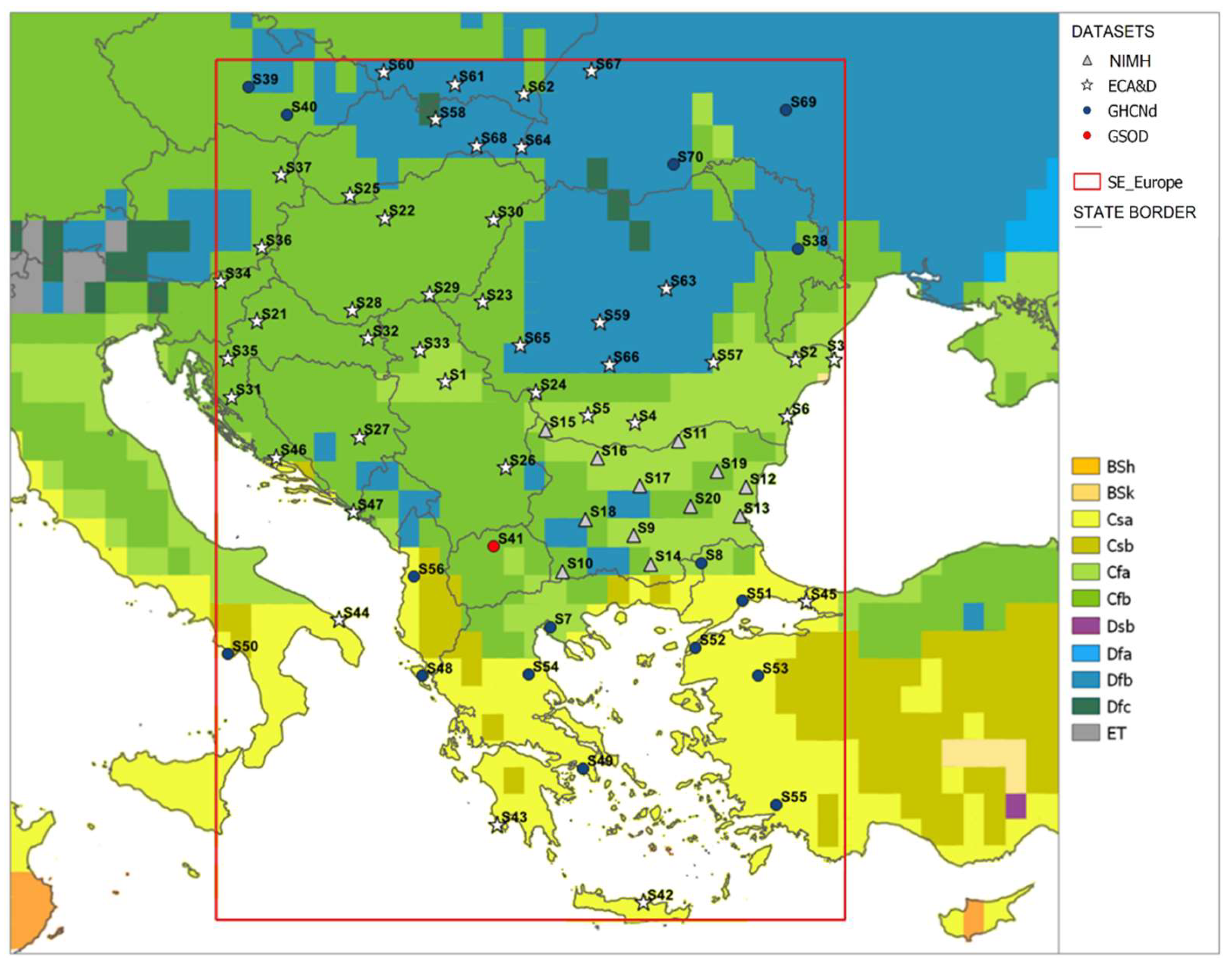
Figure 2.
Left panel: Distribution of calculated empirical quantiles (q2 to q50) on time series of annual minimum temperatures (Tn) for 1961–2020 by stations across SEE; Right panel: Medians (p50); 20th, 15th, 10th, 5th and 1st percentiles (p20, p15, p10, p05 and p01) and absolute minima (min) of daily minimum temperature (tn) for 1961-2020 by climate zones; the range of values used in threshold indicators is shown in bright blue.
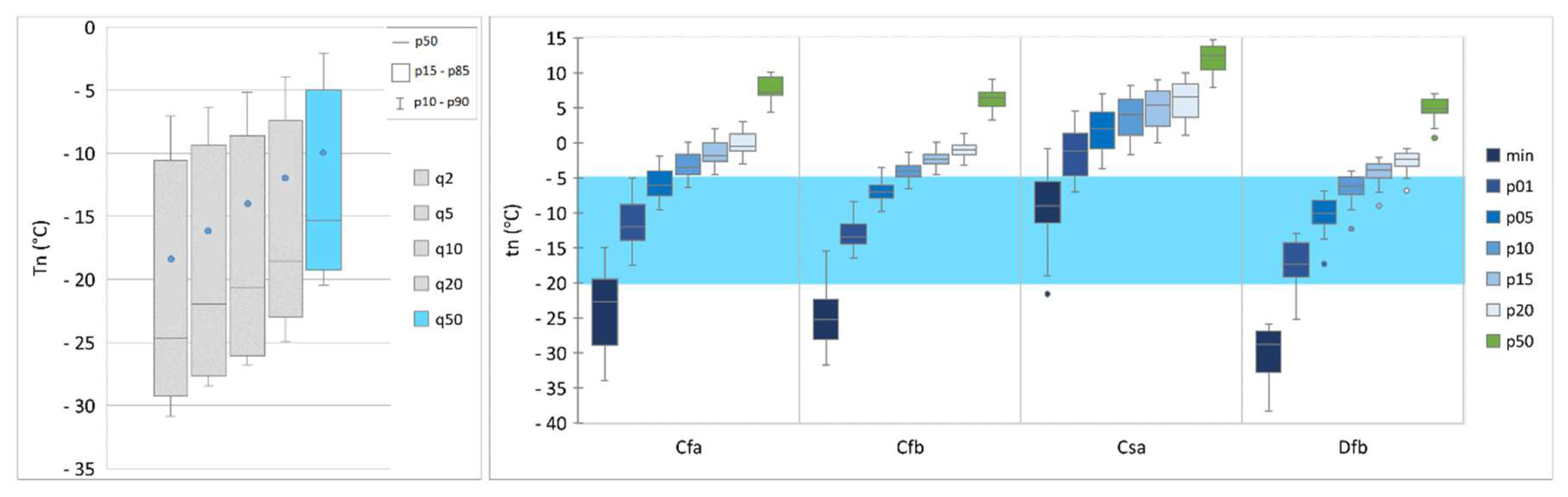
Figure 4.
Long-term variations of ncd-5 and ccd-5 indicators averaged by Köppen-Geiger climate zones.
Figure 4.
Long-term variations of ncd-5 and ccd-5 indicators averaged by Köppen-Geiger climate zones.
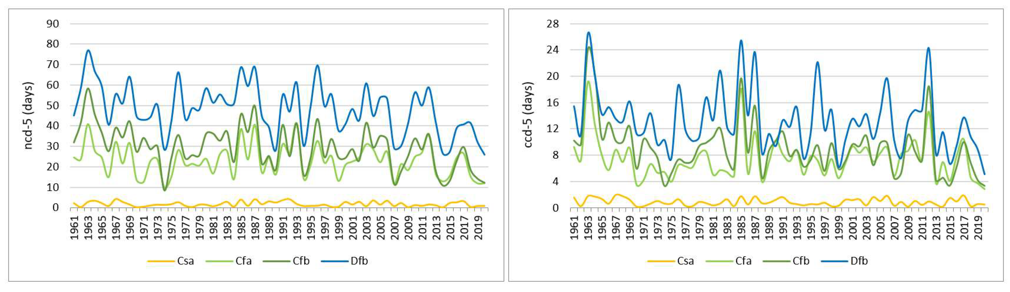
Figure 5.
The multiyear mean of ncd-5 (right panel) and ccd-5 (left panel) indicators for periods 1961-1990 and 1991-2020 and percentage changes relative to 1961-1990 by zones of the Köppen-Geiger climate classification.
Figure 5.
The multiyear mean of ncd-5 (right panel) and ccd-5 (left panel) indicators for periods 1961-1990 and 1991-2020 and percentage changes relative to 1961-1990 by zones of the Köppen-Geiger climate classification.
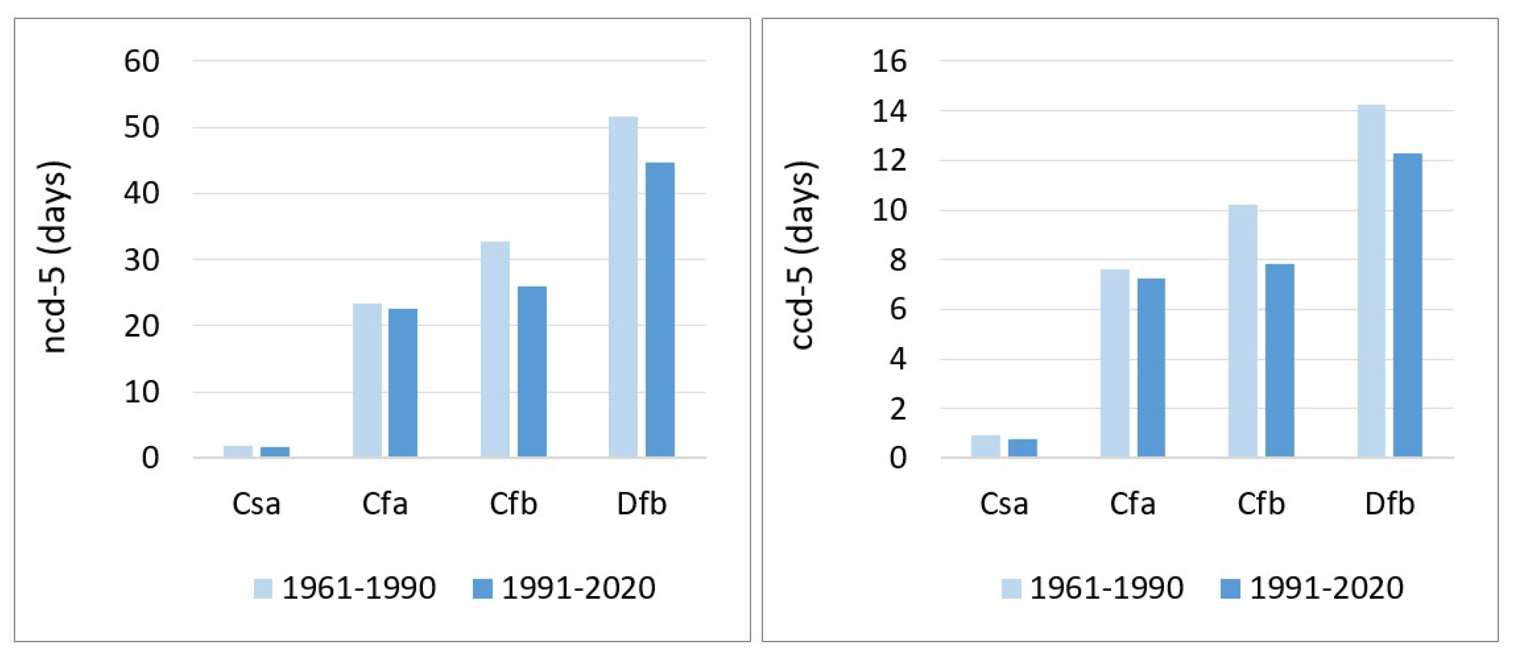
Figure 6.
Long-term variations of csd-5/-10/-12/-14/-16/-18/-20 (unit: days) averaged by Köppen-Geiger climate zones.
Figure 6.
Long-term variations of csd-5/-10/-12/-14/-16/-18/-20 (unit: days) averaged by Köppen-Geiger climate zones.
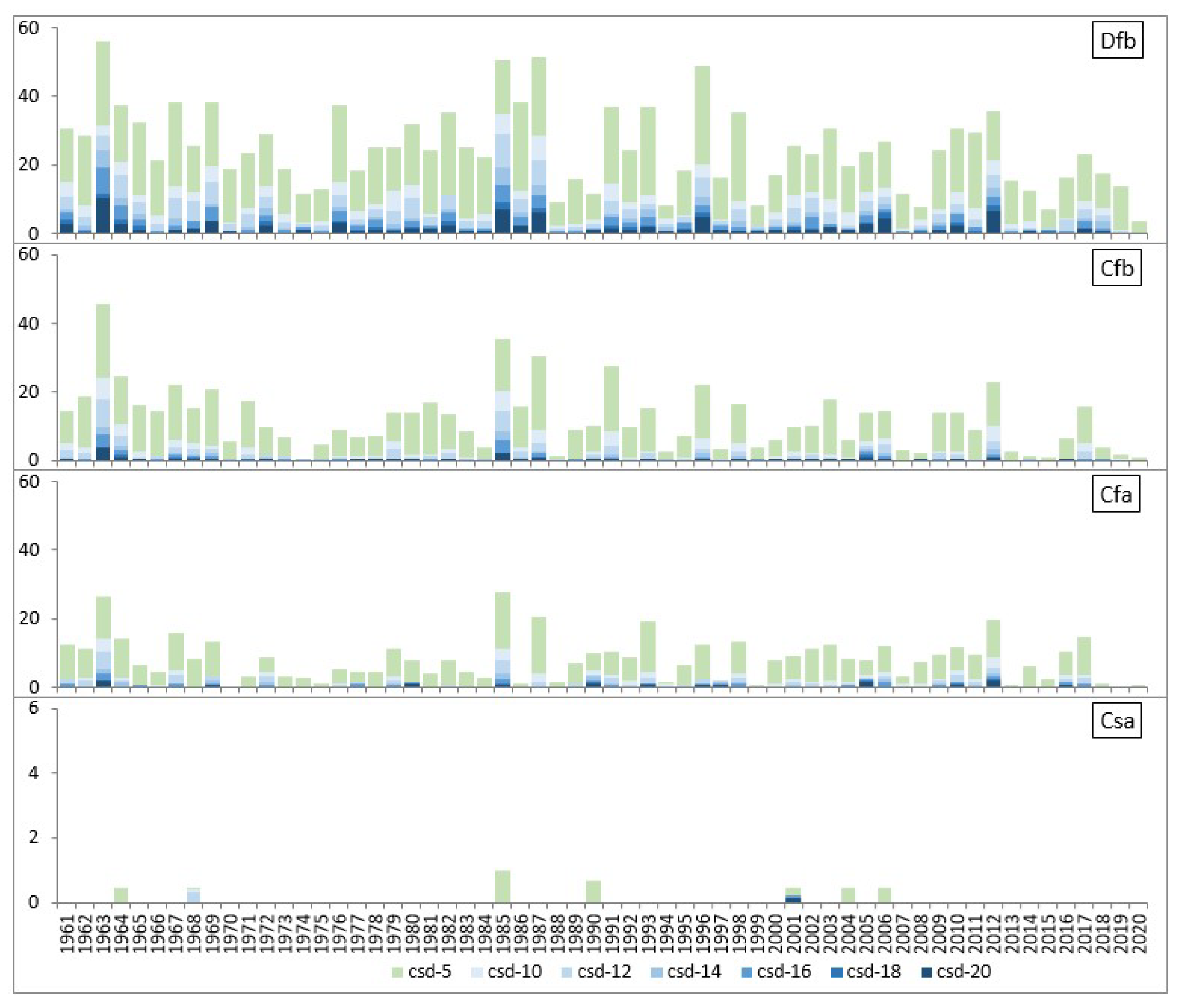
Figure 7.
Long-term variations of ccd-5 and ccd-ECF (unit: days) averaged by Köppen-Geiger climate zones; r denotes the Pearson’s correlation coefficient.
Figure 7.
Long-term variations of ccd-5 and ccd-ECF (unit: days) averaged by Köppen-Geiger climate zones; r denotes the Pearson’s correlation coefficient.
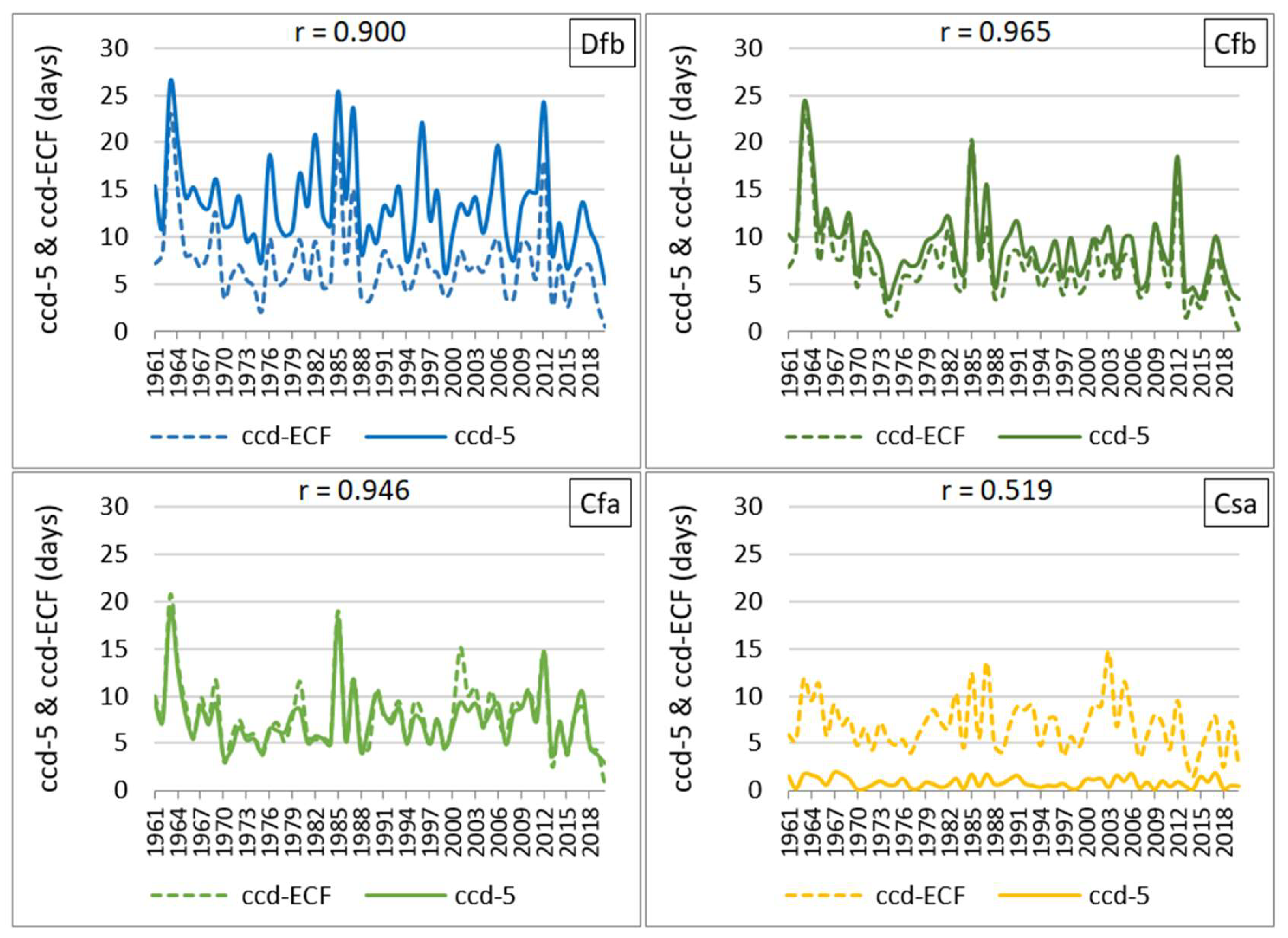
Figure 8.
Scatter-plot of ccd-ECFd vs. ccd-5d. The size of the bubbles is proportional to the yearly maxima of ECFsev calculated by stations and averaged over the SEE domain. Several years by each severity category are shown in different font colors: orange for mild, light blue for severe and dark blue for significantly more severe winters.
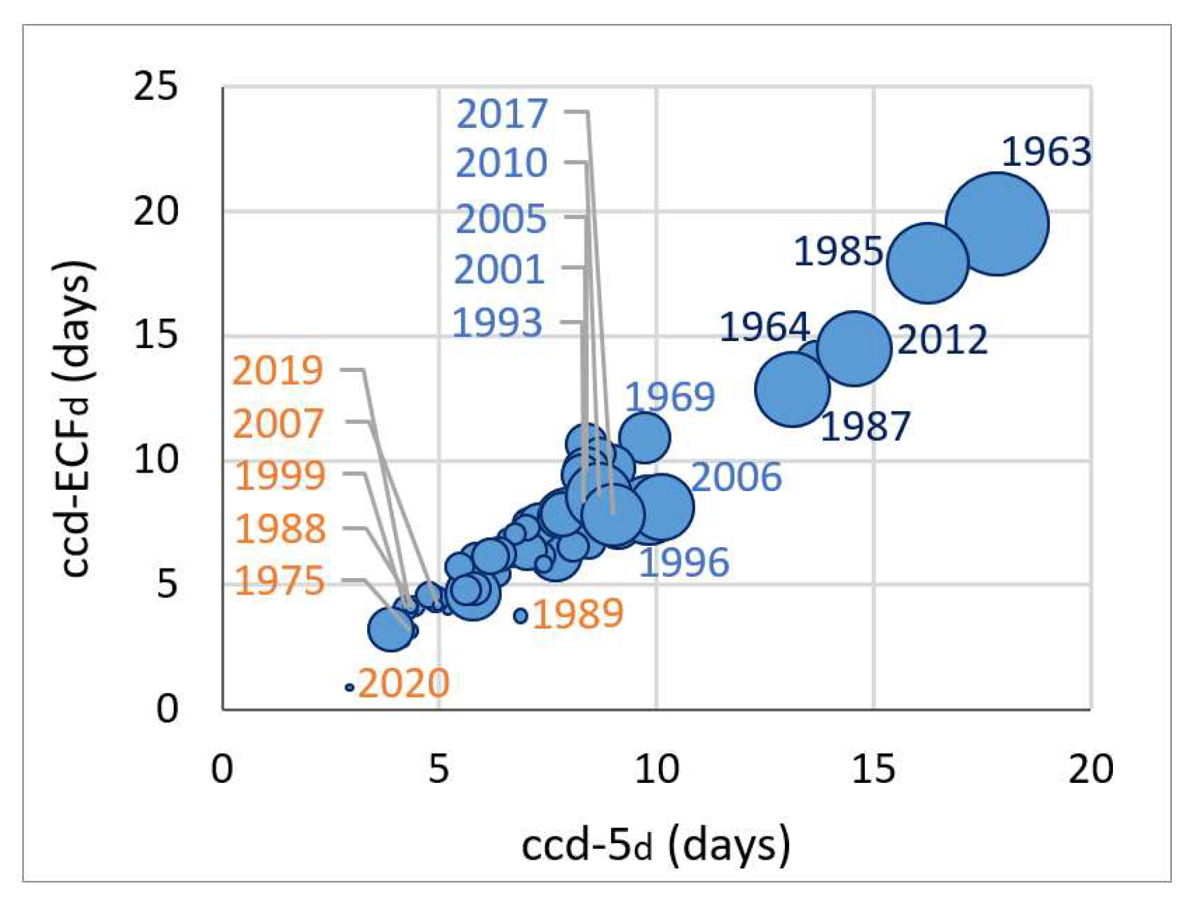
Figure 9.
Left panel: Mean ECFsev across SEE by severity levels according to Nairn et al. [80] for 1961-1990 and 1991-2020 by climate zones; Right panel: Percentage change in the mean ECFsev for 1991-2020; L0 – no excess cold.
Figure 9.
Left panel: Mean ECFsev across SEE by severity levels according to Nairn et al. [80] for 1961-1990 and 1991-2020 by climate zones; Right panel: Percentage change in the mean ECFsev for 1991-2020; L0 – no excess cold.
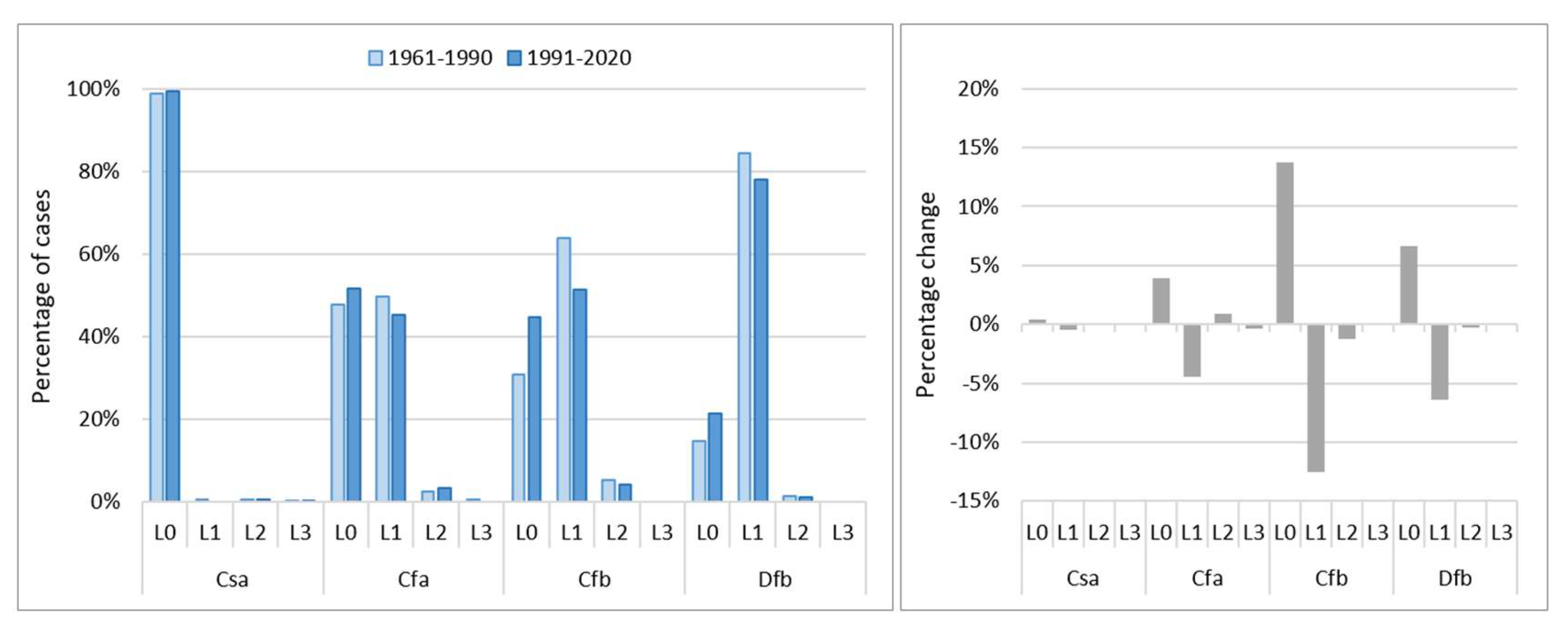
Figure 10.
Left panel: Spatiotemporal variation of yearly maximum ECE intensity represented by categories of csd indicator (bottom) and ECFsev levels (top); Right panel: Percentage of cold spell categories (C1-C7) associated with ECFsev levels (L0-L3). L0 denotes no excess cold.
Figure 10.
Left panel: Spatiotemporal variation of yearly maximum ECE intensity represented by categories of csd indicator (bottom) and ECFsev levels (top); Right panel: Percentage of cold spell categories (C1-C7) associated with ECFsev levels (L0-L3). L0 denotes no excess cold.
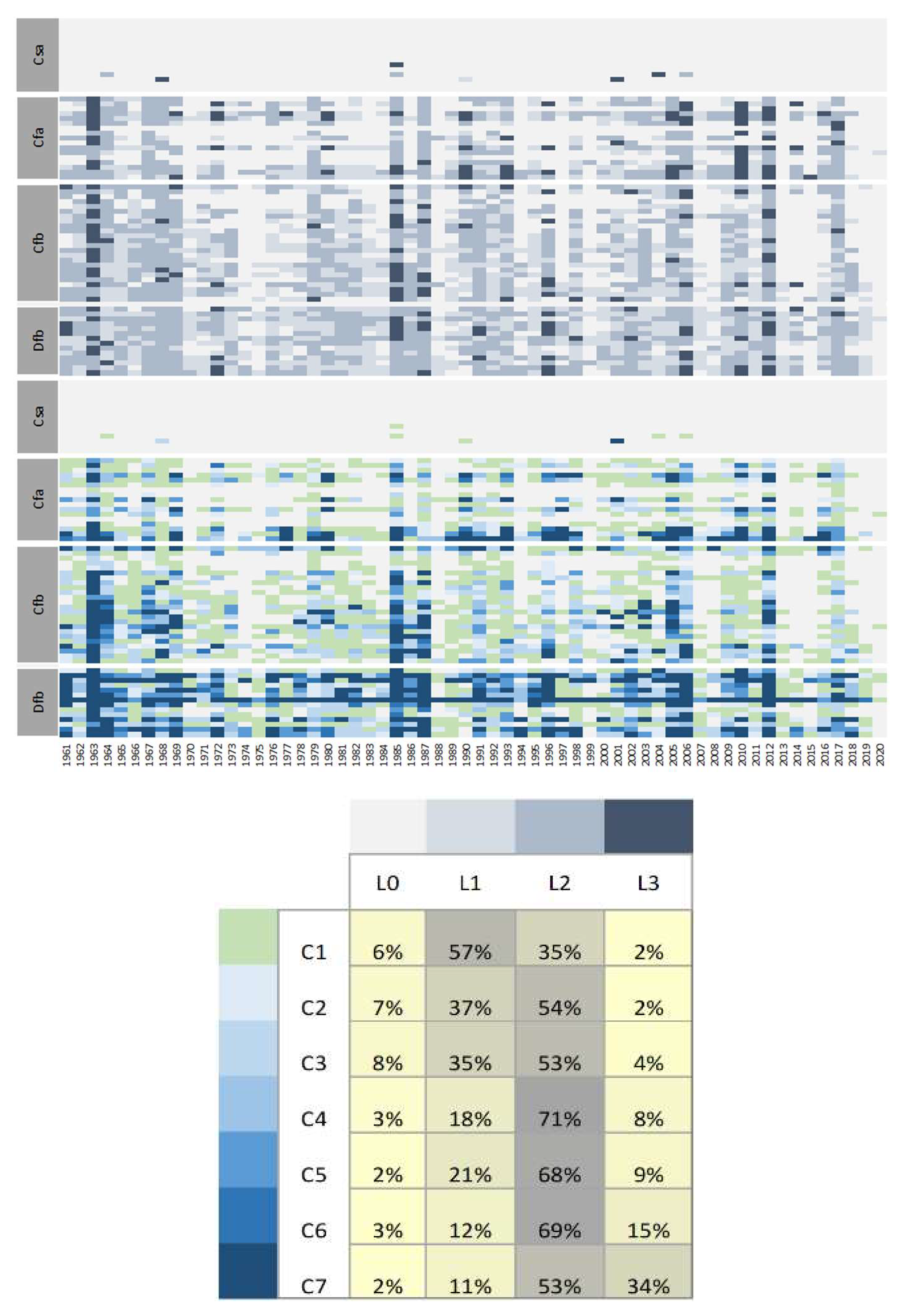
Table 1.
Average/maximum values of Sen’s slope estimates (unit: °C/10 years) of statistically significant linear trends (p < 0.05, Mann-Kendall method) of the annual mean (Ta), annual mean minimum (Tmn) and annual minimum (Tn) temperatures in the period 1961-2020 by zones of the Köppen-Geiger climate classification; IDs of stations (see Appendix A1, Table A1) in which maximum values are reached are shown in brackets; percentage of stations with statistically significant trends is also shown.
| Cfa | Cfb | Csa | Dfb | |||||
|---|---|---|---|---|---|---|---|---|
| Ta | +0.29/ +0.43 (S1) | 100% | +0.39/ +0.55 (S18) | 100% | +0.24/ +0.37 (S45) | 100% | +0.34/ +0.44 (S60) | 100% |
| Tmn | +0.26/ +0.46 (S1) | 82% | +0.34/ +0.58 (S18) | 100% | +0.23/ +0.47 (S45) | 87% | +0.32/ +0.41 (S60) | 93% |
| Tn | +0.54/ +0.54 (S7) | 6% | +0.76/ +1.09 (S37) | 50% | +0.28/ +0.28 (S48) | 7% | +0.79/ +1.00 (S60) | 36% |
Table 2.
Average/maximum values of Sen’s slope estimates (unit: days/10 years) of statistically significant linear trends (p < 0.05, Mann-Kendall method) of threshold indicators in the period 1961-2020 by zones of the Köppen-Geiger climate classification; the values < 0.1 days/10 years are not presented; in brackets are shown stations’ ID (see Appendix A1, Table A1) in which maximum values are reached; percentage of stations with statistically significant trends is also shown.
| Cfa | Cfb | Csa | Dfb | |||||
|---|---|---|---|---|---|---|---|---|
| ncd-5 | -1.5/ -2.3 (S5) | 18% | -3.1/ -4.5 (S34 and S36) | 88% | -3.1/ -4.1 (S60 and S70) | 86% | ||
| ccd-5 | -0.4/ -0.7 (S1) | 18% | -1.0/ -1.3 (S34 and S40) | 67% | -0.8/ -0.9 (S67 and S68) | 43% | ||
| csd-5 | -1.7/ -3.6 (S31 and S39) | 71% | -2.7/ -4.0 (S67) | 79% | ||||
| csd-10 | -0.3/ -0.7 (S34) | 21% | -1.3/ -1.8 (S67 and S69) | 43% | ||||
| csd-12 | -0.8/ -1.6 (S69) | 36% | ||||||
| csd-14 | -0.3/ -0.8 (S69) | 21% | ||||||
| csd-16 | -0.2/ -0.3 (S69) | 14% |
Disclaimer/Publisher’s Note: The statements, opinions and data contained in all publications are solely those of the individual author(s) and contributor(s) and not of MDPI and/or the editor(s). MDPI and/or the editor(s) disclaim responsibility for any injury to people or property resulting from any ideas, methods, instructions or products referred to in the content. |
© 2025 by the authors. Licensee MDPI, Basel, Switzerland. This article is an open access article distributed under the terms and conditions of the Creative Commons Attribution (CC BY) license (http://creativecommons.org/licenses/by/4.0/).
Copyright: This open access article is published under a Creative Commons CC BY 4.0 license, which permit the free download, distribution, and reuse, provided that the author and preprint are cited in any reuse.


