1. Introduction
The India-Eurasia collision and subsequent convergence since last ~55 Ma has produced spectacular topography all along the plate margin (
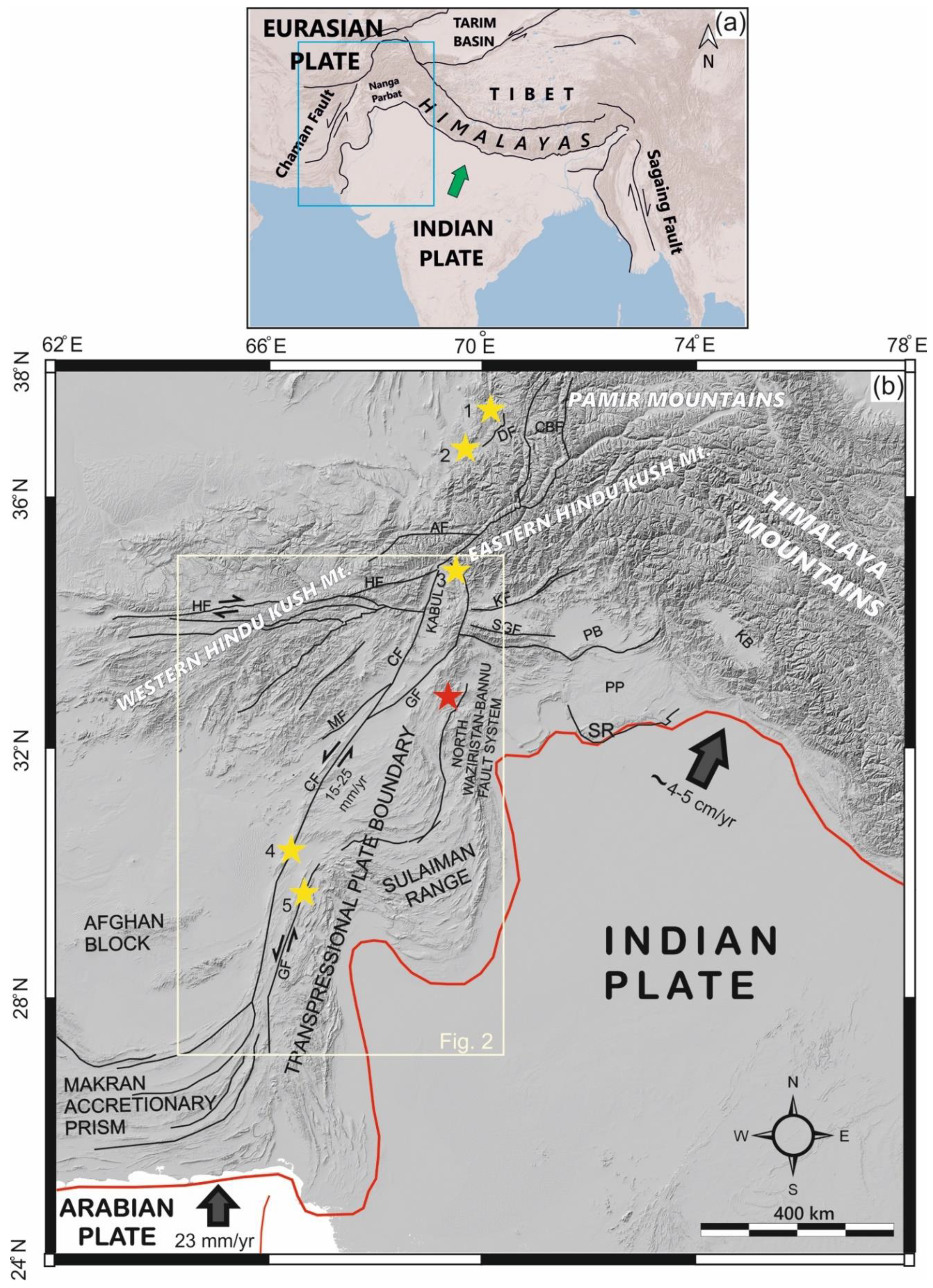
Figure 1). In the north, it is primarily dominated by the thrusting and uplift of the Himalayan mountain belt, whereas along the western and eastern plate boundaries it is controlled by strike-slip faulting along the Chaman Fault (CF) and Sagaing Fault (SF), respectively (
Figure 1). The tectonic boundary all along is characterized by frequent seismicity causing loss of life and property which is a matter of concern to society and scientific community. As a scientific contribution, we present an assessment on the nature of faulting, surface topography and its relationship to the damage caused by the earthquake. In this particular study, the focus is on the western boundary, along which an earthquake occurred on 21 June, 2022 in eastern Afghanistan, close to the border with Pakistan (
Figure 2). The earthquake area is located in a difficult terrain with poor access from either bordering country, where the surface deformation and the reported damages warranted assessment. Because of this, remote sensing techniques play a crucial role in overcoming some of these limitations due to the lack of or limited field observations. Accordingly, InSAR measurements, optical remote sensing observations combined with geological and geomorphic background allowed to elaborate on the co-seismic surface manifestation to constrain the sub-surface geometry of the causative fault segment.
With this premise, we investigated the meizoseismal area of the 21 June, 2022 Afghanistan earthquake to better understand the correlation between long-term deformation signatures in the geology and geomorphology of the area with the short-term remote sensing observations and InSAR measurements along this recently activated fault segment. The causative fault appears to be a part of the broader North Waziristan Bannu Fault system (NWBFS), which extends E-W for more than 100 km (
Figure 1) belonging to the much wider Sulaiman Range.
The major goals of the present note include the: i) mapping of possible cumulative morphotectonic evidence of the reactivated fault segment and its lateral continuity, ii) studying of the InSAR co-seismic deformation pattern of the 21 June, 2022 event, iii) modelling the best-fit fault geometry by inverting the InSAR measurements, and iv) comparison between the long-term and short-term deformation features for obtaining a reasonable fault geometry and its role in seismogenesis.
2. Tectonic Setting
The Materials and Methods should be described with sufficient details to allow others to replicate and build on the published results. Please note that the publication of your manuscript implicates that you must make all materials, data, computer code, and protocols associated with the publication available to readers. Please disclose at the submission stage any restrictions on the availability of materials or information. New methods and protocols should be described in detail while well-established methods can be briefly described and appropriately cited.
The 21 June 2022 earthquake was located close to the western plate boundary of India-Asia convergence (Mallapaty, 2022; Kufner et al., 2023; Roy et al., 2023), where the northward indenting Indian subcontinent moves past the Helmand Block of the Eurasian Plate (Lawrence et al., 1992). As typical in oblique plate convergence settings, deformation is kinematically partitioned (McCaffrey, 1992; Yu et al., 1993; Bowman et al., 2003). Indeed, transcurrency largely occurs along a major lithospheric-scale shear zone referred to as the Chaman Fault System (CFS), while the contractional component perpendicular to the boundary is broadly accommodated within the flysch belt and the Sulaiman Range (
Figure 2). The CFS is a ~1000 km-long, roughly N-S oriented tectonic boundary that extends from the Hindu Kush mountains, in northern Afghanistan, to the Makran coast, in southern Pakistan (e.g. Crupa et al., 2017;
Figure 1). Szeliga et al. (2012) noticed that the current strain rate is further partitioned across the CFS, including the Gazaband and Chaman faults. As a consequence, seismicity is relatively distributed and few earthquakes have been recorded along the Chaman Fault in historical times (Dalaison et al., 2021). This suggests aseismic slip and/or distributed deformation across numerous other structures.
On the other hand, diffuse shortening affects the thick foredeep succession of the Tertiary Katawaz Basin now forming the socalled flysch belt, as well as the sedimentary succession developed along the Mesozoic Indian passive margin. The latter has been largely inverted and mainly detached on top of the underlying transitional-to-oceanic Indian crust thus forming the present-day Sulaiman Range. Overall they describe an active transpressional deformational zone affecting this wide inter-plate setting (
Figure 1). Indeed, the whole system accommodates the ~4-5 cm/yr convergence rate between the Indian and Eurasian plates (Demets et al., 1995; Billham et al., 2001; Banerjee and Burgmann, 2008).
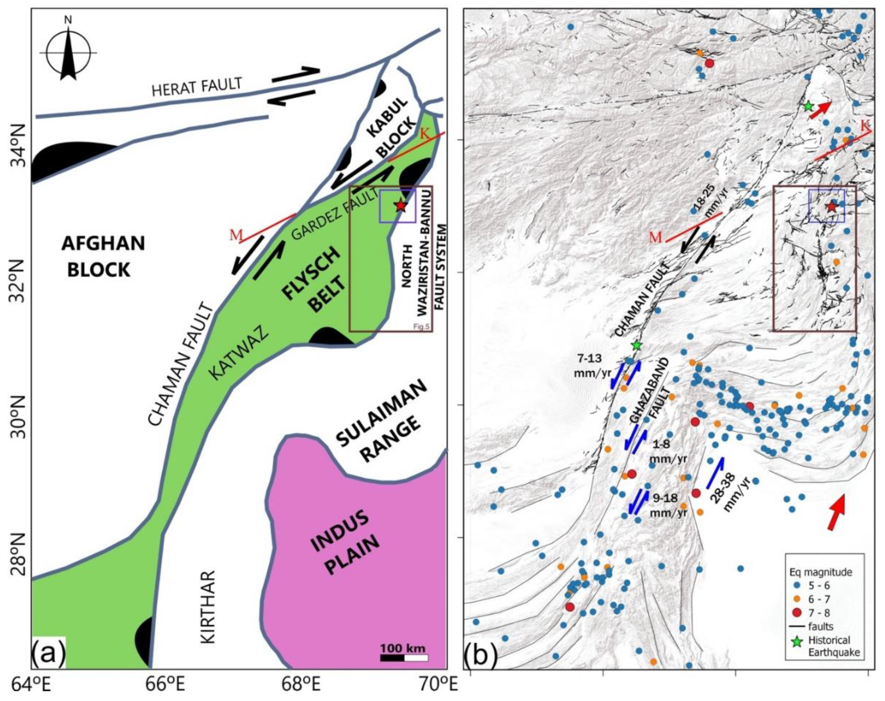
Although the CFS is a relatively sharp geological boundary, there are several synthetic fault splays running sub-parallel to the main structure such as the Gardez Fault (GF), the Mokur Fault (MF), the Konar Fault (KF), etc. (Tapponnier et al., 1981; Ruleman et al., 2007; Shnizai, 2020) forming a broad zone of active deformation. At the boundary between the flysch belt and the Sulaiman Range is the North Waziristan Bannu Fault system: NWBFS (
Figure 2). More precisely, the earthquake of 21 June 2022 occurred on this fault system few kilometres from the eastern border of Afghanistan, where the deposits of the Katawaz Flysch Belt (KFB) are in tectonic contact with the Kurram Group belonging to the south Waziristan accretionary wedge (
Figure 2).
3. Data and Methods
As above mentioned, among the major objectives of the present study is to investigate the long-term and short-term deformation signatures of the new fault segment that caused the earthquake of 21 June 2022 earthquake affecting the region between eastern Afghanistan and western Pakistan. To achieve the objective, published historical and geological maps from various sources and at different scales have been used together with the database of active faults of Afghanistan (Ruleman et al., 2007) and other available works (Shnizai and Walker, 2024 and references therein). The datasets were digitized and stored in a GIS for spatial correlation and analyses. Surface topography data accessed through the United States Geological Survey portal was used to generate shaded relief maps in different perspective directions to highlight topographic features in the attempt of correlating them to known tectonic features. Multi-resolution satellite imageries from Indian Remote Sensing (IRS) satellites and LANDSAT constellation were used to compare observations and inferences represented on geological maps and surface topography. These methods allowed elaborating on the activated fault segment using typical methods of tectonic geomorphology and spatial analyses using satellite remote sensing and digital elevation datasets. Our interpretation of possible recent faulting is based on the presence of prominent and continuous escarpments, strong lineaments in bedrock, linear valleys and typical drainage patterns (Burbank and Anderson, 2009; Duvall and Tucker, 2015; Gill et al., 2021). The data showed good spatial correlation between geologic and geomorphologic features and a comparison with mapped active faults.
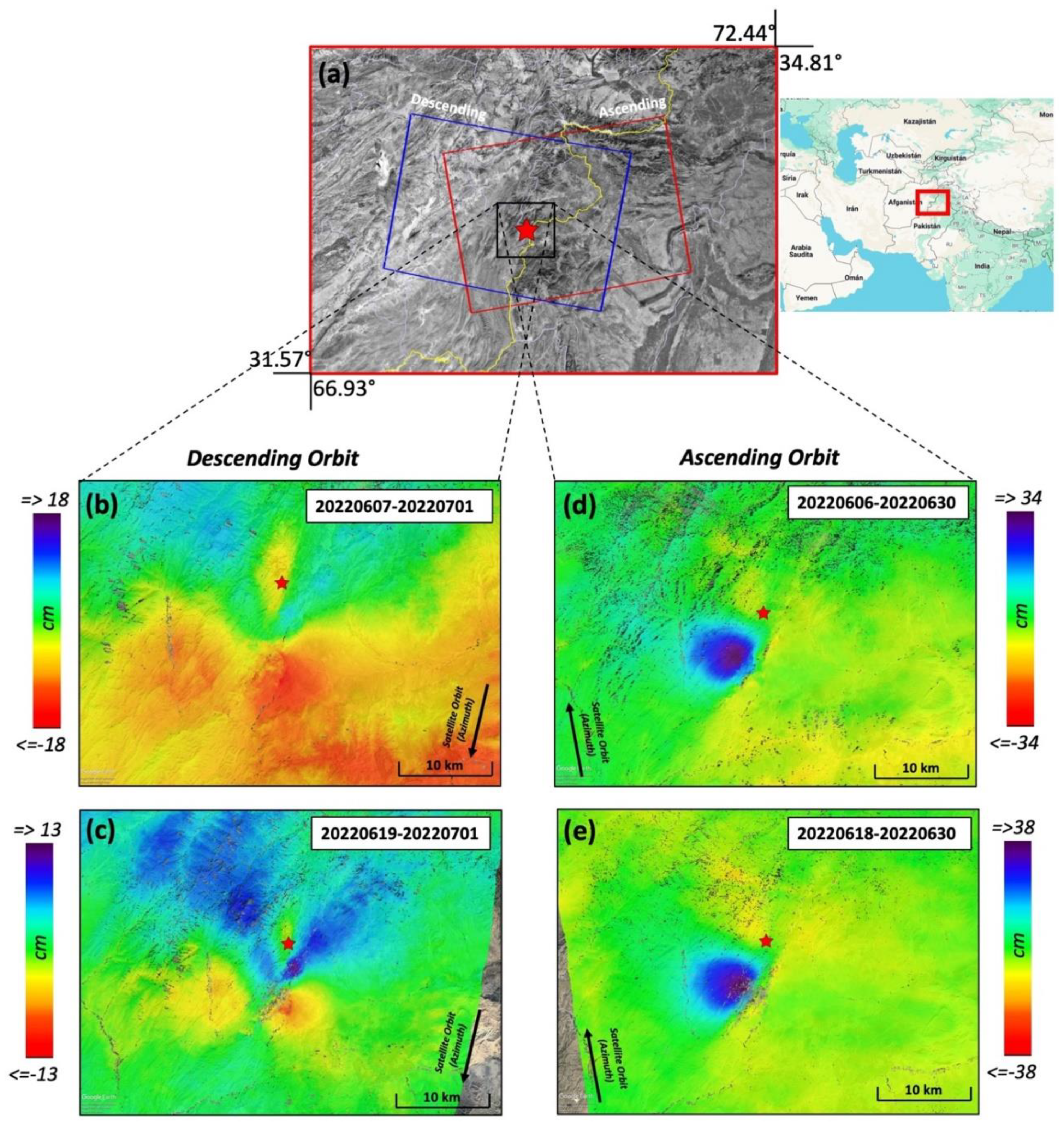
In order to investigate the ground displacement associated to the 21 June 2022 event, we exploited the Differential SAR Interferometry (DInSAR) technique (Massonnet et al., 1993; Burgmann, 2000), which allows the analysis of the surface displacement, by providing a measurement of the ground deformation projection along the radar Line-of-Sight (LoS). The SAR data considered to retrieve the ground deformation associated to the occurred seismic event were acquired by the Sentinel-1 (S1) constellation of the Copernicus European Program, along both the descending (Track 78) and ascending (Track 71). In
Figure 3 we show the location of the earthquake epicentre (identified by a red star), the cover area for both orbits and the co-seismic LOS displacement maps. In
Table 1, instead, we reported several information about the exploited interferometric pairs. In particular, the generated differential interferograms underwent a multilook operation (5 and 20 pixels along the azimuth direction and range, respectively) to finally lead to a ground pixel size of about 73 by 73 m. Subsequently, we generated their corresponding LOS displacement maps through the Minimum Cost Flow phase unwrapping procedure (Costantini, 1998; Costantini and Rosen, 1999). Moreover, for sake of completeness, it is important to highlight that the differential interferograms and the corresponding LOS displacement maps were automatically generated by an unsupervised tool of DInSAR products (Monterroso et al., 2020) and made available on the European Plate Observing System (EPOSAR) service through Thematic Core Service (TCS) of Satellite Data (EPOS 2023).
As described in
Table 1, we benefited from the short revisit time (12 days) and the small spatial/perpendicular baseline separation of the S1 constellation, to generate two interferograms for each orbit by using different primary acquisitions (see
Figure 3). Among them, for the seismic source modelling discussed in the following, we selected those least affected by undesired phase artifacts (e.g. atmospheric phase delays, decorrelation noise), thereby optimizing the reconstruction of the deformation pattern affecting the area (
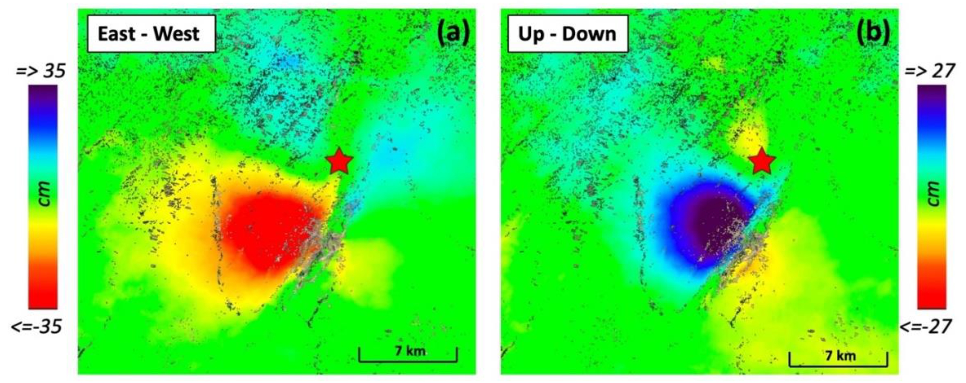
Figure 3a). In particular, the employed S1A data were acquired on 19 June and 01 July 2022, and on 18 June and 30 June 2022 along the descending and ascending orbits respectively. Moreover, by exploiting these displacement maps generated from ascending and descending displacement analysis, was possible to compute the vertical and East-West displacement components (Manzo et al 2006; Casu and Manconi, 2016; De Luca et al 2017). The corresponding results are shown in
Figure 4. More in details, the displacement component maps reveal a maximum deformation of 27 centimeters of uplift and 10 centimeters of subsidence (see
Figure 4b), while the east-west displacement indicates a maximum of 35 centimeters toward to the east and 14 centimeters toward to the west (see
Figure 4a).
The InSAR measurements and fault modelling results (presented in
Table 2) compare well with the already available results (Kufner et al., 2023; Panchal et al., 2023; Qi et al, 2023; Qui et al., 2023; Roy et al., 2023; Dalal et al., 2024). However, there are finer differences which may be mainly due to the differences in down sampling strategies and the boundary conditions input to arrive to the model results.
5. Discussion
Based on the study of geological and geomorphic evidence it appears that the surface manifestation of the active fault responsible for the 21 June 2022 Afghanistan earthquake closely follows the geological boundary between the Katawaz Flysch Basin (KFB) and the Sulaiman Range (SR) towards its northern closure into the North-Waziristan-Bannu Fault system (
Figure 5). In this segment, the fault becomes sub-parallel to the Chaman Fault and is favourably oriented to accommodate a part of the differential motion between the Indian and Eurasian plate. Interestingly, the boundary corresponds to an already identified active fault segment based on landform mapping and geomorphic feature offsets (Ruleman et al., 2007). These observations are also supported by the active fault topographic features elaborated in results section (
Figure 5 and
Figure 6). Based on the data presented here, it is notable that the active fault presents a typical curvature/bend concave towards west which encloses a sharp topographic ridge on its western side. Due to the earthquake, landslides were clustered all around the ridge (Shnizai et al., 2022). It is noticeable that the fault curvature/bend is an offset from the main fault and corresponds well to the width of the ridge. The ridge becomes wider in the south-central part and swiftly narrows down towards its northern termination forming an en-echelon pattern of ridges (
Figure 7). Such en-echelon patterns are typical of fault step-overs (Wang et al., 2017). In this particular case, the step-overs formed restraining bends thus generating push-up ridges. It is well known that the strong compression near the inside corners of these restraining bends cause increased uplift rates forming sharp ridges (Cowgill et al., 2004; Garvue et al., 2023). The spatial correspondence of all the above manifestations suggests a strong connection between the seismogenic fault and surface topography (
Figure 6 and 7).
At the same time, the co-seismic interferograms show a perfect linear fault trace, with clear lobes of different LOS displacements (
Figure 8). Although the InSAR fault trace is slightly offset (~1-2 km westwards) relative to the morphotectonic evidence, the two have almost the same average strike and correspond well with the length of the sharp topographic ridge (
Figure 5 and
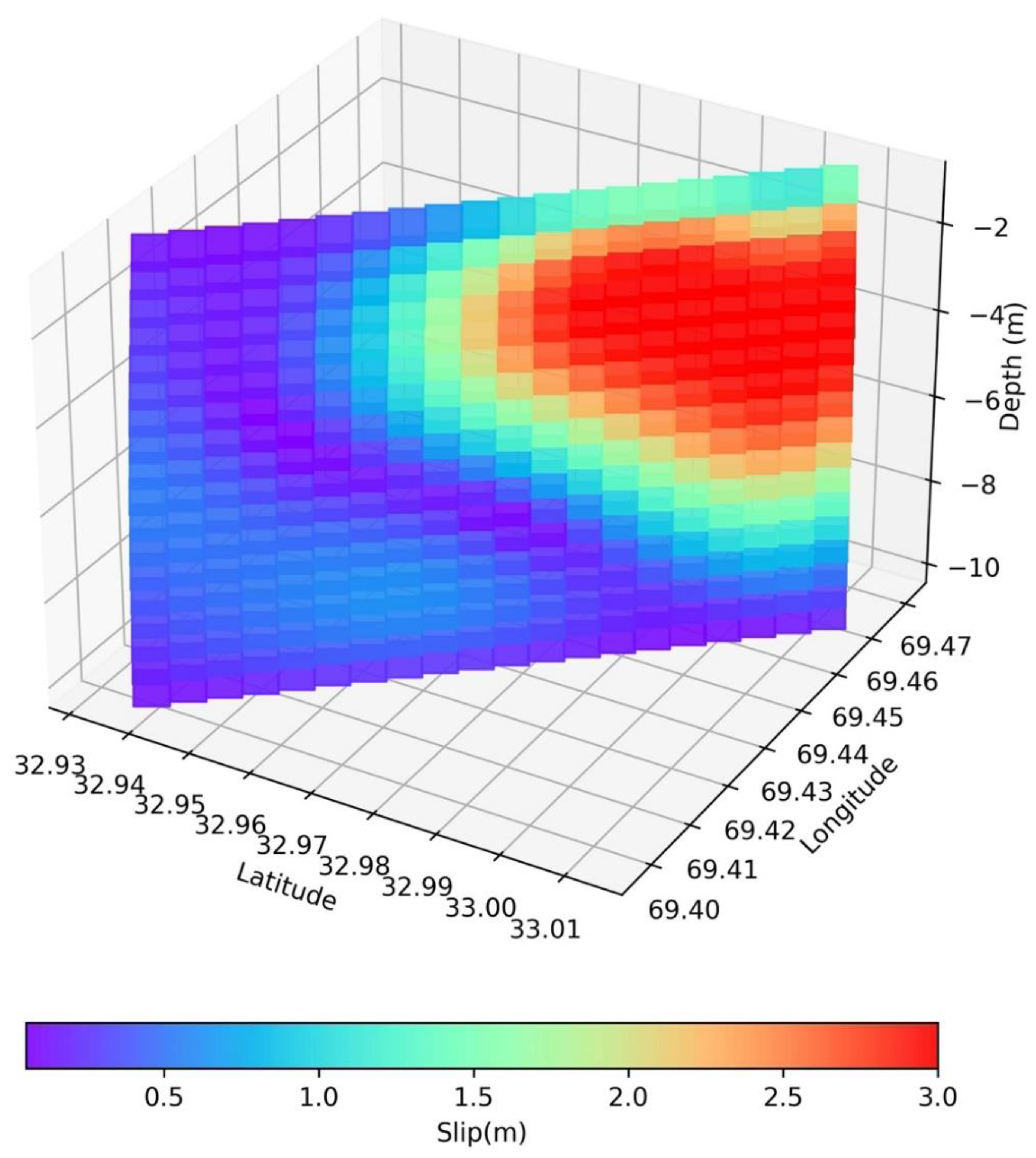
Figure 6). Following the slip model the fault terminates upwards at a shallow depth of about 1 km and it does not reach the surface (
Figure 9). Considering this information, it is seen that the InSAR LOS displacements and topographic profiles show the corresponding maxima towards the south-central part of the ridge, where the ridge attains its maximum width and elevation (
Figure 5 and
Figure 6). The LOS-displacements tend to reduce northwards along the fault line and appear to follow the narrowing topography of the ridge (
Figure 7 and
Figure 10). A similar observation has been reported based on the coherence maps which suggest a wider damage zone in the south-central part (Kufner et al., 2023).
The previous arguments suggest that the active fault derived from the morphotectonic analysis is slightly offset from the one derived on the basis of the co-seismic LOS displacements (
Figure 10). This may be primarily due to two reasons: i) InSAR was unable to capture the deformation geometry in the area closer to the surface fault. This could be due to loss of coherence caused by the severe shaking and the randomly distributed surface deformation, as also seen by severe landsliding along the ridge crest. ii) The fault geometry changed near to the surface as the fault model is unable to capture any surface rupture. In the shallow sub-surface the faults commonly tend to either follow local geological discontinuities or any other inherited weakness zone.
Further, based on the very few ground reports (Kufner et al., 2023), a series of secondary features such as landslides, building damage, fractures, syn- and antithetic Riedel shears have been observed in the field. However, no reports of any primary surface rupture is available, similar to the fault modelling results (
Table 3). As most of these sites are at least 1.5 km west of the InSAR fault trace, they do not offer any direct insights into the fault setting and geometry. Moreover, InSAR results and model calculation suffer from the coherence loss in the area related to fault line. Therefore, it could be reasonably assumed that the InSAR technique is able to capture the general geometry of the fault at depth where it is continuous and relatively smooth. However, it is unable to capture it at close range and shallow depth. This is where a morphotectonic approach becomes important and any deviation between the two fault traces may arise due to geological complexities and/or InSAR method limitations. Indeed, based on our own analyses and fault model, it is likely that no primary surface rupture has occurred during this earthquake. This major conclusion and a similar fault geometry and kinematics, i.e. subvertical fault surface with sinistral slip (Shnizai et al., 2022; Kufner et al., 2023; Roy et al., 2023, this study), could be reasonably reached based on the secondary field evidence and modelling results. It is also important that as the fault does not rupture to the surface the deformation patterns have to be judiciously interpreted using secondary effects which are commonly controlled by the local geological conditions.
Interestingly, the field observations are limited within the western part of the InSAR fault trace and there is no real ground information from the eastern sector near to the active fault trace of Ruleman et al. (2007). This leaves an interpretative uncertainty that could be solved by combining the geologic/geomorphic observations with the InSAR measurements (
Figure 8 and
Figure 10). It is revealed that the geologic/geomorphic active fault is located ~1-2 km east of the InSAR fault trace (
Figure 10), where there is a cluster of landslides on the ridge (Shnizai et al., 2022) corresponding to the area of coherence loss (Kufneer et al., 2023; this study). Although the InSAR fault trace corresponds to the maximum change in LoS displacements on either side surrounded by a pronounced zone of coherence loss, there is absence of any corresponding discernible topographic manifestation (
Figure 6,
Figure 7 and
Figure 10). Conversely, the active fault trace of Ruleman et al. (2007) bears the most discernible active fault features: i) fresh cluster of landslides on the ridge and ii) bends in the ridge typical of left-lateral kinematics. Most importantly, these two ridge anomalies correspond to the continuous zone of coherence loss along the ridge (
Figure 8).
Accordingly, it is inferred that the InSAR fault trace is slightly offset from the morphotectonic feature, it may represent two aspects of the same fault. The InSAR based fault model represents the broader sub-surface geometry of the fault plane matching the Co-Seismic LOS deformation pattern (
Figure 10 and
Figure 11). This fault-plane is blind and do not actually rupture the surface. On the contrary, the observed morphotectonic feature represents the shallow evidence of the same structure that could slightly deviate from the broader sub-surface geometry due to the fact that the confining pressure decreases upwards and repeated ruptures could occur along more variable paths. This could allow the fault to deviate from an ideally flat geometry and instead follow local geological heterogeneities, like layering, or structural discontinuities. In case of transcurrent faulting, similar local variations commonly give rise to releasing or restraining bends (Cowgill et al., 2004; Ye et al., 2015; Gabrielsen et al., 2023; Garvue et al., 2023). At this regard, the deviation between the InSAR and geologic/geomorphic fault traces for the investigated case corresponds with such a bend along the strike, where the geometry of the fault suggests the occurrence of a right stepping left-lateral structure which is expected to produce local uplift with the formation of a pop-up ridge within the restraining bend (
Figure 6 and
Figure 7). Towards the north, the restraining bend disappears along the fault trace, thereby confining the ridge which is wider in the southern and central part and narrows down northwards (
Figure 6 and
Figure 7). Such subtle but possible correlation between the topographic features and the bend along fault strike might have been missed by the InSAR technique mainly due to the local coherence loss, the geometry of imaging and/or the blind nature of the fault.
In summary, it is proposed that in the shallow sub-surface i.e. up to ~ 1-2 km the fault plane is sub-vertical due to large confining pressures from the adjoining fault blocks. However, the situation changes significantly in the near surface where the reduced overburden and confining pressure is considerably reduced. The fault is unable to maintain itself into the same plane, rather it takes preferential paths along pre-existing geological discontinuities such as the rock foliation that coincide with the fault strike as reported from sites recorded by Kufner et al. (2022), but with gentler dips (~ 30° - 60°) westward. Such a change/bend in fault strike forms a geometrical complexity making a restraining bend which is manifested by the topographic ridge. The restraining bend acts as a subtle barrier that can effectively hinder slip on the fault plane causing high strain zones (Cowgill et al., 2004; Wang et al., 2024). Model results also show increased deviatoric stress and high strain rates around fault stepovers and restraining bends (Wang et al., 2017). Fault stepovers localize strain and they have been identified as loci of both initiation and termination for seismic ruptures (King and Nabelek, 1985). This suggests that such step-overs play an important role in controlling the size and extent of earthquakes and consequently the seismic hazard around strike-slip fault zones (Avouac et al., 2014; Wang et al., 2017; 2024).
Figure 1.
The India-Asia convergence zone a) showing the major thrusts towards the north generating the Himalayan mountain belt and the western and eastern boundary showing the major strike-slip faulting along the Chaman Fault (CF) and Sagaing Fault (SF), respectively. b) The western plate boundary defined by the localized deformation along the Chaman Fault (CF) and a series of subsidiary faults trending parallel to sub-parallel to it spread out over a wide lithospheric shear zone forming the Chaman Transpressional Zone (CTZ). The yellow stars show major historical earthquakes along the CTZ and the red star the 21 June 2022 event.
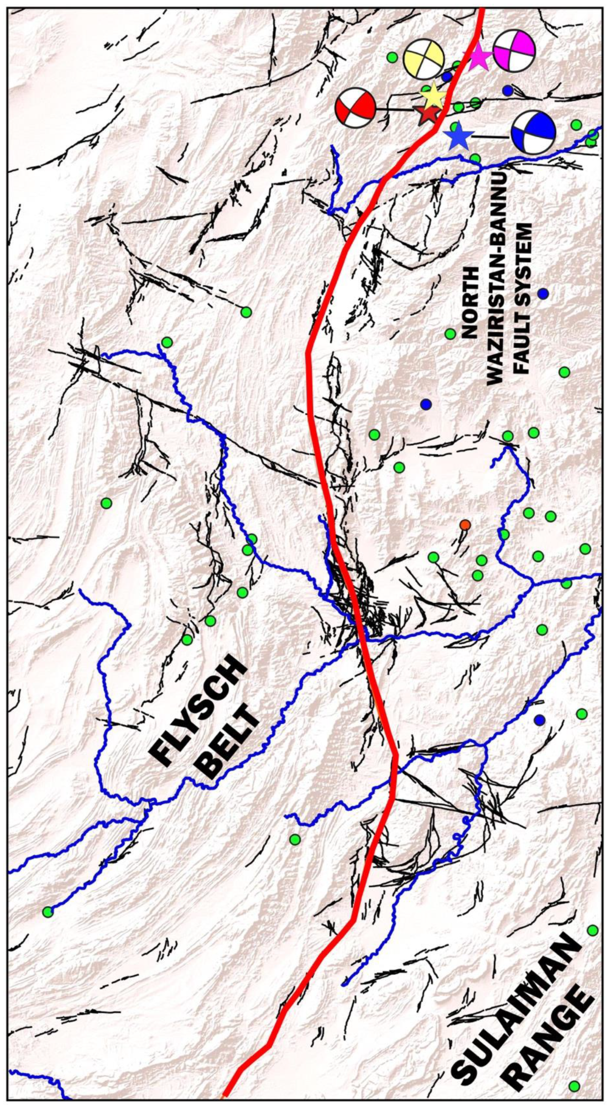
Figure 2.
a) Tectonic divisions of the Western Plate boundary showing major faults by bold lines and subsidiary structures by normal lines. b) Active Faults from Ruleman et al. (2007) and seismicity > 5 (USGS), bold arrows shown tectonic transport direction. M: Mokur Fault and K: Konar Fault. Black filled spaces represent ophiolites.
Figure 3.
Sentinel-1A coseismic LOS displacement results relevant to the 21 June 2022 earthquake of Eastern Afghanistan. (a) indicates the Sentinel-1A footprints used to cover the area of interest (Ascending orbit red line and Descending orbit blue line). (b) and (c) show the coseismic LoS displacement maps for the descending orbit. (d) and (e) show coseismic LOS displacement maps for the ascending orbit.
Figure 4.
Horizontal (East-West) and Vertical (Up – Down) displacement component of coseismic results relevant to the 21 June 2022 earthquake of Eastern Afghanistan. (a) East – West and (b) Up – Down coseismic displacement maps, respectively.
Figure 4.
Horizontal (East-West) and Vertical (Up – Down) displacement component of coseismic results relevant to the 21 June 2022 earthquake of Eastern Afghanistan. (a) East – West and (b) Up – Down coseismic displacement maps, respectively.
Figure 5.
Red line shows that general trace of the fault separating the flysch belt of the Katawaz Basin in the west, which forms the NWBFS towards the north, from the Sulaiman Range in the east. The 21 June, 2022 event is shown by star symbol. Stars represent epicentres with focal mechanisms from different agencies: Yellow (USGS), Pink (GFZ), Blue (GCMT) and Red (this study). Black lines are active fault segments from Ruleman et al. (2007). Dots represent minor seismicity. For location refer Fig. 2. (Add larger drainage offsets along the red fault and different colour of beach balls).
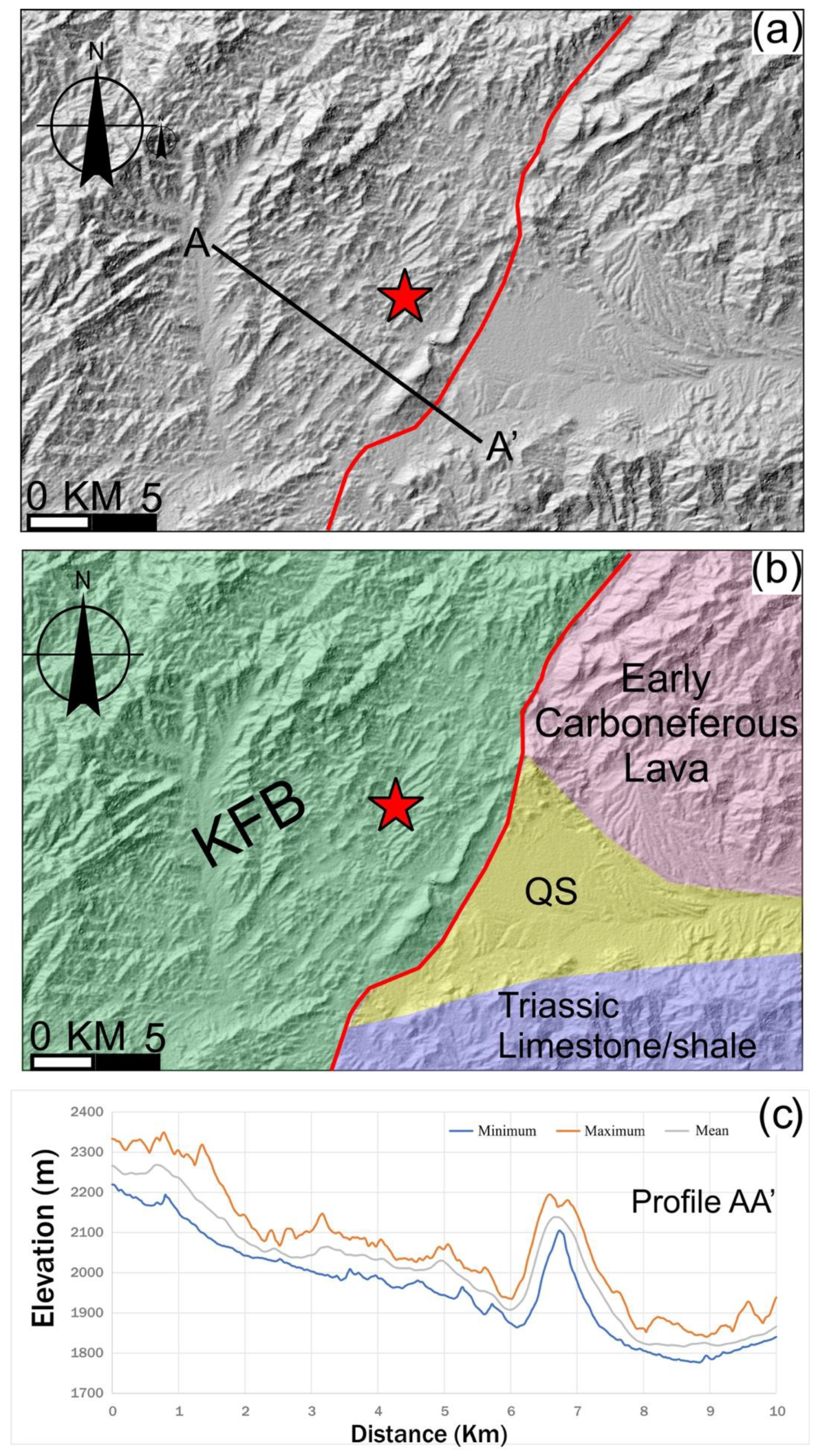
Figure 6.
Generalized setting of the epicentral region of the 21 June, 2022 earthquake (marked by the red star). The red line conforms to the trace of the active fault a) DEM highlighting the abruprt rise of the ridge along the bend of the fault. b) geological map showing the ridge directly abutting against the Quaternary Sediment (QS). c) Swath profiles display the abrupt rise of the ridge in comparison to the surrpounding topography. Profile line is A-A’.
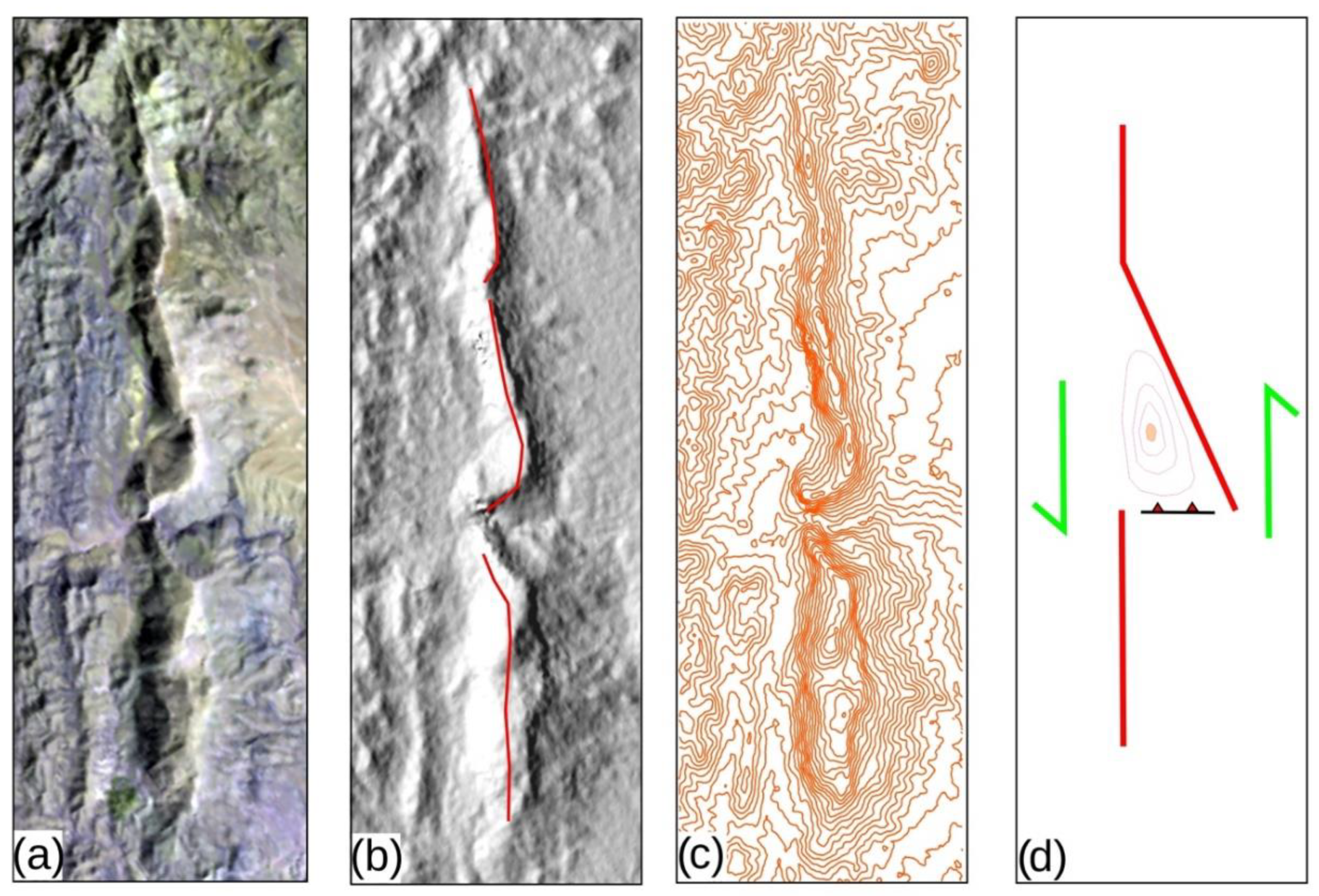
Figure 7.
The arrangement of right stepping fault bends forming a segmented ridge topography in a left-lateral environment. a) as seen on Satellite Image b) as seen in DEM, the red lines follow the ridge top c) contours for better visualization and d) Schematic model showing evolution of the observed fault bend and related ridge topography across the fault step-overs. The contours inside the bend show the ridge topography (high in the centre).
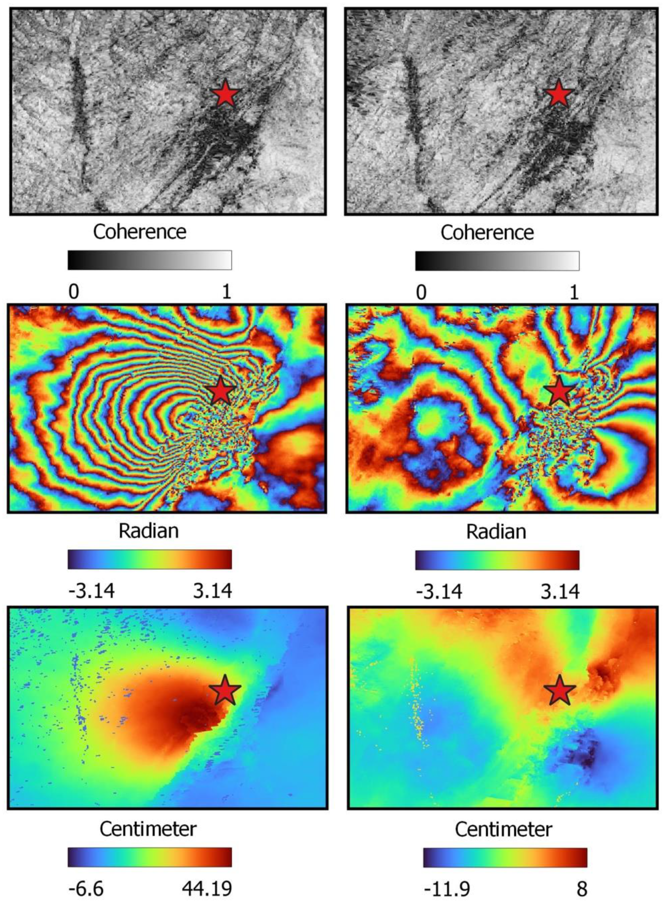
Figure 8.
InSAR results for the 21 June, 2022 earthquake, USGS epicentre shown by the red star. Results from the Ascending mode (left panel) and Descending mode (right panel). Coherence maps (top panel), phase change fringes (middle panel) and LOS displacement (bottom panel).
Figure 8.
InSAR results for the 21 June, 2022 earthquake, USGS epicentre shown by the red star. Results from the Ascending mode (left panel) and Descending mode (right panel). Coherence maps (top panel), phase change fringes (middle panel) and LOS displacement (bottom panel).
Figure 9.
The 21 June, 2022 Afghanistan earthquake fault model showing variable slip distribution along the fault plane.
Figure 9.
The 21 June, 2022 Afghanistan earthquake fault model showing variable slip distribution along the fault plane.
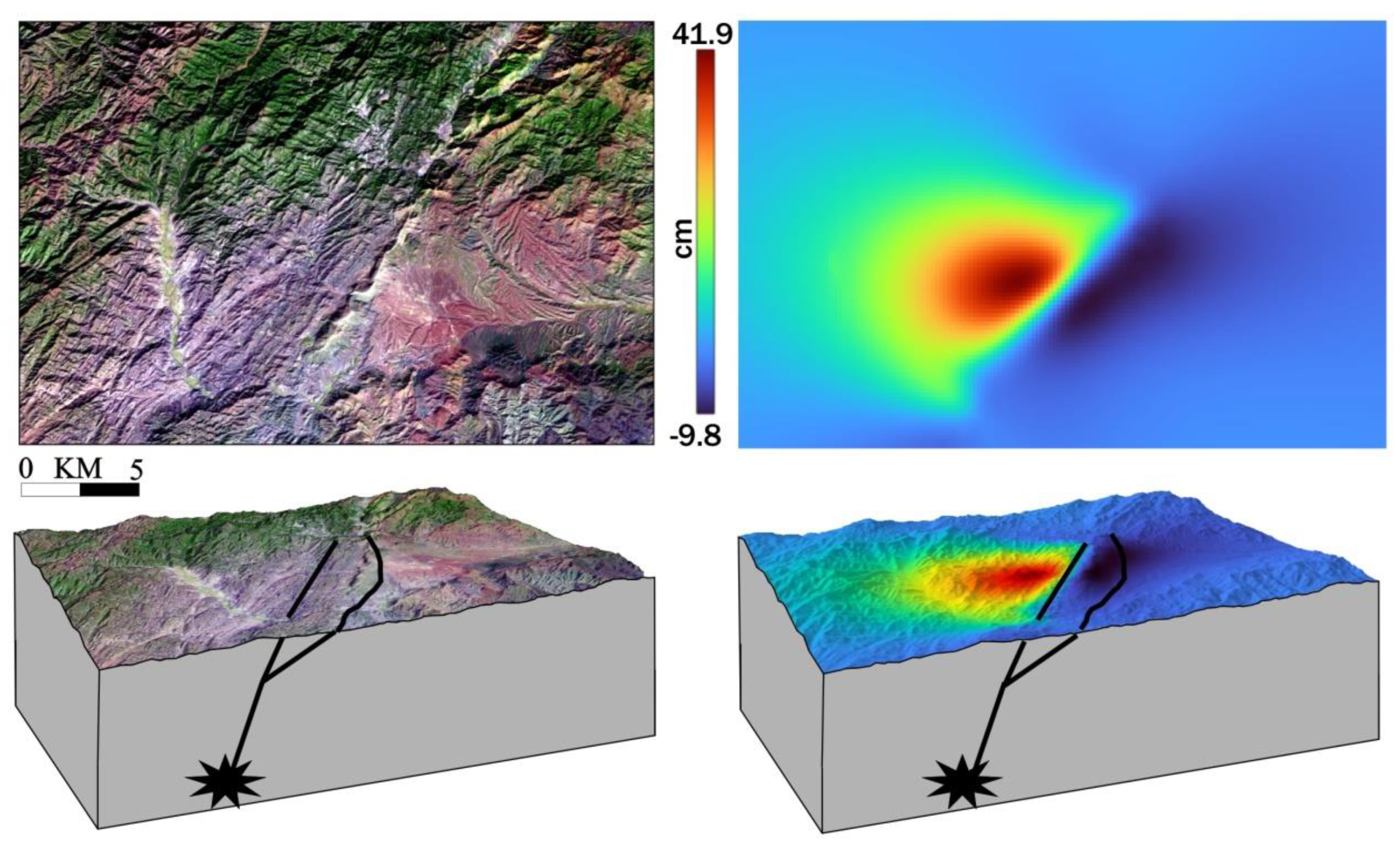
Figure 10.
The top panel shows the active fault derived from a) surface topography and b) Co-seismic LOS displacements. The lower panel shows the respective 3-D perspective views of the active fault derived from a) surface topography and b) Co-seismic LOS displacements. The star shows the focus of the earthquake and black bold lines in section view are sub-surface reconstructions of the active faults.
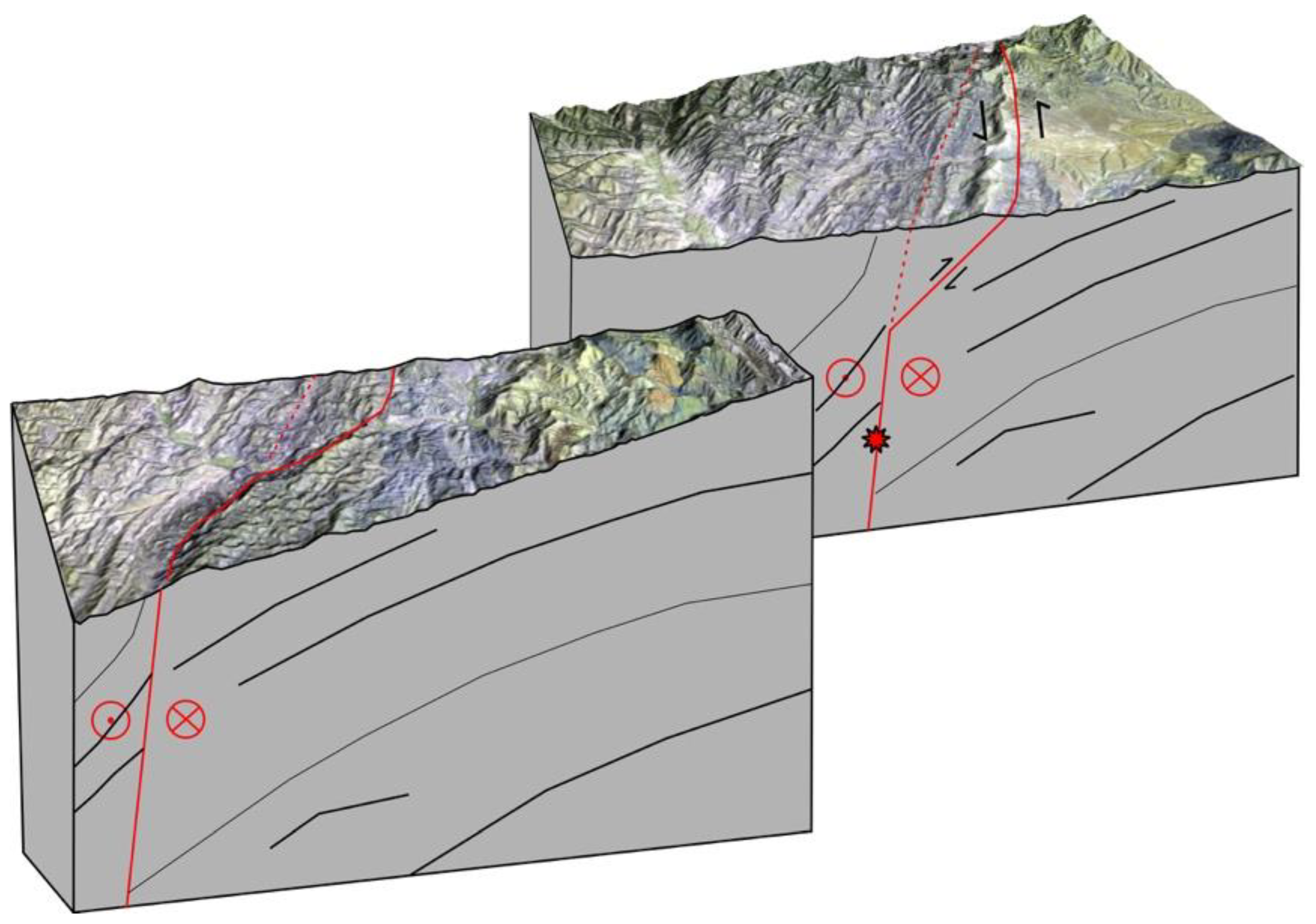
Figure 11.
A schematic 3D perspective of the fault geometry. The two blocks contain the same fault line but have been offset only to help better visualization of the fault geometry in the sub-surface and near-surface The offset of blocks does not represent the movement along the fault. The actual fault geometry inferred from this study is shown as a continuous red line in the section view, that deviates from the the InSAR faultline (shown as dashed red line).
Table 1.
Main characteristics of the interferometric pairs considered for the seismic source modelling of the Mw 6.0 earthquake at southwest of Khost, Afghanistan.
Table 1.
Main characteristics of the interferometric pairs considered for the seismic source modelling of the Mw 6.0 earthquake at southwest of Khost, Afghanistan.
| Sensor |
Primary-Secondary |
Orbit |
Track |
Perpendicular Baseline [m] |
| Sentinel-1A |
2022.06.06-2022.06.30
2022.06.18-2022.06.30 |
Ascending |
71 |
-15.1934
-165.464 |
2022.06.19-2022.07.01
2022.06.07-2022.07.01 |
Descending |
78 |
-76.3265
-7.78262 |
Table 2.
Existing fault model results from previous studies compared to this study.
Table 2.
Existing fault model results from previous studies compared to this study.
| PARAMETERS |
USGS |
GCMT |
GFZ |
IPGP |
Panchal et al. (2023) |
Qi et al. (2023) |
Roy et al. (2023) |
Kufner et al. (2023) |
THIS STUDY |
| EPICENTRE |
33.02°N 69.46°E |
32.94°N 69.51°E |
33.10°N 69.5°E |
33.11°N 69.53°E |
- |
69.46˚°N 32.99°E |
- |
33.0°N 69.5°E |
33.01°N 69.46°E |
MAGNITUDE
(Mw)
|
6.02 |
6.2 |
6.1 |
6.2 |
5.99 |
6.32 |
6.18 |
6.18 |
6.2 |
| STRIKE |
204° |
202° |
104° |
220° |
218° |
203.7° |
216° |
212.75° |
214.41° |
| DIP |
87° |
57° |
89° |
70° |
72.8° |
68° |
61.9° |
72.04° |
80° |
| RAKE |
-11° |
10° |
165° |
-3° |
- |
6.9° |
- |
14.08° |
24.9° |
| DEPTH (Km) |
11.5 |
15.5 |
10 |
6 |
7.1 |
2.5 |
- |
4.92 |
3.56 |
| SLIP (m) |
0-1.5 |
- |
- |
- |
1.05 |
0-3 |
0-2.26 |
1.91 |
0-3 |
| LENGTH (Km) |
- |
- |
- |
- |
7.5 |
20 |
- |
5.91 |
10.33 |
| WIDTH (Km) |
- |
- |
- |
- |
6.0 |
12 |
- |
- |
9 |
Table 3.
The model parameters for ascending, descending and joint inversion (data to be added).
Table 3.
The model parameters for ascending, descending and joint inversion (data to be added).
| Latitude (Degree) |
33.01 |
| Longitude (Degree) |
69.46 |
| Magnitude |
6.2 |
| Depth (Km) |
3.56 |
| Length (Km) |
10.33 |
| Width (Km) |
9 |
| Strike (Degree) |
214.41 |
| Dip (Degree) |
80 |
| Mean Slip (Meter) |
1.08 |
| Max Slip (Meter) |
3 |
| Rake (Degree) |
25 |
| Data-Model Correlation |
0.87 |