
Submitted:
04 February 2025
Posted:
05 February 2025
You are already at the latest version
Abstract
The city of Aïn Témouchent, located in northwest Algeria at the westernmost part of the Lower-Cheliff Basin, has experienced several moderate earthquakes in the past. The most significant event occurred on December 22, 1999, with a magnitude of Mw 5.7, resulting in 25 fatalities and severe damage to the town center. In this study, ambient noise measurements from 62 sites have been analyzed using the horizontal-to-vertical spectral ratio (HVSR) method to estimate the fundamental ground frequencies (f₀) and their corresponding amplitudes (A₀). The results reveal that f₀ varies between 0.8 and 4.8 Hz, with amplitudes ranging from 2 to 5.6. The inversion of the HVSR curves enabled the estimation of the sedimentary layer profiles, with the corresponding thickness variation and shear–wave velocity for each layer. Additionally, four array measurement points across the city center were carried out using the spatial autocorrelation (SPAC) method to derive Rayleigh wave dispersion curves. The inversion of these curves provided more precise layer parameters and improved the estimation of Vs profiles, particularly at shallow depths. The results indicate shallow layer velocities varying between 150 and 1350 m/s, with maximum sediment thickness reaching 390 m in the industrial zone, northeast of the city. Furthermore, Vs30 and vulnerability index maps have been developed to classify soil types and assess liquefaction potential within the city.
Keywords:
Lower-Cheliff Basin
; Ambient noise
; Fundamental frequency
; Vs30
; Soil classification
; liquefaction
; HVSR
; dispersion curve
; Rayleigh wave
; SPAC
1. Introduction
Northern Algeria is characterized by moderate seismic activity, with the occurrence of few strong earthquakes, resulting from the collision between the African and Eurasian tectonic plates. Most of the seismic activity is located at the margins of the northern Neogene Basin [1,2].
Aïn Témouchent is a city located at the westernmost part of the Lower-Cheliff Basin, the largest of the Neogene basins of northern Algeria [3]. It stretches for 450 km in an EW direction and it is divided into 3 sub-basins: Upper, Middle and Lower-Chelif Basin (e.g.,[4]). The city of Aïn Témouchent is built on a small plain (the Aïn Témouchent Plain), located between the Mleta Plain, the Tessala Mounts, and the Tlemcen Mounts (Figure 1).
In the Lower-Chelif Basin, northwest Algeria, the seismicity is also moderate. The most important earthquakes are the 1790 Oran earthquake with an intensity I0=VIII (EMS-98) [5]; the 1999 Aïn Témouchent earthquake with a moment magnitude of Mw=5.7 ([6,7]); and the 2008 Oran earthquake with a moment magnitude of Mw=5.4 [8]. The 1999 Aïn Témouchent earthquake (Figure 1) was caused by a reverse fault oriented NE-SW, located around 20 kilometers west of the city center [6]. The final toll from this earthquake was 25 dead and 174 injured. The total number of people affected is around 25,000. More than 600 houses were destroyed and more than 1,200 others severely damaged.
The Aïn Témouchent region has undergone several geological (e.g., [9,10]) and geotechnical studies (e.g., prospections carried by the LTPO, Laboratoire des Travaux Publics de l’Ouest, and the LNHC, Laboratoire National de l’Habitat et de la Construction). After the 1999 earthquake, more studies were conducted in the region including Aïn Témouchent city. The most important is the seismic hazard assessment study carried out mainly by Geomatrix ( [11], unpublished report).
It is well known that each region and structure reacts differently during an earthquake. The resonance frequencies of the soils and buildings are the main elements involved in this case, so it is crucial to understand how they will behave in case of a strong earthquake. Several methods based on the analysis of ambient noise data have been developed to study the shear-wave velocity structure in shallow sedimentary layers, likely to be a factor of amplification during earthquakes. Among these methods, the horizontal to vertical spectral ratio (HVSR) technique [12] is one of the most widely used. It has a number of advantages over other approaches, particularly in urban environments, due to its quick implementation and the low cost of the equipment required for data acquisition.
The HVSR technique has proven its reliability for estimating ground resonance frequencies, as confirmed by several research studies [13,14]. The Lower-Cheliff Basin has been the subject of few studies using ambient noise data to characterize the sedimentary cover (e.g, [15,16]).
HVSR analysis can be complemented by other geotechnical data as well as ambient noise array measurement techniques, both active and passive, such as frequency-wavenumber (f-k) [12], Spatial Autocorrelation (SPAC) [17,18], extended spatial auto-correlation (ESAC) [19,20] and Refraction Microtremor (REMI) [21] techniques. Passive methods offer the possibility of modelling deeper Vs structures than active techniques, since seismic waves generated by passive sources (natural sources) are richer in low frequencies than the energy spectra of active sources [22,23].
To analyze the influence of sedimentary structure on ground motion, it is essential to well characterize the soil structure. Some geophysical, geotechnical and geological properties of the soil have to be determined: for example, the P and S-wave velocity structures (Vp and Vs), the density (), and the thickness of the sedimentary deposits. The Vs structure of the surface layers can be obtained in several ways, for example by inversion of the HVSR or/and surface–wave dispersion curves extracted from ambient noise recordings.
In this study, ambient noise data have been used to characterize the sedimentary layers in the city of Aïn Témouchent. Ambient noise was recorded at 62 sites inside the city, using single station measurements. In addition, array recordings were performed at 4 potential sites. The HVSR technique has been applied to single station recordings to estimate the fundamental frequencies of the soil (), their corresponding amplitudes () and the vulnerability index (). The inversion of the HVSR curves have been used to estimate the shear–wave velocities in sedimentary layers. In addition, the SPAC technique has been applied to array measurements to retrieve the dispersion curves of the fundamental mode of Rayleigh waves. The inversion of the dispersion curves has been performed separately to estimate more constrained Vs profiles, particularly at shallow layers. Based on the inversion results (Vs profiles) and available borehole data, which were also used as input to the inversion process, different cross-sections have been established to track the lateral evolution of sedimentary layers in the area. Finally, several maps showing the variation of,,, soil classes based on Vs30, and the bedrock depth have been proposed. This work is a contribution to existing studies in the region, with the aim of helping to assess the region’s seismic hazard.
2. Geological Framework
The Cheliff Basin is the largest Neogene basin in northern Algeria [3]. In its major part, the sedimentary cover is made up of marine, continental and sometimes lacustrine sedimentary rocks of Neogene and Quaternary age. However, in the plain of Aïn Témouchent, which is located in the westernmost part of the Lower-Cheliff Basin, the context is somewhat different, with the subsoil being characterized by the strong presence of eruptive rocks of Quaternary and Miocene age [9]. In fact, the western part of the Lower-Cheliff Basin has been the site of two distinct volcano episodes: the first, of Calco-Alkaline type, took place in the Messinian (Upper Miocene); while the second, of alkaline basaltic type, occurred in the Quaternary [9,10]. These deposits were only slightly affected by the NS to NW-SE compressive phase of the Quaternary, which may explain why seismic activity is relatively low compared to other areas of the Tellian Atlas [6,9].
The plain of Aïn Témouchent is bordered from the east and south by the Tessala Mountains, from the north by the Mleta Plain, and from the west by the Tlemcen Mountains (Figure 1). The city of Aïn Témouchent is located in the central part of the plain. From a lithological point of view, although the city is located in the central part of the plain, the soil structure is highly diversified (Figure 2). In most of the city, the soil is made up of Messinian formations (Upper Miocene), composed of several layers of silty clay, marl, limestone and gravel [9]. These layers are thick, and according to the boreholes provided by LNHC and LTPO laboratories (Table 1), they can reach more than 100 m in thickness. The Messinian clays and marls are less developed at the Aïn Témouchent plain than in the Oranie plain, where they reach 400 m in thickness [24]. Quaternary and Miocene eruptive formations outcrop to the NW and S of the city, reaching maximum thicknesses of 46 m and resting on the Messinian clays. Some recent alluvial and calcareous deposits are found at the city's extremities. In the western part of the city, the Quaternary formations rest directly on the Miocene. To the east, a thin layer of Pliocene sand and sandy silt separates them. According to available boreholes, the thickness of the sandy layers does not exceed 17 m.
These sedimentary and eruptive deposits lie on a Mesozoic bedrock, sometimes composed of Cretaceous marl, sometimes of Jurassic pelites and sandstones [9]. Both formations outcrop to the north and east of the town. However, the exact nature of the bedrock in the city of Aïn Témouchent is not clear.
3. Data and Methodology
3.1. Applied Techniques
3.1.1. Horizontal-to-Vertical Spectral Ratio Technique
Horizontal-to-Vertical Spectral Ratio, HVSR, or H/V technique allows retrieving the resonance frequency of the soil and the corresponding amplitude using ambient noise recordings. This method was initially proposed by [25], and became widely used after some improvements carried out by Nakamura [12]. It is now widely acknowledged for its efficiency in estimating soil resonance frequency [12]. Nevertheless, the scientific community maintains a degree of skepticism regarding the accuracy of the technique in estimating amplification factors, primarily due to the complex contributions of various seismic waves to the wave field. At present, the quantification of the ratio between body and surface waves remains a challenging undertaking. [13] demonstrated that when there are significant impedance contrasts between bedrock and sediments, the HVSR curve is predominantly influenced by surface waves. The relatively low amplitude of body waves renders them insufficient for providing precise estimation of the amplification factor. Furthermore, studies by [26] have demonstrated that the HVSR peak amplitude can fluctuate over time. It is therefore recommended that the amplitude of the frequency peak obtained from the HVSR technique in this study be regarded as a relative indicator rather than an exact representation of the amplification factor.
3.1.2. Spatial Autocorrelation (SPAC) Technique
The spatial auto-correlation (SPAC) analysis is an array-based technique allowing the use of simultaneous recording of ambient noise to calculate the dispersion curve of surface waves [17]. This technique is mainly based on the assumption that the wave field exhibits stochastic, stationary behavior in both spatial and temporal dimensions [17]. In theory, the SPAC method identifies a single-phase velocity for each frequency within a specified range by fitting the SPAC coefficient to a Bessel function. In the case of a circular array, the Bessel function represents the mean cross-correlation between station pairs as a function of their separation distance. [17] demonstrated that, at a given frequency, the SPAC coefficient aligns with the 0th order Bessel function. The SPAC method is optimized using a circular array with a centrally placed sensor, as attested by Okada [20]. However, [18] introduced a modification to this approach, enabling the SPAC method to be applied to arrays with non-circular configurations. This adaptation replaces fixed radius values with rings of finite thickness, thereby affording greater flexibility in array design. In the present work, we used the modified SPAC (MSPAC) technique proposed by [18].
3.1.3. Vulnerability Index
The issue of liquefaction is of critical importance. It is often induced by an earthquake and the consequences of such a phenomenon can be catastrophic (case of 1964 Nigata earthquake, [27]). This phenomenon is particularly prevalent in sedimentary basins, especially when sandy formations are present at shallow depths. One approach to assess the liquefaction risk is through the use of the vulnerability index, as proposed by Nakamura [28]. Nakamura's studies [28,29] demonstrated that regions susceptible to liquefaction and landslides often display markedly elevated values. The index is calculated using the fundamental frequency of the ground and its corresponding amplitude, as expressed in Equation (1).
where represents the fundamental frequency and its corresponding amplitude
3.1.4. Vs30 Values and Soil Classification
The shear–wave velocity for the uppermost 30 meters, often denoted as Vs30, can be determined using the Vs profile obtained by inversion of the HVSR and dispersion curves. The Vs30 value is determined using Equation (2) (Eurocode 8, [30]).
Here, denotes the thickness of the th layer in meters, represents the shear–wave velocity of the th layer in meters per second (m/s), and N indicates the total number of layers from the surface down to a depth of 30 meters.
Once the Vs30 values are determined for each measurement location, a map is generated using linear interpolation. This map serves as a basis for site classification according to the NEHRP code [31].
3.2. Data Acquisition and Processing
3.2.1. Single Station Measurements
An ambient noise measurements campaign was conducted in the city of Aïn Témouchent in 2024. Ambient noise was recorded at 62 sites (Figure 2), at night under calm weather conditions, in accordance with the recommendations of the SESAME project [32]. The standard acquisition time was 16 minutes. However, in the industrial zone located northeast the study area, the recording time was extended to 20 minutes due to the influence of human activity. The equipment used for the recordings was a SARA short–period triaxial velocity station, with a natural frequency of 1 Hz and a sampling frequency of 100 Hz.
The HVSR processing have been carried out using the GEOPSY software (release 2.10.1) [33]. First, the recording is divided into windows of a predefined duration. In this study, we have used the duration of 30 s for each window. Then, an anti-triggering algorithm is applied, which ensures that only stationary windows are selected for the required processing. The spectrum of each component is calculated for each window, and the results are smoothed using the Konno-Ohmachi [34] technique to obtain the spectral amplitudes of each component (NS, EW, Z) for each window. In this work, we have used a smoothing coefficient equal to 40. Subsequently, the horizontal spectrum is calculated as the quadratic mean of the NS and EW spectra. Thereafter, the H/V spectral ratio is determined for each window. Finally, a geometric mean of the H/V spectral ratio is calculated in the frequency band between 0.5 and 15 Hz. As a result, the HVSR curve, with amplitudes as a function of frequencies, is obtained.
3.2.2. Array Measurements
Ambient noise were also recorded using array measurement technique at four potential sites within the city (Figure 2). The measurements were carried out using 7 SARA (https://www.sara.pg.it/) short period seismographs distributed over two concentric equilateral triangles with a station in the middle (Figure 2), with each side of the triangle measuring 30 m. The ambient noise was recorded for a period of 40 minutes at each of the four sites. The acquisition has been carried out following the SESAME project recommendations. The seven stations were connected to a GPS system in order to homogenize the time base.
For the data processing, we have used only the vertical components of each sensor, discarding the effects of Love waves, which are only present in the horizontal field. Therefore, only Rayleigh waves are considered. The SPAC method has been implemented using the Geopsy software (https://www.geopsy.org/). First, the theoretical wavenumber limits (kmin, kmax) have been obtained by introducing the coordinates of each of the seven sensors into the WARANGPS module (from Geopsy package, release 2.10.1) [33]. Then, it is processed using the SPAC toolbox for the definition of the ring parameters. Following the input of the coordinates of each sensor, the software automatically generated spatially distributed sensor pairs, typically comprising 21 pairs derived from seven sensors. Subsequently, the pairs were allocated to one or more rings by defining the inner and outer radii, thereby ensuring optimal pairing. In accordance with the recommendations set forth by [18], each ring should comprise a minimum of two pairs, with the inclusion of as many rings as feasible to enhance resolution. The recorded signals were divided into 50-second windows, selected using an anti-triggering algorithm to ensure the maintenance of data quality. Subsequently, spatial autocorrelation curves were calculated for each ring. The Spac2Disp (from Geopsy package, release 2.10.1,[33]) facilitates the visualization of phase velocity histograms based on the calculated autocorrelation values. The final dispersion curve is derived by identifying the Rayleigh wave phase velocity values that significantly contributed to the curve within the defined Kmin and Kmax ranges.
3.2.3. Inversion of HVSR and Dispersion Curves
The analysis process has involved separate inversion of the HVSR and dispersion curves. Thanks to the inversion of the HVSR curve, it is possible to generate a detailed 1D model of seismic wave velocities (Vp, Vs) and densities. The depth of investigation for HVSR inversion is limited by the fundamental frequency (), whereas for array applications it is influenced by the array configuration (maximum aperture and inter–station spacing). The ambiguity of the inversion process (multiple models can provide the same response) makes it necessary, especially in the case of HVSR curves, to have some prior knowledge regarding the possible ranges of velocities and thicknesses of the sedimentary layers that allows constraining the solution space. This essential data can be obtained from borehole analysis, geological section interpretation or seismic refraction methods, all of which provide critical constraints on the initial model (Table 1). The Vs and Vp velocity ranges have been taken from the works carried previously on the Lower-Cheliff and Middle-Cheliff Basins, also using ambient noise data [15,24].
There are several inversion methods available. [35] summarized the different interpretations suggested in previous studies, and proposed a new theory for the HVSR technique and the inversion of its curve to obtain a soil profile based on the Diffuse Field Assumption (DFA). Whichever method is used, the inversion process does not produce a single definitive solution. Instead, it produces several models, each one characterized by a different degree of misfit between the observed HVSR curve and the theoretical Rayleigh wave ellipticity curve. The velocity model with the lowest degree of misfit is considered the most representative. There is a similarity in shape between the HVSR curve and the fundamental mode of the Rayleigh wave ellipticity curve [36].
In this study, the inversion process has been performed using the Dinver software from the Sesarray package (release 2.10.1) (https://www.geopsy.org/) [33], which implements the neighborhood algorithm [37]. The input parameters for the inversion, including Vp, Vs, density ranges are shown in Table 2. The number of layers and their thicknesses have been derived from data obtained from 16 boreholes (Table 1). These borehole data have been provided by the “Laboratoire National de l'Habitat et de la Construction” (LNHC). A Poisson's ratio between 0.2 and 0.5, representative of typical soil values, has been used [38]. The maximum number of iterations has been set at 300, with 100 models generated per iteration. For each site, the experimental HVSR curve has been compared with the theoretical ellipticity curve using a misfit value [39], and the Vs model with the lowest misfit has been selected.
4. Results and Discussion
4.1. Fundamental Frequency Peaks and Corresponding Amplitudes
The fundamental frequencies and the corresponding amplitudes variation maps, obtained from the HVSR analysis are mapped in Figure 3 and Figure 4, respectively. The fundamental frequencies vary between 0.8 and 4.8 Hz. The outcrop of Upper Miocene clays and marls could explain this large lateral variation. Indeed, in Figure 3, it can be observed that higher frequencies (between 2 and 4.8 Hz) are present in the central, southeastern and western part of the city, where the Marly formations of the Upper Miocene outcrop, suggesting a thinner sedimentary cover. On the other hand, low frequencies are observed in the southern and northern parts of the city, where the soil is composed of Quaternary sedimentary and eruptive formations. The lowest frequencies being observed in the industrial zone, NE of the city, suggesting a deeper bedrock.
Two type of HVSR curves have been obtained (Figure 5). Some HVSR curves (P15, P19, P35, P36, P37, P38, P39, P40, and P51) exhibit a second frequency peak at higher frequencies (between 6 and 15 Hz). This second peak is observed only where the soil is composed of Quaternary deposits. This led us to infer that this peak is probably caused by the impedance contrasts at shallow depth between the Quaternary eruptive rocks and the Miocene sediments (clays and marls). The available boreholes (Table 1) and the geological map of the area led us to assume that the fundamental frequency peak is related to impedance contrasts between the Middle Miocene (Serravallian) and the Mesozoic bedrock. The corresponding amplitudes range between 2 and 6.6 (Figure 4). Higher amplitudes were observed mostly in the northeastern areas of the city, in and around the industrial zone and at two other points (P05, P22). This could indicate a higher amplification factor in these areas. It is important to note that ambient noise data do not constitute the appropriate data for consistently determining the extent of ground amplification, but they can however give an idea of the degree of impedance contrast and the distribution of the relative amplification factor.
In order to determine the nature of the frequency peaks, all the measurement points were examined using a spectral analysis of the three components (NS, EW and Z). The obtained result indicated that all the peaks are of lithological origin.
4.2. The Vulnerability Index
The vulnerability index () is used to assess soil instabilities and earthquakes-induced phenomena such as liquefaction and landslide. In our study area, the vulnerability index is used to identify areas prone to liquefaction. The calculated values range from approximately 3 to 50 (Figure 6). According to [28], sites with higher values ( ≥ 10) are at greater risk of liquefaction. The results of our analysis suggest that the overall potential for liquefaction in the area is relatively low. However, certain regions, notably the industrial zone NE of the city and to the south of the hospital, show a higher value suggesting a higher susceptibility. The boreholes show that in the industrial zone, thick sandbanks (≥ 7 m) are observed at shallow depths. Also, the piezometric wells indicate the presence of ground water at shallow depths [11]. The presence of sand banks and groundwater at shallow depths indicates a high risk of liquefaction. This led the industrial zone to be considered as an area with high potential of liquefaction, as already mentioned in the Geomatrix report [11].
4.3. Rayleigh Wave Dispersion Curves
The dispersion curves generated for each array measurement site using the SPAC method are presented in Figure 7 (panel a). The aforementioned curves are illustrated within the theoretical wavenumber limits (kmin, kmax) that were obtained by introducing the coordinates of each of the seven sensors into the WARANGPS module (from Geopsy package, release 2.10.1) [33], encompassing a frequency range of 3.5 to 12 Hz and a velocity range extending from 400 to 680 m/s. The Rayleigh wave phase velocity values are within the same range with those obtained previously in a similar investigation in the Middle Cheliff Basin [16]. In their research, the same geometry was employed, as well as a 30 meters aperture, resulting in reported frequency values within the range of 5 to 12 Hz. Furthermore, in another study [24] carried out in the city of Oran, 80 km NE of Aïn Témouchent, array measurements were performed using the same geometry but with an aperture of 50 m. The dispersion curves were obtained within a frequency range between 2.7 and 14 Hz. The variation in frequency range could be attributed to differences in local geological conditions between the two sites.
4.4. Shear-Wave Velocity Models
The inversion of the HVSR and dispersion curves have allowed estimating the shear-wave velocity in the soil sedimentary layers. The inversion process has relied on borehole data (Table 1), geological information (Figure 2), and velocity values derived from previous studies conducted in the same basin [15,16,24].
Figures 7 (panel b) and 8 (right panel) show shear-wave velocity profiles obtained from the best-fit 1D Vs model through the inversion of the dispersion and HVSR curves, respectively. The observed HVSR curve is compared to the theoretical Rayleigh-wave ellipticity curve for each model, using a misfit value. The plots depict the model with the best fit (minimum misfit), represented by a black line, as an indicator of the confidence associated with the results. The dark grey area outlines solutions within 10 % of the minimum misfit, while the light grey curves illustrate the other models considered during testing.
As a result of the inversion of the HVSR and dispersion curves, the thickness and velocity of each layer are obtained. These results have allowed plotting six cross-sections shown in (Figure 9a). In addition, Figure 9b shows the correspondence between the fundamental frequency and the HVSR points, as a function of the corresponding amplitude. The lithological boreholes revealed four sedimentary layers corresponding to Quaternary, Pliocene, Upper Miocene and Middle Miocene deposits. Vs models derived from HVSR curves have been used to estimate the thickness and shear wave velocities (Vs) of these layers within the soil column. In addition, dispersion curves were used to determine the sedimentary thickness and Vs values for the upper 30 m of the soil profile.
Figure 9 presents 3 cross-sections oriented WNW-ESE and 3 others oriented SSW-NNE shown in section (a, c, e, g, i, k). These cross-sections indicate a good agreement between the depth of the sedimentary layers and their corresponding frequency peaks represented by a contour map in section (b, d, f, h, j, l). Note that a low frequency indicates a deep sedimentary layer. This Figure also demonstrates a clear increase in the depth of the sedimentary layer following the SSW-NNE direction.
The uppermost layer is composed of alluviums and limestones belonging to the Quaternary, with a corresponding thickness ranging from 1 to 10 m. The maximum thickness of this layer is located at P10 (Figure 2). These layers have a Vs value ranging between 150 and 350 m/s.
The second layer, attributed to Pliocene deposits, is mainly sandy with occasional clay interbeds. Its thickness varies from 1 to 39 m. The maximum thickness of this layer is reached in point 49 (Figure 2) in the industrial zone. Its velocity ranges between 350 to 500 m/s. This variation is probably related to lateral and vertical facies transitions between sands and clays. In addition, the boreholes show that the Pliocene formations are not present in the western parts of the city, where the Quaternary deposits lie directly over the Upper Miocene Layers.
The third layer from the top, which represents deposits from the Upper Miocene (Messinian), consists of silty clays, marls, limestones and gravels. The thickness of this layer varies from 5 to 85 m in the industrial zone (P46 in Figure 2), with Vs values ranging from 500 to 850 m/s. The deepest layer corresponds to the Middle Miocene (Serravallian) sediments, composed mainly of sandstone and marl. Its thickness varies between 45 and 280 m in P36 (see Figure 2), with Vs values between 850 and 1380 m/s, probably reflecting lateral variability between the sandstone and marl deposits.
These sedimentary and eruptive formations are underlain by a Mesozoic substratum that varies regionally. In some areas, it consists of Cretaceous marl, in others of Jurassic pelite and sandstone. The shear-wave velocity of this formation ranges from 1400 to 2600 m/s, probably reflecting the lateral transitions between the Cretaceous marl and the Jurassic sandstone. The velocity range is similar to the ones obtained in the city of Oran [24] and in the Middle-Cheliff Basin [15,16].
The sedimentary column reaches a maximum thickness of 390 m in the industrial zone (point P36 in Figure 10). The thickness of the sedimentary cover significantly decreases toward the southern part near the hospital and at point P07 in the city center (Figure 10). This variation is clearly depicted in the cross-sections shown in Figure 9a.
4.5. Vs30 and Soil Classification
The Vs30 map (Figure 11) has been calculated applying Equation (1) at the surface layers derived from the shear–wave velocity profiles estimated from the inversion of the HVSR and dispersion curves,. The Vs30 values range from 240 to 680 m/s and are divided into two main classes (Table 3). Class C (very dense soil and soft rock), with Vs30 values between 360 and 680 m/s, is the dominant classification in the region, in accordance with NEHRP standards [31]. Class D (Stiff soil), with Vs30 values between 240 and 360 m/s, is also observed, particularly in the industrial zone where the Pliocene layer (mainly composed of sands) is present. It is also observed in the hospital zone and to the north of hospital zone (AR03).
4.6. Correlation Between Bedrock and Frequency
In this section, the bedrock depth values derived from the obtained Vs models have been analyzed as a function of their fundamental frequency (e.g.,[24,40]). The resulting relationship, illustrated in Figure 12, is non-linear and can be described mathematically by Equation (3):
where, and are the regression coefficients, is the fundamental frequency and D is the bedrock depth.
The best fit is given by Equation (4), with a correlation coefficient of 0.91.
5. Conclusions
This study investigates the soil properties of Aïn Témouchent, located in the westernmost part of the lower-Cheliff Basin. The city holds particular importance as a seismic hazard study zone, having been severely impacted by the 1999 earthquake. The research aims to improve the understanding of the site effects and provide a more detailed characterization of the subsoil. The key findings and conclusions are summarized as follows:
- -
- Environmental noise analysis: Using the HVSR method to analyze ambient environmental noise, the study identifies predominant single-peak curves across the study area, with fundamental frequencies () ranging between 0.8 and 4.8 Hz. In areas with Quaternary deposits, two frequency peaks are observed. The secondary frequency peak (6 – 15 Hz) corresponds to impedance contrasts at shallow depths between Quaternary and Mio-Pliocene deposits.
- -
- Stratigraphic model: HVSR and dispersion curves inversion reveals a five-layer stratigraphic structure for the city. The Quaternary layer, at the surface, exhibits shear–wave velocities of 150 – 350 m/s and thicknesses ranging from 1 to 14 meters. Beneath this is the Pliocene layer, with shear–wave velocities of 350 – 500 m/s and thicknesses of 1 to 43 meters. Below the Pliocene, the Miocene layer is identified, characterized by shear–wave velocities of 500 – 850 m/s and thicknesses of 10 to 124 meters. Deeper still, the Lower Miocene sediments show velocities of 850 – 1350 m/s and thicknesses of 47 to 284 meters. At the base of the sequence lies the Mesozoic basement, composed of Cretaceous and/or Jurassic materials, with shear–wave velocities ranging from 1400 to 2600 m/s.
- -
- Lateral variations: The inversion of HVSR curves highlights significant lateral variations in both shear–wave velocities and sediment thickness across Aïn Témouchent. The resulting shear–wave velocity models offer valuable insights for simulating ground motions in the far western region of the Lower Cheliff Basin.
- -
- Soil and liquefaction potential: The area is predominantly composed of very dense soils and soft rocks, with stiff soils concentrated in and south of the industrial zone. The vulnerability index () shows a marked increase in the industrial zone, indicating a higher potential for liquefaction.
All these findings are particularly significant for the urban area of Aïn Témouchent, contributing to seismic risk assessments in northwestern Algeria. They provide critical data for applications such as updating the Algerian seismic code and informing urban planning and construction practices in the region.
Author Contributions
Methodology, F.S. and J.J.G.-M.; validation, A.I and B.M.; formal analysis, A.S; investigation, A.S.; data curation, A.S., A.I. and B.M.; writing – original draft, A.S.; writing – review & editing, F.S., J.J.G.-M. and A.I.; supervision, F.S., J.J.G.-M. and A.Y.-C.; funding acquisition, J.J.G.-M. All authors have read and agreed to the published version of the manuscript.
Funding
This research has been partially supported by the Conselleria de Educación, Cultura, Universidades y Empleo de la Generalitat Valenciana (CIAICO/2022/038), and by the Research Group VIGROB-116 (University of Alicante).
Institutional Review Board Statement
Not applicable.
Informed Consent Statement
Not applicable.
Data Availability Statement
The data presented in this study are openly available in Zenodo at https://doi.org/10.5281/zenodo.14742255. Accessed on 26 January 2025.
Acknowledgments
The authors would like to thank A. Mazari and R. Chimouni of the CRAAG team for their valuable contributions to the field measurements.
Conflicts of Interest
The authors declare no conflicts of interest.
References
- Ouyed, M. Le tremblement de terre d'El Asnam du 10 octobre 1980: étude des répliques. Algérie.Thése de Doctorat. Universite Scientifique et Medicale de Grenoble, 1981.
- Beldjoudi, H.; Delouis, B. Reassessing the rupture process of the 2003 Boumerdes-Zemmouri earthquake (Mw 6.8, northern Algeria) using teleseismic, strong motion, InSAR, GPS, and coastal uplift data. Mediterranean Geoscience Reviews 2022, 4, 471–494. [Google Scholar] [CrossRef]
- Perrodon, A. Etude géologique des bassins sublittoraux de l'Algérie occidentale. Publ. Serv. Carte Géol. de l'Algérie. NS Bull 1957, 12, 328. [Google Scholar]
- Meghraoui, M. Géologie des zones sismiques du Nord de l'Algérie: Paléosismologie, tectonique active et synthèse sismotectonique. Thése de Doctora. Paris 11, 1988.
- Chimouni, R.; Harbi, A.; Boughacha, M.S.; Hamidatou, M.; Kherchouche, R.; Sebaï, A. The 1790 Oran earthquake, a seismic event in times of conflict along the Algerian coast: a critical review from western and local source materials. Seismological Research Letters 2018, 89, 2392–2403. [Google Scholar] [CrossRef]
- Yelles-Chaouche, A.; Djellit, H.; Beldjoudi, H.; Bezzeghoud, M.; Buforn, E. The Ain Temouchent (Algeria) Earthquake of December 22 nd, 1999. Pure and applied geophysics 2004, 161, 607–621. [Google Scholar] [CrossRef]
- Belabbès, S.; Meghraoui, M.; Çakir, Z.; Bouhadad, Y. InSAR analysis of a blind thrust rupture and related active folding: the 1999 Ain Temouchent earthquake (M w 5.7, Algeria) case study. Journal of seismology 2009, 13, 421–432. [Google Scholar] [CrossRef]
- Benfedda, A.; Bouhadad, Y.; Boughacha, M.; Guessoum, N.; Abbes, K.; Bezzeghoud, M. The Oran January 9th (Mw 4.7) and June 6th, 2008 (Mw 5.4) earthquakes: Seismological study and seismotectonic implication. Journal of African Earth Sciences 2020, 169, 103896. [Google Scholar] [CrossRef]
- Guardia, P. Géodynamique de la marge alpine du continent africain d'après l'étude de l'Oranie nord-occidentale. Toulouse, 1975.
- Thomas, G. Géodynamique d’un bassin intramontagneux: le bassin du bas Chéliff occidental (Algérie) durant le Mio-Plio-Quaternaire.. université de pau, France, 1985.
- Boudiaf, A.; Swan, F.; Youngs, R. Evaluation de l'aléa sismique et étude de microzonage sismique de la wilaya de Ain Temouchent -Algérie-; Direction de l'Urbanisme et de la Construction, Wilaya de Ain Temouchent: 2003.
- Nakamura, Y. A method for dynamic characteristics estimation of subsurface using microtremor on the ground surface. Railway Technical Research Institute, Quarterly Reports 1989, 30. [Google Scholar]
- Bonnefoy-Claudet, S.; Cornou, C.; Bard, P.Y.; Cotton, F.; Moczo, P.; Kristek, J.; Fäh, D. H/V ratio: a tool for site effects evaluation: results from 1D noise simulations. Journal of Applied Geophysics 2006, 167, 827–837. [Google Scholar] [CrossRef]
- Albarello, D.; Lunedei, E. Alternative interpretations of horizontal to vertical spectral ratios of ambient vibrations: new insights from theoretical modeling. Bulletin of Earthquake Engineering 2010, 8, 519–534. [Google Scholar] [CrossRef]
- Layadi, K.; Semmane, F.; Yelles-Chaouche, A. S-wave velocity structure of Chlef City, Algeria, by inversion of Rayleigh wave ellipticity. Near Surface Geophysics 2018, 16, 328–339. [Google Scholar] [CrossRef]
- Issaadi, A.; Saadi, A.; Semmane, F.; Yelles-Chaouche, A.; Galiana-Merino, J.J. Liquefaction potential and Vs30 structure in the Middle-Chelif Basin, Northwestern Algeria, by ambient vibration data inversion. Applied sciences 2022, 12, 8069. [Google Scholar] [CrossRef]
- Aki, K. Space and time spectra of stationary stochastic waves, with special reference to microtremors. Bulletin of the Earthquake Research Institute 1957, 35, 415–456. [Google Scholar]
- Bettig, B.; Bard, P.; Scherbaum, F.; Riepl, J.; Cotton, F.; Cornou, C.; Hatzfeld, D. Analysis of dense array noise measurements using the modified spatial auto-correlation method (SPAC): application to the Grenoble area. Bollettino di Geofisica Teorica ed Applicata 2001, 42, 281–304. [Google Scholar]
- Ling, S. An extended use of the spatial autocorrelation method for the estimation of geological structure using microtremors. In Proceedings of Proceedings of the 89th SEGJ Conference, 1993; pp. 44–48.
- Okada, H. The Microtremor Survey Method,Geophysical Monograph series 12. In Asten, M.W. (Ed.); Society of Exploration Geophysicists: Tulsa, Oklahoma, USA, 2003. [Google Scholar]
- Louie, J.; Faster, B. Shear Wave Velocity to 100 Meters Depth from Refraction Micro tremor Array. Bull. Seism. Soc. Am 91.
- Pancha, A.; Pullammanappallil, S.; Louie, J.N.; Cashman, P.H.; Trexler, J.H. Determination of 3D basin shear-wave velocity structure using ambient noise in an urban environment: A case study from Reno, Nevada. Bulletin of the Seismological Society of America 2017, 107, 3004–3022. [Google Scholar] [CrossRef]
- Ulysse, S.; Boisson, D.; Dorival, V.; Guerrier, K.; Préptit, C.; Cauchie, L.; Mreyen, A.-S.; Havenith, H.-B. Site effect potential in Fond Parisien, in the East of Port-au-Prince, Haiti. Geosciences 2021, 11, 175. [Google Scholar] [CrossRef]
- Saadi, A.; Issaadi, A.; Semmane, F.; Yelles-Chaouche, A.; Galiana-Merino, J.J.; Layadi, K.; Chimouni, R. 3D shear-wave velocity structure for Oran city, northwestern Algeria, from inversion of ambient vibration single-station and array measurements. Soil Dynamics and Earthquake Engineering 2023, 164, 107570. [Google Scholar] [CrossRef]
- Nogoshi, M. On the amplitude characteristics of microtremor, Part II. Journal of the seismological society of Japan 1971, 24, 26–40. [Google Scholar]
- La Rocca, M.; Chiappetta, G.; Gervasi, A.; Festa, R.L. Non-Stability of the noise HVSR at sites near or on topographic heights. Geophys.J.Int 2020, 222, 2162–2171. [Google Scholar] [CrossRef]
- Ishihara, K.; Koga, Y. Case studies of liquefaction in the 1964 Niigata earthquake. Soils and foundations 1981, 21, 35–52. [Google Scholar] [CrossRef]
- Nakamura, Y. Seismic vulnerability indices for ground and structures using microtremor. Proceedings of World Congress on Railway Research in Florence, Italy.
- Nakamura, Y. Real-time information systems for seismic hazards mitigation UrEDAS, HERAS and PIC. Quarterly Report-Rtri 1996, 37, 112–127. [Google Scholar]
- Code, P. Eurocode 8: Design of structures for earthquake resistance-part 1: general rules, seismic actions and rules for buildings. Brussels: European Committee for Standardization 2005.
- Council, B.S.S. NEHRP recommended provisions for seismic regulations for new buildings and other structures (FEMA 450). Washington, DC 2003.
- Acerra, C.; Aguacil, G.; Anastasiadis, A.; Atakan, K.; Azzara, R.; Bard, P.-Y.; Basili, R.; Bertrand, E.; Bettig, B.; Blarel, F. Guidelines for the implementation of the H/V spectral ratio technique on ambient vibrations measurements, processing and interpretation. European Commission–EVG1-CT-2000-00026 SESAME 2004.
- Wathelet, M.; Chatelain, J.L.; Cornou, C.; Giulio, G.D.; Guillier, B.; Ohrnberger, M.; Savvaidis, A. Geopsy: A user-friendly open-source tool set for ambient vibration processing. Seismological Research Letters 2020, 91, 1878–1889. [Google Scholar] [CrossRef]
- Konno, K.; Ohmachi, T. Ground-motion characteristics estimated from spectral ratio between horizontal and vertical components of microtremor. Bulletin of the Seismological Society of America 1998, 88, 228–241. [Google Scholar] [CrossRef]
- Sánchez-Sesma, F.J.; Rodríguez, M.; Iturrarán-Viveros, U.; Luzón, F.; Campillo, M.; Margerin, L.; García-Jerez, A.; Suarez, M.; Santoyo, M.A.; Rodriguez-Castellanos, A. A theory for microtremor H/V spectral ratio: application for a layered medium. Geophysical Journal International 2011, 186, 221–225. [Google Scholar] [CrossRef]
- Poggi, V.; Fäh, D.; Burjanek, J.; Giardini, D. The use of Rayleigh-wave ellipticity for site-specific hazard assessment and microzonation: application to the city of Lucerne, Switzerland. Geophysical Journal International 2012, 188, 1154–1172. [Google Scholar] [CrossRef]
- Wathelet, M. An improved neighborhood algorithm: parameter conditions and dynamic scaling. Geophysical Research Letters 2008, 35. [Google Scholar] [CrossRef]
- Sharma, H.D.; Dukes, M.T.; Olsen, D.M. Field measurements of dynamic moduli and Poisson’s ratios of refuse and underlying soils at a landfill site. Geotechnics of Waste Fills–Theory and Practice, ASTM STP 1990, 1070, 57–70. [Google Scholar]
- Hyndman, R.J.; Koehler, A.B. Another look at measures of forecast accuracy. International journal of forecasting 2006, 22, 679–688. [Google Scholar] [CrossRef]
- Parolai, S.; Bormann, P.; Milkereit, C. New relationships between Vs, thickness of sediments, and resonance frequency calculated by the H/V ratio of seismic noise for the Cologne area (Germany). Bulletin of the Seismological Society of America 2002, 92, 2521–2527. [Google Scholar] [CrossRef]
Figure 1.
Location of the study area. The seismicity has been obtained from the ISC (www.isc.com) for the period between 1980 and 2024.
Figure 1.
Location of the study area. The seismicity has been obtained from the ISC (www.isc.com) for the period between 1980 and 2024.
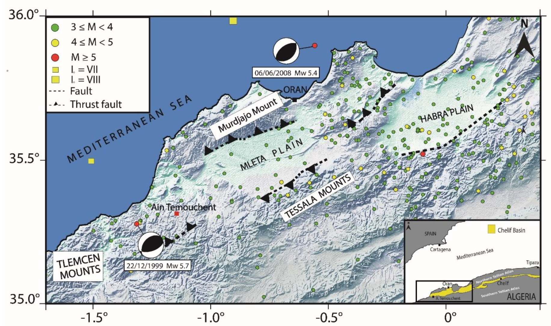
Figure 2.
The geological map of the Aïn Témouchent region, inspired from [9]. The blue circles indicate the single-station ambient noise measurement points, the green circles the array measurement points and the red circles the boreholes (as detailed in Table 1). The red numbered lines (1 to 6) correspond to cross-sections, and the black discontinuous line delineates the industrial zone. The bottom right panel illustrates the geometry used in the array measurements.
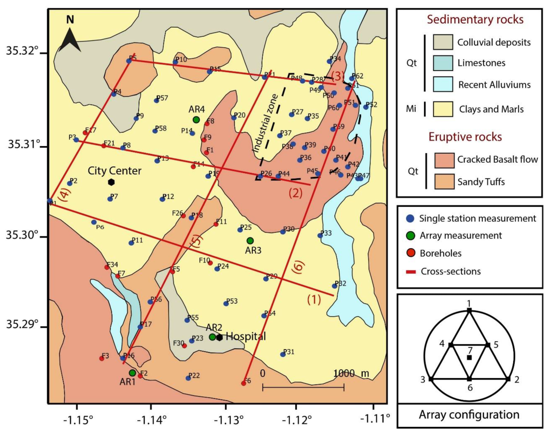
Figure 3.
Variation map of the fundamental frequency peaks () identified using the HVSR technique.
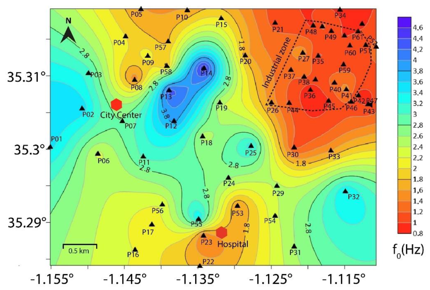
Figure 4.
The corresponding amplitude variation map () obtained by HVSR analysis.
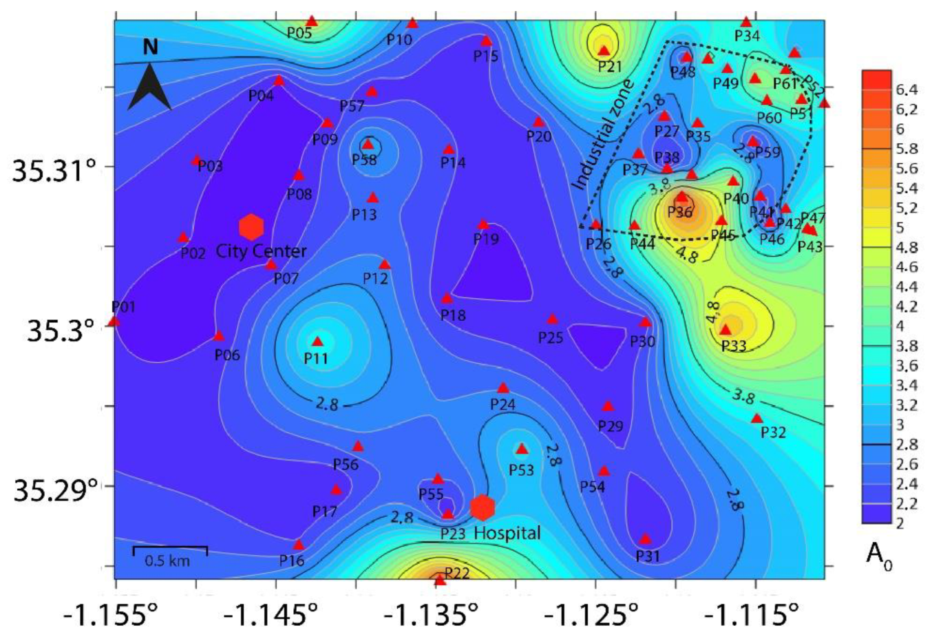
Figure 5.
Some examples of the experimental HVSR curves recorded at some selected sites in the studied region.
Figure 5.
Some examples of the experimental HVSR curves recorded at some selected sites in the studied region.
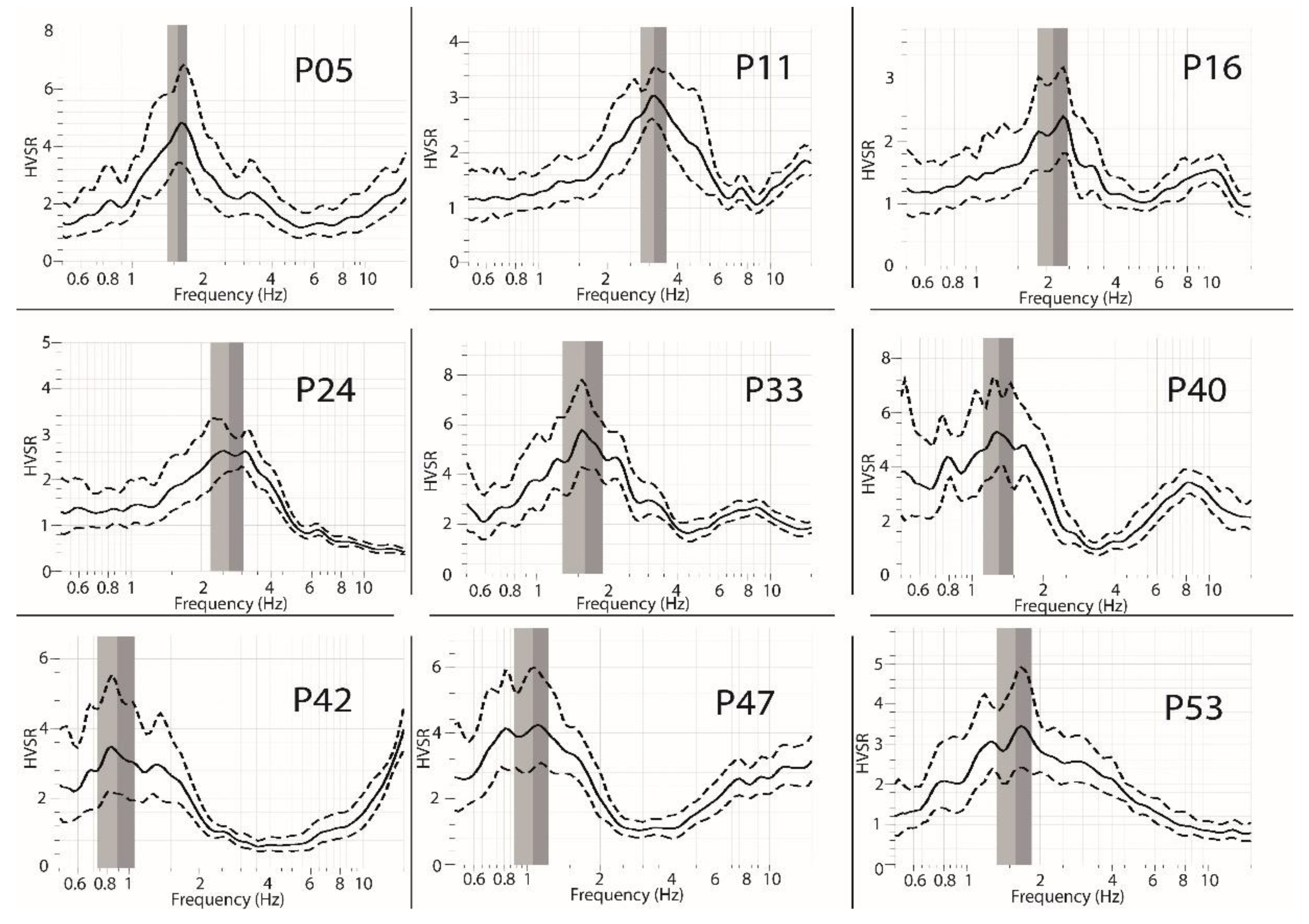
Figure 6.
Variation of the vulnerability index () for the city of Aïn Témouchent.
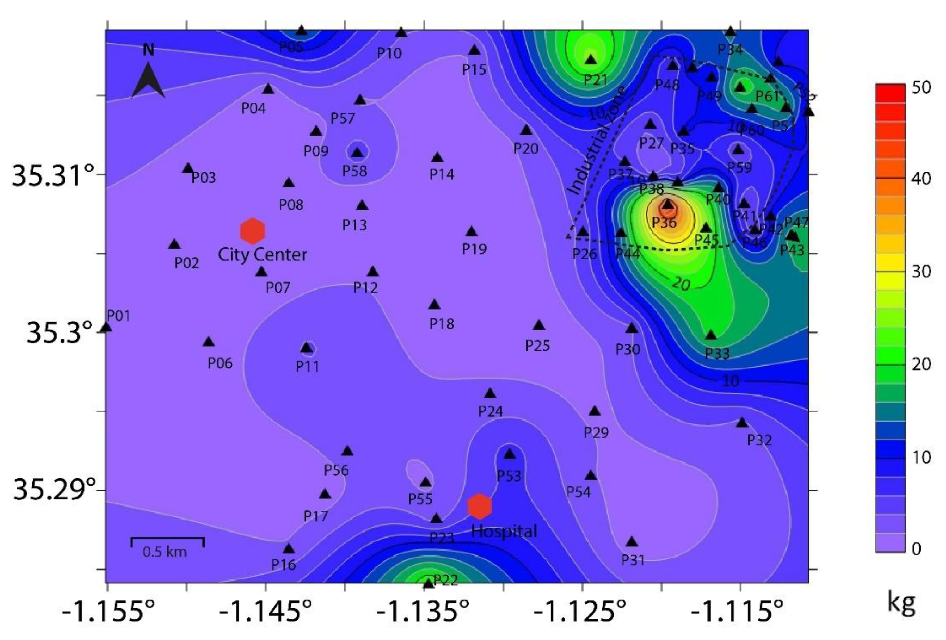
Figure 7.
(a) Obtained Rayleigh wave dispersion curves. Dark grey band represent dispersion curves solutions for minimum misfit +10 %. Light grey represent all the generated solutions. The two black lines represent the observed (black doted lines), and the calculated (with minimum misfit) dispersion curve, in black line. (b) The calculated Vs models (thick black line). Dark grey band represent Vs models with minimum misfit +10 %. Light grey represent all the generated models. The model with the minimum misfit is represented with a black line.
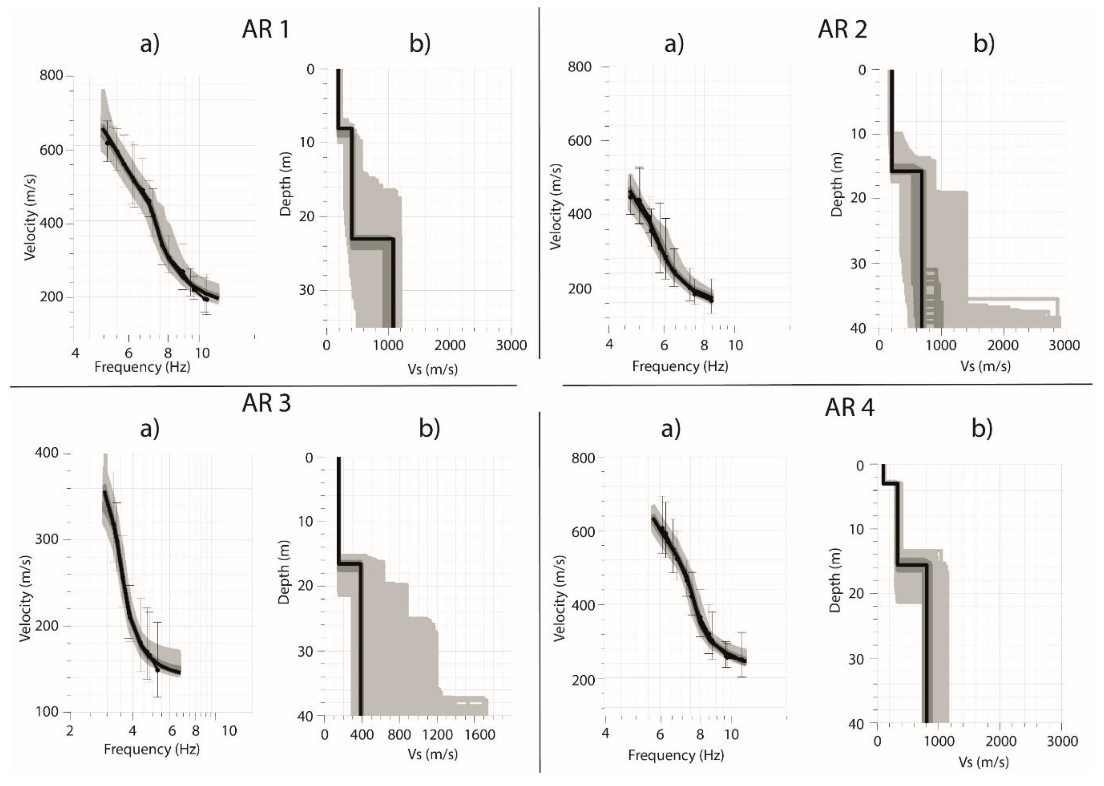
Figure 8.
Some results of the inversion of the HVSR curves. (Left) Experimental HVSR curve represented in black dotted line and fitted to the theoretical curve in red line. (Right) Estimated Vs models (black line). Dark grey band represent Vs models with minimum misfit +10 %. Light grey represent all the generated models. The model with the minimum misfit is represented with a black line in the right panels.

Figure 9.
2D cross-sections showing the lateral variation of different layers (a, c, e, g, i, k). The location and number of the profiles is presented in Figure 2 by red lines. Contour plot illustrating the correspondence between the fundamental frequency and the HVSR points, as a function of the corresponding amplitude (b, d, f, h, j, l).
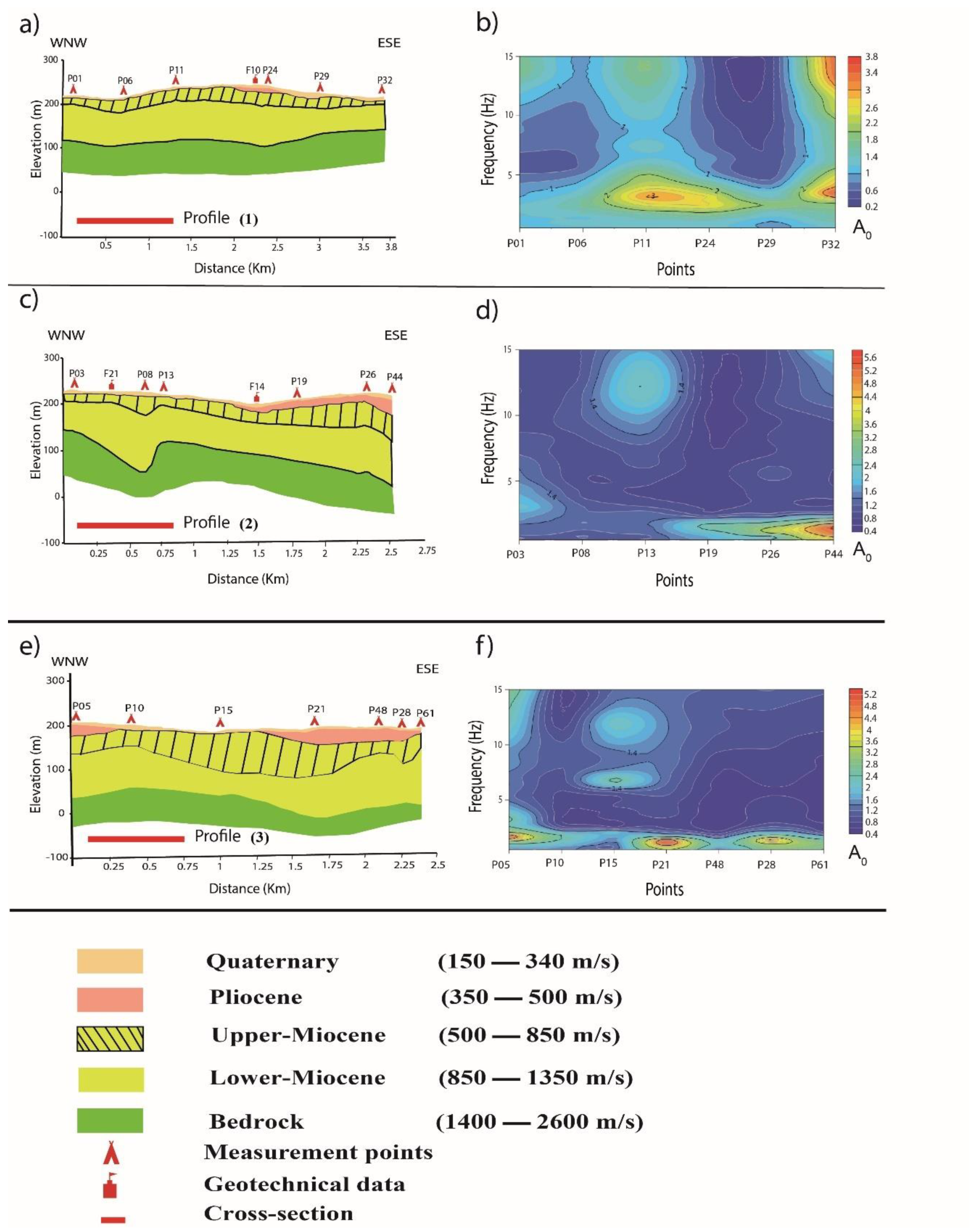
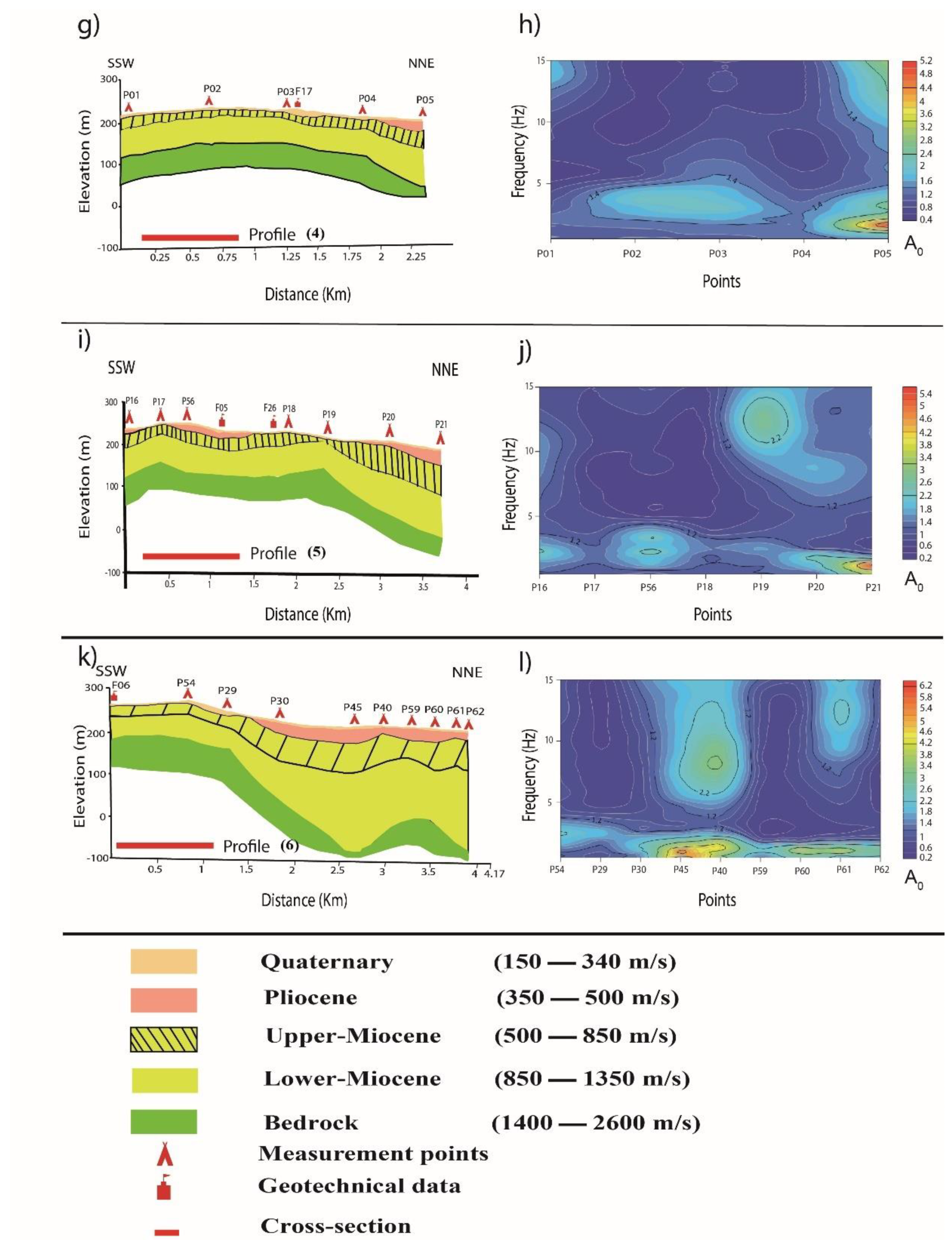
Figure 10.
Variation of the bedrock depth within the study area.
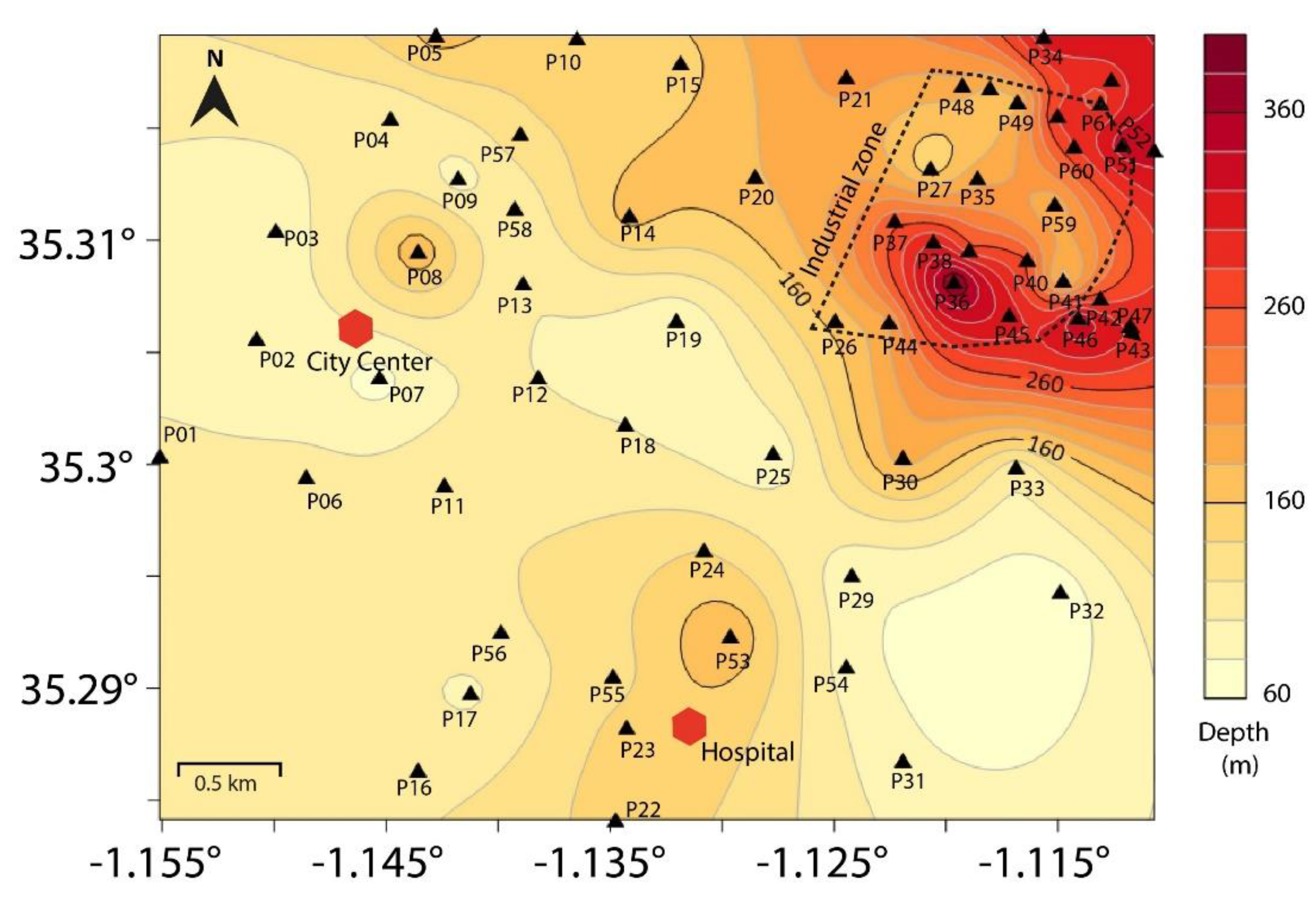
Figure 11.
Vs30 and soil classification in the city of Aïn Témouchent.
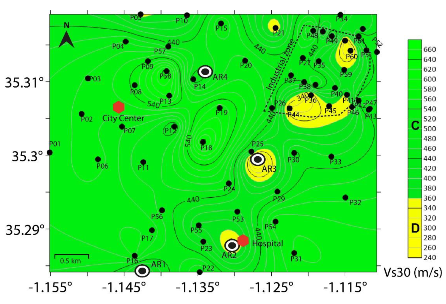
Figure 12.
The depth to bedrock is expressed as a function of the fundamental frequency, shown by the black line. In this relationship, and are the regression coefficients, is the fundamental frequency, is the depth to bedrock and R is the correlation coefficient.
Figure 12.
The depth to bedrock is expressed as a function of the fundamental frequency, shown by the black line. In this relationship, and are the regression coefficients, is the fundamental frequency, is the depth to bedrock and R is the correlation coefficient.
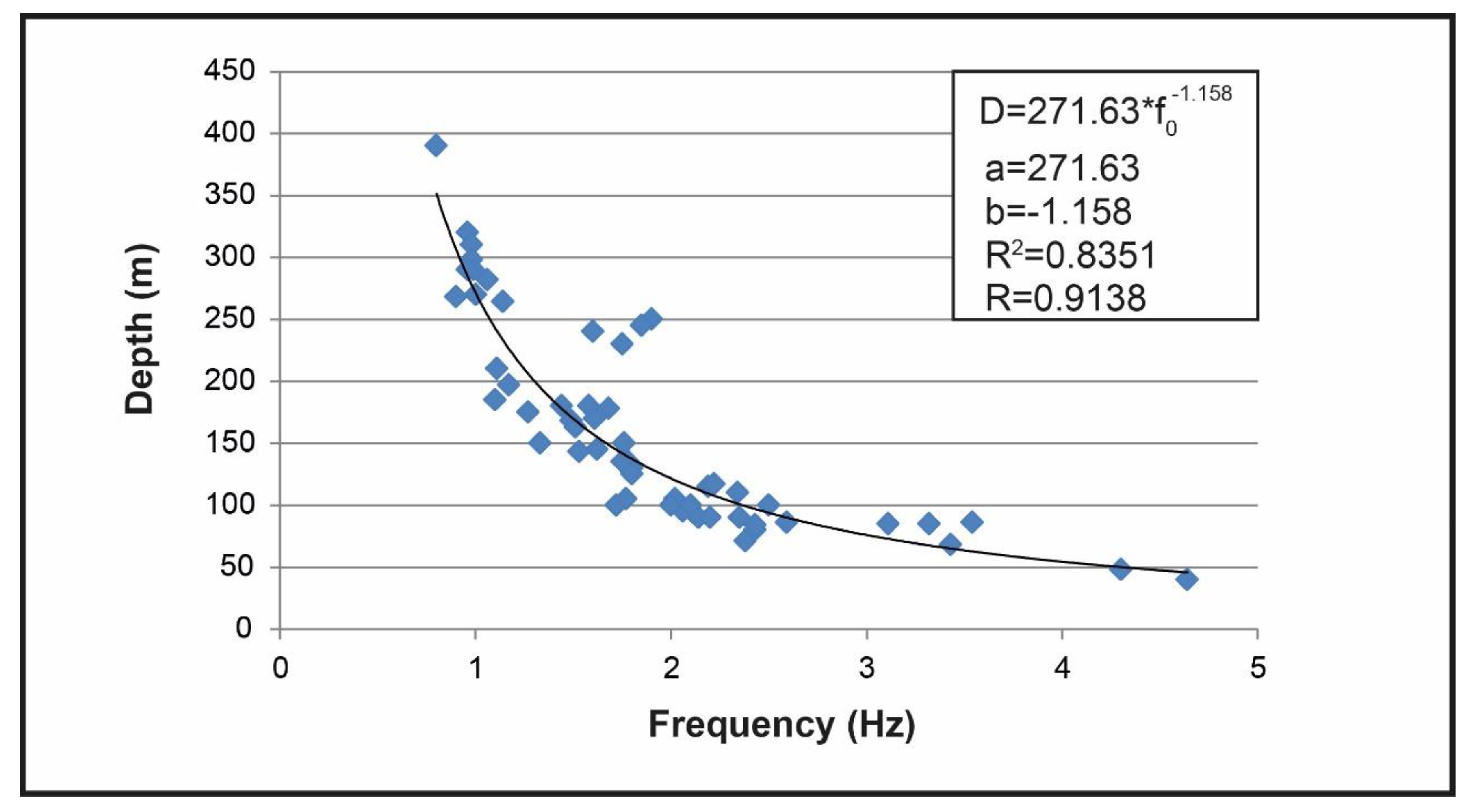

Table 1.
Layer structure from the available borehole information.
| Boreholes | Quaternary [m] | Pliocene [m] | Miocene [m] | |||
|---|---|---|---|---|---|---|
| F1 | 14 | .0 | > 13 | .0 | – | |
| F2 | 14 | .0 | 7 | .0 | 78 | .0 |
| F3 | 14 | .0 | 7 | .0 | 78 | .0 |
| F5 | 7 | .5 | > 10 | .0 | – | |
| F6 | 1 | .0 | – | > 35 | .0 | |
| F7 | 1 | .0 | – | > 19 | .0 | |
| F8 | 2 | .0 | > 9 | .5 | – | |
| F9 | 2 | .0 | 17 | .0 | > 2 | .0 |
| F10 | 4 | .0 | > 5 | .5 | – | |
| F11 | 4 | .0 | > 5 | .5 | – | |
| F14 | 1 | .0 | 4 | .0 | > 11.0 | |
| F17 | 8 | .0 | > 10 | .0 | – | |
| F21 | 2 | .0 | – | > 20 | .0 | |
| F26 | 1 | .0 | – | > 7 | .0 | |
| F30 | 7 | .5 | > 10 | .0 | – | |
| F34 | > 12 | .0 | – | – | ||
Table 2.
Input parameters for the inversion, including the number of layers and the ranges of Vp, Vs, and density.
Table 2.
Input parameters for the inversion, including the number of layers and the ranges of Vp, Vs, and density.
| Sedimentary Layers | Vp range [m/s] | Vs range [m/s] | Density range [kg/m3] |
|---|---|---|---|
| Quaternary | 150 — 1200 | 100 — 400 | 1600 — 2000 |
| Pliocene | 450 — 1650 | 300 — 550 | 1800 — 2100 |
| Upper-Miocene | 600 — 2700 | 400 — 900 | 1900 — 2200 |
| Lower-Miocene | 1200 — 4200 | 800 — 1400 | 2000—2400 |
| Bedrock | 2000 — 7000 | 1300 — 2750 | 2200 — 2800 |
Table 3.
NEHRP code for soil types and classification [31].
Table 3.
NEHRP code for soil types and classification [31].
| Vs (m/s) | Soil type | Classification of soil |
| Vs > 1500 | Hard rock | A |
| 760 < Vs ≤ 1500 | Rock | B |
| 360 < Vs ≤ 760 | Very dense soil and soft rock | C |
| 180 < Vs ≤ 360 | Stiff soil | D |
Disclaimer/Publisher’s Note: The statements, opinions and data contained in all publications are solely those of the individual author(s) and contributor(s) and not of MDPI and/or the editor(s). MDPI and/or the editor(s) disclaim responsibility for any injury to people or property resulting from any ideas, methods, instructions or products referred to in the content. |
© 2025 by the authors. Licensee MDPI, Basel, Switzerland. This article is an open access article distributed under the terms and conditions of the Creative Commons Attribution (CC BY) license (http://creativecommons.org/licenses/by/4.0/).
Copyright: This open access article is published under a Creative Commons CC BY 4.0 license, which permit the free download, distribution, and reuse, provided that the author and preprint are cited in any reuse.


