Submitted:
11 February 2025
Posted:
12 February 2025
You are already at the latest version
Abstract
Between 3 and 5 November 2019, mass movements occurred in Jericó, Antioquia, Colombia. Fortunately, no fatalities were reported during the events; however, five houses collapsed, two houses had damaged facade walls, and one power pole collapsed. Based on this, an analytical, probabilistic methodology is used to quantify the hazard intensity that occurred and affected the buildings. Initially, a technical description of the buildings and the damage caused is made. Three critical events are detected for hazard analysis, i.e. two related to landslides and one to debris flow. The hazard intensity is then quantified by determining the probabilistic parameters of velocity, dynamic thrust, momentum flux and overturning moment of the flow that caused damage to the different structures. These data are contrasted with the damage state thresholds for the overall behaviour of structures available in the literature. A structural fragility model in the out-of-plane direction in unreinforced masonry infill walls is used to obtain local complete damage thresholds. In addition, a complete damage threshold is calculated for the power pole. This study provides additional data that can strengthen knowledge related to the assessment of infrastructure risks associated with mass movements.
Keywords:
mass movements hazard intensity
; mass movements buildings' resistance
; mass movements vulnerability
; mass movements losses
; mass movements risk
; mass movements fragility curves
; damage thresholds
; unreinforced masonry
1. Introduction
Jericó is located to the southwest of the city of Medellín in the department of Antioquia, Colombia. There are reports compiled by the Colombian Geological Service where, since 1922, and on several occasions, events due to mass movements have been reported, repeatedly affecting the municipality's rural and urban areas [1,2,3,4]. From November 3 to 5, 2019, mass movements occurred, which caused significant damage to the population, private property and infrastructure [4]. Considering this event, an analytical and probabilistic methodology is used to quantify the mass movements' intensity and the affected buildings' physical vulnerability. There were two types of mass movements associated with the event: a debris flow from Las Nubes Hill, which was transported by the Valladares stream, saturated the sewage system and spread along Sixth Street to the municipal park, causing, among other damage, the collapse of a power pole. On Seventh and Ninth Streets, there were two landslides, which caused the collapse of five houses and damage to the facades of two others. The research considered the type of mass movements to calculate the velocity, dynamic thrust, momentum flux and overturning moment against the buildings. The Monte Carlo simulation technique was used to consider the uncertainty in the variables. The hazard intensity obtained was compared with the damage state thresholds for the overall behaviour of structures in the literature. For masonry walls subjected to out-of-plane loads and for a power pole, complete damage thresholds were obtained. These thresholds were compared with the hazard intensity to which they were subjected. Quantifying the intensity of mass movements related to the damage state of buildings is scarce and necessary information to obtain damage state thresholds and validate methodologies for calculating physical vulnerability and risk.
Figure 1.
(a) Risk area due to mass movements on the slope of Las Nubes Hill. Source: www.elmundo.com.co; (b) Mass movements November 3, 2019.
Figure 1.
(a) Risk area due to mass movements on the slope of Las Nubes Hill. Source: www.elmundo.com.co; (b) Mass movements November 3, 2019.
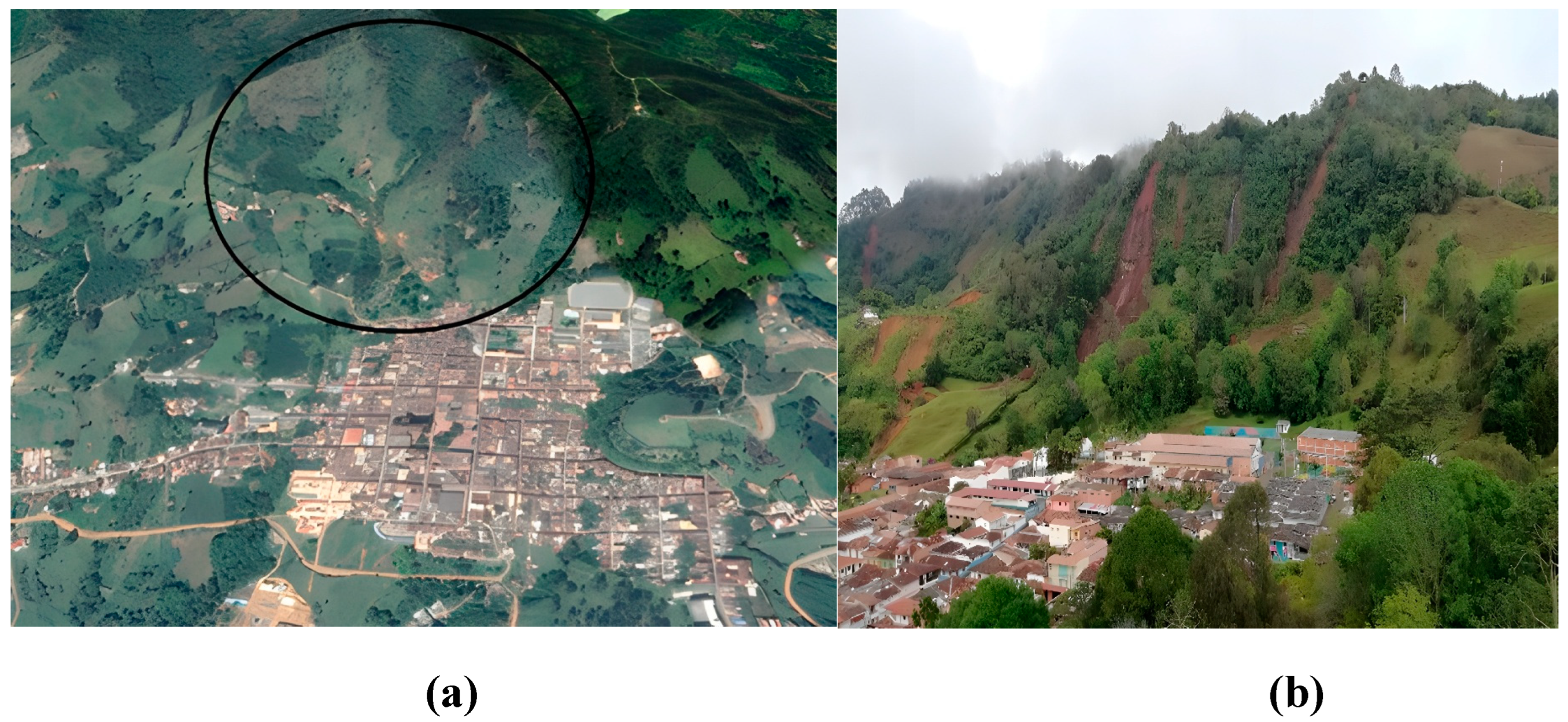
Figure 2.
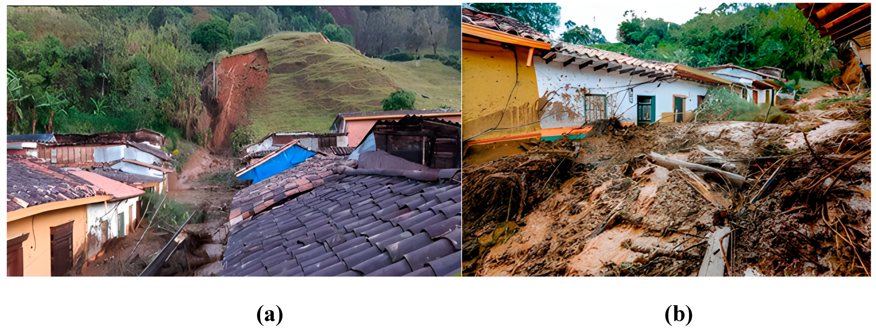
(a) Landslide. 1st Avenue - 6th – 7th Streets. www.eltiempo.com.co; (b) Landslide 1st avenue – 7th Street. Source: www.caracol.com.co.
Figure 2.
(a) Landslide. 1st Avenue - 6th – 7th Streets. www.eltiempo.com.co; (b) Landslide 1st avenue – 7th Street. Source: www.caracol.com.co.
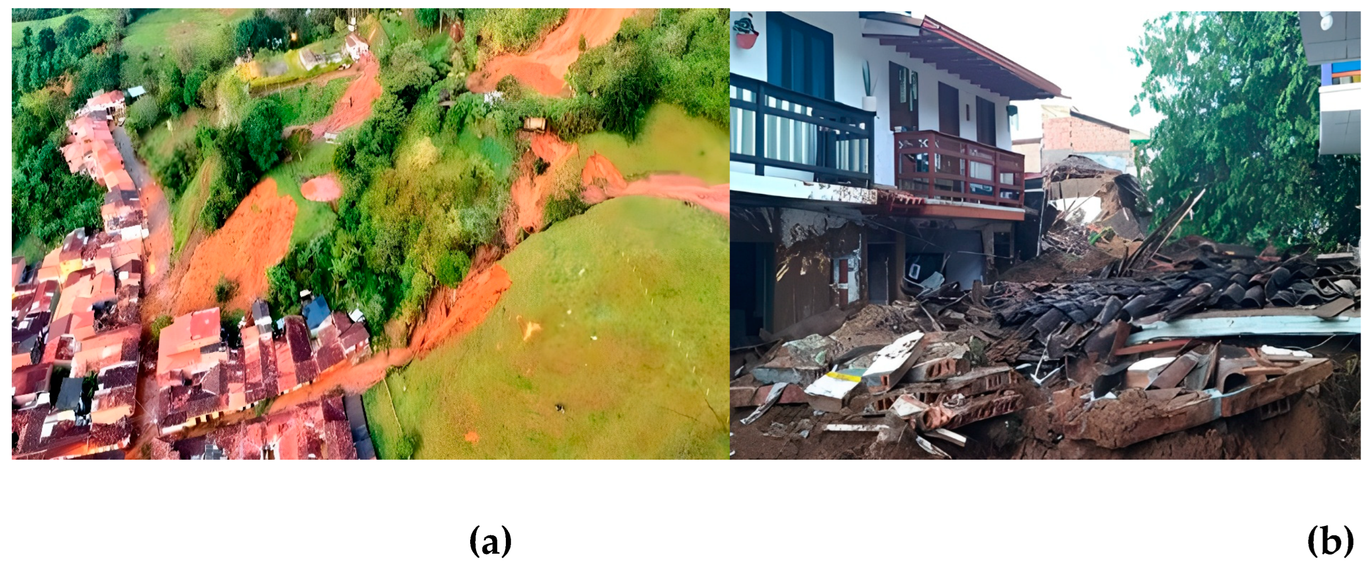
Figure 3.
(a) Debris flow. 1st Avenue – 6th Street. Source: twitter.com/Jericóantioq; (b) Debris flow 1st Avenue - 6th Street. www.eluniversal.com.co.
Figure 3.
(a) Debris flow. 1st Avenue – 6th Street. Source: twitter.com/Jericóantioq; (b) Debris flow 1st Avenue - 6th Street. www.eluniversal.com.co.
2. Damages Description to Affected Buildings
2.1. Demages Description House 1
House 1, shown in Figure 4, was directly impacted by the landslide to such an extent that the building collapsed, presenting a complete damage state considering references [5,6]. The single-storey dwelling was constructed of unreinforced clay brick masonry (URM) using horizontal perforated blocks of fired clay and a wooden roof with clay tiles. This building dissipated some of the energy that could reach House 2.
2.2. Damages Description House 2
A three-storey house (Figure 4) was built in an initial system of partially reinforced masonry. The walls comprise horizontal perforation blocks 10 cm wide, 20 cm high, 40 cm deep, 3.5 cm thick mortar, and a 1 cm one-sided plaster. At the time of impact, they were remodelling the first story of the building, for which they built a frame system with 25 x 25 cm columns and beams and a hollow clay block, reinforced concrete slab, as shown in Figure 4 and Figure 5. The building is in a light damage state based on [21,22]. The first-story infill walls were supported transversely on the new columns, and some walls collapsed due to their lack of flexural capacity when subjected to out-of-plane loads (Figure 5 and Figure 6). The span between columns is 2.9 m, and the height of the walls is 2.4 m. After the phenomenon, and probably as a solution to possible future stress due to mass movement, the construction of reinforced concrete walls on the first floor can be observed (Figure 5). These elements help in this type of event, but seismically, they are not necessarily favourable. It is interesting to note that the only infill wall that did not collapse, although cracked, of the four requested spans was the one that was transversely stiffened by the partitions that formed the kitchen of the neighbouring house (house 1) (Figure 6b).
2.3. Damages Description House 3
Figure 4 and Figure 7 show House 3. The house was built with horizontal perforation bricks; the structural system is partially reinforced with masonry. Due to the event, 50% of the building collapsed, including the kitchen and dining room areas. The dwelling damage is classified as extensive, considering references [21,22]. It can also be seen that the building was not hit head-on.
2.4. Damages Description House 4
Figure 8 shows the remains of the collapsed house. The single-storey building was structurally made of unreinforced clay brick masonry (URM). The bricks used were horizontal perforation blocks. The roof was made of wood and baked clay tiles. The building before the event is shown in Figure 9. This house was located at the intersection of 2nd Avenue and 9th Street. Based on [21,22], the present dwelling is classified as a complete damage state.
2.5. Damages Description House 5 to House 7
Figure 10 shows the only house that remained standing of the three houses across the street (left side) that were impacted head-on by the landslide. However, it is essential to recognise that the collision may have been mitigated, in part, by House 1, as shown in Figure 4. Plus, there is some degree of inclination, possibly favourable. This three-storey building, including the basement, whose predominant structural system is partially reinforced masonry, only damaged its main facade, Figure 10b. The facade consisted of wooden windows and masonry made of hollow horizontal cavity bricks without reinforcement. The collapsed wall had a span of 3.5 meters, as shown in Figure 10 and Figure 11. The damage in this dwelling, based on [5,6], is associated with a light damage state.
Figure 11a shows the rear of lot 6, the only uncollapsed portion of the building visible in Figure 11b. Eighty per cent of the building collapsed, and only vestiges of the roof are visible. About the part that remained standing, three floors of unreinforced masonry (URM) are observed. The walls are made of hollow clay bricks with the following measurements: 10 cm wide by 20 cm high and 40 cm deep, joined with mortar about 3.5 cm thick. Figure 12 shows in detail the remains of House 6. The two-storey collapsed section was supported by 20 cm x 20 cm concrete columns and an earth wall 50 cm thick (Figure 12 and Figure 13); on these elements rested a wooden mezzanine, which, being loose and subjected to the pressure of a landslide, contributed to the collapse of a large part of the building. In Figure 12b, some remains of the front part of the building can be seen along some wooden steps, a wooden wall, and an unreinforced masonry bathroom. Classifying the damage to the dwelling is associated with the complete damage state, according to [5,6]. House 7 (Figure 11b and Figure 12a) is associated with the complete damage state, taking into account [5,6]. This two-storey building was structurally supported by unconfined masonry (URM).
2.6. Damage Description to Houses Located on Sixth Street and the Lower Part of the Slope of Cerro las Nubes
Since a large part of the debris flow coming from Las Nubes hill was channelled through the Valladales stream, entering from the front on Sixth Street, the road served as a channel dissipating a large amount of energy along the street until almost reaching the principal Park (Figure 3, and 15). A large amount of mud penetrated the first houses through doors and windows, which the community extracted. Nevertheless, although there are economic losses at the finishes and additional works level, there is no evidence of structural damage in the dwellings (Figure 15b and Figure 16). A power pole collapsed due to the impact of the debris flow, Figure 14. The damage classification of the houses located on Sixth Street and the lower part of the slope of Las Nubes Hill, based on [5,6], is associated with the light damage state.
3. Theoretical Framework for the Mass Movements Velocity Calculation
For decades, several professionals, due to the socio-environmental and economic problems caused by mass movements, have been concerned with understanding and reducing the phenomenon, so researchers such as [7,8,9,10,11,12] have published several empirical formulations correlated with different mass movement phenomena in specific places. In these researches, the study of parameters such as the potential volume of debris, mean flow velocity, maximum discharges, and the distance or path of the flow gained significant interest. Mass movements can carry different materials; therefore, determining the appropriate roughness coefficients is difficult. It is essential to understand that the friction between the materials that make up the mass movements and the supporting surface causes the energy to dissipate faster than water flow circulation [13].
Deducing the mass movement velocity at the instant of collision is essential for calculating the stresses acting on any surface. Taking into account the type of flow and its dynamic behaviour along the path, applicable experimental deductions have been made in analytical and numerical methodologies [9,11,13,14,15], Error! Reference source not found. and Eq. (13).

Table 1.
Equations to estimate mass movements velocity.
| Reference | Equation | |
| Newtonian laminar flow | (1) | |
| Hungr’s equation [7,16] | (2) | |
| Manning – Strickler equation | (3) | |
| Yang’s equation [11,17] | (4) | |
| Du’s equation [13] | (5) | |
| Chézy equation [8] | (6) | |
| Empirical equation [8] | (7) | |
| Lo’equation [16,18] | (8) | |
| Prochaska’s equation [19] | (9) | |
| Hu’s equation [10] | (10) | |
| Yang’s equation [11] | (11) | |
| Wang’s equation [12] | (12) |
Note: The abbreviation and symbol used in Table 1 have been described at the manuscript's end.
Table 2.
Relationship between the coefficient k1 and the depth of the debris flow.
| H (m) | <2.5 | 2.75 | 3 | 3.5 | 4 | 4.5 | 5 | >5.5 |
| K1 | 10 | 9.5 | 9 | 8 | 7 | 6 | 5 | 4 |
Table 3.
Chézy coefficient, for Newtonian or near Newtonian flows.
| Type | C | |
| Water, smooth channel | 0.0025 | |
| Mudflow | 0.002 | |
| Pinatubo - mudflow | 0.0024 | |
| Sediment laden flow | 0.005 | |
| Pinatubo - hyper-concentrated flow | 0.009-0.014 | |
| Mangatoetoenui - lahar | 0.02 - 0.1 | |
| Pinatubo - lahar | 0.01 - 0.3 | |
| Lahars | 0.01 - 1 | |
| Debris flow | 0.06 - 0.577 | |
| Wet landslide | 0.184 |
4. Theoretical Framework for the Calculation of Mass Movements Dynamic Thrust against Buildings
Hungr et al. (1984) [7] present perhaps the most famous hydrodynamic formulation to quantify mass movement hitting against a vertical barrier [23]. The authors determine that the mass movements dynamic thrust can be calculated with Eq. Error! Reference source not found. for barriers almost perpendicular to the flow direction. The hydrodynamic model's dimensionless impact coefficient (k) is 1.50. This value depends on the grain size distribution of the flow [24,25].
Below are some experimentally developed hydrostatic and hydrodynamic models for calculating the pressure from mass movements against vertical barriers.
Table 4.
Hydrodynamic and hydrostatic hydraulic models.
| Reference | Equation | |
| Zhang (1993) | (25) | |
| Armani (1997) | (16) | |
| Scotton and Deganutti (1997) | (17) |
A dynamic pressure coefficient (k) equal to 2.5 is adjusted to the mean impact pressure due to mass movement, considering boulders with diameters up to 0.5 meters [18,27]. If larger diameters are present, the effect of the dynamic impact of mass movement and boulders should be calculated separately.
Table 5 shows experimentally developed mixed models for calculating mass movement pressure in vertical barriers. After identifying the strengths and weaknesses of hydrostatic and hydrodynamic models, researchers conclude that mixed models seem to be the best method to predict the pressure exerted by mass movements on a barrier [14]; they establish that the impact pressure can be calculated using Eq. Error! Reference source not found..
5. Theoretical Framework for Structural fragility curves
Fragility curves represent the probability of reaching or exceeding a specified limit damage state when a structure is subjected to a given hazard intensity. In the following definition, momentum flux was used as the intensity parameter (Eq, (23)). Nevertheless, other variables, such as height (h) or overturning moment (h2v2), can also be used. Log-normal functions are proposed as mass movement fragility curves using the momentum flux, hv2 (where h and v are the height and velocity of mass movement at a given site, respectively) as the hazard intensity parameter [30]. Each curve is characterised by a median value and its log-normal standard deviation (β). Therefore, the probability of reaching or exceeding a specific damage state, given a structural response due to a defined hazard (mass movements), can be calculated as follows:
Which denotes a cumulative logarithmic normal distribution, where:
: the mass movement impact index represents the intensity of the hazard.
: it is the median value of the impact index at which the building reaches the Damage State (DS).
: it is the standard deviation of the natural logarithm of the impact index associated with a Damage State (DS).
Φ: it is the standard normal cumulative distribution function.
These curves are defined by two parameters: the median value and the standard deviation . The median value defines the point at which the probability of equaling or exceeding the damage state equals 50%, and the standard deviation gives an idea of the scatter.
6. Calculations and Results Analysis
This item aims to find measures of velocity, dynamic thrust, momentum flux, overturning moment, and structural fragility parameters. The research refers to three events. The one on First Avenue with Seventh Street related to the landslide of a slope collapsing houses 1, 6, and 7 referenced in item 2 (Figure 4 and Figure 11). The one that occurred at the junction of Second Avenue with Ninth Street due to the landslide of a slope collapsing a house (Figure 8 and Figure 9), and what happened at the intersection of Sixth Street with Las Nubes hill regarding debris flows channelled over the Valladales stream, reaching Sixth Street, and travelling to the vicinity of the central municipal park (Figure 3).
6.1. Calculation of Flow Velocity in Collapsed Houses
The events that occurred at First Avenue and Seventh Street and the one at the intersection of Second Avenue and Ninth Street are related to the landslide of a block of soil adjacent to the houses (Figure 4 and Figure 13), triggered, among other reasons, by the high rainfall in the area. For this reason, Eq. (13) consistently calculates the velocity. Due to the uncertainty of the phenomenon, a probabilistic analysis using Monte Carlo simulation is required. According to the different variables visible in Eq. (13), this research chooses to use the continuous uniform probability distribution function since, among other functions, it provides maximum entropy when only extreme data are available. Table 6 shows the variables referred to. For the dynamic soil friction coefficient (φ), this research uses values referenced in RM Iverson, 1997 [31].
6.2. Calculation of Thrust and Acting Momentum Flux Collapsed Houses
Following recommendations of FEMA, 2017 [6], using Eq. (22), the variables with their respective setting functions are recognised in Table 9. The variables and their uncertainties referring to the mass movements, such as density (ρ), drag coefficient (Cd), and impact coefficient due to debris size (kd), are obtained according to [6,30]. The flow height during impact (h) is a time-varying measure. The research uses a continuous uniform fit function for its representation, which expresses the maximum entropy.
6.3. Collapsed Infill Walls First Floor, House 2
House 2 had no significant structural overall damage; however, some facade lateral walls collapsed in the first story, Figure 4. Unreinforced masonry infill walls (Figure 6) were forced by the landslide to an out-of-plane stress phenomenon, as shown in Figure 18. Although unconfined and unreinforced masonry offers little resistance to this event, damage thresholds will be calculated below. The first-story partition walls in house 2 collapsed a few meters away from houses 1, 6, and 7, analysed previously. Therefore, the magnitudes and other probabilistic data will be helpful.
6.3.1. Calculation of Acting Momentum Flux in Collapsed Infill Walls, House 2
6.3.2. Infill walls fragility curve due to out-of-plane loads by the landslide
Since the 50s, different analytical, numerical, and experimental studies have been carried out regarding the out-of-plane direction strength of the unreinforced masonry walls [32,33,34,35,36,37,38,39,40,41,42,43,44,45,46,47,48]. Consistent with [49] y [37], the damage thresholds in walls subjected to out-of-plane loads in the present research are calculated considering the study carried out by [41]. Abrams et al., 1996 [41] assumed the wall resists a uniform lateral load through a one-way arch mechanism. Therefore, researchers determine the ultimate strength of the out-of-plane walls, as seen in Eq. (24). Asteris et al., 2017 [50] present a best-fitting equation for calculating the coefficients for fixed H/t ratios; see Eq. (25).
The ultimate capacity of the wall is equated; see Eq. (24), with the request due to the landslide visible in Eq. (22). If all field parameters are known, see Table 12 and Table 14. Through techniques such as Monte Carlo, a function log-normal analytical is obtained regarding momentum flux (hv2), determining complete damage thresholds in walls subjected to out-of-plane loads (Table 13 and Table 15).
The median value capacity in terms of momentum flux for a complete damage state in infill walls house 2 is approximately 0.46 m3/s2 (Table 15), which is essential to explain the collapse of these structures when compared to the median value of momentum flux acting on the infill walls of 40.63 m3/s2, as referred in item 6.3.1.
6.4. Collapsed Power Pole Analysis
The only structure that collapsed at the intersection of Sixth Street and Las Nubes Hill was a power pole. This element is used as a calibration to obtain parameters of velocity, dynamic thrust, momentum flux, and overturning moment (Figure 14) to generate knowledge that helps objectively interpret this kind of event.
The power pole was 8 m high and had a reinforced concrete cross-section, as shown in Figure 21; the reinforcement consisted of 8 longitudinal bars ½ in each and 4 mm diameter stirrups (wire) located every 11 cm.
6.4.1. Calculation of Flow Velocity, Collapsed Power Pole
A probabilistic analysis using Monte Carlo simulation was performed to calculate the debris flow velocity at 40 meters from Sixth Street's intersection and Cerro Las Nubes's slope. The formulations shown in Table 1 are used for channelised debris flows such as the one that occurred on Sixth Street (see Figure 3), considering equal probabilistic weight for each equation. Table 16 shows the variables used in the velocity calculation, their randomness, and the respective setting functions.
The contact width of the debris flow over pole (B) equals 0.38 m, deduced as half perimeter, and the slope of Sixth Street (S) equals 0.054. The above are known parameters. According to the Kolmogorov-Smirnov statistical criterion (K-S test), the General Beta function is the one that best fits the actual data for the calculation of the velocity, obtaining the statistics shown in Table 16. This information is relevant to continue the probabilistic analysis of the thrust acting on the collapsed power pole (Table 17).
6.4.2. Calculation of the Debris Flow Dynamic Thrust on the Collapsed Power Pole
Following the recommendations of FEMA, 2017 [6], and using Eq. (22), Table 18 shows the variables used with their respective setting functions..
The variables in Table 18 referring to density (ρ), drag coefficient (Cd), and impact coefficient due to debris size (kd) are obtained according to [6,30]. The debris flow height at the moment of impact (h) is a time-varying measure; in the present research, a continuous uniform fit function is used to represent maximum entropy. Under the Kolmogorov-Smirnov statistical criterion (K-S test), the Lognormal and Pert functions efficiently fit the actual data for the calculation of thrust, momentum flux, and overturning moment, respectively, obtaining the statistical data shown in Table 19, Table 20 and Table 21.
6.4.3. Development of the Power Pole Complete Damage Threshold due to Debris Flow
The power pole is impacted at the base by the debris flow and response in terms of shear strength, according to Eq. (26). This expression is used following recommendations of ACI 318 2014 for circular sections in reinforced concrete [51]. Where b is equal to the diameter of the cross-section and d corresponds to 0.8b. Since the transverse reinforcement found was insignificant, its contribution to shear strength is not considered. Continuing a probabilistic analysis, Table 22 shows the variables used, knowing that the cross-section of these power poles is hollow. Using the Monte Carlo technique, a cumulative log-normal function representative of the shear capacity is obtained, see Table 23, transcendental information to match with hazard and find a cumulative log-normal function in terms of momentum flux (hv2). Look at Table 24 and Table 25.
To check the bending capacity of the power pole according to [51] Eq. (27) is used, considering that the gravitational axial load applied to the power pole is less than 10% of Agf'c.
Where represents the nominal bending strength in the section. it represents the area of the longitudinal reinforcement. is the specified yield strength of the reinforcement. Z, equal to 0.7b, is the distance between the points of application of the resulting forces tensile and compression.
Equating capacity with demand makes it possible to obtain an analytical expression regarding overturning moment (h2v2). Table 26 shows the variables used. Through Monte Carlo simulation, a log-normal cumulative function is obtained that represents a complete damage threshold for power poles such as the one found in Jericó, having as intensity the overturning moment due to debris flows (see Table 27).
7. Discussion
This research provides information on flow intensity parameters, including velocity, dynamic thrust, momentum flow and overturning moment, between 3 and 5 November 2019 in Jericó, Antioquia, Colombia. It also provides a technical description of the structural damage to the impacted buildings. In addition, it includes information on the structural fragility of unreinforced masonry buildings in the municipality due to mass movements.
The median thrust for houses 1, 6, and 7 is 841.8 kN, and for house 4, it is 556.64 kN (Table 10). The median momentum flux for houses 1, 6, and 7 is 81.26 m3/s2, and for house 4, it is 50.89 m3/s2 (Table 11). This is contrasted with the median momentum flux threshold of 23.30 m3/s2 for a complete damage state in URM Colombian structures [30], which supports the collapse of the unreinforced masonry houses studied.
Although the damage to house number two was slight, some facade walls collapsed because they were forced to flex out-of-plane due to the landslide. The median momentum flux that caused the walls to collapse was 40.63 m3/s2, contrasted with a complete damage threshold equal to 0.46 m3/s2. This analysis reiterates the inability of unreinforced masonry to assume flexion out-of-plane. Although these types of local failures in a building must be analysed, it is essential to appreciate that the partially confined masonry building's overall stability was maintained. The three-story building also has a reinforced concrete frame system at the first-story level, giving it additional strength. It must be recognised that part of the lateral load with which this building was analysed (house 2) was dissipated by the collapsed house, number 1.
Electricity, among other services, is vital even in atypical situations such as those generated by debris flows. However, for the event that occurred in Jericó, the collapse of a power pole was observed under a medium thrust of 21.01 kN, a median momentum flux of 33.98 m3/s2, and a median overturning moment of 51.09 m4/s2. Contrasting complete damage thresholds with a shear median capacity of 18.13 kN, a median momentum flux of 28.87 m3/s2, and a median overturning moment of 56.46 m4/s2. According to what was observed on the ground, the hydraulic concrete of the power pole failed at the base when the shear force of the debris flow impacted it.
Considering the different variables and the uncertainty in calculating intensity and structural fragility, it was decided to do a probabilistic analysis using Monte Carlo simulation. It is necessary to know the different variables to reduce uncertainty by taking advantage of prior knowledge and field data. The technique illustrated in this work allows the probability calculation of hazard intensity, structural fragility, and risk against mass movements.
8. Conclusions
The research offers field data, hazard intensity measurement, damage auscultation, and thresholds of structural damage due to mass movements, according to what happened in Jericó, Antioquia, Colombia. This information is expected to help advance the probabilistic quantification of the hazard intensity, vulnerability, and risk due to mass movements, contributing to risk reduction through knowledge ownership.
Author Contributions
conceptualization, A.L.S-C., J.A.P., J.W.B; methodology, A.L.S-C., J.A.P., J.W.B; software, A.L.S-C., J.A.P., J.W.B; validation, A.L.S-C., J.A.P., J.W.B; formal analysis, A.L.S-C., J.A.P., J.W.B; investigation, A.L.S-C., J.A.P., J.W.B; resources, A.L.S-C., J.A.P., J.W.B; writing—original draft preparation, A.L.S-C., J.A.P., J.W.B; writing—review and editing, A.L.S-C., J.A.P., J.W.B; visualisation, A.L.S-C., J.A.P., J.W.B; supervision, A.L.S-C., J.A.P., J.W.B. All authors have read and agreed to the published version of the manuscript.
Funding
this research received external funding from the Ministry of Science, Technology, and Innovation (COLCIENCIAS) as part of the Bicentennial Scholarship Program.
Institutional Review Board Statement
not applicable.
Informed Consent Statement
not applicable.
Data Availability Statement
data is available on reasonable request to the corresponding author.
Acknowledgments
the authors gratefully acknowledge the support provided by Dr Carlos Estuardo Ventura (Professor of Civil Engineering and Director of EERF The University of British Columbia), Dr Juan Diego Jaramillo Fernández (Retired Emeritus Professor School of Applied Sciences and Engineering EAFIT University, Colombia).
Conflicts of Interest
the authors declare no conflict of interest.
Symbols
| As | Area of longitudinal tensile reinforcement |
| : | The median value of the impact index at which the building reaches the threshold of a damage state |
| b | The diameter of the cross-section |
| B | Barrier element width. The mass movement direction is perpendicular to this dimension |
| C | Chezy coefficient |
| cd | Drag coefficient |
| Cv | Sediment volumetric concentration |
| d | Corresponds to 0.8b |
| db | The diameter of the longitudinal reinforcement |
| De | Cross external diameter |
| Di | Cross internal diameter |
| f'c | Specified compressive strength of the concrete |
| f'm | Specified compressive strength of the masonry |
| Fu | The ultimate strength |
| fy | Yield strength of the longitudinal reinforcement |
| h | Mass movement depth |
| H | Wall effective height |
| h’ | Vertical measurement of the landslide |
| hv2 | Momentum flux or impact index |
| h2v2 | Overturning moment |
| Kd | Impact coefficient |
| L | Wall length |
| Mn | The nominal bending strength in the section |
| p(%) | The clay content of sedimentary material |
| qult | The ultimate strength of the out-of-plane walls |
| S | The bed slope where the stream flows |
| t | The effective thickness of the wall |
| v | Mass movement frontal velocity |
| V | Concrete shear strength |
| Z | Distance between the points of application of the resulting forces tensile and compression |
| β | The standard deviation of the natural logarithm of a variable |
| βDS | Standard deviation of the natural logarithm of the impact index associated with a damage state |
| ρ | Mass movement density |
| Φ | The standard normal cumulative distribution function |
| Abbreviations | |
| URM | Unconfined, unreinforced clay brick masonry |
| sd | The standard deviation of a variable |
| Probability of reaching or exceeding a specific damage state, given a structural response due to a defined hazard (mass movements) | |
References
- S. de planeación y desarrollo Municipio de Jericó, “Formulación del Esquema de Ordenamiento Territorial,” vol. 011, no. 072. p. 145, 2010. [Online]. Available: chrome-extension://efaidnbmnnnibpcajpcglclefindmkaj/https://staticprd.minuto30.com/wp-content/uploads/2020/03/E.O.T.-JERICO.pdf.
- H. Barrientos Velasquez and M. T. Vasquez Restrepo, “Zonas de amenaza en la jurisdicción de la corporación autónoma regional del centro de Antioquia.” p. 105,106, 1996. [Online]. Available: chrome-extension://efaidnbmnnnibpcajpcglclefindmkaj/https://cia.corantioquia.gov.co/ciadoc/GESTION_DEL_RIESGO/GA_GESTIONAMBIENTAL_244REG_1996.pdf.
- Alcaldía de Jericó, Documento Formulación Esquema de Ordenamiento Territorial (EOT) Municipio de Jericó. 2019. [Online]. Available: https://jericoantioquia.micolombiadigital.gov.co/sites/jericoantioquia/content/files/000123/6105_formulacion_jerico_2019-mod-mpio.pdf.
- D. M. Á. Michael Steve Rangel Florez, Jesús García Núñez, Report of the emergency visit to the municipality of Jericó - Antioquia., no. November 2019. 2019, p. 49. [Online]. Available: https://www.researchgate.net/publication/378489786_INFORME_DE_VISITA_DE_EMERGENCIA_EN_EL_MUNICIPIO_DE_JERICO-ANTIOQUIA.
- Federal Emergency Management Agency (FEMA), HAZUS-MH MR4 Technical Manual. 2003.
- F. E. M. A. FEMA, Hazus Tsunami model technical guidance, no. November. 2017, p. 171. [Online]. Available: https://www.fema.gov/sites/default/files/2020-09/fema_hazus_tsunami_technical-manual_4.0.pdf.
- O. Hungr, G. C. Morgan, and R. Kellerhals, “Quantitative analysis of debris torrent hazards for design of remedial measures.,” Can. Geotech. J., 1984, doi: 10.1139/t84-073.
- D. Rickenmann, “Empirical relationships for debris flows,” Nat. Hazards, 1999, doi: 10.1023/A:1008064220727.
- A.B. Prochaska, P. M. Santi, J. D. Higgins, A. B. Prochaska, P. M. Santi, and J. D. H. Gins, “Relationships between size and velocity for particles within debris flows,” Can. Geotech. J., 2008, doi: 10.1139/T08-088.
- K. Hu, M. Tian, and Y. Li, “Influence of Flow Width on Mean Velocity of Debris Flows in Wide Open Channel,” J. Hydraul. Eng., vol. 139, no. 1, pp. 65–69, 2013, doi: 10.1061/(asce)hy.1943-7900.0000648.
- H. Yang, F. Wei, and K. Hu, “Mean velocity estimation of viscous debris flows,” J. Earth Sci., 2014, doi: 10.1007/s12583-014-0465-z.
- T. Wang, J. Chen, X. Chen, Y. You, and N. Cheng, “Application of incomplete similarity theory to the estimation of the mean velocity of debris flows,” Landslides, 2018, doi: 10.1007/s10346-018-1045-6.
- J. Suárez, Control de erosión en zonas tropicales. 2001. [Online]. Available: https://www.erosion.com.co/control-de-erosion-en-zonas-tropicales/.
- X.-L. Gong et al., “Characteristics of a Debris Flow Disaster,” Water, vol. 12, no. 1256, pp. 1–25, 2020, doi: 10.3390/w12051256.
- A.M. Ramos Cañón et al., Methodological Guide for Torrential Flood Hazard Zoning. Bogotá D. C., Colombia, 2021. [Online]. Available: https://www.researchgate.net/publication/362001780_Guia_metodologica_para_evaluacion_de_amenaza_por_avenidas_torrenciales.
- D. O. . Lo, “Review of natural terrain landslide debris-resisting barrier design,” 2000. [Online]. Available: https://www.cedd.gov.hk/eng/publications/geo/geo-reports/geo_rpt104/index.html.
- P. Cui, G. G. D. Zhou, X. H. Zhu, and J. Q. Zhang, “Scale amplification of natural debris flows caused by cascading landslide dam failures,” Geomorphology, vol. 182, no. October 2017, pp. 173–189, 2013, doi: 10.1016/j.geomorph.2012.11.009.
- J. Peng et al., “Heavy rainfall triggered loess-mudstone landslide and subsequent debris flow in Tianshui, China,” Eng. Geol., vol. 186, pp. 79–90, 2015, doi: 10.1016/j.enggeo.2014.08.015.
- A.B. Prochaska, P. M. Santi, J. D. Higgins, and S. H. Cannon, “A study of methods to estimate debris flow velocity,” Landslides, 2008, doi: 10.1007/s10346-008-0137-0.
- M. H. Bulmer, O. S. Barnouin-Jha, M. N. Peitersen, and M. Bourke, “An empirical approach to studying debris flows: Implications for planetary modeling studies,” J. Geophys. Res. E Planets, vol. 107, no. 5, 2002, doi: 10.1029/2001je001531.
- Q. Zhong and Q. Yue, Dynamics of Large and Rapid Landslides with Long Travel Distances Under Dense Gas Expanding Power, vol. 3. 2014. doi: 10.1007/978-3-319-04996-0_17.
- G. Ávila et al., Methodological guide for studies of hazard, vulnerability, and risk due to mass movements. 2016. doi: 10.32685/9789589952856.
- P. Cui, C. Zeng, and Y. Lei, “Experimental analysis on the impact force of viscous debris flow,” Earth Surf. Process. Landforms, vol. 40, no. 12, pp. 1644–1655, 2015, doi: 10.1002/esp.3744.
- F. Vagnon and A. Segalini, “Debris flow impact estimation on a rigid barrier,” Nat. Hazards Earth Syst. Sci., vol. 16, no. 7, pp. 1691–1697, 2016, doi: 10.5194/nhess-16-1691-2016.
- S. Poudyal et al., “Review of the mechanisms of debris-flow impact against barriers To cite this version : HAL Id : hal-02923131 Review of the mechanisms of debris-flow impact against barriers,” 2020, [Online]. Available: chrome-extension://efaidnbmnnnibpcajpcglclefindmkaj/https://hal.science/hal-02923131/document.
- K. Hu, F. Wei, and Y. Li, “Real-time measurement and preliminary analysis of debris-flow impact force at Jiangjia Ravine, China,” Earth Surf. Process. Landforms, vol. 36, no. 9, pp. 1268–1278, 2011, doi: 10.1002/esp.2155.
- R. Koo, “A Review on the Design of Rigid Debris-resisting Barriers,” no. January, 2018, [Online]. Available: https://www.cedd.gov.hk/eng/publications/geo/geo-reports/geo_rpt339/index.html.
- J. A. Prieto, M. Journeay, A. B. Acevedo, J. D. Arbelaez, and M. Ulmi, “Development of structural debris flow fragility curves (debris flow buildings resistance) using momentum flux rate as a hazard parameter,” Eng. Geol., 2018, doi: 10.1016/j.enggeo.2018.03.014.
- J. W. Kean et al., “Inundation, flow dynamics, and damage in the 9 January 2018 Montecito debris-flow event, California, USA: Opportunities and challenges for post-wildfire risk assessment,” Geosphere, vol. 15, no. 4, pp. 1140–1163, 2019, doi: 10.1130/GES02048.1.
- J. A. Prieto, M. Journeay, A. B. Acevedo, J. D. Arbelaez, and M. Ulmi, “Development of structural debris flow fragility curves (debris flow buildings resistance) using momentum flux rate as a hazard parameter,” Eng. Geol., vol. 239, no. November 2017, pp. 144–157, 2018, doi: 10.1016/j.enggeo.2018.03.014.
- RM Iverson, “The Physics of Debris Flows,” 《Reviews Geophys., vol. 35, no. 3, pp. 245–296, 1997, doi: 10.1029/97RG00426.
- D. Abrams, Civil Engineering Studies Behavior of Reinforced Concrete Frames With Masonry Infills, vol. 16509, no. 589. 2005. [Online]. Available: chrome-extension://efaidnbmnnnibpcajpcglclefindmkaj/https://nehrpsearch.nist.gov/static/files/NSF/PB94146768.pdf.
- P. Ricci, M. Di Domenico, and G. M. Verderame, “Empirical-based out-of-plane URM infill wall model accounting for the interaction with in-plane demand,” Earthq. Eng. Struct. Dyn., vol. 47, no. 3, pp. 802–827, 2018, doi: 10.1002/eqe.2992.
- J. L. Dawe and C. K. Seah, “Out-of-plane resistance of concrete masonry infilled panels,” Can. J. Civ. Eng., vol. 16, no. 6, pp. 854–864, 1989, doi: 10.1139/l89-128.
- R. D. Flanagan and R. M. Bennett, “Arching of masonry infilled frames: comparison of analytical methods,” Pract. Period. Struct. Des. Constr., vol. 4, no. 3, pp. 105–110, 1999, doi: https://doi.org/10.1061/(ASCE)1084-0680(1999)4:3(105).
- L. Liberatore, O. AlShawa, C. Marson, M. Pasca, and L. Sorrentino, “Out-of-plane capacity equations for masonry infill walls accounting for openings and boundary conditions,” Eng. Struct., vol. 207, no. January, p. 110198, 2020, doi: 10.1016/j.engstruct.2020.110198.
- American Society of Civil Engineers (ASCE), FEMA 356 Prestandard and Commentary for the Seismic Rehabilitation of Building, no. November. 2000. [Online]. Available: https://nehrpsearch.nist.gov/static/files/FEMA/PB2009105376.pdf.
- J. Jaramillo, “Mecanismo De Transmisión De Cargas Perpendiculares Al Plano Del Muro En Muros De Mampostería No Reforzada,” Rev. Ing. Sísmica, vol. 78, no. 67, p. 53, 2002, doi: 10.18867/ris.67.205.
- T. Paulay and M. J. N. Priestley, Seismic design of reinforced concrete and masonry buildings, vol. 25, no. 4. 1992. doi: 10.5459/bnzsee.25.4.362.
- H. Moghaddam and N. Goudarzi, “Transverse resistance of masonry infills,” ACI Struct. J., vol. 107, no. 4, pp. 461–467, 2010, doi: 10.14359/51663819.
- D. P. Abrams, R. Angel, and J. Uzarski, “Out-of-Plane Strength of Unreinforced Masonry Infill Panels,” Earthq. Spectra, vol. 12, no. 825–844, 1996, doi: 10.1193/1.1585912.
- D. Shapiro, J. Uzarski, M. Webster, R. Angel, and D. Abrams, “Estimating Out-of-Plane Strength of Cracked Masonry Infills,” 1994. [Online]. Available: https://www.ideals.illinois.edu/items/14222.
- B. A. Haseltine, EN1996 Eurocode 6: Design of masonry structures, vol. 144, no. 6. 2001, pp. 44–48. doi: 10.1680/cien.144.6.44.40610.
- H. A-W, S. B-P, and D. S-R, Design of Masonry Structures, Third edit. E and FN Spon, 2004. [Online]. Available: https://thearchiblog.files.wordpress.com/2011/02/architecture-ebook-design-of-masonry-structures.pdf.
- L. Liberatore and O. AlShawa, “On the application of the yield-line method to masonry infills subjected to combined in-plane and out-of-plane loads,” Structures, vol. 32, no. November 2020, pp. 1287–1301, 2021, doi: 10.1016/j.istruc.2021.03.044.
- R. Angel, D. Abrams, D. Shapiro, J. Uzarski, and M. Webster, “Behavior of Reinforced Concrete Frames With Masonry Infills,” Civ. Eng. Stud., vol. 16509, no. 589, p. 183, 1994, [Online]. Available: https://www.researchgate.net/publication/39066987_Behavior_of_Reinforced_Concrete_Frames_with_Masonry_Infills.
- Y. Omote, R. L. Mayes, S. J. Chen, and R. A. Y. W. Clough, “A literature survey transverse strength of masonry walls,” 1977. [Online]. Available: https://nehrpsearch.nist.gov/static/files/NSF/PB277933.pdf.
- C. C. Simsir, “Influence of diaphragm flexibility on the out-of-plane dynamic response of unreinforced masonry walls,” 2004. [Online]. Available: https://www.researchgate.net/publication/303383365_Influence_of_Diaphragm_Flexibility_on_the_Out-of-Plane_Response_of_Unreinforced_Masonry_Bearing_Walls.
- F. Parisi and G. Sabella, “Flow-type landslide fragility of reinforced concrete framed buildings,” Eng. Struct., vol. 131, pp. 28–43, 2017, doi: 10.1016/j.engstruct.2016.10.013.
- P. G. Asteris, L. Cavaleri, F. Di Trapani, and A. K. Tsaris, “Numerical modelling of out-of-plane response of infilled frames: State of the art and future challenges for the equivalent strut macromodels,” Eng. Struct., vol. 132, pp. 110–122, 2017, doi: 10.1016/j.engstruct.2016.10.012.
- ACI Committee 318, ACI 318-14. 2014. doi: 10.2307/3466335.
Figures and Tables
Figure 4.
(a) Affected buildings. 1st Avenue – 7th Street, right side; (b) Buildings before the event. 1st Avenue – 7th Street, right side.
Figure 4.
(a) Affected buildings. 1st Avenue – 7th Street, right side; (b) Buildings before the event. 1st Avenue – 7th Street, right side.
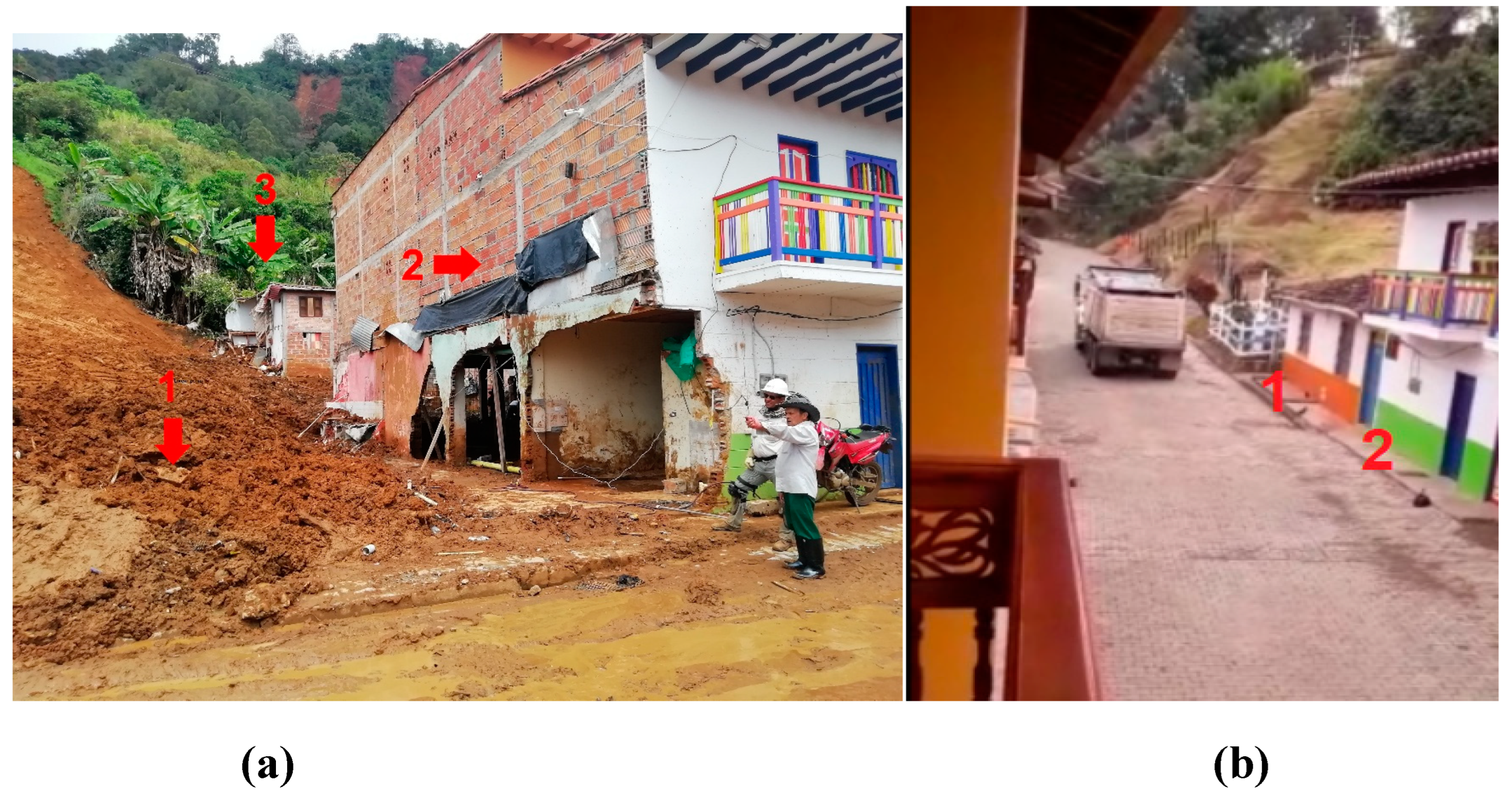
Figure 5.
(a) The reinforced first storey with reinforced concrete frames. Interior view. house 2; (b) Rear facade. House 2. Reinforced with reinforced concrete wall in the first storey.
Figure 5.
(a) The reinforced first storey with reinforced concrete frames. Interior view. house 2; (b) Rear facade. House 2. Reinforced with reinforced concrete wall in the first storey.
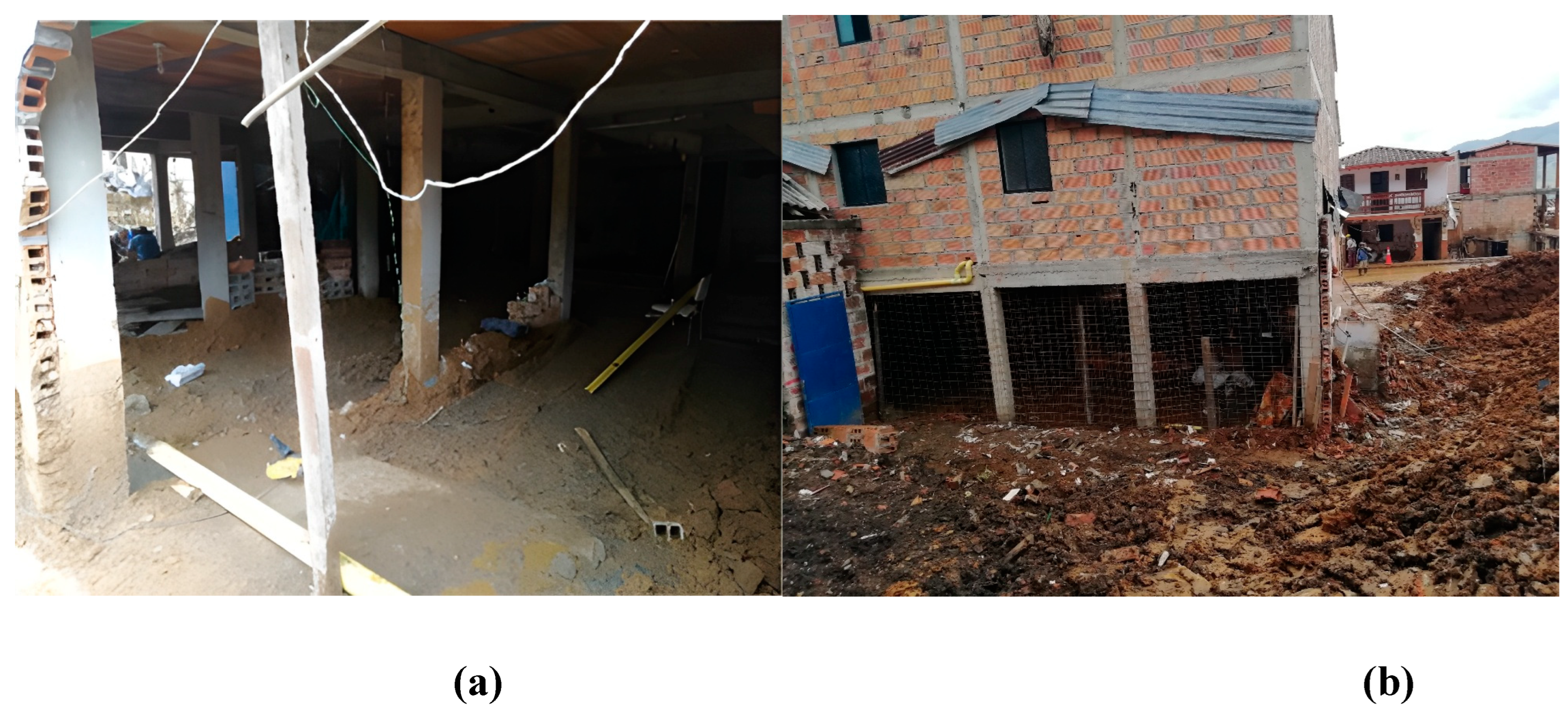
Figure 6.
(a) Side facade, infill walls total collapse, House 2; (b) Side facade. Infill walls without total collapse. House 2.
Figure 6.
(a) Side facade, infill walls total collapse, House 2; (b) Side facade. Infill walls without total collapse. House 2.
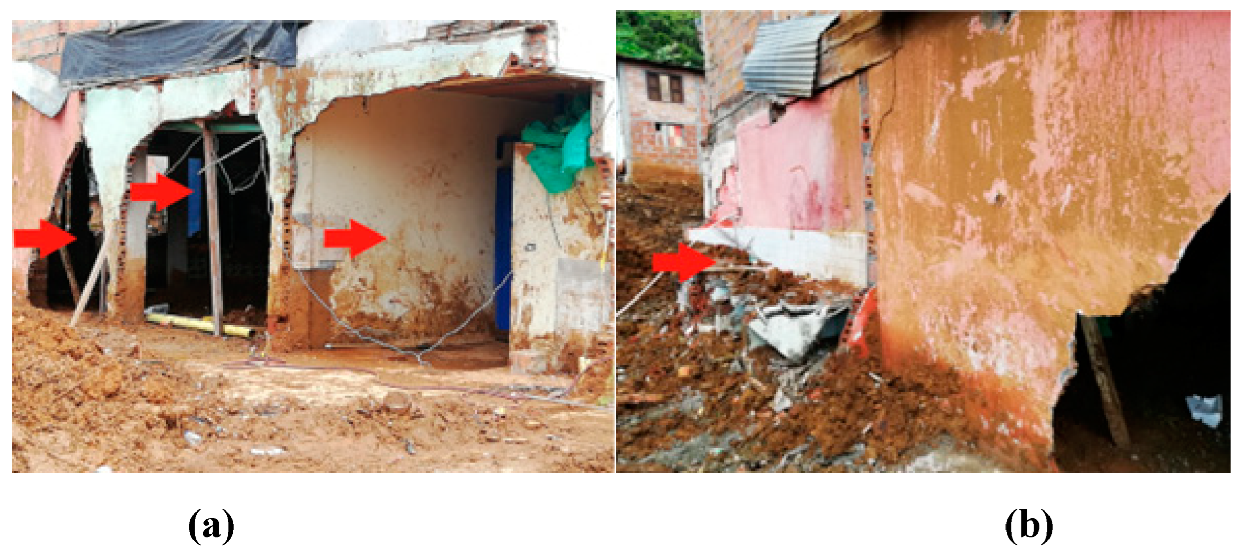
Figure 7.
(a) Partially confined masonry structure. Side facade. House 3; (b) Partially confined masonry structure. Front facade. House 3.
Figure 7.
(a) Partially confined masonry structure. Side facade. House 3; (b) Partially confined masonry structure. Front facade. House 3.
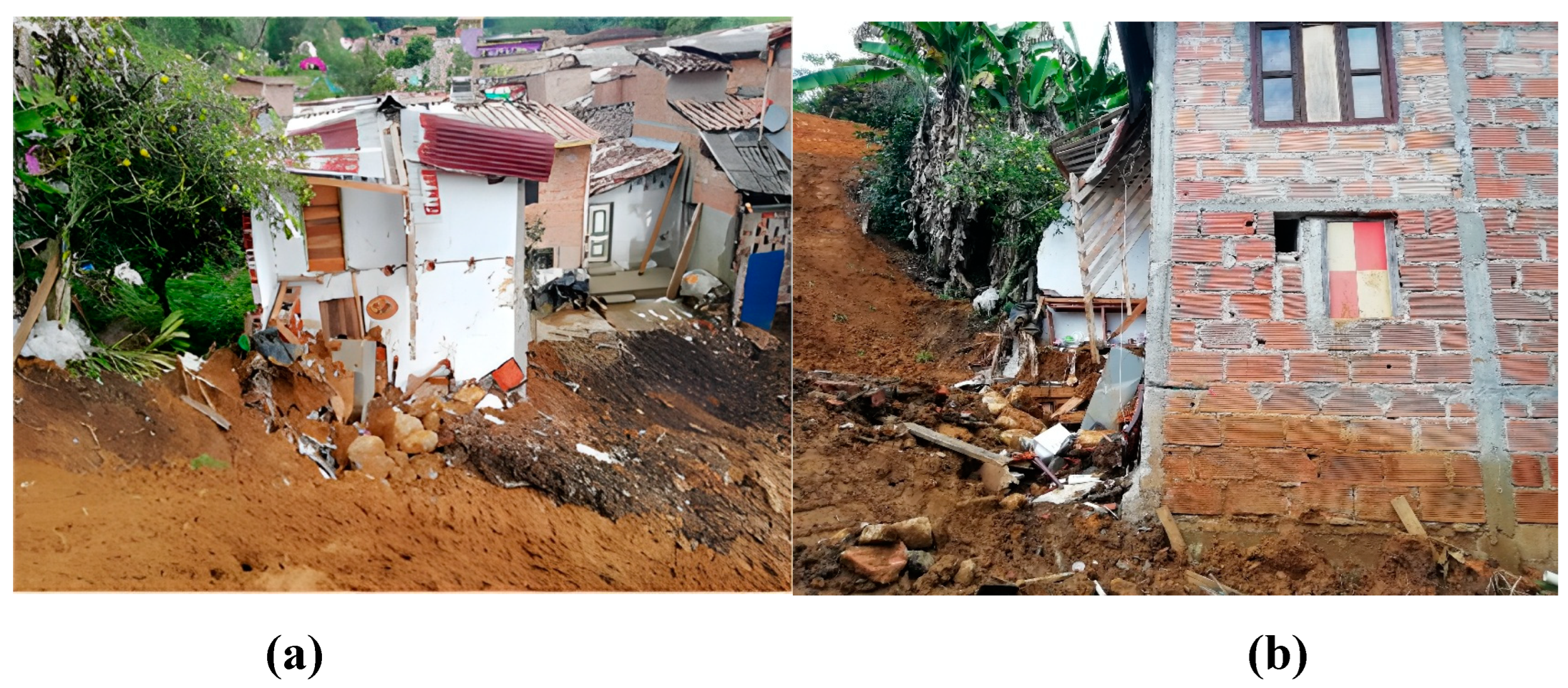
Figure 8.
(a) House 4 Collapsed by the landslide; (b) Debris from House 4 due to landslide.
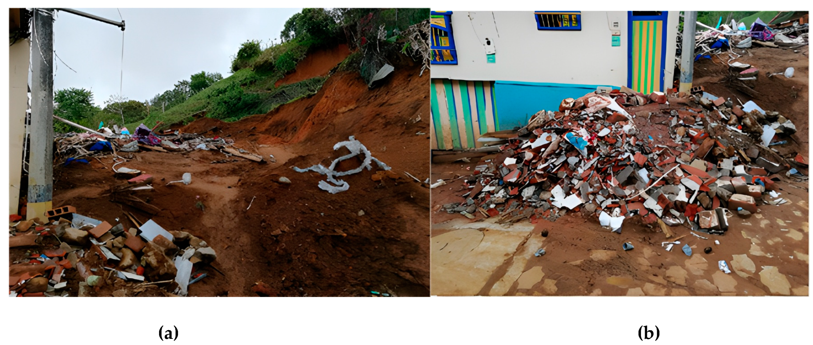
Figure 9.
(a) Building before the event. The image about 2nd Avenue. House 4. Source: Google Earth; (b) Building before the event. Image of the intersection of 2nd Avenue and 9th Street. House 4. Source: Google Earth.
Figure 9.
(a) Building before the event. The image about 2nd Avenue. House 4. Source: Google Earth; (b) Building before the event. Image of the intersection of 2nd Avenue and 9th Street. House 4. Source: Google Earth.
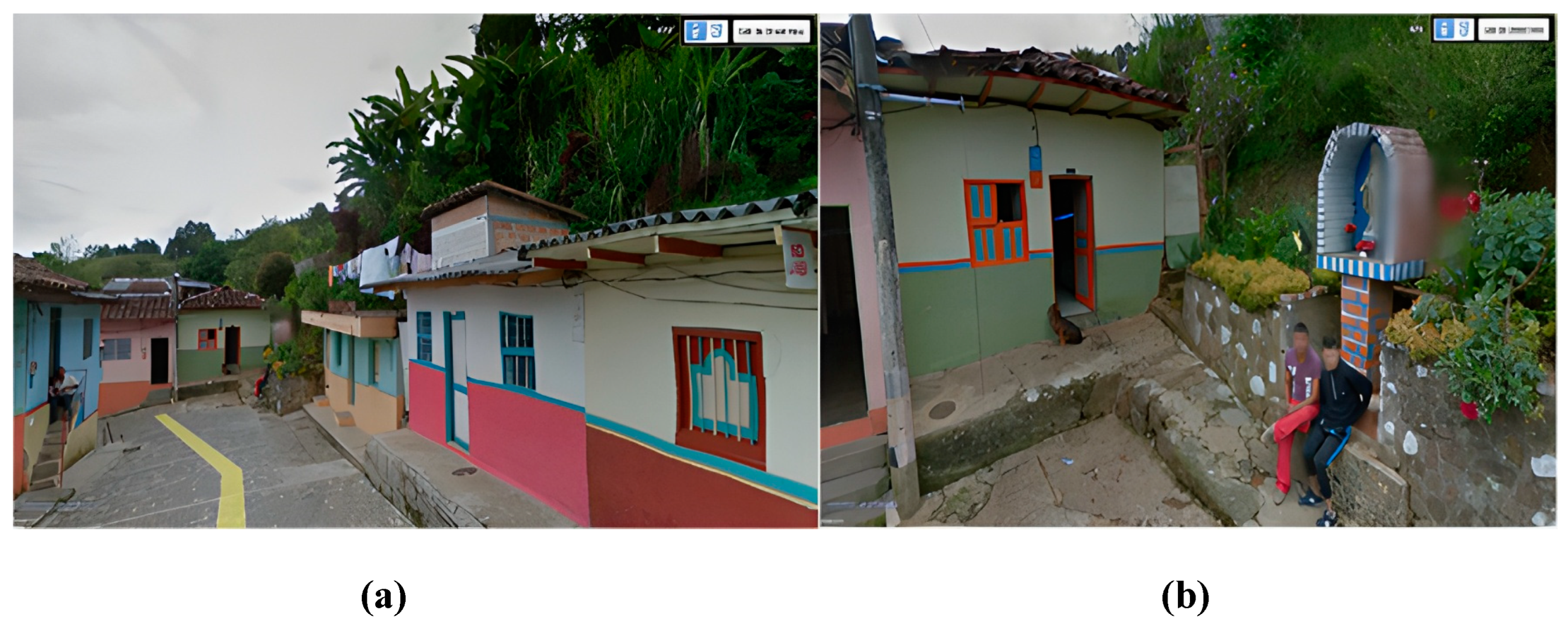
Figure 10.
(a) Affected building 1st Avenue – 7th Street, left side. House 5; (b) The facade affected, house 5, 1st Avenue – 7th Street, left side.
Figure 10.
(a) Affected building 1st Avenue – 7th Street, left side. House 5; (b) The facade affected, house 5, 1st Avenue – 7th Street, left side.
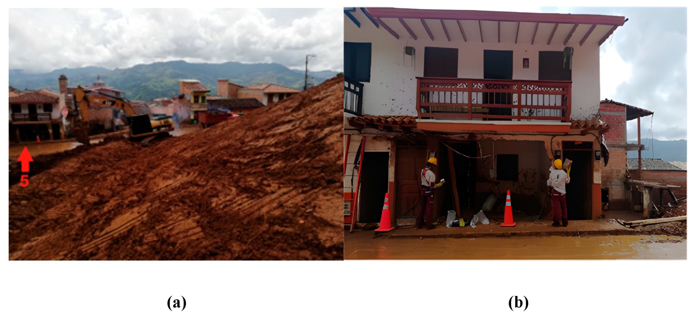
Figure 11.
(a) Affected buildings 1st Avenue – 7th Street, left side. Houses 5, 6 and 7; (b) Buildings original state 1st Avenue – 7th Street, left side. House 5, 6, and 7. Source: Google Earth.
Figure 11.
(a) Affected buildings 1st Avenue – 7th Street, left side. Houses 5, 6 and 7; (b) Buildings original state 1st Avenue – 7th Street, left side. House 5, 6, and 7. Source: Google Earth.
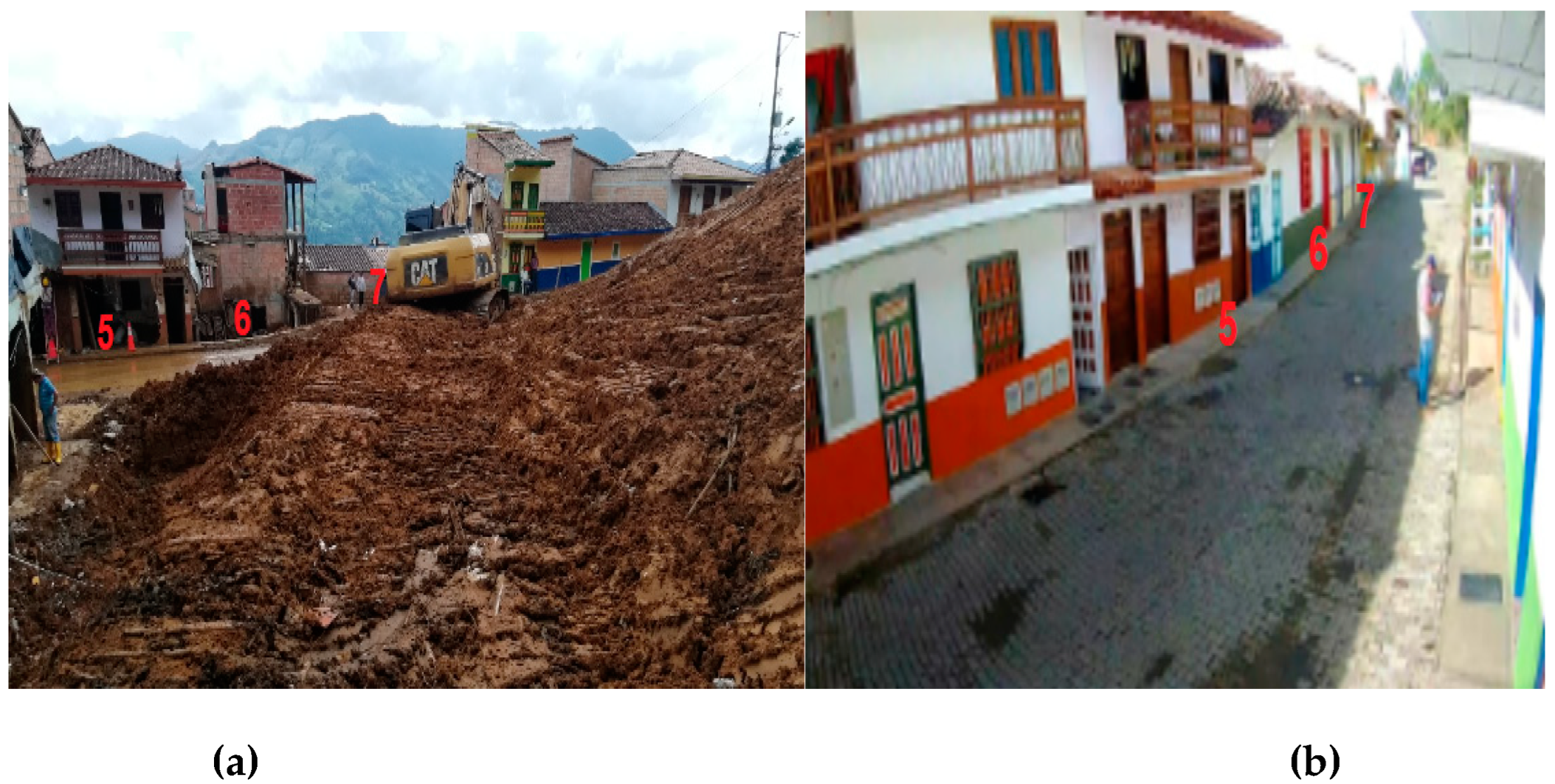
Figure 12.
(a) Houses 6 and 7 collapsed. Left side. 1st Avenue – 7th Street; (b) Affected building 1st Avenue – 7th Street, left side. house 6.
Figure 12.
(a) Houses 6 and 7 collapsed. Left side. 1st Avenue – 7th Street; (b) Affected building 1st Avenue – 7th Street, left side. house 6.
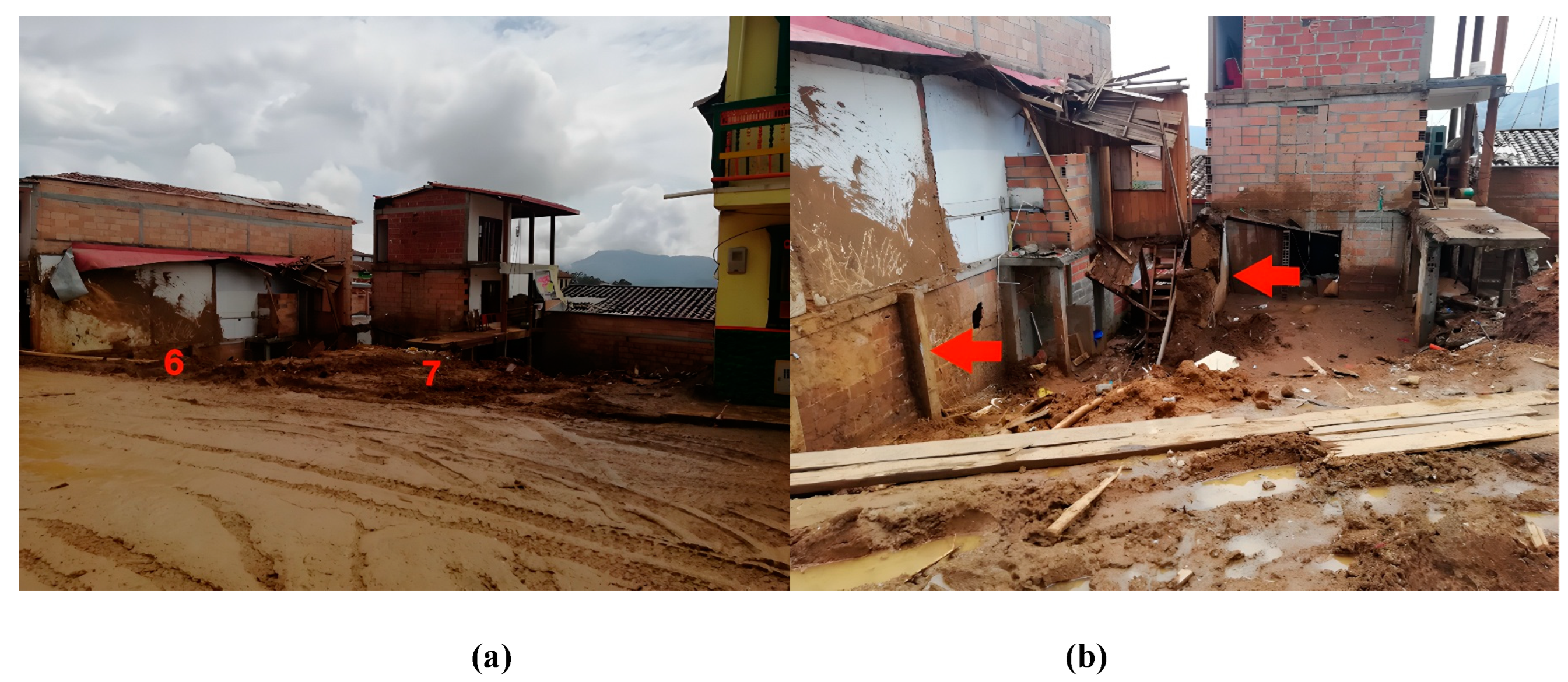
Figure 13.
(a) Affected building 1st Avenue – 7th Street, left side. House 6. Earth wall detail; (b) Affected building detail 1st Avenue – 7th Street, left side. house 6.
Figure 13.
(a) Affected building 1st Avenue – 7th Street, left side. House 6. Earth wall detail; (b) Affected building detail 1st Avenue – 7th Street, left side. house 6.
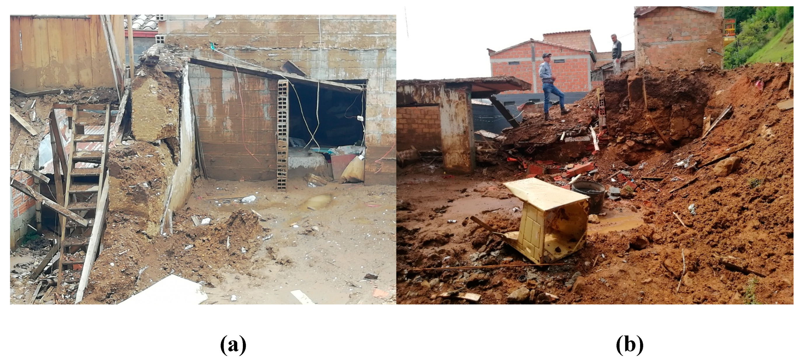
Figure 14.
(a) A power pole collapsed on 6th Street, lower slope of las Nubes Hill; (b) Collapsed power pole on 6th Street, lower slope of las Nubes Hill.
Figure 14.
(a) A power pole collapsed on 6th Street, lower slope of las Nubes Hill; (b) Collapsed power pole on 6th Street, lower slope of las Nubes Hill.
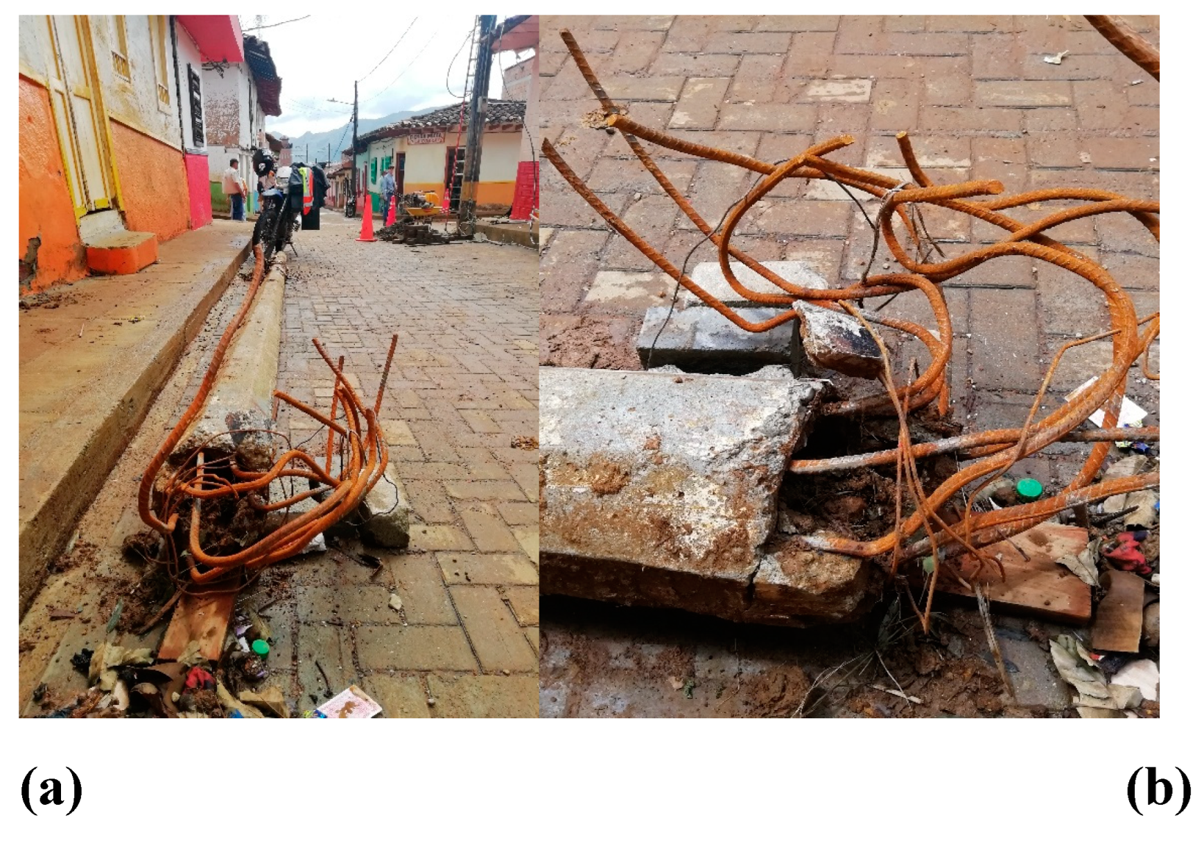
Figure 15.
(a) Architectural view of houses located on 6th Street and the lower part of the slope of Las Nubes Hill. Source: Google Earth; (b) View of affected houses on the hillside of las Nubes Hill, Valladares Stream, 6th Street. The photo was taken after evacuating the debris flow.
Figure 15.
(a) Architectural view of houses located on 6th Street and the lower part of the slope of Las Nubes Hill. Source: Google Earth; (b) View of affected houses on the hillside of las Nubes Hill, Valladares Stream, 6th Street. The photo was taken after evacuating the debris flow.
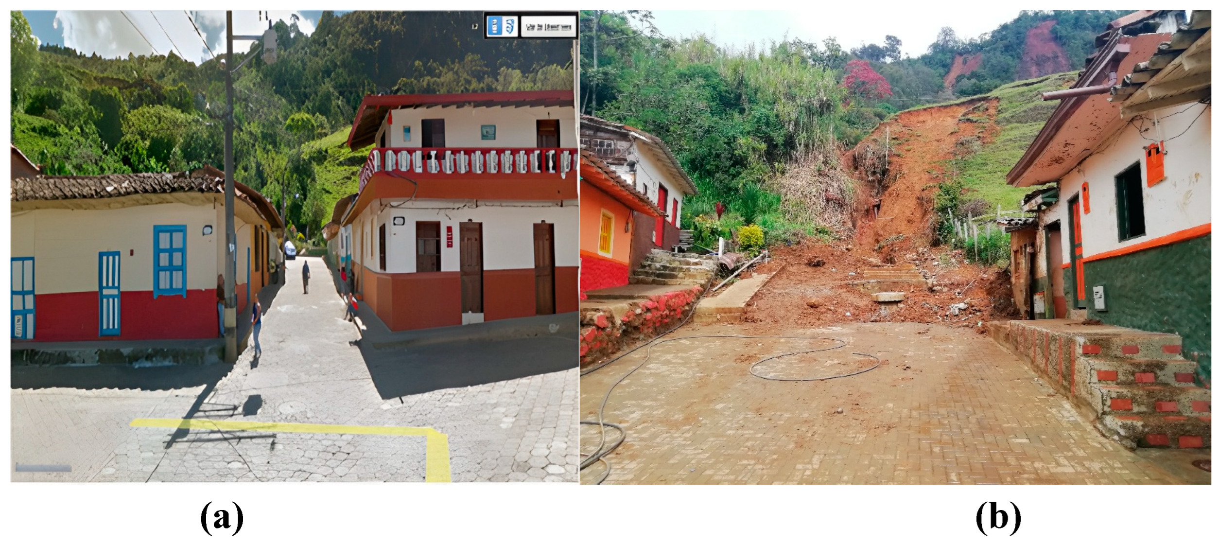
Figure 16.
(a) Affected houses on the hillside of Las Nubes Hill, Valladares stream. 6th Street; (b) Debris level measurement of houses affected hillside of Las Nubes Hill, Valladares stream. 6th Street. The photo was taken after evacuating the debris flow.
Figure 16.
(a) Affected houses on the hillside of Las Nubes Hill, Valladares stream. 6th Street; (b) Debris level measurement of houses affected hillside of Las Nubes Hill, Valladares stream. 6th Street. The photo was taken after evacuating the debris flow.
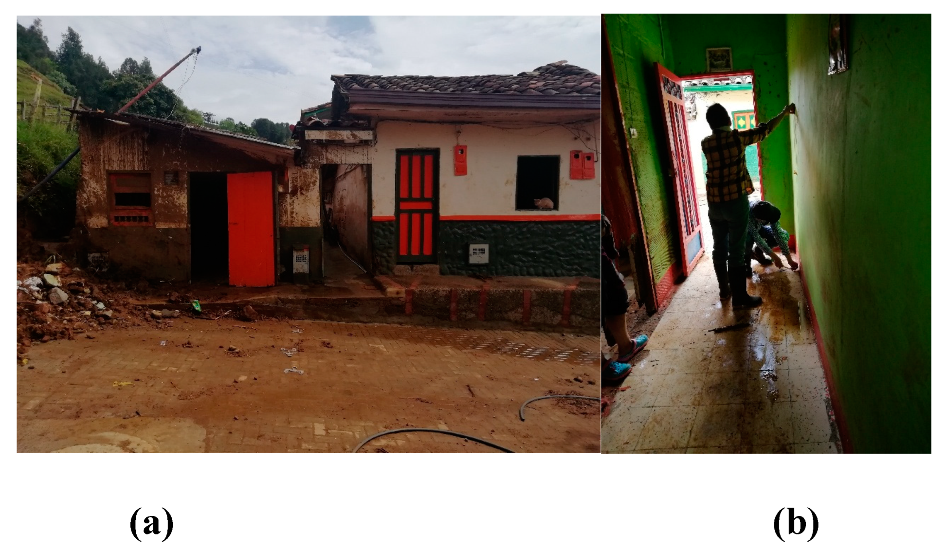
Figure 18.
Infill wall, subjected to dynamic lateral thrust due to landslide. 1st Avenue / 7th Street. Dwelling 2.
Figure 18.
Infill wall, subjected to dynamic lateral thrust due to landslide. 1st Avenue / 7th Street. Dwelling 2.
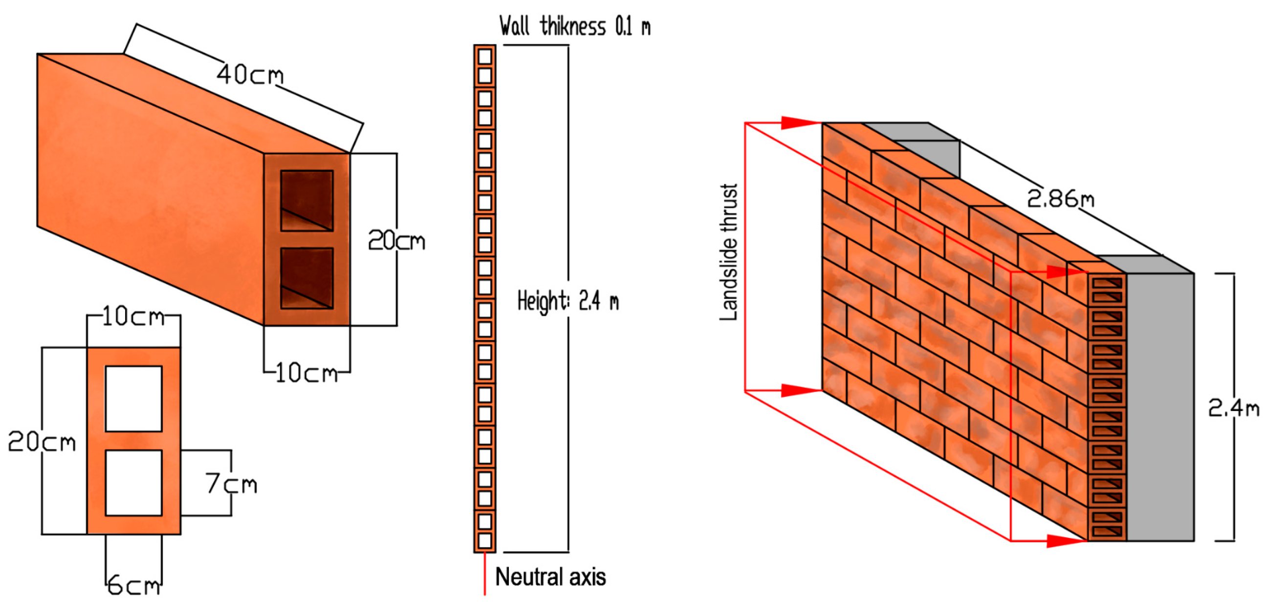
Figure 19.
Location of house 2 and landslide angle of attack. 1st Avenue, 7th Street.
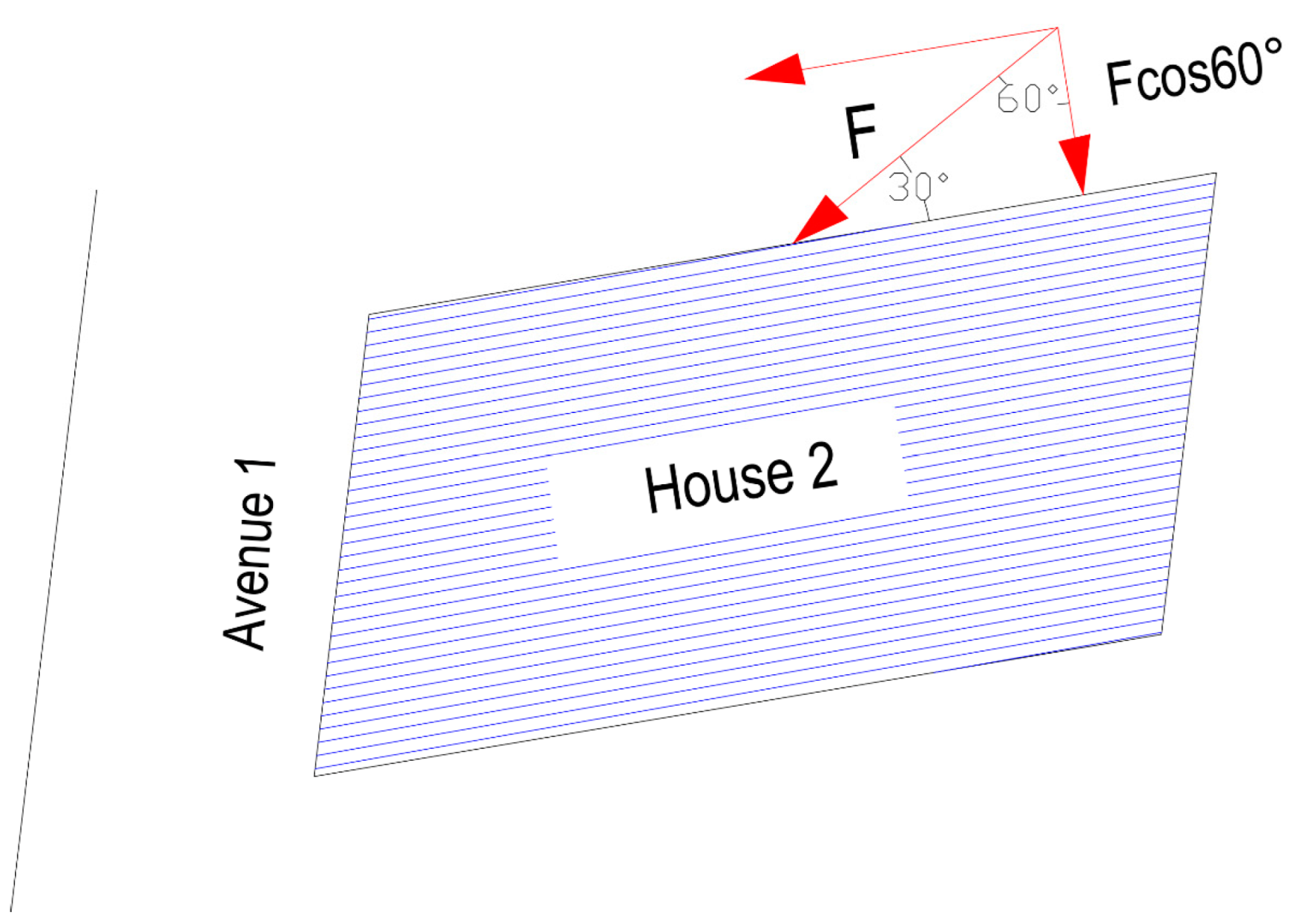
Figure 21.
Cross section of the power pole located on 6th Street on the slope of Las Nubes Hill.
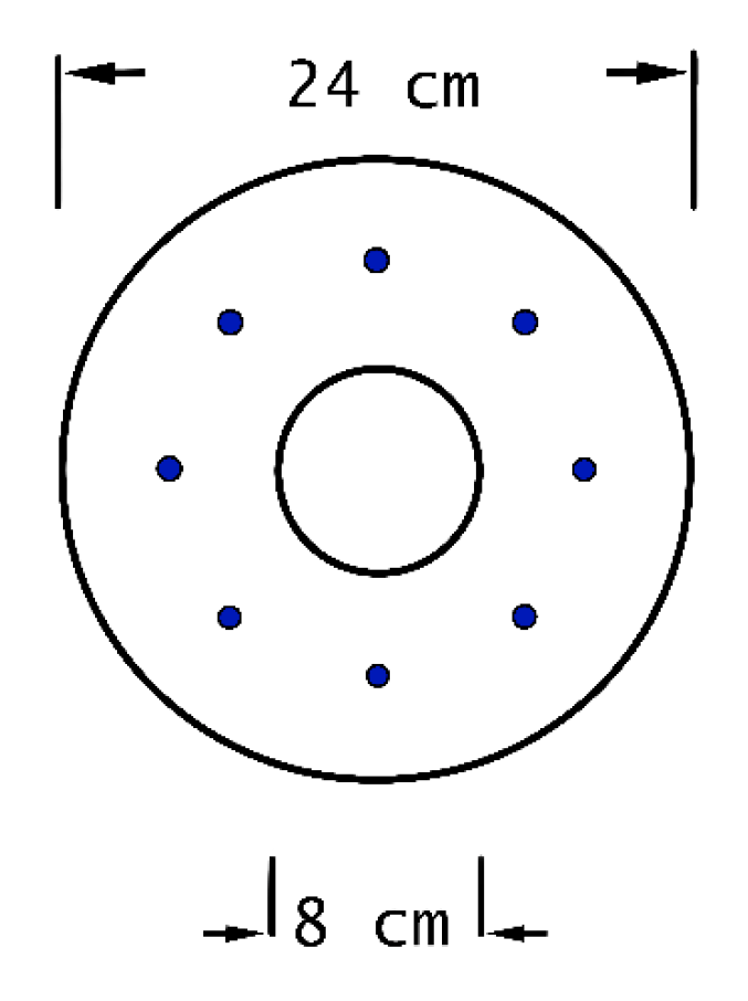
Table 5.
Mixed hydraulic models.
| Reference | Equation | |
| Arattano and Franzi (2003) | (38) | |
| Hübl and Holzinger (2003) | (19) | |
| Cui et al (2015) | (20) | |
| Gong, 2020 | (21) |
Table 6.
Field parameters for velocity calculation.
| Variable | Minimum | Maximum | Setting function |
| φ (˚) | 2.29 | 14 | uniform |
| β (˚) Houses 1, 6 y 7 | 14 | 15 | uniform |
| β (˚) House 4 | 16 | 17 | uniform |
| h' (m) Houses 1, 6 y 7 | 5 | 7 | uniform |
| h' (m) House 4 | 3 | 4 | uniform |
Table 7.
Statistical parameters for the calculation of velocity, houses 1, 6 and 7.
| Setting function | Triangular | |
| Minimum | 0.53 | |
| Maximum | 10.78 | |
| Mode | 9.15 | |
| Mean | 6.82 | |
| Median | 7.18 | |
| Standard deviation | 2.25 |
Note: Units are in m/s.
Table 8.
Statistical parameters for the calculation of velocity, house 4.
| Setting function | Pert | |
| Minimum | 1.75 | |
| Maximum | 8.32 | |
| Mode | 6.22 | |
| Mean | 5.83 | |
| Median | 5.92 | |
| Standard deviation | 1.21 |
Note: Units are in m/s.
Table 9.
Field parameters for dynamic thrust calculation.
| Input parameter | Minimum | Probable | Maximum | Median | Standard deviation | Setting function |
| v (m/s), Houses 1, 6 y 7 | 0.53 | 9.15 | 10.78 | Triangular | ||
| v (m/s), House 4 | 1.75 | 6.22 | 8.32 | Pert | ||
| h (m), Houses 6 y 7 | 1 | 2.5 | Uniform | |||
| h (m), House 4 | 1 | 2 | Uniform | |||
| B (m) | 6 | 8 | Uniform | |||
| ρ (kg/m3) | 1700 | 204.74 | Log normal | |||
| Kd | 1.2 | 0.67 | Log normal | |||
| Cd | 2 | 0.77 | Log normal |
Table 10.
Statistical parameters for dynamic thrust calculation.
| Event | Setting function | Mean | Median | Mode | Standard deviation |
| Houses 1, 6 y 7 | Lognormal | 1327 | 841.8 | 315.53 | 1622.9 |
| House 4 | Lognormal | 761 | 556.64 | 294.26 | 713.51 |
Note: Units are in kN.
Table 11.
Statistical parameters for momentum flux calculation (hv2).
| Setting function | General Beta (houses 1,6,7) | General Beta (houses 4) |
| α1 | 1.35 | 2.65 |
| α2 | 2.91 | 5.53 |
| Minimum | 0.56 | 4.3 |
| Maximum | 282.71 | 155.05 |
| Mean | 89.91 | 53.14 |
| Median | 81.26 | 50.89 |
| Mode | 44.15 | 44.56 |
| Standard deviation | 57.22 | 23.28 |
Note: Units are in m3/s2. α1 and α2 continuous shape parameters.
Table 12.
Field parameters, ultimate out-of-plane load capacity for infill walls by landslide.
| Input parameter | Minimum | Probable | Maximum | Median | Standard deviation | Setting function |
| f’m (MPa) | 3 | 0.9 | Log normal | |||
| H (m) | 2.3 | 2.6 | Uniform | |||
| B (m) | 2.7 | 2.9 | Uniform | |||
| t (m) | 0.1 | 0.12 | Uniform |
Table 13.
Statistical parameters, ultimate out-of-plane load capacity for infill walls by landslide.
Table 13.
Statistical parameters, ultimate out-of-plane load capacity for infill walls by landslide.
| Event | Setting function | Mean | Median | Mode | Standard deviation |
| House 2 | Lognormal | 11.3 | 10.75 | 9.72 | 3.73 |
Note: Units are in kN.
Table 14.
Field parameters, infill walls fragility curve due to out-of-plane loads by landslide, complete damage state.
Table 14.
Field parameters, infill walls fragility curve due to out-of-plane loads by landslide, complete damage state.
| Input parameter | Minimum | Probable | Maximum | Median | Standard deviation | Setting function |
| Fu (kN) | 10.75 | 3.73 | Log normal | |||
| Kd | 1.2 | 0.67 | Log normal | |||
| Cd | 2 | 0.77 | Log normal | |||
| ρ (kg/m3) | 1700 | 204.74 | Log normal | |||
| B (m) | 2.7 | 2.9 | Uniform |
Table 15.
Statistical parameters for the calculation of the infill walls fragility curve due to out-of-plane loads by landslide, complete damage state.
Table 15.
Statistical parameters for the calculation of the infill walls fragility curve due to out-of-plane loads by landslide, complete damage state.
| Event | Setting function | Mean | Median | Mode | Standard deviation |
| House 2 | Lognormal | 0.47 | 0.46 | 0.45 | 0.08 |
Note: Units are in m3/s2.
Table 16.
Parameters for calculating the debris flow velocity over 6th street coming from Las Nubes Hill.
Table 16.
Parameters for calculating the debris flow velocity over 6th street coming from Las Nubes Hill.
| Variable | Minimum | Maximum | Setting function |
| Cv | 0.1 | 0.9 | uniform |
| h (m) | 1.0 | 2.0 | uniform |
| p (%) | 2.0 | 14 | uniform |
| C | 0.0025 | 0.014 | uniform |
Table 17.
Statistical data for debris flow velocity calculation.
| Setting function | General Beta | |
| α1 | 16.80 | |
| α2 | 18.56 | |
| Minimum | 3.29 | |
| Maximum | 6.42 | |
| Mean | 4.78 | |
| Median | 4.78 | |
| Mode | 4.77 | |
| Standard deviation | 0.26 |
Note: Units are in m/s.
Table 18.
Field parameters for calculating debris flow dynamic thrust on the collapse of a power pole.
Table 18.
Field parameters for calculating debris flow dynamic thrust on the collapse of a power pole.
| Input parameter | α1 | α2 | Minimum | Maximum | Median | Standard deviation | Setting function |
| v (m/s) | 16.80 | 18.56 | 3.29 | 6.42 | General Beta | ||
| h (m) | 1.0 | 2.0 | Uniform | ||||
| ρ (kg/m3) | 1700 | 204.74 | Log normal | ||||
| Kd | 1.2 | 0.67 | Log normal | ||||
| Cd | 2 | 0.77 | Log normal |
Table 19.
Statistical data for calculating the debris flow dynamic thrust on the power pole.
| Setting function | Log normal | |
| Mean | 26.58 | |
| Median | 21.01 | |
| Mode | 13.14 | |
| Standard deviation | 20.58 |
Note: Units are in kN
Table 20.
Statistical data for calculating the power pole's debris flow momentum flux (hv2).
| Setting function | Pert | |
| Minimum | 17.04 | |
| Maximum | 59.93 | |
| Mean | 34.46 | |
| Median | 33.98 | |
| Mode | 32.44 | |
| Standard deviation | 7.96 |
Note: Units are in m3/s2.
Table 21.
Statistical data for calculating the debris flow overturning moment (h2 v2).
| Setting function | Pert | |
| Minimum | 17.71 | |
| Maximum | 119.16 | |
| Mean | 53.41 | |
| Median | 51.09 | |
| Mode | 41.96 | |
| Standard deviation | 20.43 |
Note: Units are in m4/s2.
Table 22.
Field parameters, ultimate power pole load capacity.
| Input parameter | Minimum | Probable | Maximum | Median | Standard deviation | Setting function |
| f’c (MPa) | 14 | 4 | Log normal | |||
| De (m) | 0.2 | 0.21 | Uniform | |||
| Di (m) | 0.06 | 0.08 | Uniform |
Table 23.
Statistical parameters, ultimate power pole load capacity.
| Event | Setting function | Mean | Median | Mode | Standard deviation |
| Power pole | Lognormal | 18.33 | 18.13 | 17.75 | 2.66 |
Note: Units are in kN
Table 24.
Field parameters, power pole complete damage threshold due to momentum flux.
| Input parameter | Minimum | Probable | Maximum | Median | Standard deviation | Setting function |
| Fu (kN) | 18.13 | 2.66 | Log normal | |||
| Kd | 1.2 | 0.67 | Log normal | |||
| Cd | 2 | 0.77 | Log normal | |||
| ρ (kg/m3) | 1700 | 204.74 | Log normal | |||
| B (m) | 0.375 | 0.375 | Uniform |
Table 25.
Statistical parameters, power pole complete damage threshold due to momentum flux.
| Event | Setting function | Mean | Median | Mode | Standard deviation |
| Power pole | Lognormal | 36.15 | 28.87 | 17.54 | 26.31 |
Note: Units are in m3/s2.
Table 26.
Field parameters, power pole complete damage threshold due to overturning moment.
| Input parameter | Minimum | Probable | Maximum | Median | Standard deviation | Setting function |
| fy (MPa) | 240 | 15 | Log normal | |||
| Kd | 1.2 | 0.67 | Log normal | |||
| Cd | 2 | 0.77 | Log normal | |||
| ρ (kg/m3) | 1700 | 204.74 | Log normal | |||
| B (m) | 0.375 | 0.375 | Uniform | |||
| As (cm2) | 3 | 5 | Uniform |
Table 27.
Statistical parameters, power pole complete damage threshold due to overturning moment.
| Event | Setting function | Mean | Median | Mode | Standard deviation |
| Power pole | Lognormal | 70.79 | 56.46 | 35.91 | 53.55 |
Note: Units are in m4/s2.
Disclaimer/Publisher’s Note: The statements, opinions and data contained in all publications are solely those of the individual author(s) and contributor(s) and not of MDPI and/or the editor(s). MDPI and/or the editor(s) disclaim responsibility for any injury to people or property resulting from any ideas, methods, instructions or products referred to in the content. |
© 2025 by the authors. Licensee MDPI, Basel, Switzerland. This article is an open access article distributed under the terms and conditions of the Creative Commons Attribution (CC BY) license (http://creativecommons.org/licenses/by/4.0/).
Copyright: This open access article is published under a Creative Commons CC BY 4.0 license, which permit the free download, distribution, and reuse, provided that the author and preprint are cited in any reuse.


