
Submitted:
22 February 2025
Posted:
24 February 2025
You are already at the latest version
Abstract
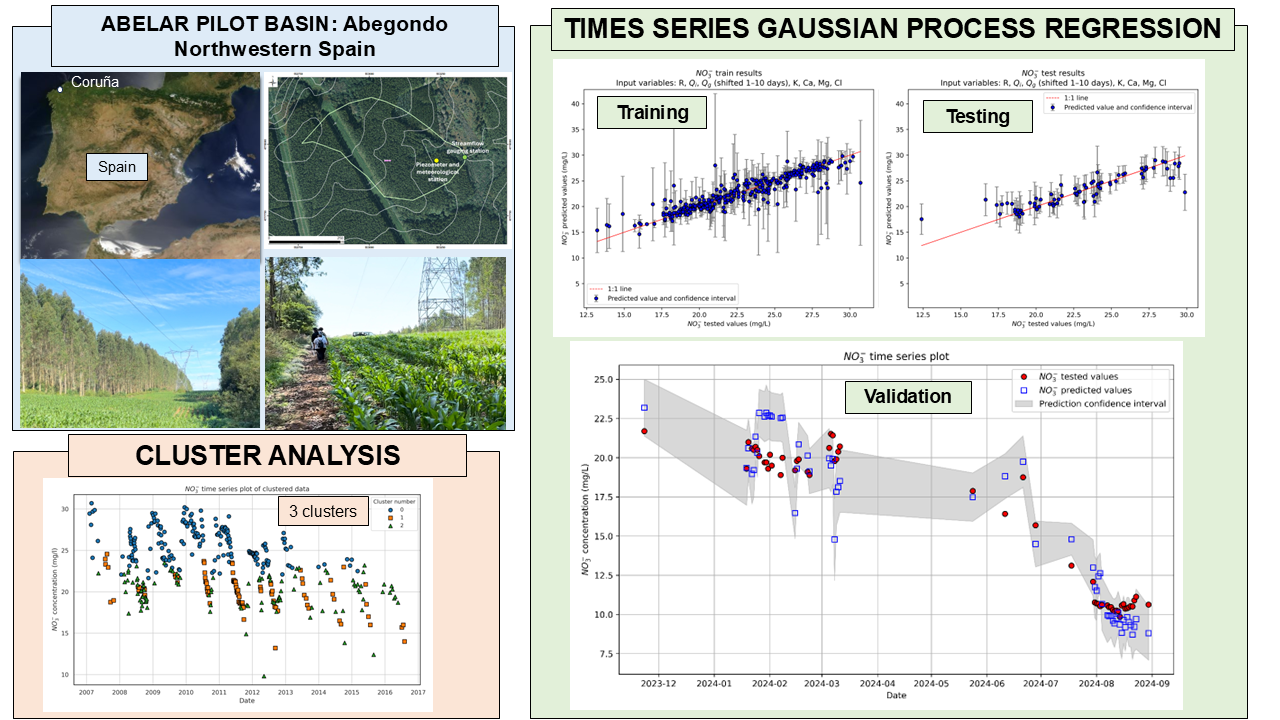
The Abelar pilot basin in Coruña (Northwestern Spain) has been monitored for hydrological and hydrochemical data to assess the effects of eucalyptus plantation and manure applications on water resources, water quality and nitrate contamination. Here we report the machine learning analysis of hydrological and hydrochemical data from the Abelar basin. K-means Cluster Analysis (CA) is used to relate nitrate concentrations at the outlet of the basin with daily interflows and groundwater flows calculated with a hydrological balance. CA identifies three linearly separable clusters. Times Series Gaussian Process Regression (TS-GPR) is employed to predict surface water nitrate concentration by incorporating hydrological variables as additional input parameters using a time series shifting. TS-GPR allows modeling nitrate concentrations based on shifted interflows and groundwater flows and chemical concentrations with R2 = 0.82 and 0.80 for training and testing, respectively. Groundwater flow from five days prior to the current date, Qg5, is the most important input parameter of the TS-GPR model. Interaction effects between the variables are found. TS-GPR validation with recent data provides results consistent with those of testing (R2 = 0.85). Model inspection by permutation feature importance and partial dependence plots shows interactions between Qg5 and Cl, and between Ca and Mg.
Keywords:
K-means clustering
; Gaussian Process Regression
; time series analysis
; Abelar pilot basin
; nitrate concentration
; applied machine learning
; hydrological data
; hydrochemical data
1. Introduction
In the last two decades, machine learning (ML) has emerged as a transformative tool for analyzing complex and high-dimensional hydrological and hydrochemical datasets, offering novel insights and predictive capabilities. Datasets are often high-dimensional, with temporal and spatial variability posing significant challenges. Common ML techniques for analyzing river streamflow and water quality data include: 1) Supervised Learning with algorithms such as Artificial Neural Networks (ANNs), Random Forests, Support Vector Machines, and Gradient Boosted Trees are widely used for classification and regression tasks; 2) Deep Learning: Recurrent Neural Networks (RNNs) and Long Short-Term Memory (LSTM) networks are effective for time-series prediction, while Convolutional Neural Networks (CNNs) are applied to spatial pattern recognition; 3) Unsupervised Learning such as Clustering methods, dimensionality reduction techniques Principal Component Analysis (PCA), and T-distributed Stochastic Neighbour Embedding (t-SNE) assist in identifying patterns and anomalies in water quality data; and 4) Hybrid Models, which integrate ML with traditional hydrological models such as SWAT and MODFLOW), have improved the prediction accuracy and the interpretation of model results. A notable advancement in this category is Physics-Informed Neural Networks (PINNs), which embed governing physical equations within deep learning frameworks to jointly estimate parameters and states, making them particularly effective for subsurface transport and sparse-data scenarios.
ANNs have been used to estimate nitrate concentrations in groundwater based on in-situ field data, with results demonstrating that incorporating land use variables significantly improved model performance in terms of Root Mean Squared Error (RMSE) offering a promising tool for managing groundwater contamination in the Asopos River Basin and Kopaidian Plain, Greece [1]. Random Forests were compared with linear modeling to estimate the concentration of nutrients including nitrate in a rural catchment, using commonly measured in-situ variables as surrogates, leading to a reduction in RMSE of up to 60.1% [2]. Random Forests outperformed other ML models in predicting total nitrogen concentrations in inland rivers with 92.94% accuracy and were also used to model salinity using remote sensing data. Support Vector Machines and Gradient Boosting effectively predicted water quality indicators, such as turbidity and nutrient levels, across diverse watersheds [3]. Random Forest regression was found to provide accurate predictive models for nitrate pollution in groundwater, identifying key predictors of pollution, and outperforming logistic regression in generating vulnerability maps for water resources management [4].
LTSM networks effectively modelled complex, non-linear, and temporal dependencies in hydrological data, outperforming traditional models in streamflow prediction, particularly under high variability, and offering improved predictive capabilities and potential for real-time hydrological forecasting [5]. A LSTM model was also used to predict river dissolved oxygen dynamics, effectively capturing its relationship with water temperature across 236 U.S. watersheds and highlighting the potential of deep learning models for predicting river water quality at large scales [6]. Standalone LSTM and CNN models, along with a coupled CNN-LSTM model, were developed to predict water quality variables—dissolved oxygen (DO) and chlorophyll-a (Chl-a)—in Small Prespa Lake, Greece, using time-series data of physicochemical variables. The coupled CNN-LSTM model outperforms both standalone and traditional ML models, demonstrating its ability to capture both low and high levels of water quality variables. LSTM performs the best for DO prediction [7].
Hierarchical Cluster Analysis (HCA) was used to analyze hydrochemical datasets, comparing different linkage methods to optimize classification for complex hydrological systems [8]. HCA and Mahalanobis distance metrics were employed to monitor human-induced changes in the Jinjiang River's hydrochemistry, highlighting pollution impacts from agriculture and mining [9]. t-SNE was introduced as a graphic approach to assist HCA in groundwater geochemistry, outperforming PCA in determining the number of clusters and delineating spatial geochemical zones. However, t-SNE reliance on hyperparameter tuning limits its standalone use [10]. A hybrid model approach combining LSTM networks with the SWAT model was proposed to improve streamflow prediction, demonstrating the benefits of integrating ML with traditional hydrological models for more accurate and interpretable predictions [11]. Previous studies have focused on the use of K-means clustering to provide information on processes affecting aquifers [12,13]. A multiphysics-informed deep neural network approach based on PINNs was proposed for estimating space-dependent hydraulic conductivity, hydraulic head, and concentration fields from sparse measurements by jointly training deep neural networks with governing equation residuals, demonstrating superior accuracy over standard data-driven methods, particularly in sparse data scenarios [14].
Regression models have been used very scarcely in the field of groundwater quality, and mainly through linear regression and multiple linear regression methods as the benchmark for the lowest acceptable accuracy [15]. Gaussian Process Regression (GPR) was found to be an effective tool in predicting nitrate concentration in groundwater based only on water quality chemical input parameters, outperforming popular Decision Tree algorithms [16]. Similarly, GPR consistently yielded good performance in predicting surface water nitrate concentration across various watersheds with differing land-use practices, including agriculture and forest land-use, using streamflow as the only input parameter [17].
The water supply of the population in Atlantic European regions living in dispersed rural areas is managed privately through autonomous solutions, such as domestic wells or neighbourhood water systems that capture springs. There is growing concern about microbiological and nitrate contamination of groundwater. This contamination is caused by the improper management of organic fertilizers in agriculture, slurry discharges from farms, and land-use planning that does not consider water sources [18,19]. Implementing European regulations on drinking water (Directive 98/83/EC) and water protection and management (Directive 2000/60/EC) in these communities poses a significant challenge for water administration, as the feasibility of centralized infrastructure is limited by the enormous investments required and the high maintenance costs. More than 50% of the population of Abegondo (A Coruña, Spain) relies on autonomous water systems [19]. The main issues for the sustainability of these systems include: (1) Insufficient supply reliability; (2) Deterioration of water quality; and (3) Deficiencies in the governance of groundwater use and waste management [20]. [18] presented the results of a hydrogeological study that analyzed the vulnerability of groundwater to contamination and the protection of water sources in rural areas of Abegondo (A Coruña). Subsequently, [20] presented an analysis of the sustainability of autonomous groundwater supply systems in the rural areas of Abegondo, which are located in fractured hard rocks. There is a concern about the chemical and microbiological quality of groundwater supply in rural areas due to the lack of proper control of the water quality by well owners. Agricultural contamination is often a pressure on the groundwater chemical status where nitrate is the main concern for groundwater quality.
Hydrological research and water resources assessment were performed in the Abelar pilot watershed in Abegondo by [21] and [21] (Figure 1). This small watershed has a surface area of about 10.7 ha. It was equipped with two meteorological stations, two piezometers and a streamflow gauging station [20,21]. The results show that fast-growing trees with high water consumption can reduce the availability of water resources, especially in the summer months and other dry periods, which can be manifested in the decrease in piezometric levels and the eventual drying up of springs and riverbeds. A hydrometeorological water balance model of the Abelar site was presented by [20] to quantify the water resources in this basin planted with eucalyptus. The hydrological model of the Abelar basin was calibrated with piezometric and streamflow data [20].
Here we present the machine learning analysis of hydrological and hydrochemical data from the Abelar basin. K-means clustering is used to identify groups for nitrate concentration and hydrological flows (interflow and groundwater flow). Our work also further explores the underrepresented regression model of GPR, extending its scope to predict surface water nitrate concentration by incorporating hydrological variables as additional input parameters using a time series shifting approach. Specifically, the methods of Cluster Analysis (CA) and GPR for Time Series (TS-GPR) are applied to group and predict surface water nitrate concentration. The paper starts with the description of the Abelar pilot basin, the available data, and the ML methods used. Then, model results are presented for the ML methods. Afterwards, a discussion of the main findings is presented. The paper ends with the main conclusions and future work suggestions to improve the individual performance of the ML methods as well as their potential coupling.
2. Materials and Methods
2.1. Abelar pilot basin and available data
The Abelar pilot basin has been monitored for hydrological and hydrochemical data during the last decades. These data have been used to assess the effects of eucalyptus plantation on water resources, soil properties, water quality and nitrate contamination due to excessive manure applications. The Abelar basin is located at the catchment of the Tambre river basin (Figure 1). The average elevation of the basin is 413 m above sea level. The climate is humid and oceanic with relatively abundant rainfall. The mean annual precipitation in the period 1997 - 2016 is equal to 1577 mm. Temperatures are mild and show little oscillation between maximum and minimum (16.7 ºC in summer and 8.1ºC in winter). November and December are the rainiest months. The climate of the study area is of the Csb type according to the Köppen-Geiger classification [23]. The basin is located on schists (metapsamites and metapelites) of the Betanzos Unit. The weathering and alteration of shale gives rise to a surface layer of variable thickness between 1 and 2 m, in some cases reaching 5 m [19]. The vegetation consists of Eucalyptus globulus and low shrubs. Groundwater recharge occurs mainly due to the infiltration of rainwater. The discharge of diffuse or localized groundwater flow occurs in the valleys and low areas of the basin. The basin of the farm has been characterized continuously since the hydrological year 1997/98 in which the plantation was carried out and an automatic and a manual weather station, an automatic streamflow gauging station and two piezometers were installed.
The characterization of the main creek in the Abelar pilot basin at the in-situ automatic streamflow gauging station has produced a wealth of hydrochemical data since its installation. The focus of this study is on analyzing the combination of such surface water hydrochemical data with meteorological data and hydrological model outputs such as daily groundwater recharge rates, interflows and groundwater flows [19]. The Abelar dataset contains data on hydrological and hydrochemical properties of the Abelar basin in Abegondo, La Coruña (Spain). The specific attributes of the Abelar dataset given are listed in Table 1. The dataset contains 9679 entries of daily meteorological, hydrological and hydrochemical data corresponding to the period from October 1, 1997, to March 31, 2024. While meteorological and hydrological data are available every day, the hydrochemical data are available at some specific dates corresponding to the water sampling dates from January 26, 2007, to July 30, 2024. The number of data is 403 for all species except for: Fe (401 observations), Cu (393 observations), Zn (397 observations), Al (398 observations) and Vn (394 observations). Subsequently, additional hydrochemical data up to August 30, 2024, were obtained and the simulated hydrological data extended accordingly. Simulations of hydrological data were performed with the code VISUAL BALAN v2.0 (e.g., [24,25,26]), which is based on a semi-distributed model that performs daily water balances in the soil, the underlying unsaturated zone and the aquifer. VISUAL BALAN evolved from earlier versions of the code which had the generic name of BALAN [24,27]. The hydrological components are evaluated daily in a sequential manner. The daily values of precipitation and streamflow components are shown in Figure 2.
Figure 3 shows the temporal evolution of concentration data. These data are grouped based on the following three conditions: 1) Predominant interflow with interflow being greater than 75% of the total flow; 2) Predominant groundwater flow with groundwater being more than 80% of the total flow; and 3) Interflow fraction ranging from 20% to 75%. Nitrate, chloride, calcium, magnesium and potassium concentrations at the basin outlet were collected from January 2007 to December 2015. The second sampling campaign started in the spring of 2023 and includes data until November 2024. Nitrate concentrations range from 10 to 40 mg/L, with two peaks of 150 mg/L. Nitrate concentrations fluctuate in response to hydrological variations in the basin. Higher nitrate concentrations are associated with an increase in interflow, while lower concentrations correspond to larger groundwater flows. The lowest nitrate concentrations, typically observed during the dry (low flow) season, are considered more representative of groundwater concentrations. Chloride, calcium, magnesium, and potassium concentrations exhibit trends like nitrate, although with less pronounced variations.
2.2. ML methods
The following methods were used for the selected hydrochemical target variables such as nitrate concentration: 1) Cluster Analysis (CA) and 2) Time Series Gaussian Process Regression (TS-GPR). Data preprocessing was performed for both methods prior to modelling, as required by ML techniques.
2.2.1. Data preprocessing
Data preparation was conducted by following two slightly different processes for CA and TS-GPR ahead of modelling.
The data preprocessing before the CA included data exploration through histograms, heatmaps and pair plots of the data to look for correlation among variables. Feature engineering was conducted prior to the K-means modeling, including the log-transformation of all input variables. This transformation involved applying the natural logarithm to one plus the variable's value to account for values equal to or near zero. Log-transforming the input variables helped address their skewed distributions. Notably, the target variable (nitrate) was not subjected to log-transformation.
The data preparation for TS-GPR began with resampling the data to a daily frequency to account for the irregular frequency of sampling of chemical data. Days with several chemical samplings were resampled by taking the mean value of the observations for each date. Anomalous values were identified and removed from the data using the Quantile-Based Outlier Detection (QBOD) method. QBOD is a technique that utilizes statistical quantiles to detect outliers by comparing each data point to a range defined by quantiles. It extends the interquartile range (IQR) analysis introduced by [28], incorporating flexible quantile-based thresholds to make it more robust to skewed distributions. The number of anomalous values was defined by setting lower and upper quantile bounds. Preliminary analyses determined that using quantiles of 0.25 and 0.75 provided the best balance between retaining informative data and excluding extreme anomalous data that could skew the model results. Four anomalous samples were identified and removed from nitrate data, corresponding to the top four values in the distribution.
2.2.2. Cluster Analysis
Cluster analysis involves classifying an integrated hydrological system (defined as the combination of hydrological and hydrochemical data) into sub-hydrological systems based on the ratio of interflow to total flow (), the ratio of groundwater flow to total flow () and nitrate concentration. The clustering K-means algorithm implemented in the Scikit-learn package 1.5.2 of the Python programming language was used in this approach [29]. The unsupervised K-means algorithm [30] is an iterative process in which similar observations are grouped together. The algorithm starts by taking two random points known as centroids and continues by calculating the distance of each observation to the centroid and assigning each cluster to the nearest centroid. After the first iteration, every point belongs to a cluster. Next, the number of centroids increases by one, and the centroid for each cluster is recalculated as the points with the average distance to all points in a given cluster. The process is repeated k-times until no observation is assigned to another cluster. The algorithm converges when clusters do not move anymore.
CA for the groups was carried out by fitting twenty K-means models on the data with values of the cluster number ranging from 1 to 20 and storing for each model the number of clusters and the inertia value. The resulting dataset after data preprocessing consisted of 388 samples (after removing four anomalous values), all of which were used for training. The input variables or features for the K-means models were , and nitrate concentration. The optimal number of clusters was then visually determined based on the plot of inertia versus the number of clusters (elbow method). The final clusters were both visualized with pair plots and statistically analyzed. The methodology for the CA model applied in this study is outlined in Figure 4.
The main advantage of the K-means algorithm is that it is easy to compute. A disadvantage is that this algorithm is sensitive to the choice of the initial points, so different initial configurations may yield different results. To resolve this, a more intelligent initialization method for K-means clusters, known as K-means ++, helps avoid falling into local optima. This is the default implementation of the K-means in Scikit-learn which was used here.
2.2.3. Times Series Gaussian Process
Gaussian Process (GP) is a nonparametric supervised learning method commonly used to solve regression and probabilistic classification problems [31]. GP is an exact interpolator for noise-free data and regular covariance functions (kernels). GP predictions are probabilistic and therefore GP allows for computing approximate confidence intervals. The Gaussian Process algorithm aims at estimating a real-valued function, defined on a compact subset by using a finite set of data values, , corresponding to locations with i = 1, 2, … t, where t is the number of training data points and d is the dimensionality of function . It is assumed that is a GP having a covariance function ) which quantifies the covariance of at locations and . GP provides unbiased and minimum variance estimates of conditioned on the training data set of observations. The posterior distribution of the GP has a mean and a covariance function which are given by:
where and are column vectors of the locations of the t query or testing points, and in the input domain where the GP algorithm predicts the values of or computes the covariance matrix which has entries ) with i,j = 1, 2, … t. is the covariance of the estimates of at locations and and and are -dimensional column vectors given by and , respectively and T denotes the vector/matrix transpose. For further details on GP, we refer the reader to [31] which presents thoroughly the properties of GP.
A kernel is a crucial ingredient of GP which determines the shape of the prior and posterior distributions of the GP. The covariance) of a stationary GP depends only on the Euclidian distance d between the two points and . Here we used the Matérn stationary kernel which is a generalization of the radial basis function kernel [32] and is given by:
where is a modified Bessel function and is the gamma function. l (>0) is a length-scale parameter and v is a parameter controlling the smoothness of the kernel covariance function.
In the system considered here, models a physical quantity, e.g. species concentration, that is assumed to be smooth and is either the squared exponential covariance function or the Matérn covariance function, both commonly used in this case.
The method of TS-GPR implements a Gaussian Process regressor approach that models temporal dependencies by defining a kernel over sequential data, enabling complex pattern recognition and uncertainty quantification over time. The Gaussian Process Regression (GPR) algorithm implemented in the Scikit-learn package 1.5.2 was used in this study. Sequential data for time series were generated through data shifting, a feature engineering technique that creates lagged features from the available data to model temporal dependencies. Hence, once the target variable was selected, the hydrological variables of the dataset were shifted, using time lags up to 10 days, while the hydrochemical variables were kept fixed at the same date as that of the observations of the target variable. Using a time lag of 1 day is equivalent to keeping the parameters fixed. As a result of data shifting, a dataset of shape m × n was generated, where m is the number of days on which both hydrological and hydrochemical data are available, and n represents the number of total variables after shifting, including the target variable.
Only data up to the year 2016 were used for training and testing the model. Observations from that year onward were used for validation purposes. Trial runs suggested that optimal results were consistently achieved by transforming the input variables with a scaler and the target variable with another. Each of the two scalers worked by subtracting the mean and dividing by the standard deviation of each variable's samples. The train-test split used was 80% of the data for training and 20% for testing. Trial runs indicated that an initialization of the length scale bounds parameter of the TS-GPR model equal to (10-3, 102) consistently provided the best results. Similarly, the hyperparameter ν = 0.5 which controls the smoothness of the learned function in the Matern kernel was found to be the most appropriate for the data. Some trials were made to automatically select the hydrochemical variables, but no convincing results were obtained. Test runs were also conducted to iteratively fit successive TS-GPR models and eliminate the less relevant features, but the results were not compelling.
The TS-GPR modeling was performed in four steps with increasing number of input variables and time lag days for shifting, with nitrate concentration as the target variable. The steps include the following models: 1) A baseline model that uses the classical method of predicting nitrate concentration based solely on total flow () without shifting; 2) A model with the best correlated hydrological variables R, (interflow) and (groundwater flow) without shifting; 3) A model with hydrological variables R, and with shifting; and 4) A the most complex model with hydrological variables R, and with shifting and the best correlated hydrochemical variables. To confirm the reliability, robustness and confidence in each model’s performance estimates, repeated k-fold cross validation was performed on the training set at each step of the modelling process to obtain a more thorough evaluation across multiple train-test splits. Thus, the training results at each step are based on k-fold cross-validation of the training set with 10 folds and 10 repeats.
2.2.4. Model inspection methods
A critical aspect of building trustworthy and interpretable predictive models is the ability to inspect and understand how each variable influences the model’s behaviour. In regression tasks, as in the case of TS-GPR, traditional coefficients or weights do not suffice to explain how variables contribute to predictions. Consequently, a family of model-agnostic inspection methods has emerged, allowing researchers and practitioners to better interpret and diagnose a model’s predictions. Three such methods available in Scikit-learn are Permutation Feature Importance, Partial Dependence Plots (PDP), and Individual Conditional Expectation (ICE) Plots.
Permutation Feature Importance is a technique that quantifies the importance of each variable by examining the deterioration in the model’s performance when the values of that variable are shuffled [33]. More concretely, after training a regression model (e.g., a TS-GPR), the variable values for a predictor are permuted (shuffled) across the testing (or validation) dataset, while all other variables remain unchanged. The model’s performance (e.g., R2 or mean absolute error) is then recalculated. If shuffling a particular variable causes a large drop in performance, that variable is deemed highly important. Because this method does not rely on the model’s internal parameters, it can be applied to any estimator and is thus considered model-agnostic. By comparing performance metrics before and after each permutation, one can rank the variables from most to least important. This makes it easy to identify key drivers behind the model’s predictions, which can help in refining the variable set or diagnosing issues like data leakage.
Partial Dependence Plots (PDP) illustrate how the average predicted response of a model changes with respect to one or two variables of interest, while all other variables are held constant at their average values or specific representative values [34]. Specifically, the partial dependence function marginalizes over the distribution of all remaining variables, thereby revealing the average effect of a variable on the predicted outcome. For a regression model, the vertical axis of a PDP reflects the average predicted value of the target variable, and the horizontal axis indicates the range of the variable. These visual insights can guide hypotheses about the underlying relationships in the data and the model’s learned behaviour.
While PDPs display the average effect of a variable, Individual Conditional Expectation (ICE) Plots provide a more granular view by showing how each individual data point’s prediction changes when a single variable is varied over its range [35]. Rather than collapsing all instances into an overall curve, ICE plots create a curve per data instance, thus highlighting potential heterogeneous effects and interactions that may be obscured in an averaged plot. By visually inspecting ICE curves, one can detect whether certain subgroups of data behave differently from the average trend. This can be especially valuable in more complex regression settings where interactions between variables can significantly influence individual predictions.
In this study, we used the Scikit-learn implementations of these inspection techniques (Permutation Feature Importance, PDPs, and ICE plots) exclusively for the TS-GPR model trained in step 4 (hydrological variables R, and with shifting plus well-correlated hydrochemical variables).
2.2.5. Model validation
Lastly, the TS-GPR model was evaluated by performing inference on new data obtained after the year 2016 up to the present. The validation data consisted of 56 simulations of hydrological variables R, and , their corresponding shifted variables with a time lag of 10 days, and 56 observations of hydrochemical variables K, Ca, Mg, Cl and , all of them at irregular dates between November 23, 2023, and August 30, 2024. To measure the performance of the models, and due to the nature of the data which cover several length scales, the metrics of accuracy used in this study were the coefficient of determination (R2), the Normalized Root Mean Square Error (NRMSE) and the Normalized Mean Absolute Error (NMAE) which are given by:
where is the number of samples, is the true value, is the predicted value, is the mean of the true values, and are the maximum and minimum values of the true data, and is the Root Mean Square Error given by:
The TS-GPR modelling methodology employed in this study is depicted in Figure 5.
3. Results
3.1. CA Results
The optimal number of clusters was determined based on the elbow method plot (Figure 6). The elbow of the curve where the slope of the curve visibly bends from high to low slope allows the identification of the optimal number of clusters which in this case is equal to 3.
Cluster #0 in Figure 7a corresponds to the combination of high concentrations and low values of groundwater flow fraction, . The second cluster, cluster #1 includes the highest values of ( > 0.6). The third cluster, cluster #2 comprises intermediate values of in between the two other clusters. It is noted that the three clusters appear to be linearly separable. The results of CA were also visualized with a time series plot of the clustered concentration data (Figure 7b). Over time, nitrate concentrations for all clusters seem to fluctuate, but there is a notable decrease in concentration in the later years (around 2015-2017). The timing of lower concentrations for clusters #1 and #2 seems to coincide with a clear trend of lower values after 2012. This could be consistent with the fact that eucalyptus felling was carried out in the study area at that time, such that in the first years after the felling, there would be fewer contributions of organic matter and less mineralization. Cluster #0 maintains relatively higher levels, and its data points are dispersed over the entire timeline, suggesting greater variability in the nitrate concentrations compared to clusters #1 and 2#. This indicates that cluster #0 likely corresponds to a group of data points with more persistent higher nitrate concentrations, while clusters #1 and #2 correspond to periods or conditions with generally lower concentrations, potentially related to different environmental conditions.
The total streamflow leaving the basin has three major components: overland flow (surface runoff), shallow subsurface flow (interflow) and groundwater flow. The results of the model show that: 1) surface runoff contributes the least to total flow and its contribution is concentrated in pulses occurring after rainfall episodes; 2) interflow is the most important component, moving through the shallowest layer of weathered rock and with interflow recession lasting for about 10-15 days after rainfall; and 3) groundwater flow is the second component of the total flow, becoming the base flow during the dry season.
Nitrogen mineralization (i.e., the conversion of organic nitrogen into nitrate) is mediated by microorganisms and consists of two steps, namely ammonification and nitrification. The amount of organic matter present in the soil and the soil mineral characteristics are two factors that influence the rate of mineralization. Soil physical factors that affect the process notably are texture, pH, temperature, and water content and aeration. Nitrate export at the catchment scale is mainly dominated by transport-limited, i.e., the export of nitrate is regulated by the hydrological transport capacity. Surface runoff and interflow subsurface runoff represent the main vectors of nitrate transfer from sources to the stream.
Clearly, cluster #1 corresponds to the summer period during which groundwater is the dominant component of the basin outflow (mean flow ratio = 0.026). Mineralization, and therefore nitrate concentrations in this period are smallest because the upper soil layers at the unsaturated zone are dry, limiting bacterial growth, even if the temperatures are most adequate for microorganisms involved in nitrification. Clusters #0 and #2 correspond to periods of predominance of interflow. However, two different subperiods of interflow can be distinguished. The first one with largest flows (mean flow ratio = 0.793) is associated with the largest nitrate concentrations and corresponds to cluster #0, while the second interflow period has smaller flows (mean flow fraction = 0.548), smaller nitrate concentrations and corresponds to cluster #1 (Table 2, Table 3 and Table 4). Therefore, the higher the interflow, the higher the nitrate concentration at the catchment outlet.
Although the environmental conditions affecting the mineralization of nitrogen (i.e., the formation of nitrates) may be very diverse. The three clusters could be roughly associated with the soil water content. Thus, cluster #0 would correspond to soil at or near field capacity in the wet season, particularly in springtime (high nitrogen mineralization); these conditions are optimal for mineralization. Cluster #2 would be associated with close-to-optimal soil water content in the wet season (nitrogen mineralization quite limited by factors such as soil temperature, or excessive soil water content, etc.). Hence, the higher nitrate levels of cluster #0 compared to cluster #2 could be due to suboptimal soil water content or temperature of the latter. Cluster #1 would correspond to the dry season (limited nitrogen mineralization due to water deficit). Therefore, cluster analysis suggests that at the Abelar catchment nitrate flux generally increases with increasing water content in the unsaturated zone, which can be associated to increasing connectivity between upland nitrate production areas and the stream at the catchment outlet.
Additionally, descriptive statistics were calculated for each of the three clusters across each variable's data (Table 2, Table 3 and Table 4). The distribution of the clusters across the 388 data samples is: 46.1%, 19.5% and 34.2% for clusters #0, #1 and #2, respectively. This percentage distribution among groups is the automatic outcome of the K-means model. It is observed that cluster #0 is the most abundantly represented, containing nearly half of the dataset. Again, this suggests that, for most of the year, the soil is at field capacity. Extreme dry or wet periods are occasional.
3.2. TS-GPR Results
The baseline model uses the standard method of predicting nitrate concentration based solely on the total streamflow without shifting, which is equivalent to atime lag of 1 day. This model leads to very low R2 scores (0.07 for training and 0.13 for testing), high NRMSE and NMAE scores and high prediction uncertainties (Figure 8a). Testing scores improve when the best correlated hydrological variables, R, and are considered. However, the training scores and the prediction capability remain extremely poor (Figure 8b). Results improve significantly with marginally acceptable training and testing scores and lower prediction uncertainties when hydrological variables are shifted by using a time lag of 10 days (Figure 8c). Finally, exploratory analysis of all data with correlation maps was used to search for well-correlated chemical variables to include them as additional input variables. The chemical concentrations of K, Ca, Mg, and Cl were selected to predict nitrate concentration. It should be noted that no shifting was applied to these chemical variables, while shifting was applied exclusively to the hydrological variables. The results improved significantly by incorporating the chemical variables into the model, leading to R2 = 0.82 and 0.80 for training and testing scores, respectively (Figure 8d).
The results of this model were also visualized with a time series plot of the predicted versus tested nitrate concentrations on the testing set (Figure 9). The TS-GPR model fails to reproduce the measured concentrations smaller than 17.5 mg/L. The model tends to underpredict the high concentrations and overpredict the smallest concentrations.
The model was inspected using permutation feature importance, PDP plots and ICE plots (Figure 10, Figure 11 and Figure 12). The boxplot of permutation feature importances shows the relevance of the time series approach, with groundwater flow five days before the current date () being the most important variable. The concentrations of Cl, Ca and Mg are also relevant because they contribute to decrease greatly the R2 score when shuffled. The concentration of K contributes also to the model’s performance, but with smaller relevance. The rest of the input variables might be candidates for removal or further investigation to simplify the model without losing predictive power. The boxplot also shows some outlier points outside the whiskers for variables , Ca and Mg. This suggests that in one or a few instances, the permutation of these variables led to an especially small decrease in R2 score compared to the average. The PDP plots in Figure 10 show an interaction between and Cl. Both input variables correlate positively with nitrate concentration. The same can be said for the concentrations of Ca and Mg.
ICE graphs in Figure 12 also attest that both variables ( and Cl) have a positive effect for the most part on model’s predictions. The dashed orange lines indicate that on average, concentrations increase when and Cl increase.
The model was validated by performing inference on data collected from 2016 to 2024. The validation score of R2 = 0.85 is consistent with training and testing scores (Figure 13). Other metrics such as NRMSE and NMAE are also consistent with the results obtained in training and cross-validation. Validation results were also visualized with a time series plot of the predicted versus tested nitrate concentrations on the validation set (Figure 14). From winter to early spring, the predictions align relatively well with the tested values. The model captures the overall trend, although there are minor mismatches where predicted nitrate concentrations either overshoot or undershoot slightly the true measured values. There is a noticeable increase in discrepancies from late spring to early summer. Predicted concentrations begin to underestimate the tested nitrate concentrations as concentrations decrease. Predictions were systematically smaller than tested concentrations in the last part of the summer. It is noted that most of the observations registered at spring could correspond to cluster #0 of the CA (some of them potentially belonging to cluster #2), while the observations from the summer period would be associated with cluster #1.
The plot demonstrates that while the model performs well during periods of relative stability, it underestimates concentrations during periods of rapid seasonal changes, particularly in summer. This highlights the need for incorporating additional factors or revising the modeling approach to improve performance during such periods. The training, testing and validation metrics of accuracy of the TS-GPR models at each step of the modeling process are listed in Table 5.
4. Discussion
Unlike previous studies (e.g., [12,13]), which focused on the use of K-means clustering to provide information on processes affecting aquifers, our research applied this method to study the relationship between a selected hydrochemical target variable (nitrate concentration in surface water) and simulated hydrological input variables ( and ). In addition, while regression models have been used very scarcely in the field of groundwater quality, and mainly through linear regression and multiple linear regression methods as the benchmark for the lowest acceptable accuracy [15], our work explored further the underrepresented regression model of GPR and extended its use to predict surface water nitrate concentration.
The primary advantage of CA is two-fold. First, it enables the integration of simulated hydrological data with observed surface water hydrochemical data. Second, CA classifies the integrated hydrological data for selected variables into hydrological sub-systems that exhibit linear separability. Each sub-system corresponds to one of the clusters identified by the K-Means algorithm, where the optimal number of clusters is determined using the elbow method. The CA-clustered data can provide meaningful insights, such as quantitative relationships between the variables of interest. Furthermore, the cluster classification offered by CA can serve as an additional preprocessing step for hydrological data, facilitating further modeling.
The main advantage of TS-GPR is the low number of required variables which reduces greatly the chances of model overfitting. Another benefit of this approach is that it minimizes the necessary hydrochemical input variables, which are often costly to obtain in real-world scenarios. These variables could potentially be reduced even further through insights gained from model inspection. Similarly, TS-GPR relies on hydrological input variables that can be simulated efficiently and at low cost. The main challenges and limitations of TS-GPR include the large CPU time and memory requirements for training models with large data sets, especially with N > 10000 points. Extending the time lag also proved effective in enhancing model performance, suggesting that exploring even greater time lags could be beneficial.
5. Conclusions
The ML analysis of hydrological and hydrochemical time series data of the Abelar basin has been presented. CA and TS-GPR methods were applied to group and predict nitrate concentration of surface water at the outlet of the basin. CA identified three approximately linearly separable clusters for the integrated hydrological system. The data samples are distributed unevenly across the three clusters, with a cluster containing the largest portion, another with a moderate portion, and the third the smallest. Cluster #0 is the most abundantly represented, containing close to half of the dataset. Cluster #0 includes data points with consistently higher nitrate concentrations, while clusters #1 and #2 are associated with periods or conditions of smaller nitrate concentrations. These patterns reflect varying environmental factors that influence nitrate concentration.
TS-GPR analysis modeled nitrate concentration based on shifted hydrological variables and selected hydrochemical variables with R² = 0.82 and 0.80 for training and testing scores and low prediction uncertainty. Model inspection confirmed the relevance of the time series approach as the most important input variable identified was from five days prior to the current date (). The concentrations of Cl, Ca and Mg were also important. The rest of the input variables are candidates for removal. Interaction effects between and Cl, and between Ca and Mg were found. The model was validated on data collected from 2016 to 2024 with results consistent with those from training and testing (R2 = 0.85 for validation) demonstrating strong predictive performance and generalization. It can be concluded that the TS-GPR model achieved high performance while requiring only a limited number of hydrochemical input variables.
Future work should be devoted to using more sophisticated clustering algorithms in CA such as Mean-shift, Hierarchical clustering and DBSCAN, which can automatically identify the number of clusters, handle complex cluster shapes, offer greater flexibility in distance metrics and parameters and handle outliers. Efforts should also focus on addressing the TS-GPR model's difficulty in reproducing the smallest concentrations. This could involve exploring the use of more flexible kernels, hyperparameter optimization, and regularization, as well as incorporating techniques such as imputation to stabilize the data and decomposition to isolate and explicitly model seasonal effects. Attention should be given to improving the performance of the relative metrics by reducing the number of input variables to only the most important ones and reevaluating the model. Exploring even greater time lags could be beneficial. The confidence intervals of the output estimates could also be leveraged to assess prediction reliability or guide further model adjustments. Additionally, subsequent research could focus on the coupling of CA and TS-GPR approaches to create a combined method, commonly known as an ensemble-based method in ML. In this way, the cluster classification offered by CA could be leveraged as an additional preprocessing step for the hydrological data, multiple TS-GPR models could be trained for each CA-identified cluster and the predictions of each TS-GPR model would be combined to improve the performance compared to a single TS-GPR model trained on the entire dataset.
Author Contributions
Conceptualization, J.S-C., A.M., and A.P-G.; methodology, J.S-P., A.M., and B.P.; software, J.S.-P. and B.P.; validation, J.S-P. and A.P-G.; formal analysis, J.S-C. and A.M.; investigation, J.S-P., B.P and A.P-G.; resources, J.S-C. and B.P.; data curation, A.M., B.P. and A.P-G.; writing—original draft preparation, J.S-P. and J.S-C.; writing—review and editing, J.S-C., A.M. and A.P-G.; visualization, J.S-P., A.M. and B.P.; project administration, J.S-C. and A.P-G.; funding acquisition, J.S-C. and A.P-G. All authors have read and agreed to the published version of the manuscript.
Funding
The research leading to these results was funded by Project TED2021-130315B-I00 of the Strategic Plan for the Ecological and Digital Transition (EU Next Generation), the Spanish Ministry of Science and Innovation (PID2023-153202OB-I00) and the Galician Regional Government (Grant ED431C2021/54).
Data Availability Statement
Data and model results are available upon requests to the authors.
Acknowledgments
We would like to express our sincere gratitude to our colleagues Aitor García Tomillo, Acacia Naves García-Rendueles, Sara Martínez Picardo, and Marcos Lado Liñares from the AQUATERRA research group enrolled in CICA (UDC), for their dedication to on-site data collection and fieldwork, which were integral to the success of this study, and their enriching insights during the analysis phase. We are also thankful to Changbing Yang for his valuable support on ML methods and software.
Conflicts of Interest
The authors declare no conflicts of interest.
References
- Stylianoudaki, C.; Trichakis, I.; Karatzas, G.P. Modeling Groundwater Nitrate Contamination Using Artificial Neural Networks. Water 2022, 14, 1173. [Google Scholar] [CrossRef]
- Castrillo, M.; García, Á.L. Estimation of High Frequency Nutrient Concentrations from Water Quality Surrogates Using Machine Learning Methods. Water Research 2020, 172, 115490. [Google Scholar] [CrossRef] [PubMed]
- Xu, J.; Xu, Z.; Kuang, J.; Lin, C.; Xiao, L.; Huang, X.; Zhang, Y. An Alternative to Laboratory Testing: Random Forest-Based Water Quality Prediction Framework for Inland and Nearshore Water Bodies. Water 2021, 13, 3262. [Google Scholar] [CrossRef]
- Rodriguez-Galiano, V.; Mendes, M.P.; Garcia-Soldado, M.J.; Chica-Olmo, M.; Ribeiro, L. Predictive Modeling of Groundwater Nitrate Pollution Using Random Forest and Multisource Variables Related to Intrinsic and Specific Vulnerability: A Case Study in an Agricultural Setting (Southern Spain). Science of The Total Environment 2014, 476–477, 189–206. [Google Scholar] [CrossRef]
- Kratzert, F.; Klotz, D.; Brenner, C.; Schulz, K.; Herrnegger, M. Rainfall–Runoff Modelling Using Long Short-Term Memory (LSTM) Networks. Hydrology and Earth System Sciences 2018, 22, 6005–6022. [Google Scholar] [CrossRef]
- Zhi, W.; Feng, D.; Tsai, W.-P.; Sterle, G.; Harpold, A.; Shen, C.; Li, L. From Hydrometeorology to River Water Quality: Can a Deep Learning Model Predict Dissolved Oxygen at the Continental Scale? Environ. Sci. Technol. 2021, 55, 2357–2368. [Google Scholar] [CrossRef]
- Barzegar, R.; Aalami, M.T.; Adamowski, J. Short-Term Water Quality Variable Prediction Using a Hybrid CNN–LSTM Deep Learning Model. Stoch Environ Res Risk Assess 2020, 34, 415–433. [Google Scholar] [CrossRef]
- Bu, J.; Liu, W.; Pan, Z.; Ling, K. Comparative Study of Hydrochemical Classification Based on Different Hierarchical Cluster Analysis Methods. International Journal of Environmental Research and Public Health 2020, 17, 9515. [Google Scholar] [CrossRef]
- Zhu, Y.; Yang, H.; Xiao, Y.; Hao, Q.; Li, Y.; Liu, J.; Wang, L.; Zhang, Y.; Hu, W.; Wang, J. Identification of Hydrochemical Characteristics, Spatial Evolution, and Driving Forces of River Water in Jinjiang Watershed, China. Water 2024, 16, 45. [Google Scholar] [CrossRef]
- Liu, H.; Yang, J.; Ye, M.; James, S.C.; Tang, Z.; Dong, J.; Xing, T. Using t-Distributed Stochastic Neighbor Embedding (t-SNE) for Cluster Analysis and Spatial Zone Delineation of Groundwater Geochemistry Data. Journal of Hydrology 2021, 597, 126146. [Google Scholar] [CrossRef]
- Khandelwal, A.; Xu, S.; Li, X.; Jia, X.; Stienbach, M.; Duffy, C.; Nieber, J.; Kumar, V. Physics Guided Machine Learning Methods for Hydrology 2020.
- Aris, A.Z.; Praveena, S.M.; Abdullah, M.H.; Radojevic, M. Statistical Approaches and Hydrochemical Modelling of Groundwater System in a Small Tropical Island. Journal of Hydroinformatics 2011, 14, 206–220. [Google Scholar] [CrossRef]
- Fabbrocino, S.; Rainieri, C.; Paduano, P.; Ricciardi, A. Cluster Analysis for Groundwater Classification in Multi-Aquifer Systems Based on a Novel Correlation Index. Journal of Geochemical Exploration 2019, 204, 90–111. [Google Scholar] [CrossRef]
- He, Q.; Barajas-Solano, D.; Tartakovsky, G.; Tartakovsky, A.M. Physics-Informed Neural Networks for Multiphysics Data Assimilation with Application to Subsurface Transport. Advances in Water Resources 2020, 141, 103610. [Google Scholar] [CrossRef]
- Haggerty, R.; Sun, J.; Yu, H.; Li, Y. Application of Machine Learning in Groundwater Quality Modeling - A Comprehensive Review. Water Research 2023, 233, 119745. [Google Scholar] [CrossRef]
- Bui, D.T.; Khosravi, K.; Karimi, M.; Busico, G.; Khozani, Z.S.; Nguyen, H.; Mastrocicco, M.; Tedesco, D.; Cuoco, E.; Kazakis, N. Enhancing Nitrate and Strontium Concentration Prediction in Groundwater by Using New Data Mining Algorithm. Science of The Total Environment 2020, 715, 136836. [Google Scholar] [CrossRef]
- Bhattarai, A.; Dhakal, S.; Gautam, Y.; Bhattarai, R. Prediction of Nitrate and Phosphorus Concentrations Using Machine Learning Algorithms in Watersheds with Different Landuse. Water 2021, 13, 3096. [Google Scholar] [CrossRef]
- Samper, J.; Naves, A.; Pisani, B.; Montenegro, L.; Mon, A.; Fernández, J.; Arias, R.; Piñeiro, R.; Velo, M.; Ameijenda, C. Estudio Hidrogeológico, Vulnerabilidad y Protección de Las Captaciones de Los Suministros Rurales En Abegondo (A Coruña). Congreso Hispano-Luso de Aguas Subterráneas, AIH-GE 2016, doi:335-344.
- Naves, A.; Samper, J.; Mon, A.; Pisani, B.; Montenegro, L.; Carvalho, J.M. Demonstrative Actions of Spring Restoration and Groundwater Protection in Rural Areas of Abegondo (Galicia, Spain). Sustain. Water Resour. Manag. 2019, 5, 175–186. [Google Scholar] [CrossRef]
- Samper, J.; Naves, A.; Pisani, B.; Dafonte, J.; Montenegro, L.; García-Tomillo, A. Sustainability of Groundwater Resources of Weathered and Fractured Schists in the Rural Areas of Galicia (Spain). Environ Earth Sci 2022, 81, 141. [Google Scholar] [CrossRef]
- Soto, B.; Brea, M.A.; Pérez, R.; Díaz-Fierros, F. Influence of 7-Year Old Eucalyptus Globulus Plantation on the Low Flow of a Small Basin. 2005.
- Rodríguez-Suárez, J.A.; Soto, B.; Perez, R.; Diaz-Fierros, F. Influence of Eucalyptus Globulus Plantation Growth on Water Table Levels and Low Flows in a Small Catchment. Journal of Hydrology 2011, 396, 321–326. [Google Scholar] [CrossRef]
- Peel, M.C.; Finlayson, B.L.; McMahon, T.A. Updated World Map of the Köppen-Geiger Climate Classification. Hydrology and Earth System Sciences 2007, 11, 1633–1644. [Google Scholar] [CrossRef]
- Samper, J.; Huguet, L.; García-Vera, M.A.; Ares, J. Manual del usuario del programa VISUAL-BALAN V.1.0: Código interactivo para la realización de balances hidrológicos y la estimación de la recarga. Technical Report for ENRESA 1999, 1. [Google Scholar]
- Samper, J.; Vera, M.A.G.; Pisani, B.; Alvares, D.; Espinha, J.; Varela, A.; Losada, J.A. Using Hydrological Models and Geographic Information Systems for Water Resources Evaluation: GIS-VISUAL-BALAN and Its Application to Atlantic Basins in Spain (Valiñas) and Portugal (Serra Da Estrela). IAHS Publ. 310 2007. [Google Scholar]
- Espinha Marques, J.; Samper, J.; Pisani, B.; Alvares, D.; Carvalho, J.M.; Chaminé, H.I.; Marques, J.M.; Vieira, G.T.; Mora, C.; Sodré Borges, F. Evaluation of Water Resources in a High-Mountain Basin in Serra Da Estrela, Central Portugal, Using a Semi-Distributed Hydrological Model. Environ Earth Sci 2011, 62, 1219–1234. [Google Scholar] [CrossRef]
- Samper, J.; García Vera, M.A. Manual de Usuario Del Programa BALAN_8. Dpto. Ingeniería del terreno. 1992. [Google Scholar]
- Tukey, J.W. (John W. Exploratory Data Analysis; Reading, Mass. : Addison-Wesley Pub. Co, 1977; ISBN 978-0-201-07616-5. [Google Scholar]
- Pedregosa, F.; Varoquaux, G.; Gramfort, A.; Michel, V.; Thirion, B.; Grisel, O.; Blondel, M.; Prettenhofer, P.; Weiss, R.; Dubourg, V.; et al. Scikit-Learn: Machine Learning in Python. Journal of Machine Learning Research 12 (2011) 2825-2830 2011.
- Macqueen, J. Some Methods for Classification and Analysis of Multivariate Observations. Proceedings of the Fifth Berkeley Symposium on Mathematical Statistics and Probability 1967, 1, 281–297. [Google Scholar]
- Rasmussen, C.E.; Williams, C.K.I. Gaussian Processes for Machine Learning; Adaptive computation and machine learning; 3. print.; MIT Press: Cambridge, Mass, 2008; ISBN 978-0-262-18253-9. [Google Scholar]
- Seeger, M. Gaussian Processes for Machine Learning. Int. J. Neur. Syst. 2004, 14, 69–106. [Google Scholar] [CrossRef]
- Breiman, L. Random Forests. Machine Learning 2001, 45, 5–32. [Google Scholar] [CrossRef]
- Friedman, J.H. Greedy Function Approximation: A Gradient Boosting Machine. The Annals of Statistics 2001, 29, 1189–1232. [Google Scholar] [CrossRef]
- Goldstein, A.; Kapelner, A.; Bleich, J.; Pitkin, E. Peeking Inside the Black Box: Visualizing Statistical Learning With Plots of Individual Conditional Expectation. Journal of Computational and Graphical Statistics 2015, 24, 44–65. [Google Scholar] [CrossRef]
Figure 1.
(a) Location of the study area, which occupies the southern part of the Abegondo Municipality in the metropolitan area of A Coruña. The square indicates the location of the Abelar basin. (b) Close-up of the Abelar basin. The interval between contour lines is 5 m.
Figure 1.
(a) Location of the study area, which occupies the southern part of the Abegondo Municipality in the metropolitan area of A Coruña. The square indicates the location of the Abelar basin. (b) Close-up of the Abelar basin. The interval between contour lines is 5 m.
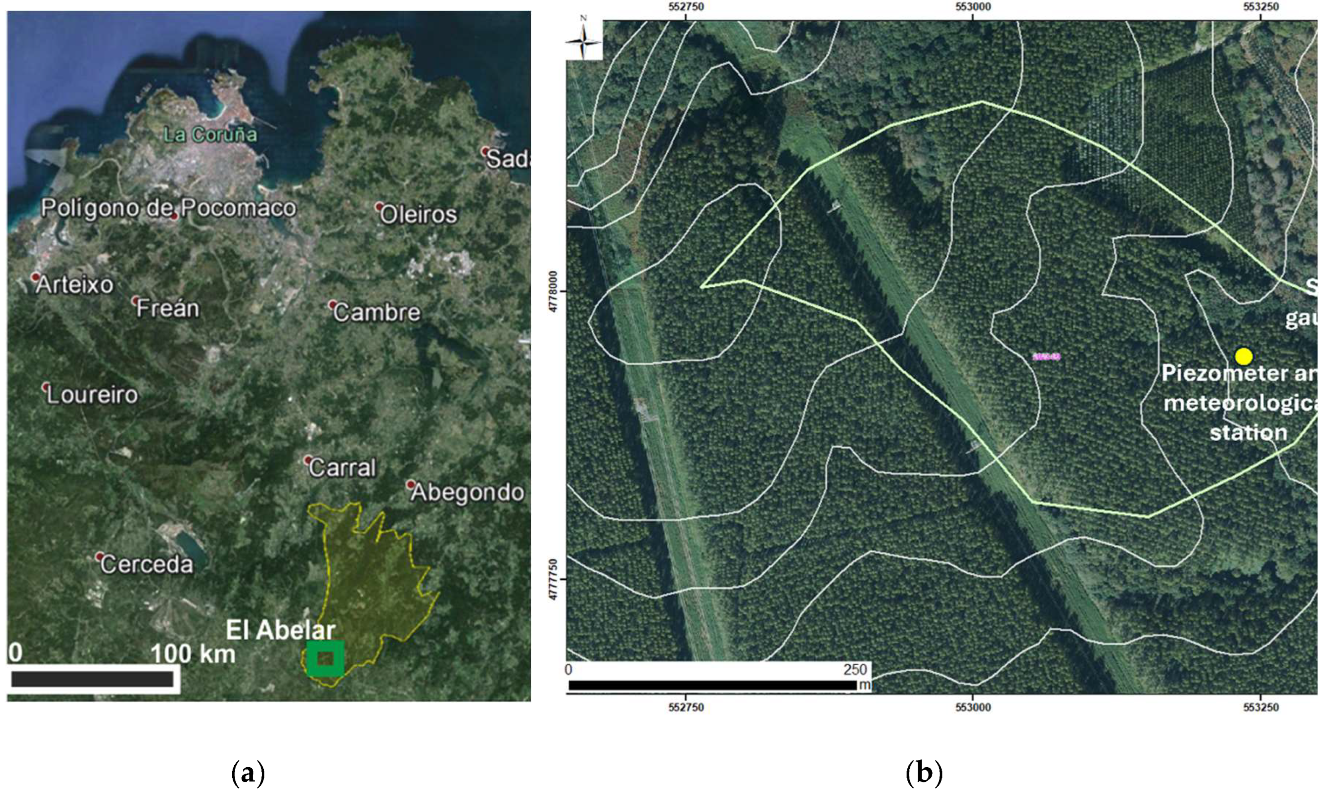
Figure 2.
Stacked area chart displaying daily values of precipitation and streamflow components.
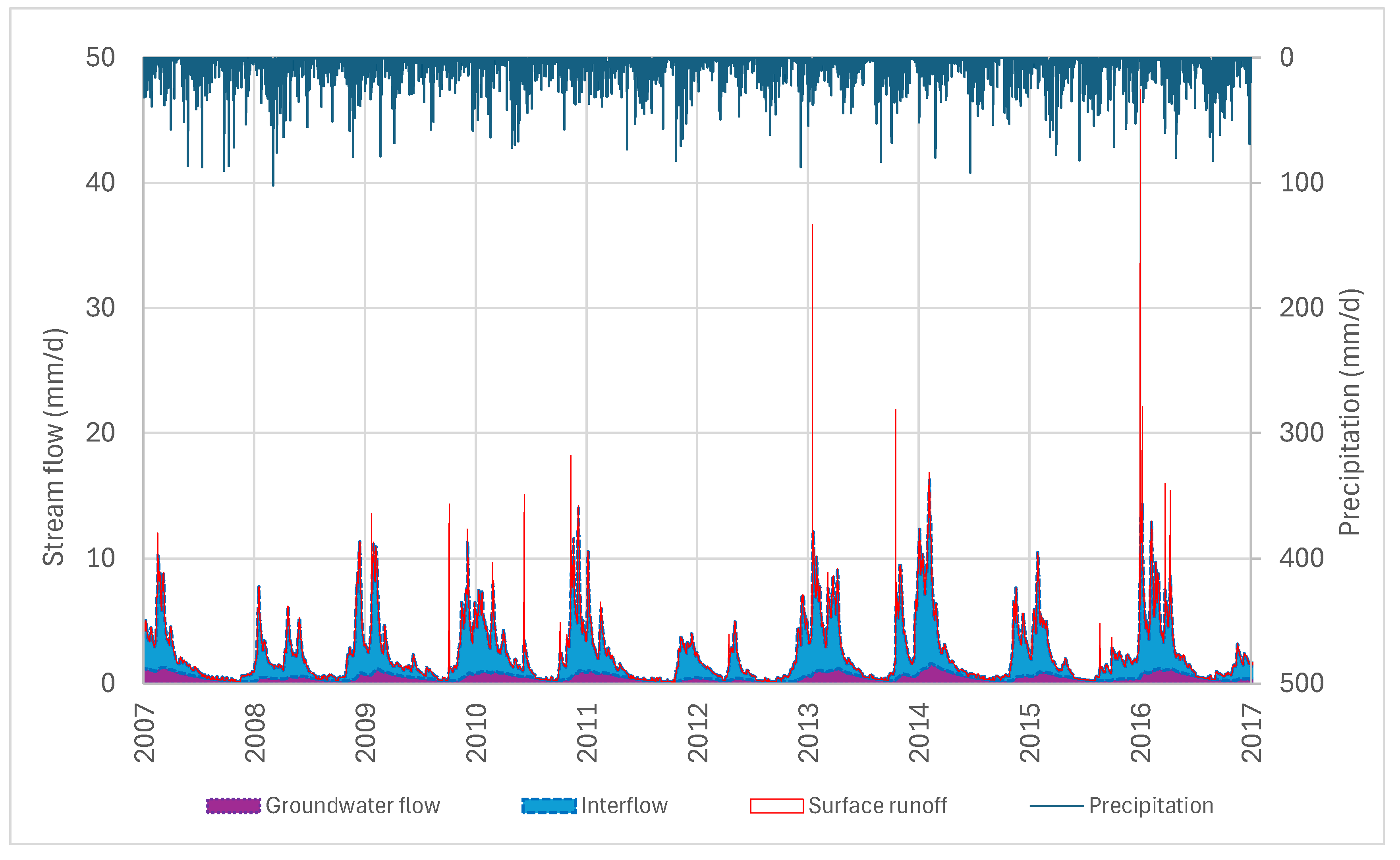
Figure 3.
Time evolution of daily streamflows calculated with the hydrological water balance model (lines) and measured chemical data of chloride and nitrate (a) and Ca, Mg and K data (b).
Figure 3.
Time evolution of daily streamflows calculated with the hydrological water balance model (lines) and measured chemical data of chloride and nitrate (a) and Ca, Mg and K data (b).
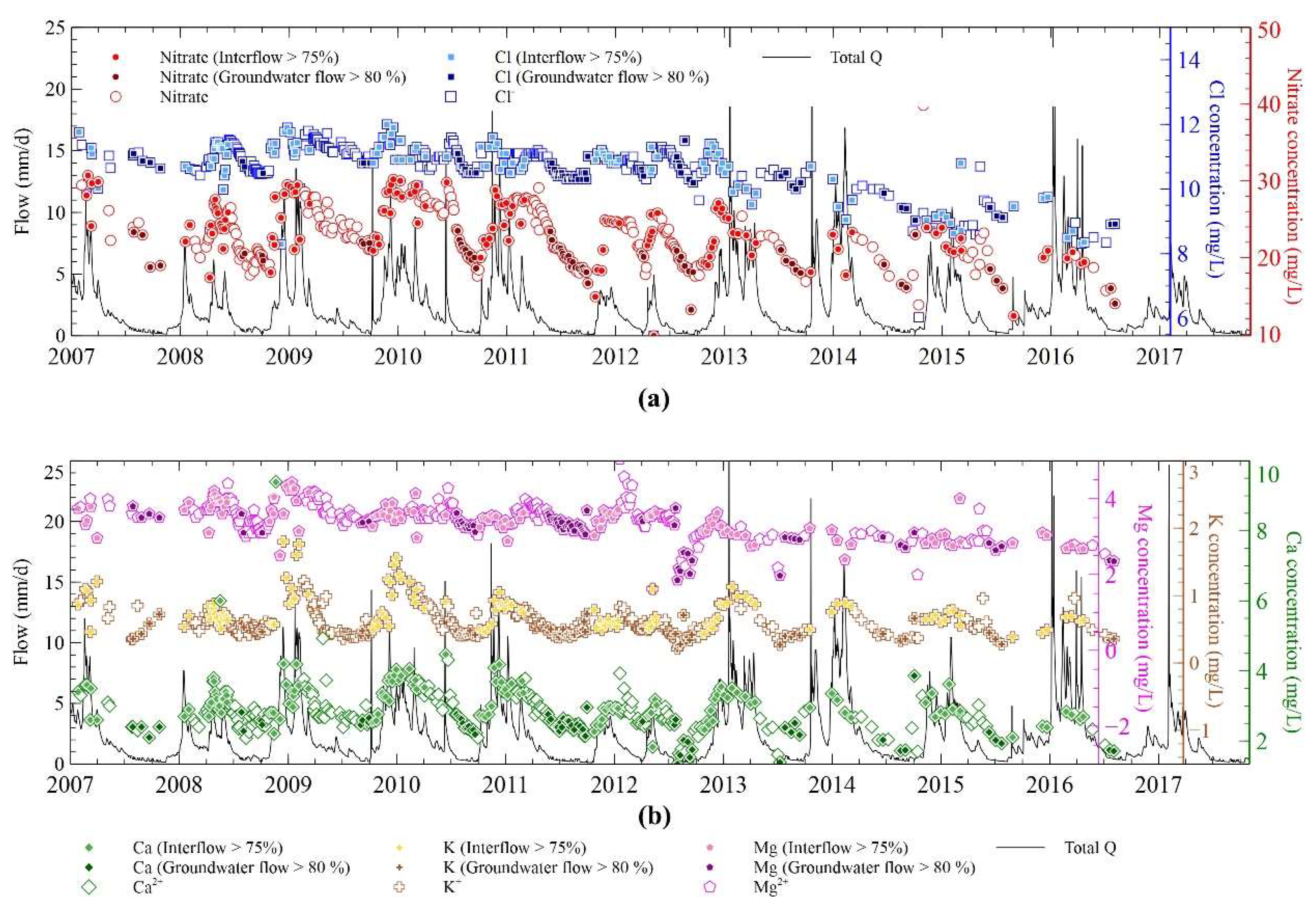
Figure 4.
Flowchart of the methodology of CA modeling in this study.
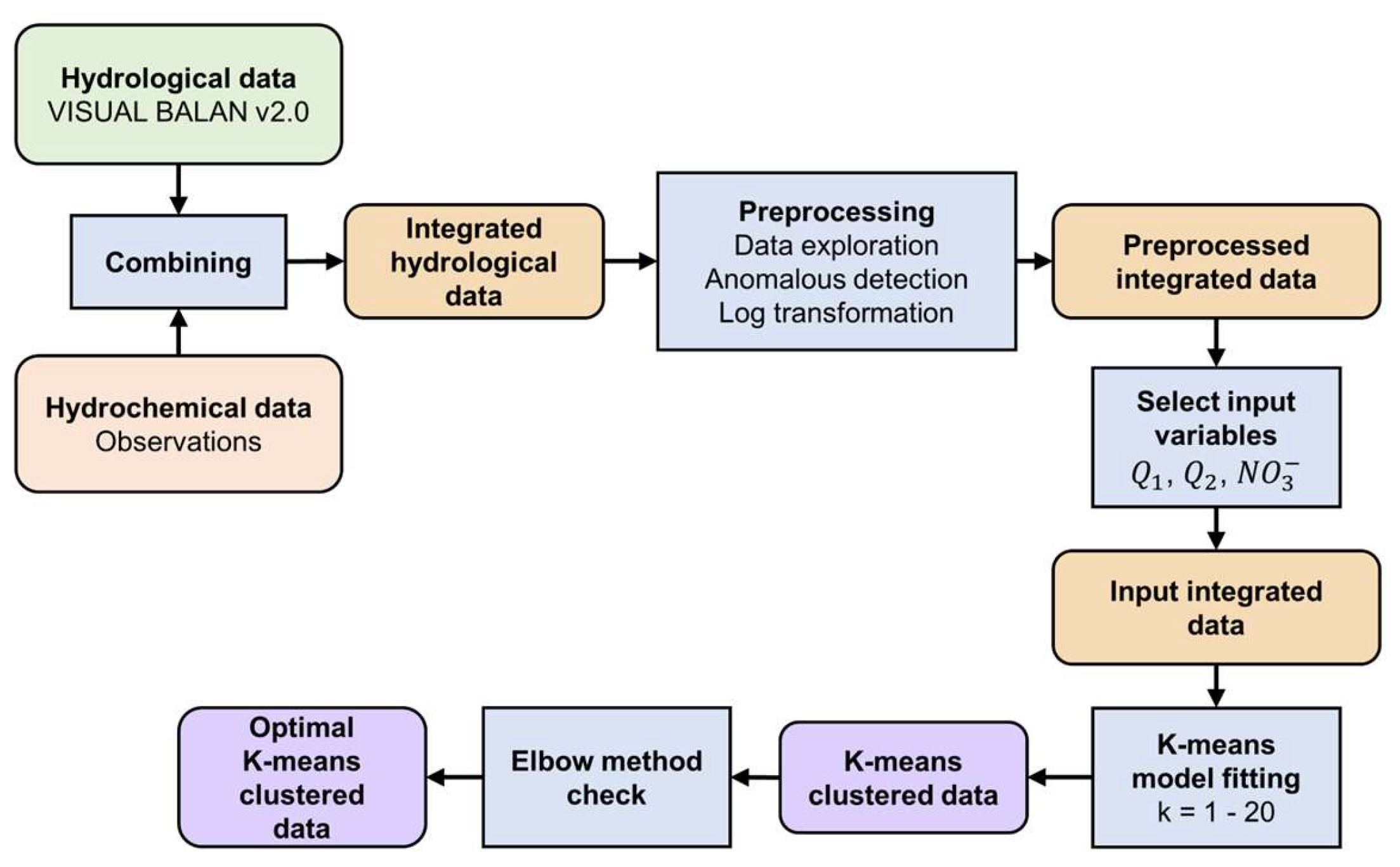
Figure 5.
Flowchart of the methodology for the TS-GPR modeling in this study.
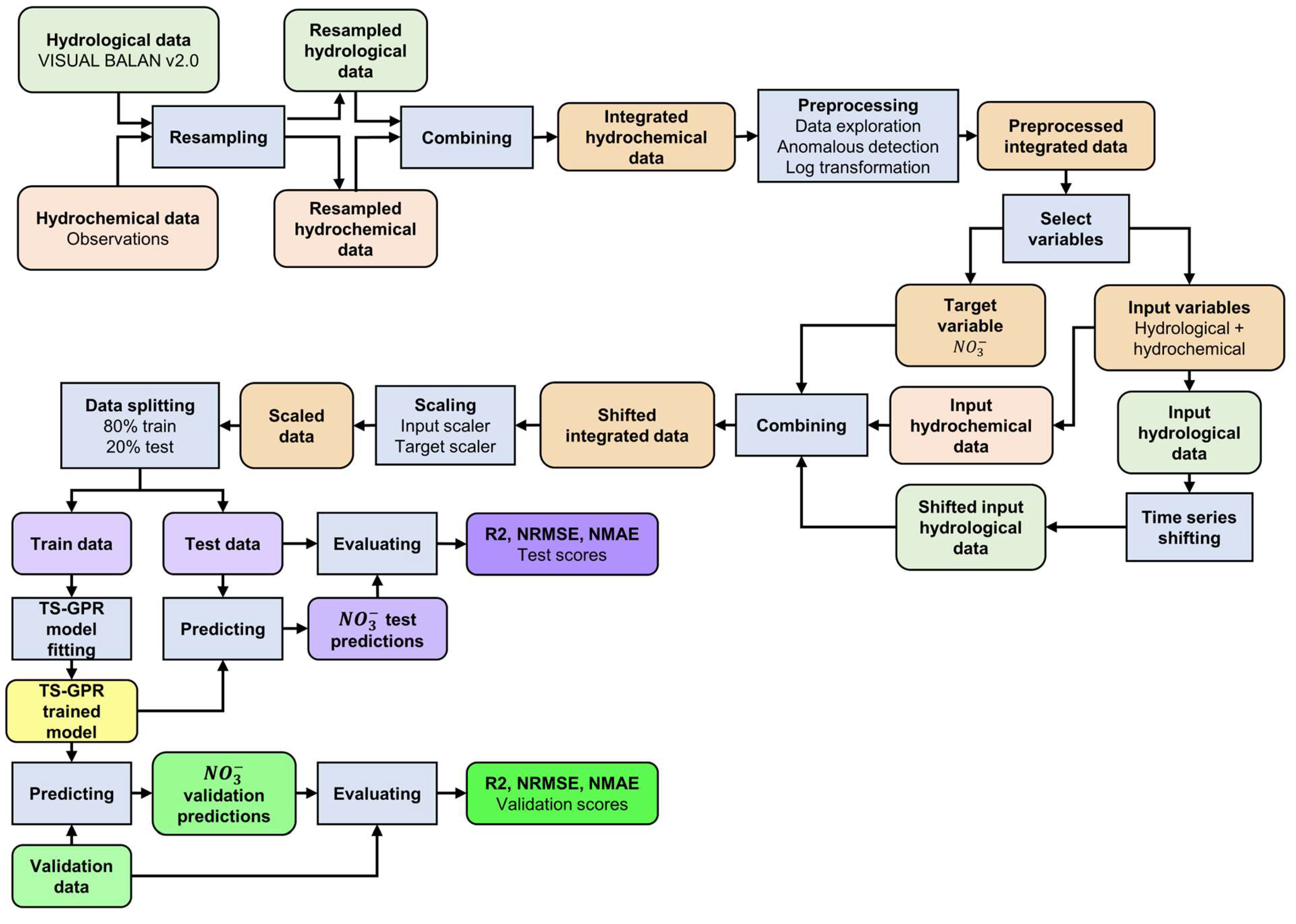
Figure 6.
Plot of inertia versus number of clusters for twenty K-means models fitted on , and nitrate data. The optimal number of clusters (three) corresponds to the elbow of the curve where the slope of the curve visibly bends from high to low slope.
Figure 6.
Plot of inertia versus number of clusters for twenty K-means models fitted on , and nitrate data. The optimal number of clusters (three) corresponds to the elbow of the curve where the slope of the curve visibly bends from high to low slope.
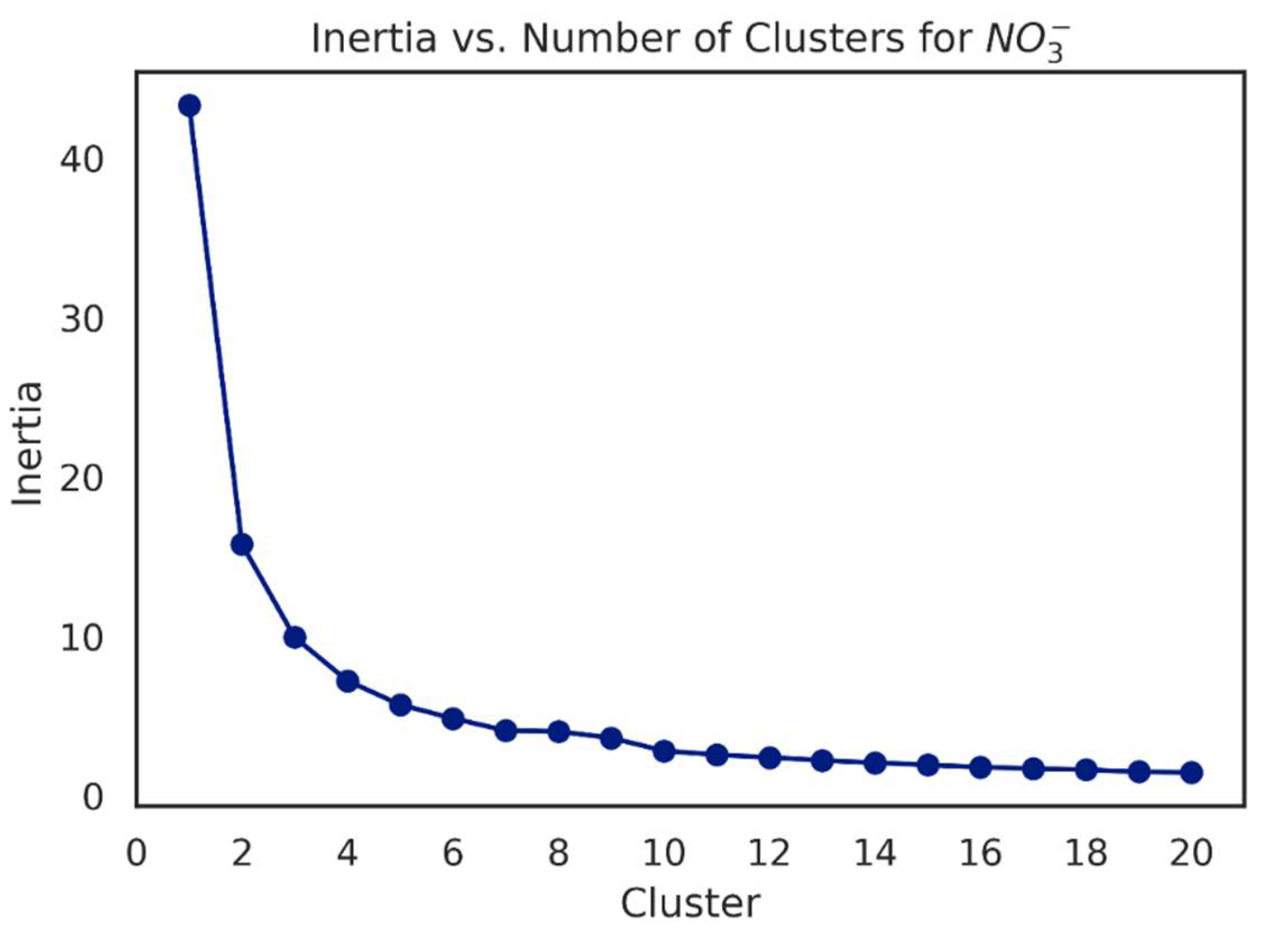
Figure 7.
(a) Pair plot of nitrate concentration (mg/l) versus groundwater flow fraction . (b) Time series plot of nitrate concentration (mg/l) clustered data. The plot shows the three clusters identified by K-means.
Figure 7.
(a) Pair plot of nitrate concentration (mg/l) versus groundwater flow fraction . (b) Time series plot of nitrate concentration (mg/l) clustered data. The plot shows the three clusters identified by K-means.
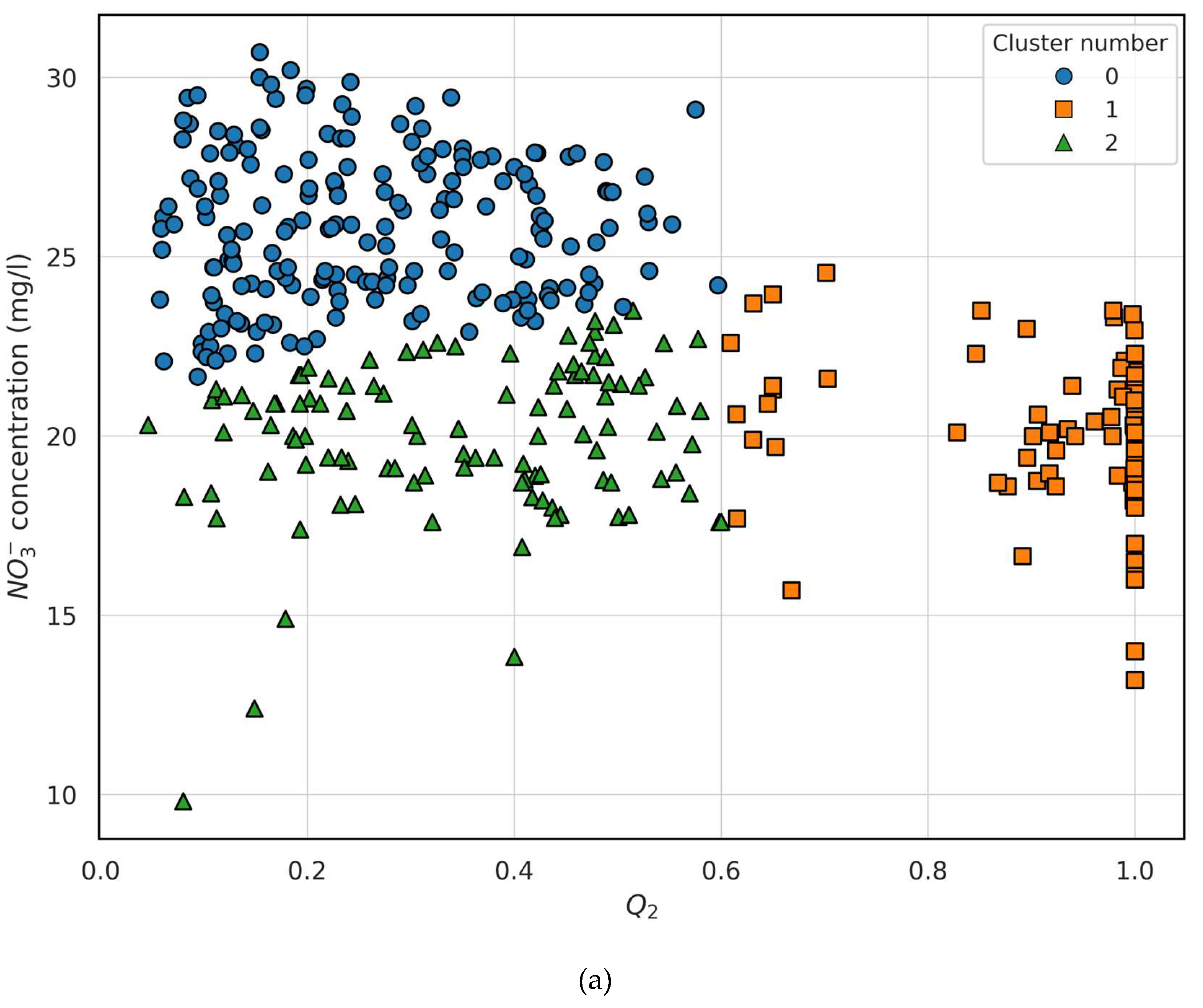
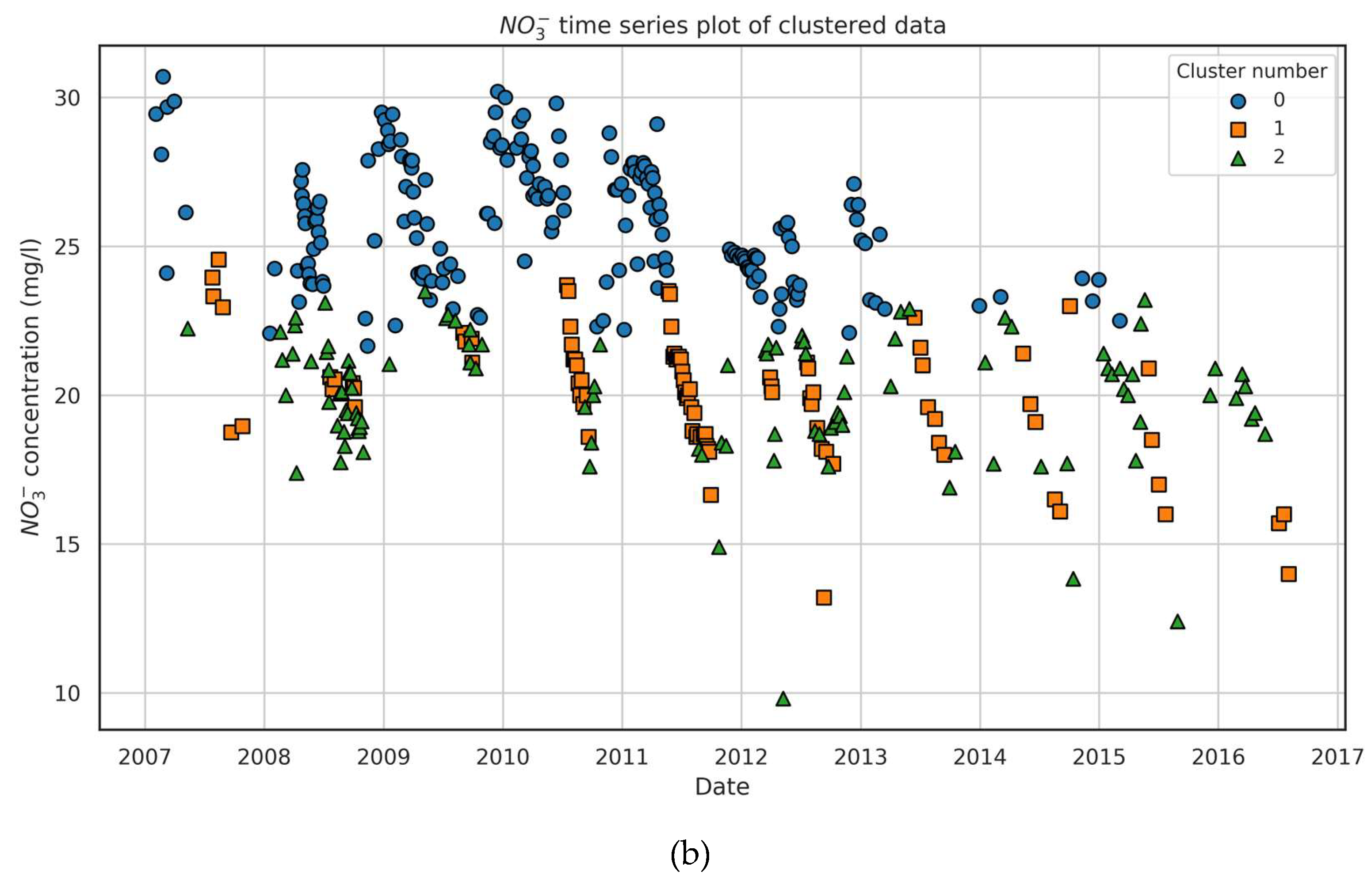
Figure 8.
Scatter plots of predicted versus tested nitrate concentrations on the training (left plots) and testing sets (right plots) for: (a) baseline model, (b) model with best correlated hydrological variables, (c) model with best correlated hydrological variables and shifting (10 days), and (d) model with best correlated hydrological variables, shifting (10 days) and chemical variables. The training results are based on k-fold cross-validation of the training set with 10 folds and 10 repeats.

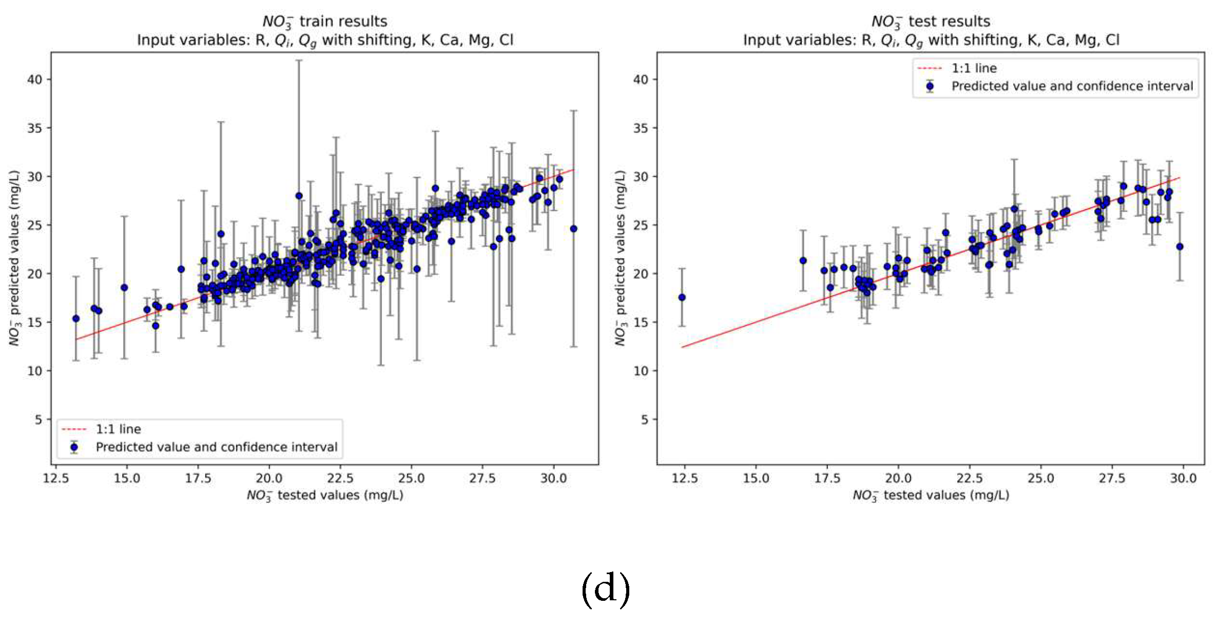
Figure 9.
Time series plot of predicted versus tested nitrate concentrations. The plot illustrates the close alignment between observed and predicted nitrate concentrations over time, along with moderately narrow confidence intervals.
Figure 9.
Time series plot of predicted versus tested nitrate concentrations. The plot illustrates the close alignment between observed and predicted nitrate concentrations over time, along with moderately narrow confidence intervals.
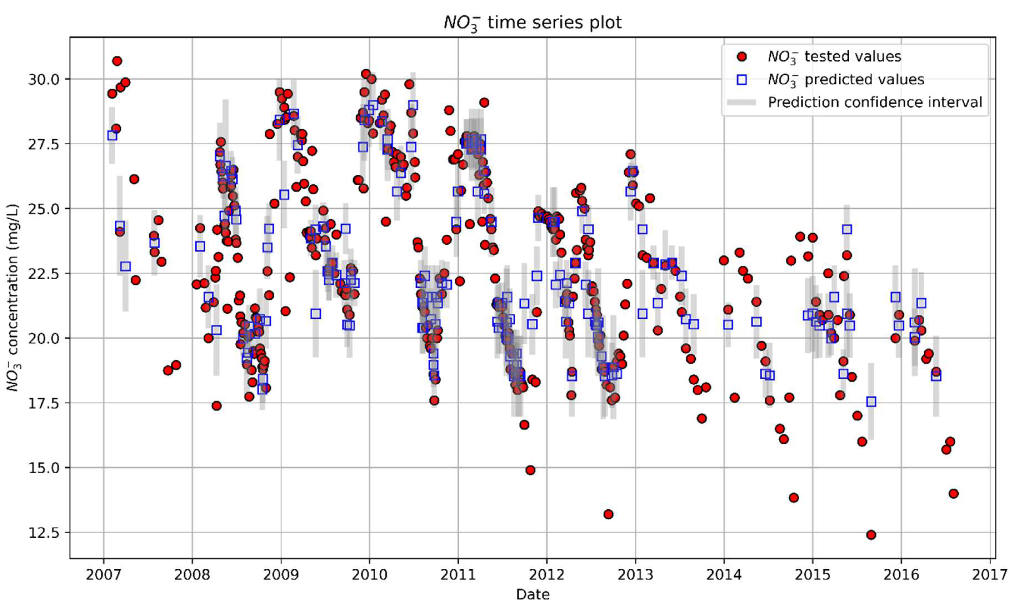
Figure 10.
Boxplot of permutation feature importance on the testing set. The plot shows the relevance of the time series approach with groundwater flow five days before the current date () as the most important variable. The concentrations of Cl, Ca an Mg are also relevant as they cause great decreases in R2 score when shuffled.
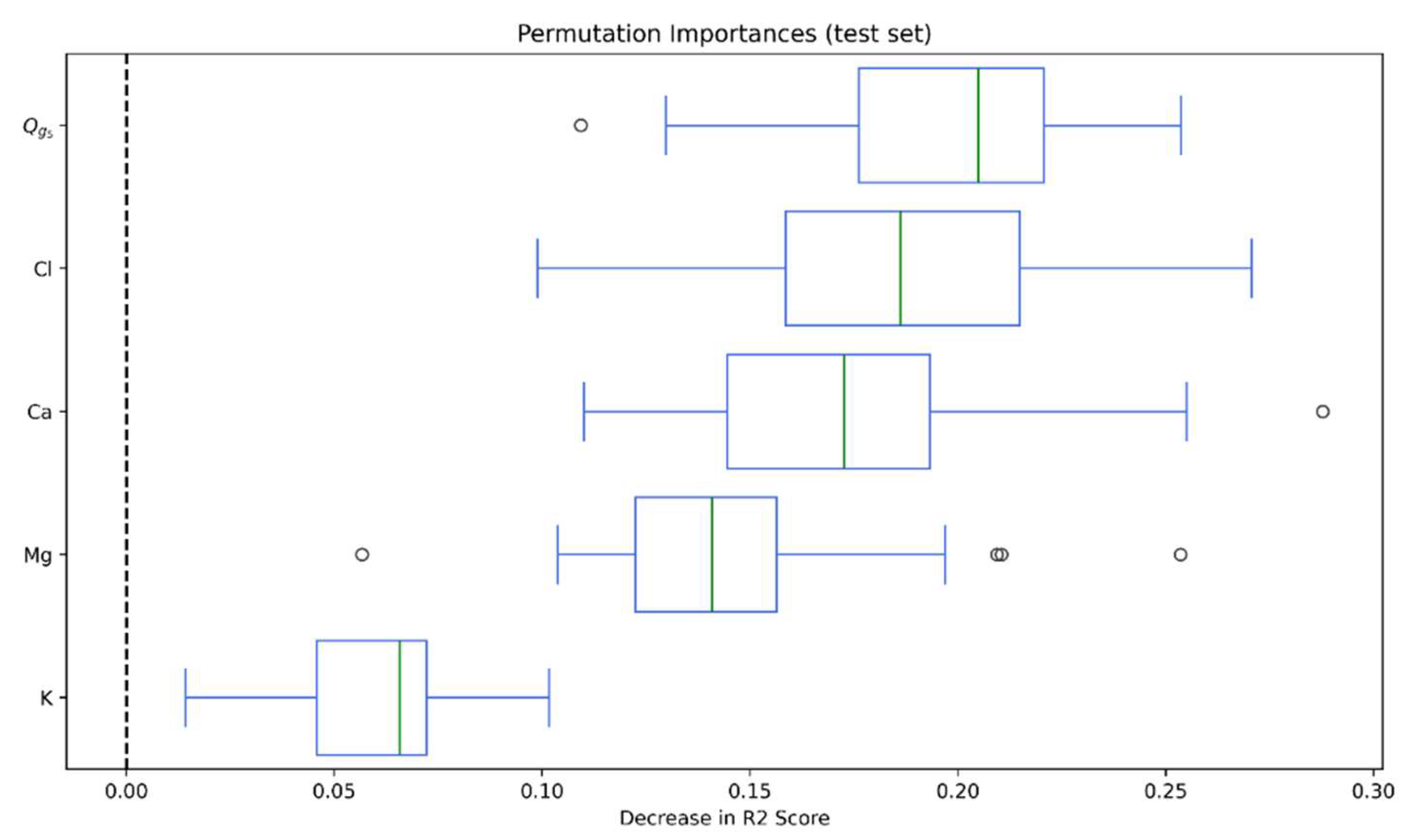
Figure 11.
PDP plots of variables and Cl (a), and Ca and Mg (b). The rightmost plots show an interaction effect between each pair of variables. All variables are unitless after scaling.
Figure 11.
PDP plots of variables and Cl (a), and Ca and Mg (b). The rightmost plots show an interaction effect between each pair of variables. All variables are unitless after scaling.
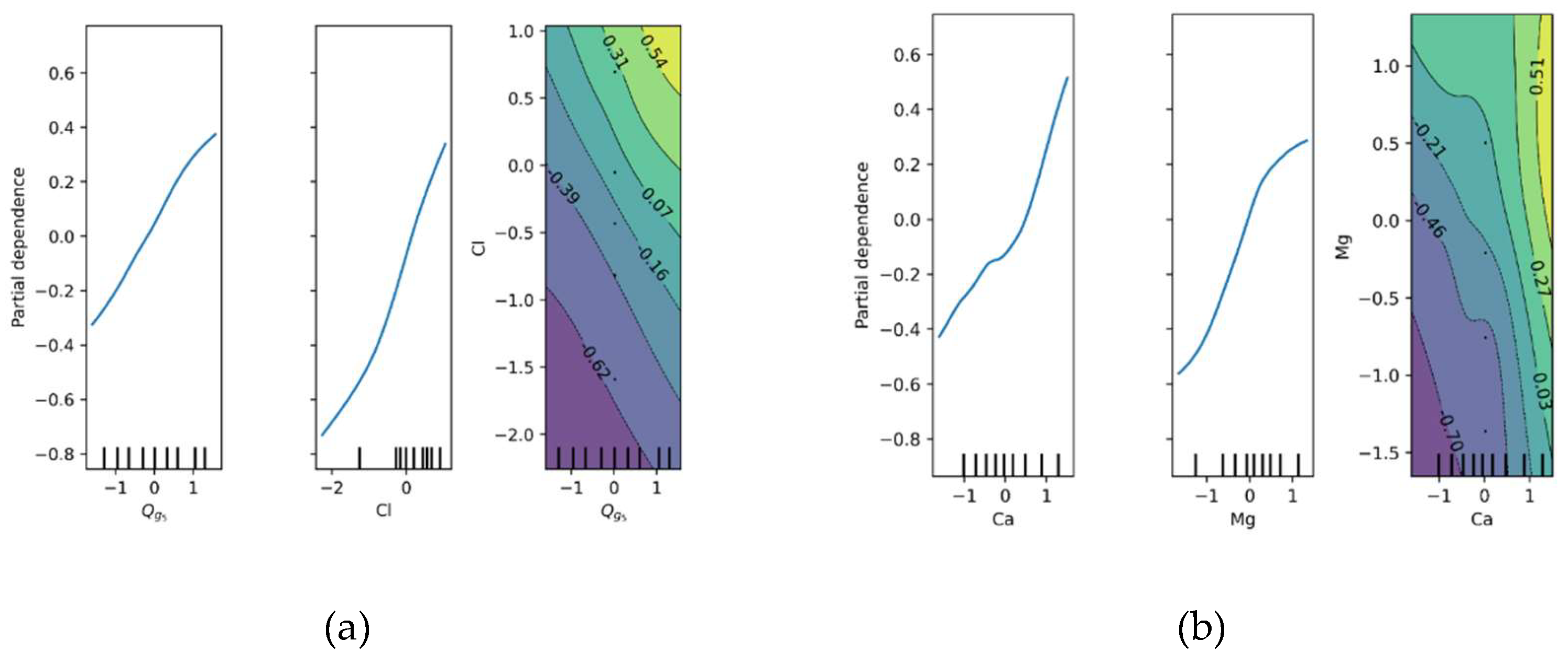
Figure 12.
ICE plots of variables and Cl (a), and Ca and Mg (b). Both pairs of variables have a positive effect on the model’s predictions. The dashed orange lines indicate that on average, increases in each pair of variables lead to higher nitrate concentrations.
Figure 12.
ICE plots of variables and Cl (a), and Ca and Mg (b). Both pairs of variables have a positive effect on the model’s predictions. The dashed orange lines indicate that on average, increases in each pair of variables lead to higher nitrate concentrations.
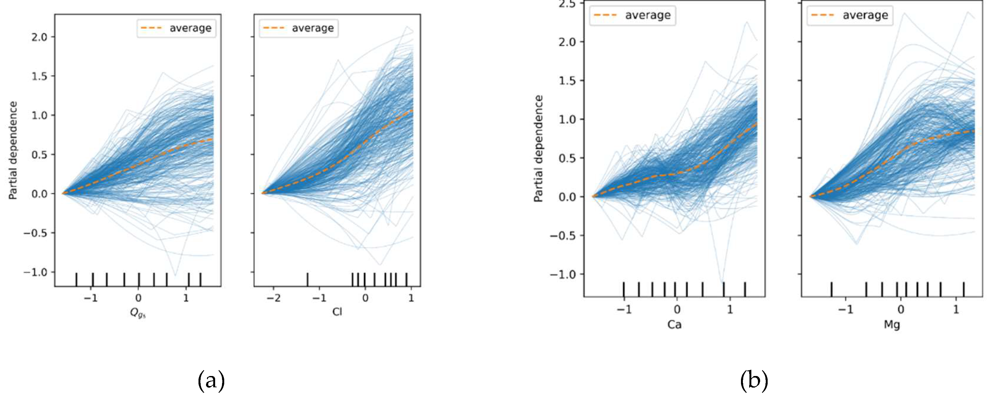
Figure 13.
Scatter plot of predicted versus tested nitrate concentrations for the TS-GPR model of Step 4 (with shifting of the best correlated hydrological variables and chemical variables) on the validation set.
Figure 13.
Scatter plot of predicted versus tested nitrate concentrations for the TS-GPR model of Step 4 (with shifting of the best correlated hydrological variables and chemical variables) on the validation set.
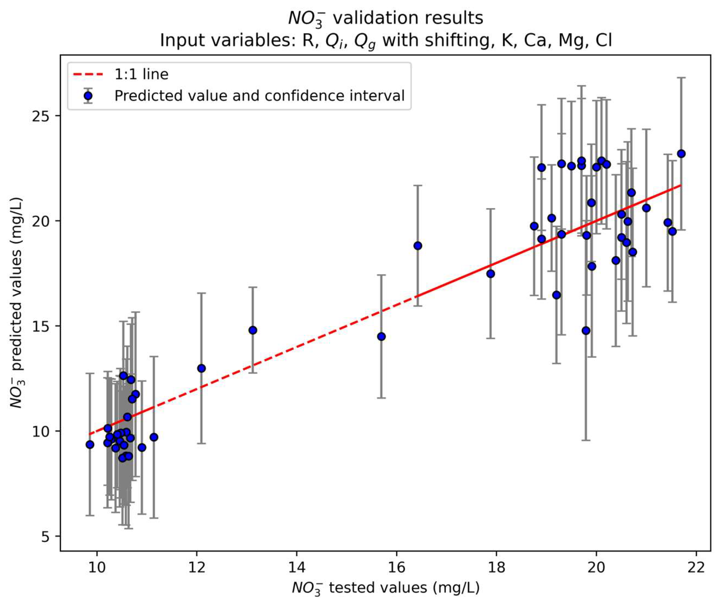
Figure 14.
Time series plot of predicted versus tested nitrate concentrations on the validation set. The plot illustrates the close alignment between observed and predicted nitrate concentrations over time, along with moderately narrow confidence intervals.
Figure 14.
Time series plot of predicted versus tested nitrate concentrations on the validation set. The plot illustrates the close alignment between observed and predicted nitrate concentrations over time, along with moderately narrow confidence intervals.
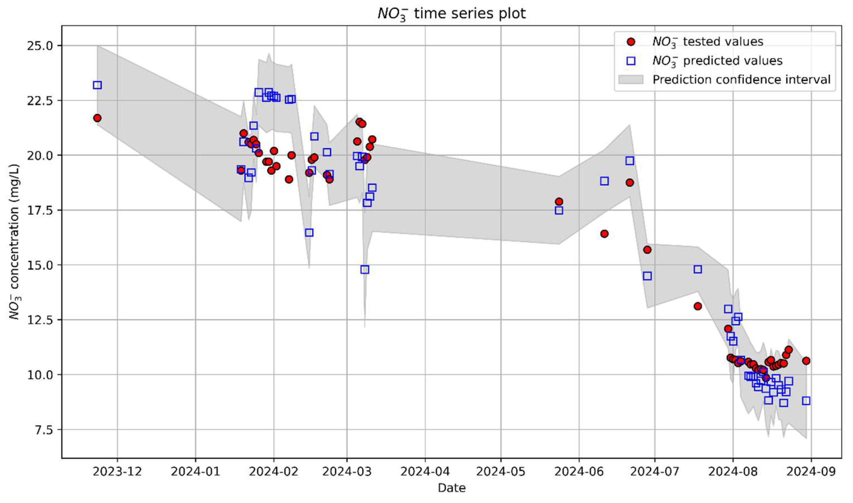

Table 1.
Attributes of the Abelar dataset.
| Name of attribute | Description | Units |
|---|---|---|
| Date | Date of the observation | - |
| P | Precipitation | mm |
| R | Recharge | mm |
| Surface runoff | mm | |
| Interflow/subsurface flow | mm | |
| Groundwater flow | mm | |
| Total flow | mm | |
| K | Potassium concentration | mg/L |
| Na | Sodium concentration | mg/L |
| Ca | Calcium concentration | mg/L |
| Mg | Magnesium concentration | mg/L |
| Fe | Iron concentration | µg/L |
| Mn | Manganese concentration | µg/L |
| Cu | Copper concentration | µg/L |
| Zn | Zinc concentration | µg/L |
| Al | Aluminum concentration | µg/L |
| Vn | Vanadium concentration | µg/L |
| Si | Silicon concentration | mg/L |
| Cl | Chloride concentration | mg/L |
| Sulfate concentration | mg/L | |
| Nitrate concentration | mg/L |
Table 2.
Descriptive statistics of the CA clusters across nitrate data.
| Cluster number | |||
|---|---|---|---|
| Statistic | 0 | 1 | 2 |
| count | 179 | 76 | 133 |
| mean | 25.156 | 19.802 | 21.333 |
| std | 2.860 | 2.037 | 3.296 |
| min | 17.700 | 13.200 | 9.809 |
| 25% quantile | 23.114 | 18.674 | 19.099 |
| 50% quantile | 25.399 | 20.049 | 21.400 |
| 75% quantile | 27.500 | 21.124 | 23.779 |
| max | 30.699 | 23.499 | 29.099 |
Table 3.
Descriptive statistics of the CA clusters across (ratio of interflow to total flow) data.
| Cluster number | |||
|---|---|---|---|
| Statistic | 0 | 1 | 2 |
| count | 179 | 76 | 133 |
| mean | 0.793 | 0.026 | 0.548 |
| std | 0.093 | 0.045 | 0.116 |
| min | 0.538 | 0 | 0.297 |
| 25% quantile | 0.730 | 0 | 0.479 |
| 50% quantile | 0.804 | 0 | 0.545 |
| 75% quantile | 0.871 | 0.026 | 0.599 |
| max | 0.942 | 0.171 | 0.919 |
Table 4.
Descriptive statistics of the CA clusters across (ratio of groundwater flow to total flow) data.
Table 4.
Descriptive statistics of the CA clusters across (ratio of groundwater flow to total flow) data.
| Cluster number | |||
|---|---|---|---|
| Statistic | 0 | 1 | 2 |
| count | 179 | 76 | 133 |
| mean | 0.205 | 0.973 | 0.447 |
| std | 0.093 | 0.045 | 0.120 |
| min | 0.057 | 0.828 | 0.046 |
| 25% quantile | 0.127 | 0.973 | 0.398 |
| 50% quantile | 0.195 | 1 | 0.452 |
| 75% quantile | 0.269 | 1 | 0.515 |
| max | 0.460 | 1 | 0.703 |
Table 5.
Training, testing and validation metrics of accuracy of TS-GPR models across the different steps of the modeling process. Metrics include R2, NRMSE and NMAE. Training metrics correspond to repeated k-fold cross-validation on the training set (10 folds, 10 repeats).
Table 5.
Training, testing and validation metrics of accuracy of TS-GPR models across the different steps of the modeling process. Metrics include R2, NRMSE and NMAE. Training metrics correspond to repeated k-fold cross-validation on the training set (10 folds, 10 repeats).
| Metrics of accuracy | |||||
|---|---|---|---|---|---|
| Step | Input variables | Case | R2 | NRMSE | NMAE |
| 1 | Training | 0.07 | 0.19 | 0.15 | |
| Testing | 0.13 | 0.20 | 0.15 | ||
| 2 | R, , | Training | -0.01 | 0.19 | 0.15 |
| Testing | 0.22 | 0.19 | 0.15 | ||
| 3 | R, , with shifting | Training | 0.44 | 0.14 | 0.10 |
| Testing | 0.45 | 0.16 | 0.11 | ||
| 4 | R, , withshifting and K, Ca, Mg, Cl | Training | 0.82 | 0.08 | 0.05 |
| Testing | 0.80 | 0.10 | 0.06 | ||
| Validation | R, , withshifting and K, Ca, Mg, Cl | Validation | 0.85 | 0.15 | 0.12 |
Disclaimer/Publisher’s Note: The statements, opinions and data contained in all publications are solely those of the individual author(s) and contributor(s) and not of MDPI and/or the editor(s). MDPI and/or the editor(s) disclaim responsibility for any injury to people or property resulting from any ideas, methods, instructions or products referred to in the content. |
© 2025 by the authors. Licensee MDPI, Basel, Switzerland. This article is an open access article distributed under the terms and conditions of the Creative Commons Attribution (CC BY) license (http://creativecommons.org/licenses/by/4.0/).
Copyright: This open access article is published under a Creative Commons CC BY 4.0 license, which permit the free download, distribution, and reuse, provided that the author and preprint are cited in any reuse.


