Submitted:
02 March 2025
Posted:
03 March 2025
You are already at the latest version
Abstract
A method is introduced for the numerical continuation of the lunar-type, near-circular periodic orbits, with the background of middle-altitude lunar orbiters. In the Moon-Earth elliptic restricted three-body problem, some near-polar near-circular lunar-type periodic orbits are numerically continued from the Keper circular orbits by Broyden’s method. The integer ratio j/k of the mean motions between the inner and outer orbits can be in the range [9,150]. For the ratio j/k∈[38,70], the J2,C22 perturbations are added, and some near-polar periodic orbits are calculated. The orbital dynamics are well explained via the first-order double-averaged system. The linear stability can be studied by the characteristic multipliers, which are calculated from the linear variational system.
Keywords:
Periodic orbits
; Restricted three-body problem
; Lidov–Kozai effect
; linear stability
; Lunar orbiter
1. Introduction
Nowadays, with the increasing demand for the lunar exploration and the development of the aerospace technology, the cislunar space is becoming a new frontier for human activities. In order to carry out long-term scientific research missions near the Moon and save fuel for placing a space station, it is necessary to use the stable and approximately stable orbits, such as distant retrograde orbits (DROs), near-rectlinear halo orbits (NRHOs) and near-polar frozen orbits [1]. It is a common idea to firstly study the periodic orbits of the restricted three-body problem (RTBP), then continue the solutions to a generalized time-periodic model, and lastly to a high-fidelity ephemeris model[2]. It is important to study periodic orbits as they help us to understand the real motions, and there is a long history on this study. Ever since the excellent work of H. Poincaré, periodic orbits have aroused the attentions of many mathematicians, astronomers, celestial mechanicians, and so on[3,4].
The family of the near-polar and near-circular periodic orbits are interesting. According to Poincaré’s classification, these periodic orbits belong to the third-type of the first kind. The existence of this family in the elliptic RTBP is shown by Xu and Fu [5]. Theoretically, these periodic orbits are very close to one primary. Numerically , Xu and Song [6] found that these orbits can be of high altitude, and some other interesting phenomena were found as well. The eccentricity and the inclination of such a periodic orbit vary periodically and satisfy the Lidov-Kozai effect. For some values of the eccentricity of the outer orbit and the ratios of the mean motion resonances between the inner and outer orbits, the periodic orbits can be approximately linearly stable. This assures the the judgement that the high-altitude and near-circular polar frozen orbits are suitable to place a lunar station[7]. However, Xu and Song [6] did not give enough details about the near-polar and near-circular lunar-type periodic orbits. For a further study, it makes sense to study the these long-period periodic orbits in a more accurate gravity field model.
The motion of a lunar orbiter with the altitude in the range km is mainly affected by the gravitation of the Moon-Earth system. The Moon-Earth system can be simplified as a two-body system, while the Moon can be considered as a triaxial ellipsoid, as the main non-spherical perturbations come from the terms. The zonal coefficient represents the size of the oblateness, and the sectorial coefficient measures the equatorial ellipticity. The obliquity of the Ecliptic plane and Moon’s Path is neglected. There is an interesting phenomenon named tidal locking for the Moon, that is, the rotation period and the revolution period are nearly equal, and the longest axis always passes the Earth. For lower-altitude lunar orbits, Lara et al. [8] studied the long-term dynamics of the near-polar frozen orbits by reducing a 50-degree zonal model with the third-body effect of the Earth. Saedeleer [9] explained the Hamiltonian system of a lunar orbiter in the Moon-Earth circular RTBP with perturbations, and studied the averaged system by the Lie-Deprit method. With the same model, Nie and Gurfil [10] studied the lunar frozen orbits in the first-order double-averaged system in Delaunay elements by Zeipel’s method. For the frozen orbits, the slow mean orbital elements keep nearly fixed such that the costs of the orbital corrections are reduced.
With the perturbations and several orders of the Legendre expansions of the third-body perturbations, Carvalho et al. [11] studied frozen orbits and the critical inclinations of the lunar satellites by analyzing the double-averaged system. Considering the 3rd-degree gravity harmonics of the Moon, Tzirti et al. [12] investigated the Poincaré sections, the Fast Lyapunov Indicator Maps and some families of periodic orbits. Tzirti et al. [13] studied the secular dynamics of low-altitude lunar orbiters with high-degree gravity models by the frequency analysis and investigated the eccentricity-inclination space. Considering a lunar orbiter perturbed by the terms, El-Salam and El-Bar [14] investigated the families of frozen orbits. In Sirwah et al. [15], the perturbing function is considered up to the seventh zonal harmonic and the third-body perturbation of the Earth in an elliptic inclined orbit. Then they numerically studied the frozen orbits with the arguments of the pericenter at . An efficient approach based on the grid search, parallelization and the evolution strategy is introduced for computing periodic orbits in Dena et al [17]. Franz and Russell [18] introduced the database of the symmetric periodic orbits near Moon in the model of the circular RTBP via the grid search and unsupervised learning clustering algorithm. Legnaro and Efthymiopoulos [19] distinguished three types of lunar orbits by the range of altitudes, and studied the secular dynamics especially the secular resonances and the eccentricity growth of lunar satellites according to different models.
In Section 2, we provide a new approach to do the numerical continuation of the near-polar and near-circular periodic orbits of the elliptic RTBP, and give some numerical examples of the lunar-type periodic orbits. In Section 3, we study the existence and stability of the near-polar and near-circular periodic orbits in the elliptic RTBP with the perturbations. Some numerical examples are also given. Finally, Section 5 concludes this work.
2. Elliptic RTBP
2.1. Scaled Hamiltonian System
With the background of the motion of a lunar orbiter in the cislunar space, we study the periodic orbits around the smaller primary in the elliptic RTBP. Let and represent two mass points. The relative orbit from to is a Keplerian orbit, with the semi-major axis , the eccentricity , the mean motion , and the time of periapsis passage . Choose the units such that the gravitational constant , the distance unit , the total masses , and the mean motion . Let . Set the motion plane of primaries as the reference plane. The direction of the major axis from to is set as the -axis. Set as the origion and establish the right-handed Cartesian coordinate system . The initial time is set as or . The sketch figure of the frame can be referred to [5].
In the coordinate system , the position of is denoted as , which is also a solution of the planar Kepler problem
Here represent the Euclidean distance norm, and the time is t. We have . Denote as the eccentric anomaly. The vector is
where the upper represents transpose. The position of the infinitesimal body is , and its conjugate momentum is . The Hamiltonian dynamical system of this problem is
The canonical differential equation system is , . The 2nd-order differential equation system can be written as
When is very small, it is not convenient to get the numerical solution, as the orbit scale is too small.
The orbit of the infinitesimal body is called as the inner orbit, and the orbit of the relative orbit of is the outer orbit. Denote the orbital elements of the inner orbit as , , , , , , where ℓ represents the mean anomaly. According to the symplectic scaling method, the variables can be scaled as
where s is the new time, and the small parameter represents the closeness of the infinitesimal body to primary . The new Hamiltonian is
The new differential equation system becomes
where , , and the prime represents the derivative about the scaled time s. Let be the scaled variable and . We have , and , so . It is convenient to set if . Then we get . The Kepler equation for the outer orbit satisfies
The numerical solution of Eq. (5) can be calculated by the integration effectively.
2.2. Symmetry and Periodicity
The scaled Hamiltonian system keeps the same symmetries as the original Hamiltonian system . One time reversing symmetry with respect to -axis is recalled.
There exist periodic third-body perturbations in the lunar-type orbits in the elliptic RTBP. The desired periodic orbits can be continued from the two uncoupled Kepler orbits. The ratio of the mean motions of the uncoupled inner and outer Kepler orbits is set to be , and should be a small rational number. is set to equal , where and . This means that the inner orbit revolves j circles while the outer orbit revolves k circles. In order to understand the -symmetric periodic solution, a proposition is summarized as follows.
Lemma 1
([5]). For the Hamiltonian system (1) of the elliptic RTBP. The Lagrangian set with respect to -symmetry is
If a solution satisfies and with , then the solution is -symmetric and periodic with a period . For the Hamiltonian system (4), the corresponding Lagrangian set is
and the scaled periodic solution has a period with . The ratio of the mean motions of the outer and inner orbits is . The periodicity conditions used in this paper can be written as
According to the description in Xu and Song [6], there exist both near-polar and planar -symmetric near-circular lunar-type periodic orbits in the elliptic RTBP. However, Xu and Song [6] did not give enough details of the numerical continuation of such periodic orbits. The difficulty lies at the fact that the accumulated integration errors are relatively large when the infinitesimal body is very close to primary and the integration time is long. For the Hamiltonian system (1), the initial values to be continued can be written as
The scale of the lunar-type orbits are small but the velocities are relatively big. For the Hamiltonian system (4), the initial values to be continued can be written as
In this paper, the scaled variables are used and more numerical continuation results can be achieved. The continuation scenario is still based on the combination of the periodicity conditions and Broyden’s method with a line search. This means that is expected to be continued to
such that
where are small quantities, and .
2.3. Some Periodic Orbits
The numerical solutions of Eq.(5) are calculated by the variable step-size Runge-Kutta 7-8 routine with the double precision. The routines of Broyden’s method are referred to Press et al. [16] and the precision is guaranteed at . So the periodic orbits can keep the precision of . Let represent the Earth and the Moon, respectively. Let , . Set as the ratio of the mean motions between the uncoupled inner and outer orbits. The real length of the semi-major axis of the outer orbit is about km. The real length of the semi-major axis of the inner orbit is about km with . The altitude is defined as the difference of and the real length of the longer equatorial semi-major axis km. The high altitude zone is defined in the range about between 5000km and 20000km. In this zone, the third-body perturbation of the Earth is dominant. In the theoretical proof of the existence of the near-polar and near-circular periodic orbits in the elliptic RTBP, the small parameter is supposed to be small enough. One question is that how small is is when the periodic orbits can be calculated. Such periodic orbits are numerically investigated with in the range . In Figure 1 and Figure 2, it is found that the argument of pericenter rotates and oscillates. Figure 3 is for the case . All these orbital elements are very symmetric. The details of the figures are shown in the image captions. Some more initial values for the periodic orbits are shown in Table 1. The type of the initial values are defined by the signs of the values of and .
3. Elliptic RTBP with Perturbations
3.1. The Model and Numerical Experiment
The usual orbital elements are the semi-major axis a, the eccentricity e, the inclination i, the longitude of the ascending node , the argument of the periapsis , and the mean anomaly M. The eccentric anomaly is notated as , and the true anomaly is notated as . If just the perturbations of are added to the RTBP, the application of this model is for the case of the altitude about in the range km. The non-spherical perturbing function is usually expressed by orbital elements. It is necessary to transform the perturbing function into the form of Cartesian coordinates for the convenience of the computation of the near-circular periodic orbits. For a massless artificial satellite in the Moon-centered inertial coordinate frame, the position is notated as , and the conjugate momentum is . The Hamiltonian system of a lunar orbiter can be written in a form of perturbations of the RTBP,
where
and
In order to better understand the angles and , Figure 4 is recomanded for reading. In the Lunar inertial coordinate frame , the longitude of the ascending node of the infinitesimal satellite is , and the latitude is . The prime meridian is set at the direction of the longest semi-major axis of the ellipsoid. The longitude of the satellite is in the rotating frame . The Earth is always on the -axis. Besides, is notated as the true anomaly of the outer orbit, is the 2nd-order Legendre polynomial, and is the unnormalized associative Legendre polynomial.
With the help of the symplectic scaling,
and the Legendre polynomial expansion[5], the Hamiltonian (7) becomes
where
The relations between the scaled rectangular coordinates and the osculating orbital elements are
Here, , and can be expressed as
where
According to the knowledge of the complex variable functions, the real triangular functions can be replaced by the complex exponential functions, such that the powers of the real triangular functions are easy to be calculated. By this method, we get
Now, it is convenient to apply the Hamiltonian system (8) both for the numerical computation of the periodic orbits and for the analysis of the first-order perturbed system. By numerical experiment, It is found that is near 0 when and is near when . An example is given in Figure 5. Some more initial values of these frozen periodic orbits can be found in Table 2. It is interesting to explain the phenomenon in the first-order double-averaged system.
3.2. First-Order Averaged System
The scaled canonical Delaunay elements are introduced in order to do the Von Zeipel transform and get the first-order averaged system.
The completely expansion of the perturbed system in the Delaunay elements is difficult, so the mean anomaly ℓ is usually contained in and . Hansen coefficients are usually taken in use in the elliptic expansion[3],
We remove the hats above the Hamiltonian notations in (8). Let . After elimination of the fast variable M, we get
Consider that the second fast variable is , these terms above can be averaged again as
The canonical differential equations of the first-order averaged system are
For a further step, we have
In the near-polar and near-circular frozen orbits, the orbital elements a, e, i, are almost constants with small periodic amplitudes. Substitute the initial unperturbed orbital elements into the differential equation about , we have
If g is fixed at 0 or , we have , but it can just happen for the low-altitude lunar orbits.
In order to understand the periodic behaviors of these frozen orbits, we resort to Poincaré-Delaunay elements, as they are effective for near-circular and near-polar orbits.
The first-order double averaged system in the Poincaré-Delaunay elements can be written as
where
The canonical differential equations can be calculated with the help of a symbolic computation software like the wxMaxima.
The key parts of the differential equations of the first-order double averaged Hamiltonian system (10) are as follows.
In the first-order double-averaged system, and are constants. Set and , we have . The differential equations about can be simplified as
Suppose , then . We have . So there exist polar-type and circular periodic orbits in the first-order double-averaged system.
4. Linear Stability
The Hamiltonian system is
where
The 2nd-order differential equations are
where , and
The canonical differential equations of the Hamiltonian system are
The solution is notated as , . The fundamental solution matrix of the linear variational equations is notated as
The system of the linear variational equations is
where is a identical matrix, is a zero matrix, and
The initial values for Eq. (12) is the identical matrix. The Equations (11) and (12) should be integrated together. The scaled time for the numerical integration is the period of a periodic orbit. However, the whole information of a symmetric periodic orbit can be gotten by the integration of a half period.
the monodromy matrix can by calculated by the following formula[6]
There are three pairs of conjugate eigenvalues for the matrix . If one periodic orbit is linearly stable, the eigenvalues are in the unit circle. If not, at least one eigenvalue will be far away from the unit circle. One index to describe the stability is the summation of the moduli of the eigenvalues. The eigenvalues of are also called characteristic multipliers. For just a few examples, the summation of the moduli of the multipliers can be calculated directly from the eigenvalues of . With the and the third-body perturbations, the stability index for the periodic orbit of -type is about 24, and 114 for the case , 590 for the case case, and 3778 for the case . In the elliptic RTBP, the linear stability index is about 7 for the case . This reveals that it saves fuel at the high-altitude orbits.
5. Discussion
The paper provides a lot information about the near-polar, near-circular, lunar-type periodic orbits in the Moon-Earth elliptic restricted three-body problem with and third-body perturbations. Some periodic orbits are calculated and the orbital dynamics are well explained by the first-order double-averaged system. The symplectic scaling technique is introduced, and the small parameter represents the small ratio of the mean resonances between the inner orbit of the infinitesimal body and the outer orbit of the relative motion of the Earth. The linear stability index is introduced and the linear variational equations are calculated. The scaled Hamiltonian system can also be applied to the study of the near-planar lunar orbits.
More work can be done based on this paper. For high-altitude orbits, the perurbation from the Sun can be added to the Hamiltonian system, and the perturbations can be neglected. The quasi-bicircular model of the Moon-Earth-Sun system can be applied. The asymmetric periodic orbits can be studied with the aim of finding stable orbits. It is interesting to study the analytical solutions and the evolution of the orbits. The formulas of this paper can also be adjusted to study the orbits around a satellite of one planet.
Author Contributions
Conceptualization, X. Xu; methodology, X. Xu; software, X. Xu; validation, X. Xu; formal analysis, X. Xu; investigation, X. Xu; resources, X. Xu; data curation, X. Xu; writing—original draft preparation, X. Xu; writing—review and editing, X. Xu; visualization, X. Xu; supervision, X. Xu; project administration, X. Xu; funding acquisition, X. Xu. All authors have read and agreed to the published version of the manuscript.
Funding
This research was funded by the Open Fund of the Laboratory of PingHu, PingHu, China. The project No. is 2023055. And this research was also funded by the school level natural science project of Huaiyin institute of technology with the grant No. 23HGZ011.
Institutional Review Board Statement
Not applicable.
Informed Consent Statement
Not applicable.
Data Availability Statement
All data generated or analyzed during this study are included in this published article in the form of figures and tables.
Acknowledgments
The author would like to thank the support of the open fund of the Laboratory of PingHu, PingHu, China. The author wishes to acknowledge some researchers in the Purple Mountain Observatory, CAS for the project collaboration. The author also thanks the anonymous editors and reviewers for providing helpful comments.
Conflicts of Interest
The author declares no conflict of interest.
Abbreviations
| RTBP | restricted three-body problem |
References
- Zhang, R., Wang, Y., Zhang, H. et al. Transfers from distant retrograde orbits to low lunar orbits. Celest Mech Dyn Astr 132, 41 (2020). [CrossRef]
- Davide Guzzetti, Natasha Bosanac, Amanda Haapala, Kathleen C. Howell, David C. Folta. Rapid trajectory design in the Earth–Moon ephemeris system via an interactive catalog of periodic and quasi-periodic orbits. Acta Astronautica 126, 439-455 (2016). [CrossRef]
- Xingbo Xu. Doubly symmetric periodic orbits around one oblate primary in the restricted three-body problem. Celestial Mechanics and Dynamical Astronomy, 2019, 131(10): 1-15. [CrossRef]
- Xingbo Xu. Determination of the doubly symmetric periodic orbits in the restricted three-body problem and Hill’s lunar problem. Celestial Mechanics and Dynamical Astronomy, 2023, 135(8): 1-30. [CrossRef]
- Xingbo Xu, Yanning Fu. A new class of symmetric periodic solutions of the spatial elliptic restricted three-body problem. Sci. China Ser. G 52(9), 1404 (2009). [CrossRef]
- Xingbo Xu, Yezhi Song. Continuation of some nearly circular symmetric periodic orbits in the elliptic restricted three-body problem. Astrophysics and Space Science, 2023, 368(13): 1-12. [CrossRef]
- Anastasia Tselousova, Sergey Trofimov, Maksim Shirobokov. Station-keeping in high near-circular polar orbits around the Moon. Acta Astronautica, 2021,188: 185-192. [CrossRef]
- Lara M., Ferrer S. & De Saedeleer B. Lunar analytical theory for polar orbits in a 50-degree zonal model plus third-body effect. J of Astronaut Sci 57, 561–577 (2009). [CrossRef]
- Saedeleer B.D.: Analytical theory of a lunar artificial satellite with third body perturbations. Celes. Mech. Dyn. Astron., 2006, 95: 407-423. [CrossRef]
- Tao Nie, Pini Gurfil. Lunar frozen orbits revisited. Celestial Mechanics and Dynamical Astronomy, 2018, 130(61): 1-35. [CrossRef]
- J. P. S. Carvalho, R. Vilhena de Moraes, A. F. B. A. Prado: Some orbital characteristics of lunar artificial satellites. Celest Mech Dyn Astr, 108, 371-388 (2010). [CrossRef]
- S. Tzirti, K. Tsiganis, H. Varvoglis. Effect of 3rd-degree gravity harmonics and Earth perturbations on lunar artificial satellite orbits. Celest Mech Dyn Astr (2010) 108:389-404. [CrossRef]
- S. Tzirti, A. Noullez, K. Tsiganis: Secular dynamics of a lunar orbiter: a global exploration using Prony’s frequency analysis. Celest Mech Dyn Astr, 118, 379-397 (2014). [CrossRef]
- F.A. Abd El-Salam, S.E. Abd El-Bar. Families of frozen orbits of lunar artificial satellites. Applied Mathematical Modelling, 2016(40): 9739-9753. [CrossRef]
- Magdy A. Sirwah, Dina Tarek, M. Radwan, A.H. Ibrahim. A study of the moderate altitude frozen orbits around the Moon. Results in Physics, 2020(17), 103148: 1-10. [CrossRef]
- Press, W.H., Teukolsky, S.A., Vetterling, W.T., Flannery, B.P.: Numerical Recipes in Fortran 77, the Art of Scientific Computing. Cambridge University Press, New York (1992).
- Ángeles Dena, Alberto Abad, Roberto Barrio.: Efficient computational approaches to obtain periodic orbits in Hamiltonian systems: application to the motion of a lunar orbiter. Celest Mech Dyn Astr 124, 51-71 (2016). [CrossRef]
- Franz C.J., Russell R.P.: Database of Planar and Three-Dimensional Periodic Orbits and Families Near the Moon. The Journal of the Astronautical Sciences, 69, 1573-1612 (2022). [CrossRef]
- Edoardo Legnaro, Christos Efthymiopoulos. Secular dynamics and the lifetimes of lunar artificial satellites under natural force-driven orbital evolution. Acta Astronautica, 2024(225): 768-787. [CrossRef]
Figure 1.
The orbital elements of a high-altitude, near-polar, near-circular lunar-type periodic orbit in the Moon-Earth elliptic RTBP with . The period is in the scaled time s. The type of the initial values is . The altitude approximates 15738km.
Figure 1.
The orbital elements of a high-altitude, near-polar, near-circular lunar-type periodic orbit in the Moon-Earth elliptic RTBP with . The period is in the scaled time s. The type of the initial values is . The altitude approximates 15738km.
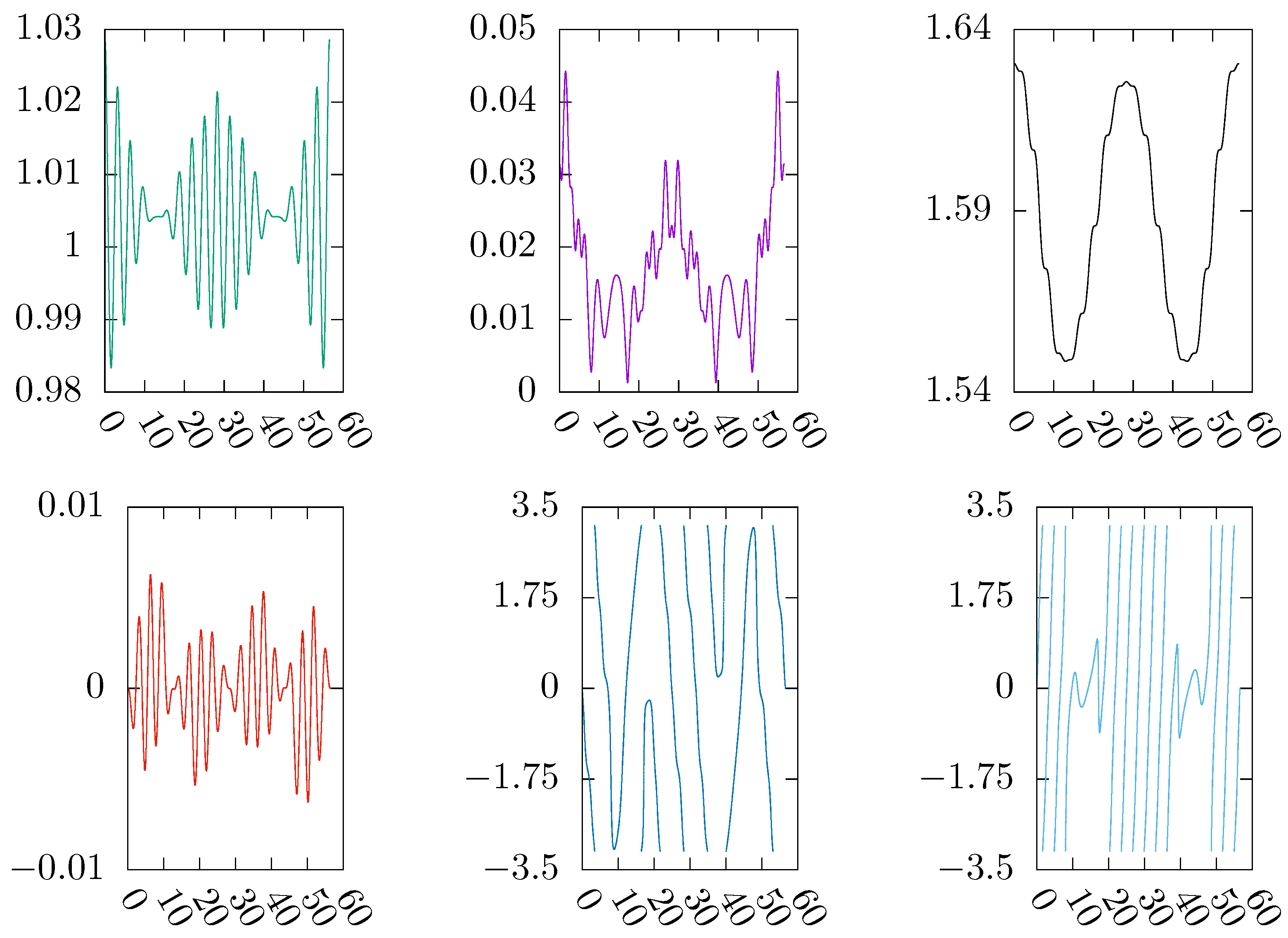
Figure 2.
The orbital elements of a high-altitude, near-polar, near-circular lunar-type periodic orbit in the Moon-Earth elliptic RTBP with . The period is in the scaled time s. The type of the initial values is . The altitude approximates 10170km.
Figure 2.
The orbital elements of a high-altitude, near-polar, near-circular lunar-type periodic orbit in the Moon-Earth elliptic RTBP with . The period is in the scaled time s. The type of the initial values is . The altitude approximates 10170km.
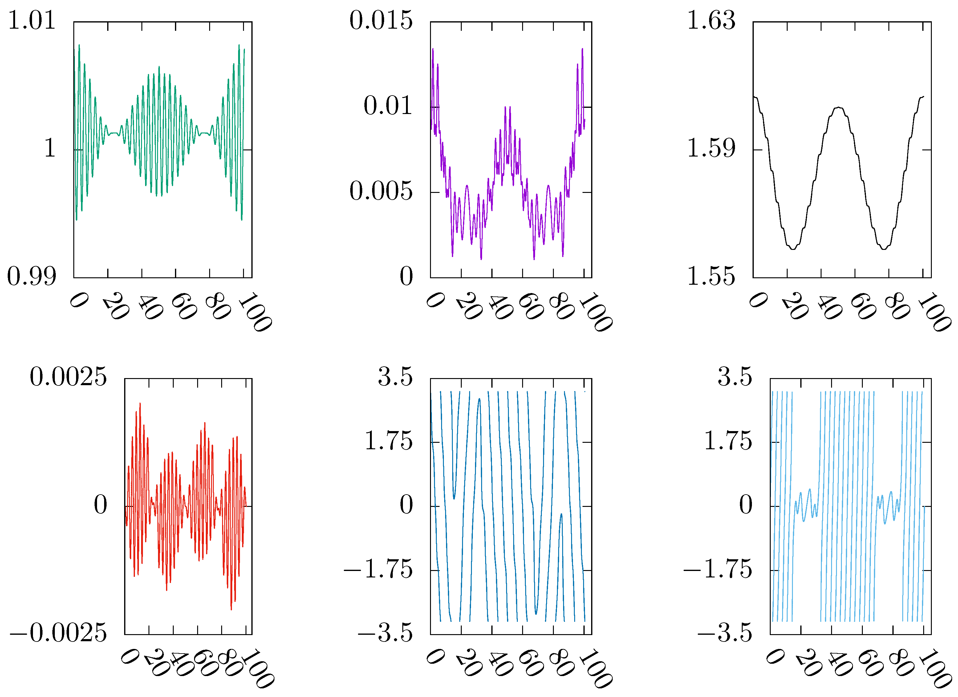
Figure 3.
A high-altitude, near-polar, near-circular lunar-type periodic orbit with . The period is in the scaled time s. The type of the initial values is . The altitude approximates km. The orbit in the scaled Cartesian coordinates is shown in the left graph, and a pair of the Poincaré-Delaunay elements , are drawn in the right graph.
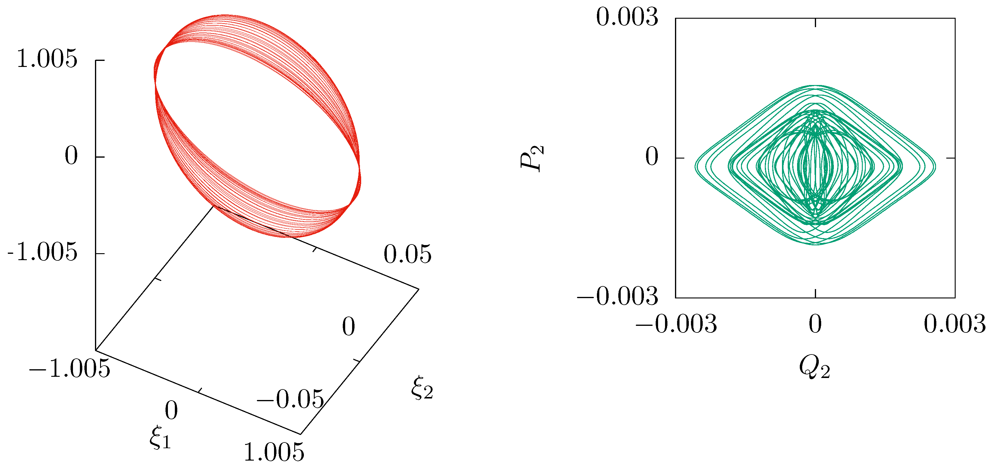
Figure 4.
Lunar inertial coordinate frame and Lunar equatorial rotating frame .
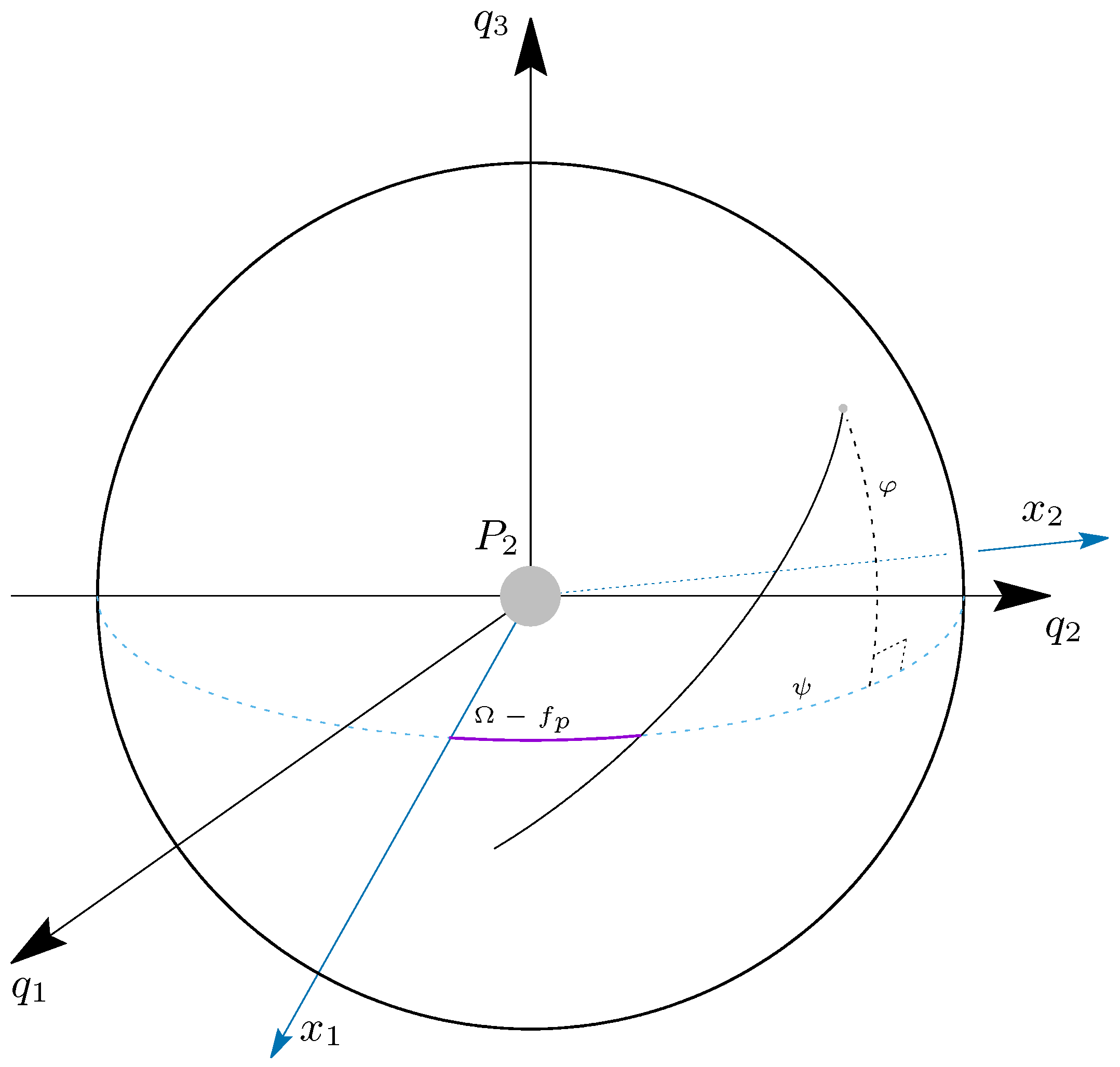
Figure 5.
The orbital elements of a Lunar periodic orbit of "" type with . The altitude is about km.
Figure 5.
The orbital elements of a Lunar periodic orbit of "" type with . The altitude is about km.
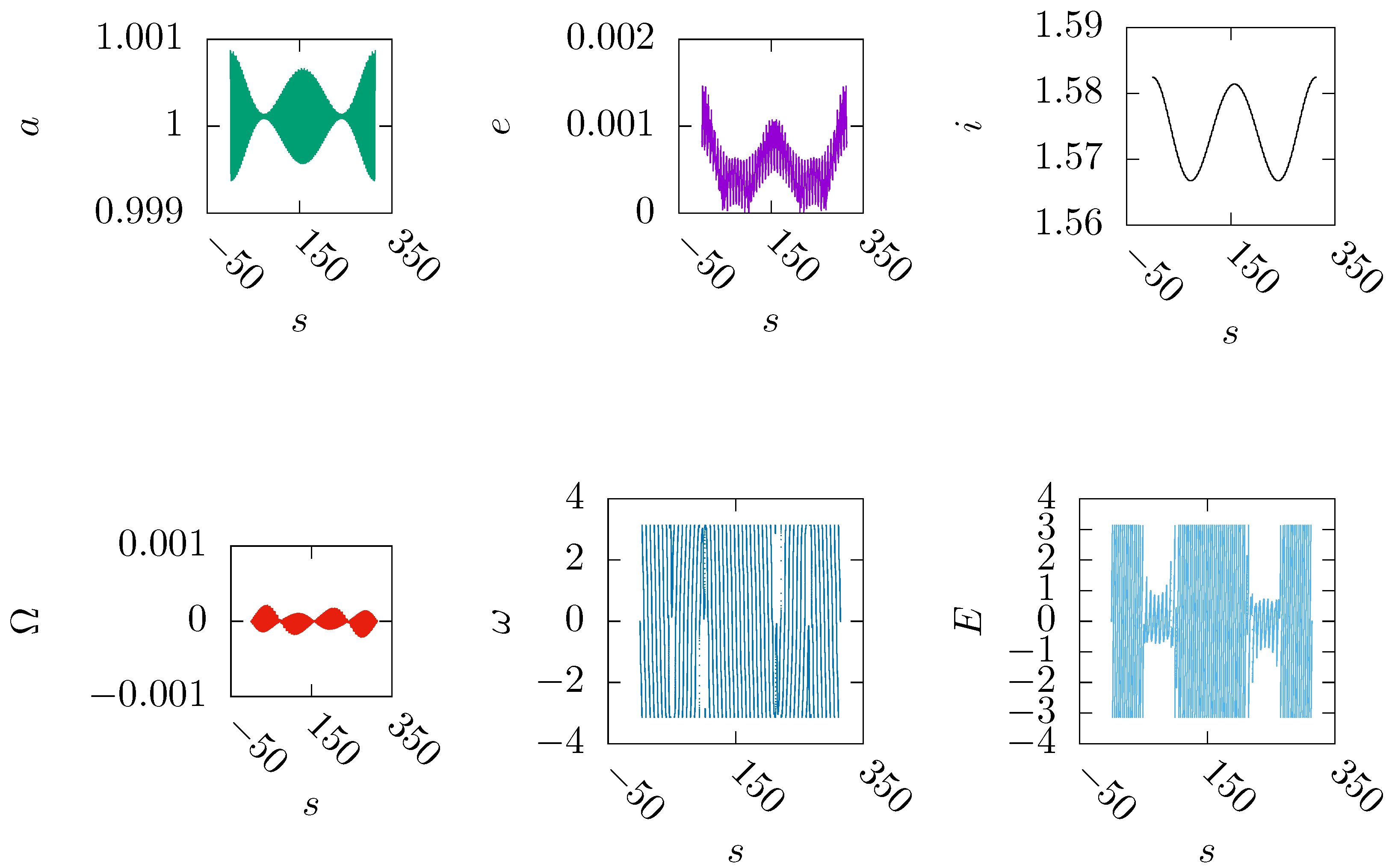
Figure 6.
The orbital elements of a Lunar periodic orbit of "" type with . The altitude is about km.
Figure 6.
The orbital elements of a Lunar periodic orbit of "" type with . The altitude is about km.
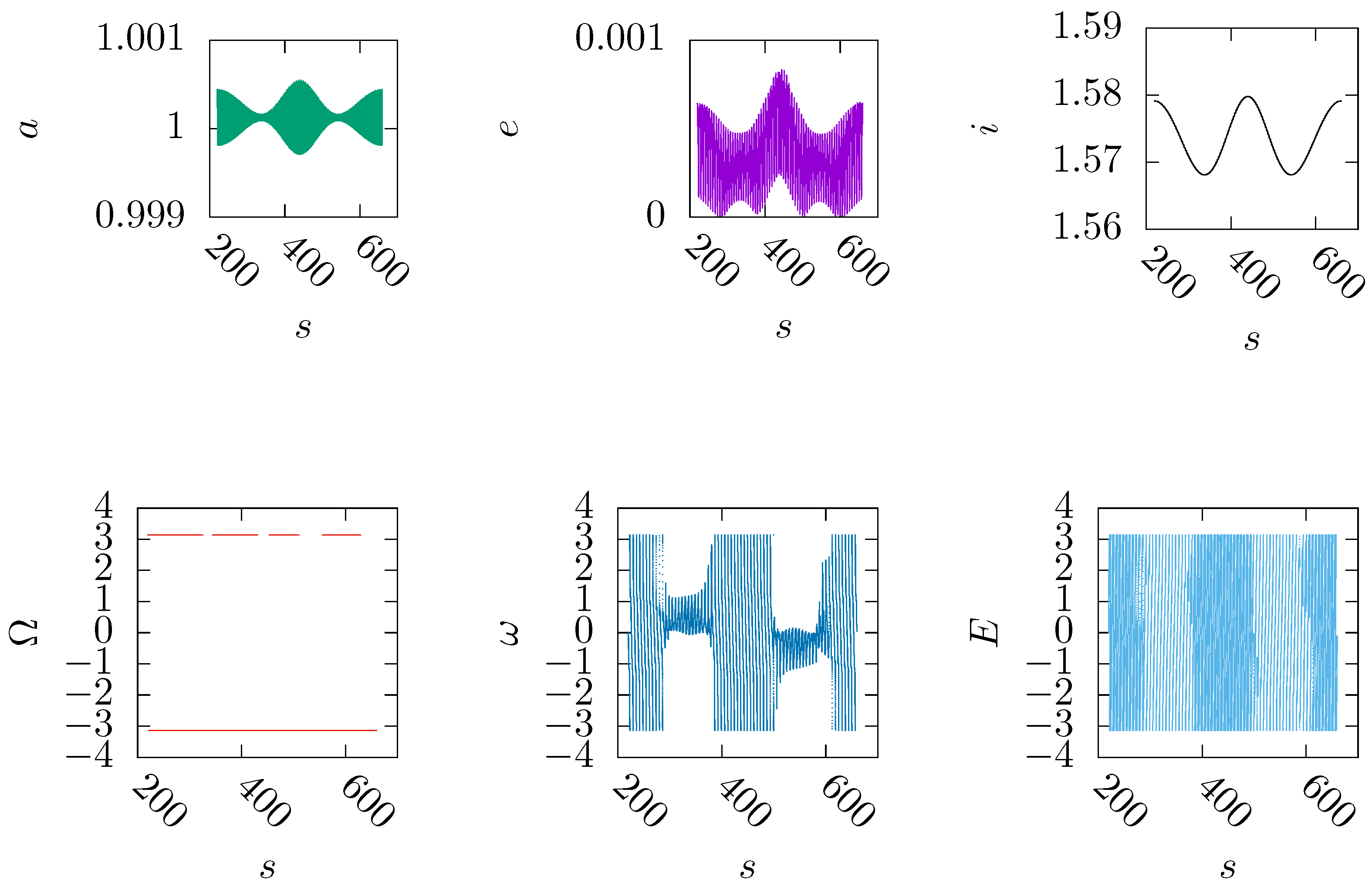

Table 1.
Some initial values of the near-polar, near-circular, lunar-type periodic orbits in the elliptic RTBP.
Table 1.
Some initial values of the near-polar, near-circular, lunar-type periodic orbits in the elliptic RTBP.
| j/k,type1 | |||
| 9/1, | 0.99620440178 | -0.06082772318 | ±1.0157184687 |
| 9/1, | -0.99470649817 | 0.06185840160 | ±1.0154002218 |
| 10/1, | 0.99910153226 | -0.050852737 | ±1.0072154827 |
| 10/1, | -0.99837950690 | 0.0506041258 | ±1.0087412525 |
| 16/1, | 0.99925242695 | -0.035922494 | ±1.0043641526 |
| 16/1, | -0.99851083910 | 0.0360488668 | ±1.0047376373 |
| 36/1, | 1.00010727626 | -0.0146998968 | ±1.0003869346 |
| 36/1, | -0.99974967250 | 0.0147026686 | ±1.0007698831 |
| 37/1, | 0.99999430950 | -0.0157684742 | ±1.0006628074 |
| 37/1, | -0.99962561652 | 0.0157786232 | ±1.0009929915 |
| 50/1, | 1.0000454998 | -1.16852281E-2 | ±1.0003121582 |
| 50/1, | -0.999748470093 | 1.169015346E-2 | ±1.000591975 |
| 50/1, | 1.00010809345 | -1.05990235E-2 | ±1.00014917507 |
| 50/1, | -0.99981879968 | 1.060132171E-2 | ±1.00044900515 |
| 120/1, | 1.000063875 | -4.87551E-3 | ±0.999997510 |
| 120/1, | -0.9999007299785 | 4.8763318183E-3 | -1.000158994073 |
| 150/1, | 1.00005889302967 | -3.900799586228E-3 | 0.99998031895716 |
| 150/1, | -0.99991304641419 | 3.225120713516E-3 | -1.0001276778590 |
1 The types are defined by the signs of .
Table 2.
Some initial values of the near-polar, near-circular, lunar frozen periodic orbits in the elliptic RTBP perturbed by the terms.
Table 2.
Some initial values of the near-polar, near-circular, lunar frozen periodic orbits in the elliptic RTBP perturbed by the terms.
| j/k,type1 | |||
| 38, | 0.999996415501457 | -1.53265760125584E-2 | 1.00063234441343 |
| 38, | 0.999996323959347 | -1.53265221246967E-2 | -1.00063243652928 |
| 38, | -0.999631537537576 | 1.53360715507054E-2 | 1.00096137315743 |
| 38, | -0.999631572957102 | 1.53361607836104E-2 | -1.00096133644985 |
| 38, | 1.00010457611908 | -1.39262375517334E-2 | 1.00034505669525 |
| 38, | 1.00010457613606 | -1.39262375145222E-2 | -1.00034505667884 |
| 38, | -0.999755336066306 | 1.39291300677261E-2 | 1.00071623453464 |
| 38, | -0.999755336071655 | 1.39291298616095E-2 | -1.00071623453208 |
| 50, | 1.00004036237187 | -1.16399095055137E-2 | 1.00032604091855 |
| 50, | 1.00004036442821 | -1.16399055608615E-2 | -1.00032603891154 |
| 50, | -0.999736185844210 | 1.16448719424375E-2 | 1.00061301131761 |
| 50, | -0.999736185751775 | 1.16448718613465E-2 | -1.00061301141084 |
| 50, | 1.00010324877502 | -1.06014270499141E-2 | 1.00016221064751 |
| 50, | 1.00010324742691 | -1.06015693670615E-2 | -1.00016221050752 |
| 50, | -0.999806261225514 | 1.06039245231929E-2 | 1.00046973982848 |
| 50, | -0.999806260045887 | 1.06039241923682E-2 | -1.00046974101071 |
| 50, | 1.00004772495397 | -1.16437280686876E-2 | 1.00031865811095 |
| 50, | -0.999727871097841 | 1.16482584577867E-2 | 1.00062129340388 |
| 50, | -0.999727871210650 | 1.16482585774023E-2 | -1.0006212932898344 |
| 50, | 1.000047724953971 | -1.16437280686877E-2 | 1.00031865811095 |
| 50, | 1.000047723820043 | -1.16437303795379E-2 | -1.00031865921609 |
| 60, | 1.00005445614547 | -9.69443727684011E-3 | 1.00020411562384 |
| 60, | 1.00005445666738 | -9.69443733030811E-3 | -1.00020411510206 |
| 60, | -0.999780858404711 | 9.69780610332384E-3 | 1.00046714423176 |
| 60, | -0.999780830682264 | 9.69781696395454E-3 | -1.00046717183446 |
| 60, | 1.00009836808750 | -8.86151811506304E-3 | 1.00009091857796 |
| 60, | 1.00009836626972 | -8.86152667714532E-3 | -1.00009092031881 |
| 60, | -0.999829057478298 | 8.86344960938257E-3 | 1.00036671317776 |
| 60, | -0.999829058314773 | 8.86344660447464E-3 | -1.00036671236851 |
| 70, | 1.00006122089056 | -8.32258582949308E-3 | 1.00013342805500 |
| 70, | 1.00006122070046 | -8.32258595263936E-3 | -1.00013342824388 |
| 70, | -0.999807148471916 | 8.32518964348363E-3 | 1.00038049962717 |
| 70, | -0.999807149512763 | 8.32518602724036E-3 | -1.00038049861647 |
| 70, | 1.00009370579491 | -7.65010043854636E-3 | 1.00005034663127 |
| 70, | 1.00009370571585 | -7.65010142502368E-3 | -1.00005034670266 |
| 70, | -0.999842137241648 | 7.65183065190509E-3 | 1.00030621538970 |
| 70, | -0.999842137612930 | 7.65182240120627E-3 | -1.00030621508136 |
| 70, | -0.99980224406757 | 8.326726523174E-3 | 1.000385394761 |
1 The types are defined by the signs of .
Disclaimer/Publisher’s Note: The statements, opinions and data contained in all publications are solely those of the individual author(s) and contributor(s) and not of MDPI and/or the editor(s). MDPI and/or the editor(s) disclaim responsibility for any injury to people or property resulting from any ideas, methods, instructions or products referred to in the content. |
© 2025 by the authors. Licensee MDPI, Basel, Switzerland. This article is an open access article distributed under the terms and conditions of the Creative Commons Attribution (CC BY) license (http://creativecommons.org/licenses/by/4.0/).
Copyright: This open access article is published under a Creative Commons CC BY 4.0 license, which permit the free download, distribution, and reuse, provided that the author and preprint are cited in any reuse.


