1. Introduction
Sea surface temperature (SST) plays a crucial role in air–sea interactions and is a key climate factor of global change. Variation in SST has substantial impact on regional climate variability, influencing global precipitation patterns and potentially leading to extreme events such as droughts and floods [
1,
2,
3,
4]. SST short-term fluctuations can be indicative of marine heatwaves, which can have severe impact on marine ecosystems globally [
5,
6,
7,
8,
9]. Short-term SST forecasting is influenced by numerous factors, among which oceanic mesoscale eddies are particularly important. Due to their strong dynamical effects, these eddies can induce extreme short-term SST anomalies. Therefore, understanding and addressing the influence of mesoscale eddies is essential for improving short-term SST forecasting.
In recent years, data-driven deep learning (DL) methods have gained widespread application in ocean and atmospheric sciences due to their ability to learn complex nonlinear relationships, such as eddy identification, downscaling, SST reconstruction, and parameterization of physical processes [
10,
11,
12,
13,
14,
15]. Various types of DL models have been widely explored in SST forecasting. Recurrent neural networks (RNNs), like long short-term memory networks (LSTMs) and gated recurrent units (GRUs), primarily focus on the temporal evolution of SST at individual locations and have been applied to SST forecasting in specific regions [
16,
17,
18,
19]. However, these models struggle to capture complex spatial correlations across areas. Researchers have adopted convolutional neural networks (CNNs) to address this limitation, which leverages their strengths in spatial feature extraction to significantly enhance SST prediction performance [
20]. Residual neural networks (ResNets) further improve model depth by introducing a residual learning framework, effectively mitigating the gradient vanishing problem in deep networks [
21]. Therefore, different types of CNN networks and their variants have also been applied to short-term SST forecasting [
22,
23,
24,
25,
26]. A typical network is Convolutional Long Short-Term Memory (ConvLSTM), which combines the advantages of CNN and RNN, can effectively extract temporal and spatial information, and improve the model's forecast accuracy [
27,
28]. These models have shown significant progress in improving prediction accuracy and reliability.
With the rapid advancement of DL, the Transformer architecture [
29,
30] (see
Appendix A for details) has emerged as a powerful tool across various fields due to its capability to capture long-range dependencies and model complex spatiotemporal relationships. While it has been successfully applied to SST super-resolution tasks [
31], its potential for short-term SST forecasting remains relatively unexplored.
Mesoscale eddies are widely distributed in the ocean and they are the primary drivers of mesoscale SST variability [
32]. These eddies significantly impact SST forecasts, with dynamical forecast models often exhibiting notable errors in eddy-active regions due to their complex dynamics and temperature structures [
33,
34]. These errors are also particularly pronounced over eddy-active areas [
35,
36,
37] in the simulations of the High-Resolution Ocean Model Intercomparison Project. Studies on quantifying short-term SST forecast errors and their spatial distribution in eddy-active regions remain limited. Furthermore, forecasting short-term SST anomalies caused by eddies has received little attention as previous DL researches have concentrated on forecasting sea surface height associated with eddies [
38,
39,
40].
This study introduces an innovative Transformer-based variant, the U-Transformer model, to improve short-term global SST forecasting. The U-Transformer model is designed to capture spatial and temporal features simultaneously, enabling more accurate multi-step forecasts for the coming days. In this study, we compare the performance of the U-Transformer model with two classic CNN-based model types—ConvLSTM and ResNet—across global areas and regions with active mesoscale eddies. The paper is organized in the following.
Section 1 provides an introduction.
Section 2 describes the data and methods.
Section 3 presents the results.
Section 4 contains discussion and conclusions.
2. Data and Methods
2.1. Data
The data used in this study is derived from the NOAA/NESDIS/NCEI Daily Optimum Interpolation Sea Surface Temperature (OISST), version 2.1, dataset, as detailed in [
41,
42]. This dataset provides global SST observations with a spatial resolution of 0.25° and a daily temporal resolution, covering the period from January 1, 1982, to December 31, 2022. The global coverage spans from 89.975°S to 89.875°N and from 0.125°E to 359.875°E.
OISST v2.1 integrates SST measurements from satellite observations (e.g., AVHRR), in-situ measurements from ships, drifting buoys, and Argo floats. These data sources are blended using an optimum interpolation algorithm, which ensures consistency and accuracy through bias adjustments based on in-situ observations. The interpolation leverages spatial autocorrelation and temporal consistency to generate a high-resolution, gridded SST product.
While OISST v2.1 provides high global accuracy, regions with sparse in-situ observations—such as the Indian, South Pacific, and South Atlantic Oceans—rely more heavily on satellite data and interpolation, which may lead to higher uncertainties. However, v2.1 improvements, including bias corrections, incorporation of Argo data above 5m depth, and enhanced Arctic SST estimates, have significantly reduced these biases and improved overall accuracy.
To evaluate the SST forecasts, we employed data from three prominent oceanographic research programs: the Tropical Atmosphere Ocean (TAO) project, the Research Moored Array for African–Asian–Australian Monsoon Analysis and Prediction (RAMA) project, and the Prediction and Research Moored Array in the Tropical Atlantic (PIRATA) project. These programs utilize moored buoys that provide essential real-time data on oceanic and atmospheric conditions.
All three arrays provide data daily, measuring key parameters such as SST, air temperature, wind stress, 10m wind speed, and longwave radiation. The spatial resolution of these arrays is approximately 2° latitude by 10° longitude, with the TAO array covering the equatorial Pacific, RAMA covering the tropical Indian Ocean, and PIRATA covering the tropical Atlantic Ocean.
This study employed the spatial filtering methods of [
43] and [
44] to extract the ocean mesoscale signal. A filter box with dimensions of 3° in both longitude and latitude was used to calculate the mean value within the box, which comprised the low-pass filtered value representing the large-scale signal. The difference between the original SST and the low-pass filtered value was then utilized to isolate and reflect the role of the mesoscale signal.
2.2. Model
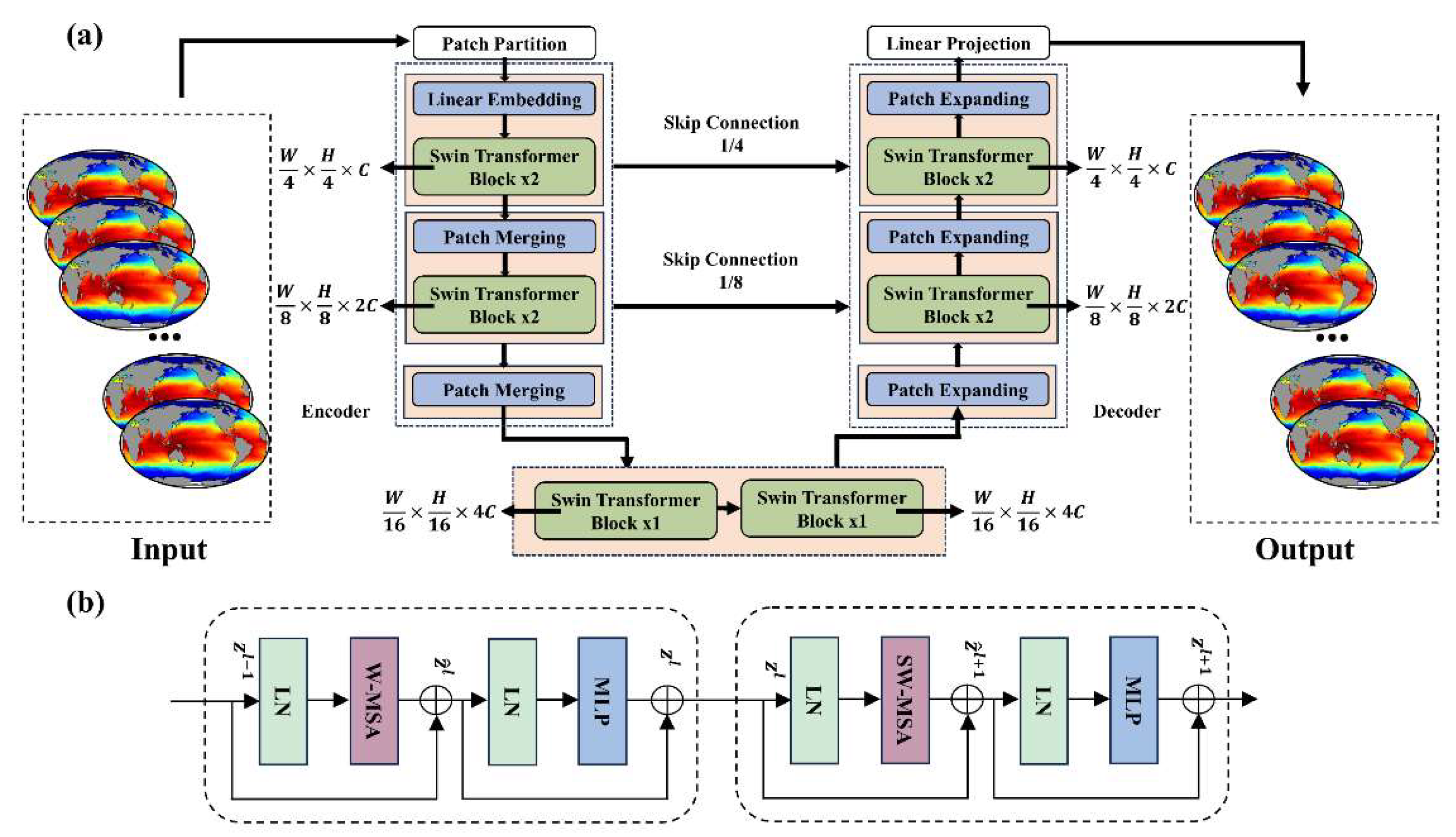
The proposed U-Transformer architecture eliminates convolutional and recursive operations, replacing them with a self-attention mechanism to extract multivariate relationships in parallel, regardless of spatial and temporal distance. The U-Transformer, as shown in
Figure 1a, comprises an encoder, decoder, and skip connections [
45], and was built on the Swin Transformer module [
46]. The Swin Transformer module employs self-attention within nonoverlapping local windows to reduce network complexity and build hierarchies for multiscale feature extraction.
The encoder starts by dividing the input SST field into 4 × 4 non-overlapping patches, each with a feature dimension These patches are then projected to an arbitrary dimension C (e.g., C=96) through a linear embedding layer, reducing both the spatiotemporal dimensions and memory usage. The resulting matrix has dimensions (, where and represent the height, and width dimensions of the input.
These encoded patches pass through a series of Swin Transformer Blocks and a patch merge layer. The patch merge layer reduces the spatial dimensions by half while doubling the feature dimension, enabling hierarchical feature representation. For instance, after the first patch merge layer, the matrix dimensions become (.
Similarly, the decoder employs Swin Transformer Blocks and a patch expand layer. The patch expand layer upsamples the feature mappings to restore the spatial dimensions progressively. For example, the dimensions change from ( back to (. Skip connections from the encoder provide contextual features to the decoder, mitigating spatial information loss. Finally, a linear projection layer converts the output of the decoder into the desired shape, , to generate the future SST field forecast.
A key innovation is the shifted window-based multi-head self-attention (SW-MSA) module in the Swin Transformer, which addresses the lack of cross-window connectivity in a standard window-based MSA. The SW-MSA alternates between two partitioning configurations, with each Swin Transformer Block comprising an SW-MSA, a 2-layer multilayer perceptron (MLP) with Gaussian Error Linear Unit activation, Layer Normalization (LN), and residual connections (
Figure 1b). This process can be formulated as follows:
where
and
denote the output features of the (S)W-MSA module and the MLP module for block l, respectively. The self-attention is computed as follows:
where
are the query, key, and value matrices, respectively,
is the query/key dimension, and
is the number of patches in a window.
2.3. Implementation Details
After the data is preprocessed through normalization, land locations are assigned a value of 0 to exclude them from the model's predictions. Subsequently, the generated input-output pairs are segmented along the time axis, with each input sample comprising the SST data from the previous ten days and the corresponding output representing the SST data for the next ten days. This allows the model to capture the temporal dependencies within SST patterns and predict future values. The dataset is then split into training, validation, and test sets. Data from 1982 to 2019 are used for training and validation, with 90% allocated to training and 10% reserved for validation. The model is trained using this split, with the validation set utilized for hyperparameter tuning to prevent overfitting. Finally, data from 2020 to 2022 are retained as an independent test set, enabling a robust evaluation of the model's performance on unseen data. During model evaluation, a spatial filtering method is applied to isolate mesoscale and large-scale signals, ensuring a comprehensive assessment of the model's forecasting ability.
The model was trained using a latitude-weighted L2 loss function, which accounts for the area of grid points across different latitudes. To improve training efficiency and model stability, inputs and outputs were normalized using zero-mean normalization.
Our weighted L2 loss function can be expressed as:
where
is the true value,
is the predicted value,
is the latitude of the corresponding point, and
is the latitude-based weight.
Our zero-mean normalization function can be expressed as:
where
is the original data,
is the mean of the feature,
is the standard deviation of the feature,
is the normalized data. The mean and standard deviation values are computed based on the historical dataset spanning from 1982 to 2019.
All models were implemented using the PyTorch framework and trained on a cluster of 16 nodes, each with two accelerator cards (16 GB memory). The training process ran for 100 epochs, with a batch size 2 per card. We used the AdamW [
47,
48] optimizer, as it is known for its effectiveness in stabilizing training in deep learning models. The optimizer parameters, β₁ = 0.9 and β₂ = 0.95 were chosen based on their widespread use in similar tasks, which balances gradient momentum and stability. An initial learning rate of
was applied, as it provided a good balance between convergence speed and performance during preliminary tests. Additionally, we used a weight decay of 0.1 to mitigate overfitting, ensuring generalization. All training parameters were kept consistent across models to maintain fairness and comparability.
We compared the proposed U-Transformer model with ConvLSTM and ResNet models, using the same input-output structures and preprocessing across all models. The ConvLSTM architecture was adapted from [
49], while the ResNet model was based on ResNet-18 [
21]. The parameter details of ConvLSTM and ResNet can be seen in
Appendix B. All forecasts were derived from the test set, ensuring consistent methodology across models.
2.4. Evaluation Methods
We evaluated the forecast performance using the area-weighted RMSE, Bias, and anomaly correlation coefficient (ACC), which were calculated as follows:
where
is the forecast initialization time in testing set
and
is the forecast lead time step added to
;
are the number of time steps and the grid points in the latitude and longitude directions, respectively;
represents the weights of different latitudes;
are the forecast field and the true field at time
, respectively; and
represents the climatological mean calculated using data from 2000–2010.
3. Results
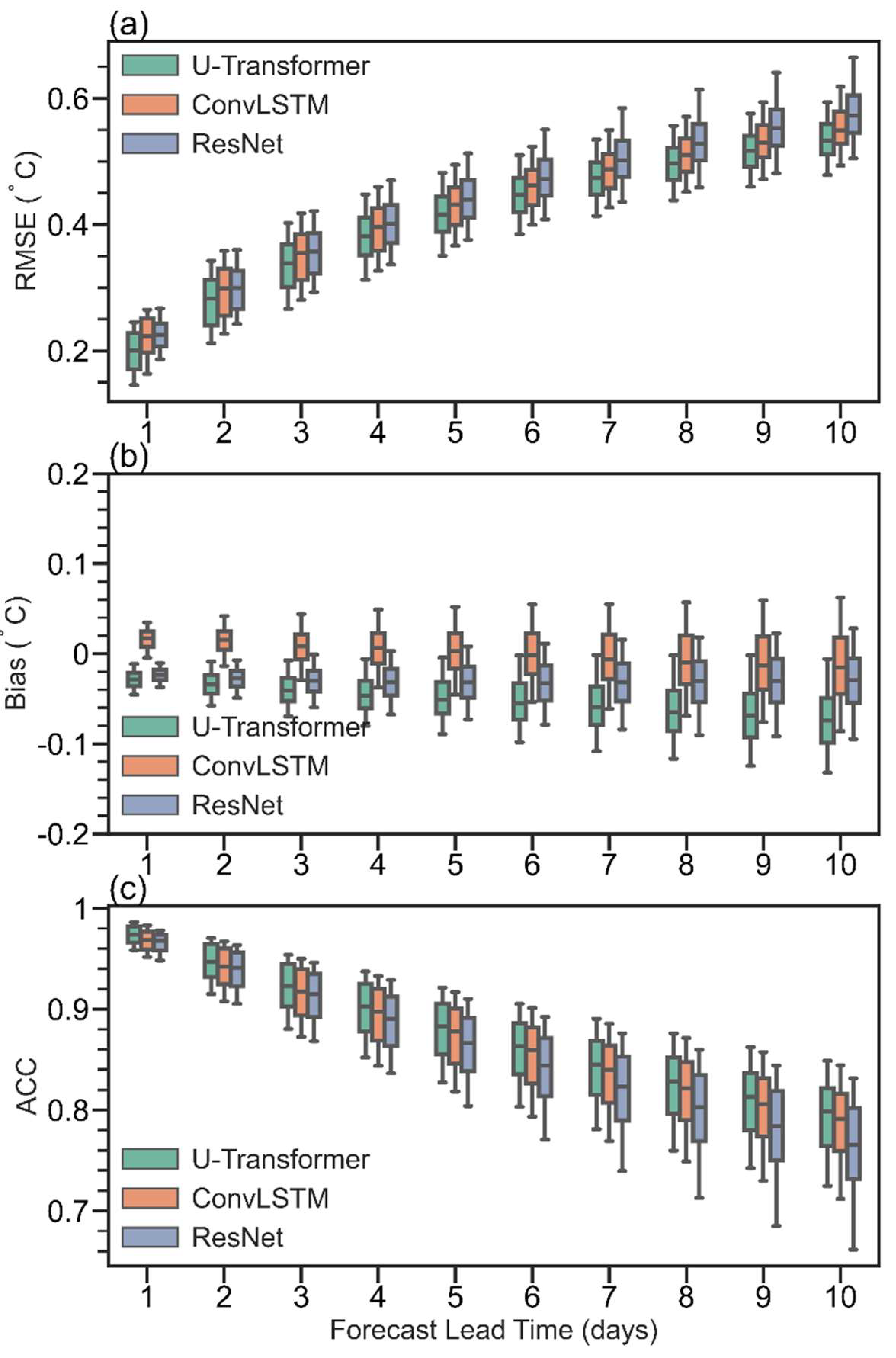
The U-Transformer model has good ability to forecast short-term global SST. The global average RMSEs produced by the U-Transformer model are in the range 0.2–0.54 °C from 1- to 10-day lead times during 2020–2022 (
Figure 2a), demonstrating its consistent accuracy. At the 5-day lead time, the U-Transformer model achieves a global RMSE of 0.42 °C, slightly outperforming the ConvLSTM and ResNet models that have RMSEs of 0.43 and 0.44 °C, respectively. Although the RMSEs increase with increasing lead time for all three models, the U-Transformer model maintains the lowest RMSE values consistently for all (from 1- to 10-day) lead times. Meanwhile, the smaller RMSEs for all grid points (spread of RMSEs) are achieved in the ConvLSTM and U-Transformer models than those in the ResNet model from 4- to 10-day lead times. According to previous studies, dynamical forecast models have RMSEs of forecasted SSTs of approximately 0.35–1.1 °C at the 1-day lead time [
50] with the smallest forecast SST from Met Office Forecast Ocean Assimilation Model (FOAM) dynamical forecast system [
51,
52]. For example, in the LICOM Forecast System v1.0 [
53], the global averaged RMSE of forecasted SST is 0.45–0.55 ℃ at the 1-day lead time. Compared with the RMSEs of SST forecasted by dynamical models, the U-Transformer model can substantially reduce the global SST forecast errors. The RMSE of forecasted SST produced by the model presented by [
27] at the 1-day lead time is 0.27 °C, which is larger than that of the three models built in this study, particularly the U-Transformer model. The above analysis indicates that the U-Transformer model is a good model for forecasting short-term SST globally because it produces the smallest global averaged RMSEs.
The good ability of the U-Transformer model to forecast short-term global SST is also represented in the small biases and large ACC (
Figure 2b and 2c). Generally, all three models exhibit small biases (<0.1 °C) in global averaged SST, although the biases among the three models differ slightly. The U-Transformer model exhibits a cold bias of 0.03–0.06 °C at 1- to 10-day lead times. The ResNet model shows a relatively stable cold bias of approximately 0.02 °C, whereas the ConvLSTM model transitions from a slight warm bias to a cold bias over the same period but with a larger spread of values. The consistency in the sign of the global averaged SST bias for all lead times implies that systematic bias exists for the U-Transformer and ResNet models, which requires further study. The U-Transformer model consistently achieves the largest ACC values, starting at approximately 0.97 at a 1-day lead time and gradually decreasing to 0.79 at the 10-day lead time. Meanwhile, the spreads are smaller for the U-Transformer and ConvLSTM models, implying consistently large ACCs and thus, high forecast skill.
The above analysis highlights the reasonable ability of the U-Transformer model to forecast short-term SST globally, outperforming both the ConvLSTM and the ResNet models in terms of forecast error and forecast skill from the perspective of global statistics and the 1- to 10-day lead times.
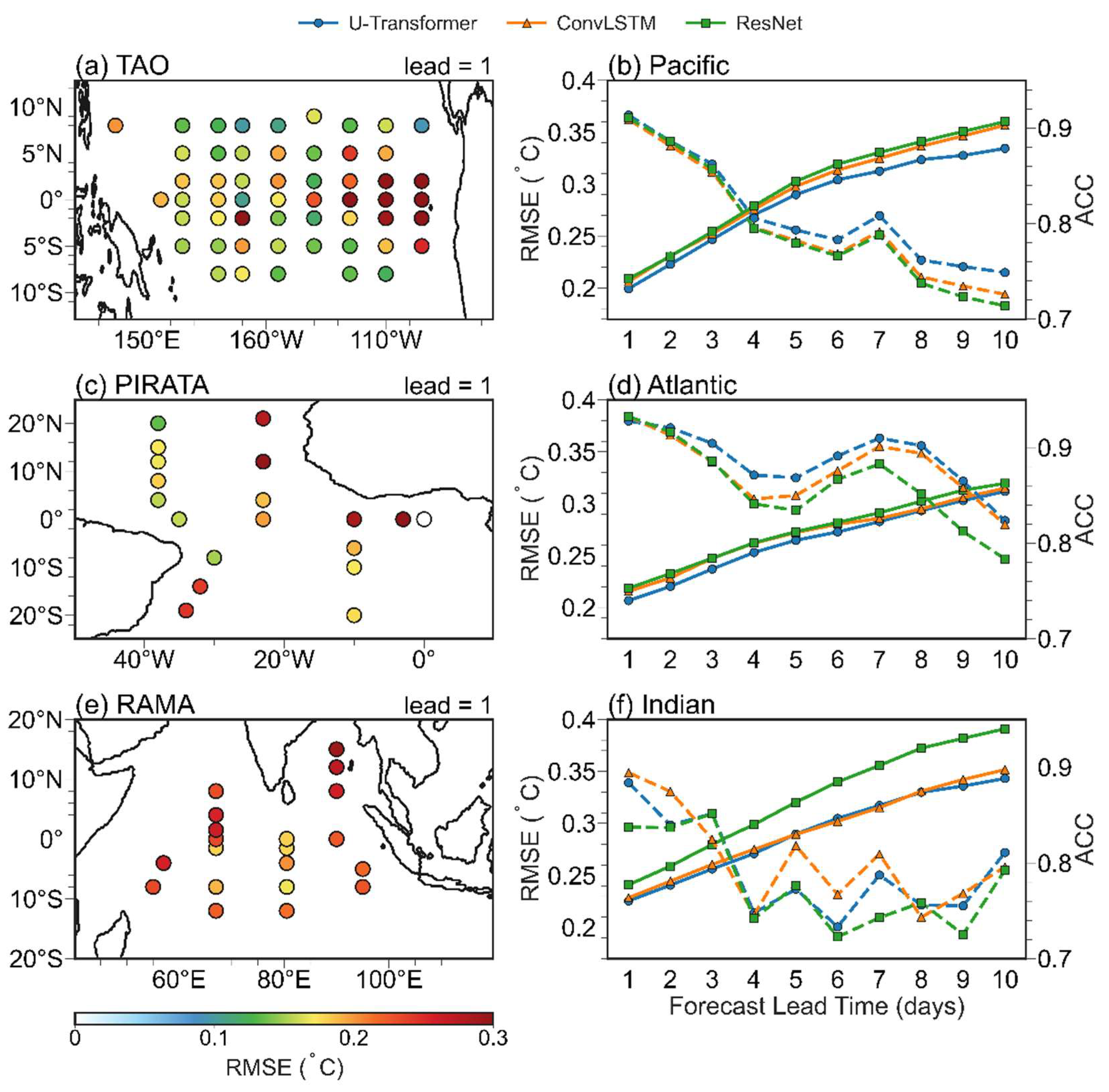
Statistical analysis was also performed for the tropics and the regions with active mesoscale eddies. In the tropical and subtropical oceans, the RMSEs are relatively low and generally do not exceed 0.2 °C, except in the eastern equatorial Pacific (
Figure 3a), which is a region characterized by the Tropical Instability Wave (TIW). In this area, RMSEs exceed 0.3 °C, consistent with the findings of previous studies [
23,
54], and highlighting the challenges in forecasting daily SST changes in the TIW region. In the Atlantic and Indian oceans, higher RMSEs (calculated using observed data from moored stations) are observed in the northeast, while smaller RMSEs (<0.2 °C) are found in the western Atlantic (
Figure 3c). The Indian Ocean exhibits a relatively uniform distribution of RMSEs, with values generally exceeding 0.25 °C (
Figure 3e). In the Pacific Ocean, RMSEs are distributed unevenly, with higher values in the eastern equatorial region and lower values in the western parts (
Figure 3a). Overall, the anomaly correlation coefficient (ACC) decreases as the forecast lead time increases, with the U-Transformer model demonstrating the largest correlation forecast in the Pacific and Atlantic regions (
Figure 3b, d). On the first forecast day, the ACC is approximately 0.9, with the Atlantic region showing the best correlation performance. Interestingly, the ACC does not exhibit a strictly monotonic decrease as the forecast lead time extends, which may be attributed to the limited number of observed samples available for evaluation. It is evident from
Figure 2 and
Figure 3 that the U-Transformer model can substantially reduce forecast errors relative to those of the ConvLSTM and ResNet models, particularly in the TIW region, which is a region with complex oceanic activities and notable regional interactions. The ConvLSTM and ResNet models both struggle to capture these varied regional dynamics because of the use of convolutional networks, whereas the self-attention mechanism in the U-Transformer model might effectively capture the remote dependencies and intricate spatial patterns, making it particularly suited for SST forecasts in such complex regions.
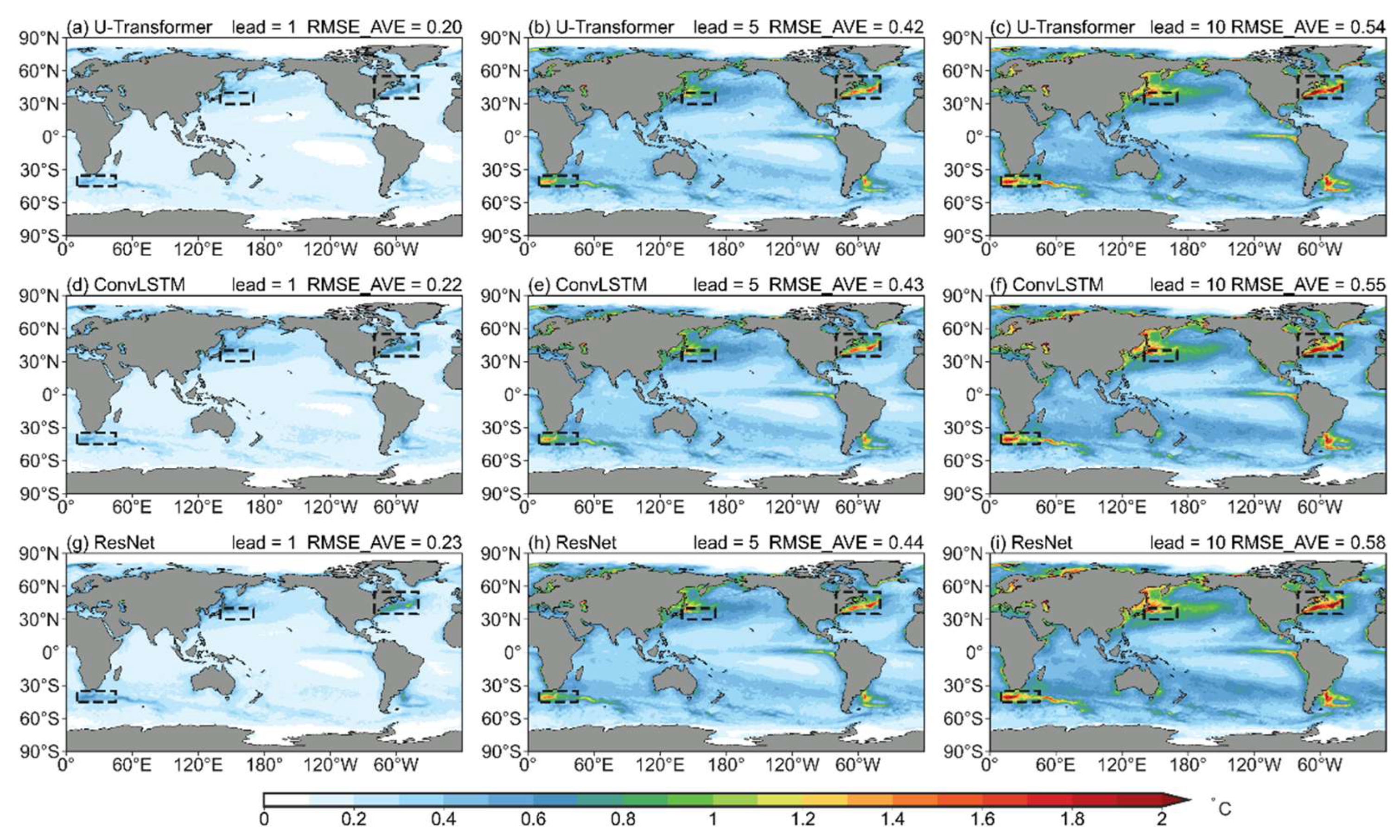
Figure 4 illustrates the spatial RMSE distribution for forecast SST at different lead times (days) in the test set. At the 1-day lead time, the U-Transformer model performs exceptionally well with a global area average RMSE of 0.2 ℃ (
Figure 4a). In the U-Transformer model results, small RMSEs are found mainly in tropical or subtropical ocean areas, whereas large RMSEs are found in regions with active mesoscale eddies. The ConvLSTM and ResNet models can also reproduce the observed SST distribution in the 1-day lead time forecast with RMSE values (0.22–0.23 ℃) slightly larger than those of the U-Transformer model (
Figure 4d, g). As the forecast lead time increases, the forecast error also grows. When forecasting 10 days, the U-Transformer achieves a global average RMSE of 0.54°C, compared to 0.55°C for ConvLSTM and 0.58°C for ResNet (
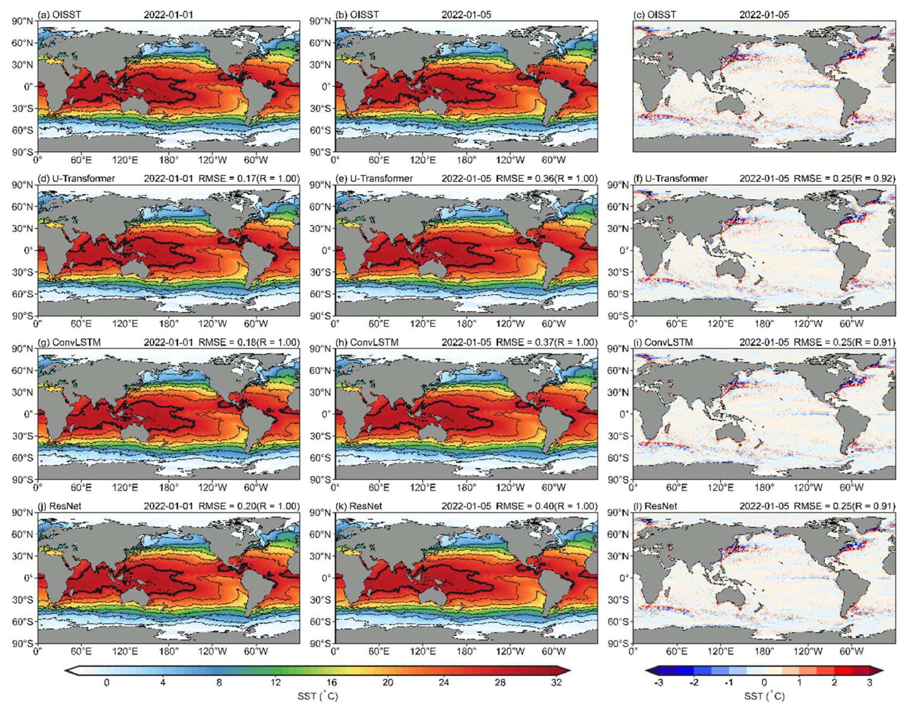
Figure 4c, f, i). Notably, forecast errors are more pronounced in regions with active mesoscale eddies than in other areas. The observed large-scale features of the SST distribution can also be well reproduced on January 1, 2022 at 1- or 5-day lead times by the three DL models (
Figure 5a, d, g, j), such as warm SST in the tropics, cold SST at high latitudes (Arctic Ocean and Southern Ocean), the Indo-Pacific warm pool, and the cold tongue in the equatorial eastern Pacific (
Figure 5b, e, h, k). It is evident that while different models successfully capture the general characteristics and spatial morphology of mesoscale signals, their errors remain significant. The forecast error for mesoscale processes accounts for approximately 70% of the total error, highlighting the complexity of mesoscale activities as a primary contributor to inaccuracies in SST forecasts. Among the evaluated models, the RMSE is consistently around 0.25; however, the U-Transformer model demonstrates superior correlation performance, achieving the largest value of 0.92 (
Figure 5c, f, i, l).
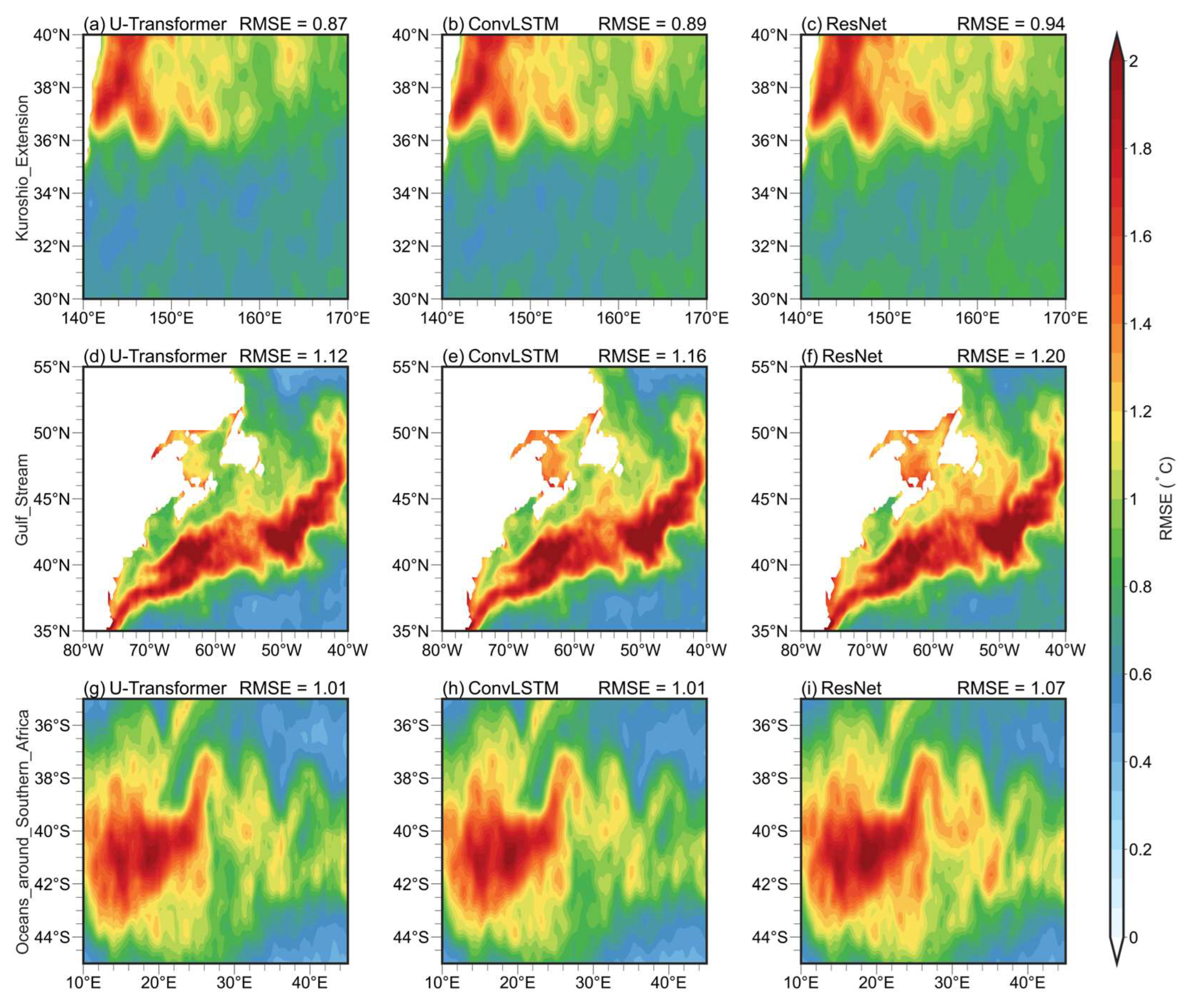
In regions with active mesoscale eddies, the RMSEs are large and the behavior of the forecasted local SSTs requires investigation. The Kuroshio Extension (KE), Gulf Stream (GS), and the oceans around Southern Africa (OSA) are regions chosen to characterize these areas with active mesoscale eddies. In these regions, all three DL models exhibit large RMSEs compared with the global average, particularly within the black dashed boxes shown in
Figure 4 (details as
Figure A1), with errors exceeding 0.6 °C for 1-day lead time forecasts. Additionally, the mesoscale pattern correlation coefficients of the forecasted SSTs are notably lower than those for large-scale patterns, highlighting the challenges in forecasting SST changes associated with mesoscale eddies (
Figure 5).
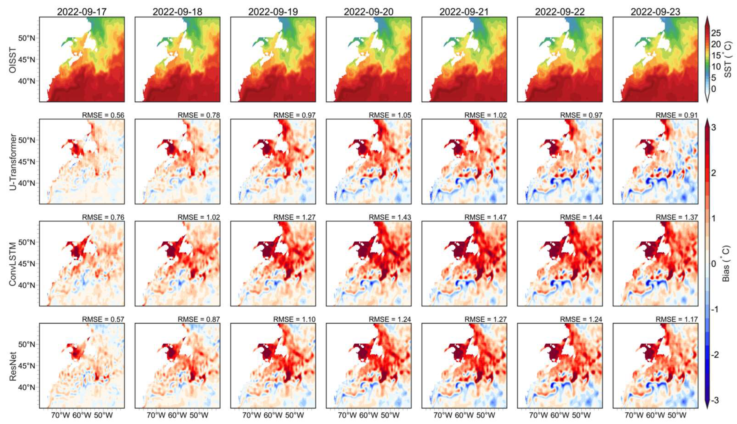
The forecast of a specific day further reflects the ability of SST to forecast in complex ocean regions. The KE was chosen to display the forecast SST evolution in the eddy-active areas.
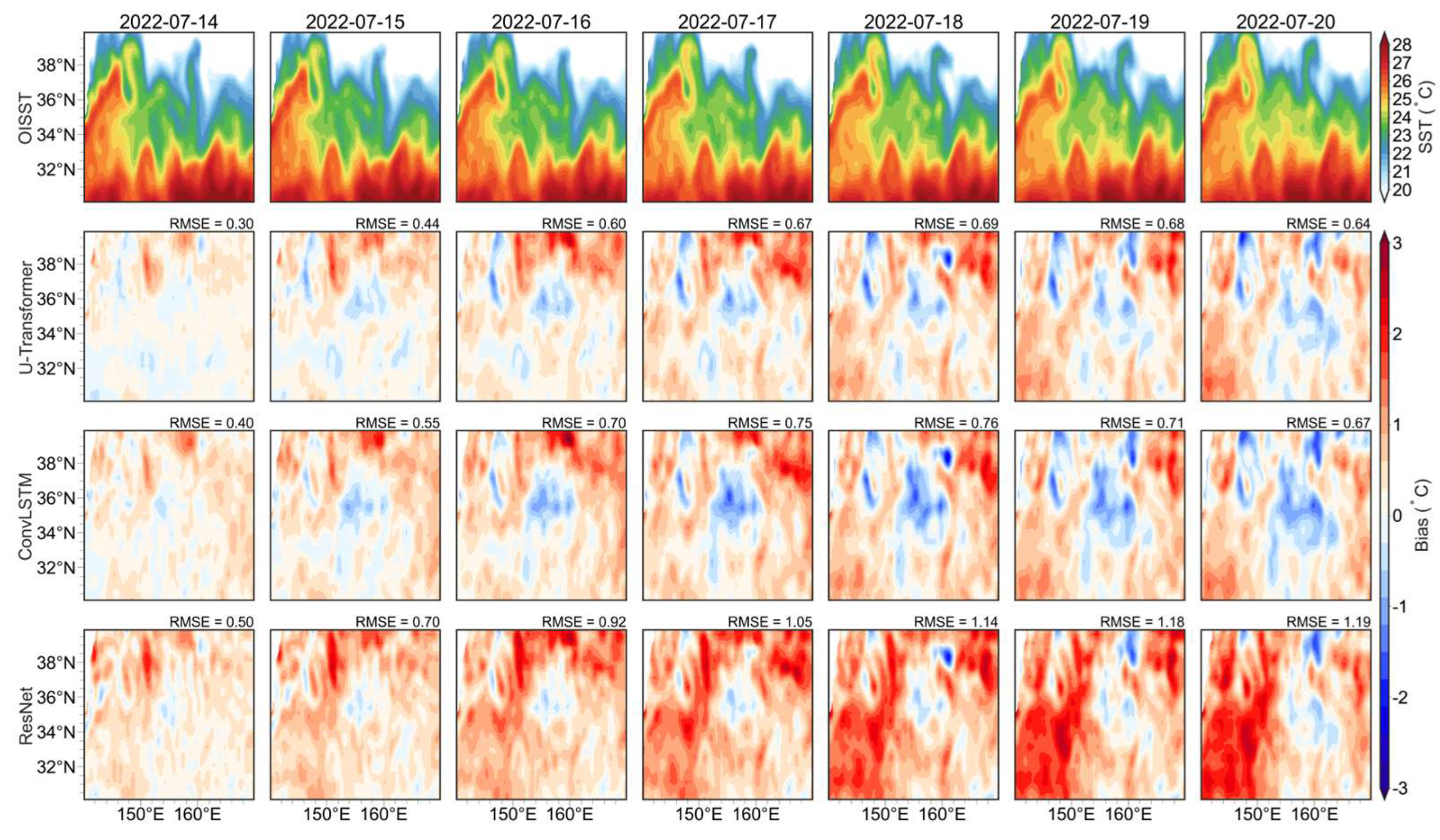
Figure 6 presents the observed OISST SST and daily SST forecast biases in this region from July 14 to July 20, 2022, based on initial conditions from OISST on July 14, 2022. The results demonstrate that DL models effectively capture the overall spatial distribution of SST. The U-Transformer model exhibits smaller biases at the 1-day lead time (July 14, 2022) than the ConvLSTM and ResNet models. South of 36°N, the absolute SST biases are less than 0.3°C, while between 36°N and 39°N, biases exceed 0.5°C in all models at the 1-day lead time. The U-Transformer achieves an RMSE of 0.3°C, outperforming the ConvLSTM (0.4°C) and ResNet (0.5°C) models. The forecast biases become large as the lead times increase. Since the lead times of 4 days, biases south of 36°N become comparable to those north of 36°N in the U-Transformer model. The RMSEs of forecast SST at all lead times are smaller using the U-Transformer model than those using the ConvLSTM and ResNet models, with a slight difference compared to the ConvLSTM model and a larger difference compared to the ResNet model. All models exhibit common biases around finer-scale SST features, particularly near extreme local high or low SST values linked to mesoscale and submesoscale eddies. From 1-day to 3-day lead times, the RMSEs increase significantly, from 0.3 to 0.6°C using the U-Transformer model. Similar evolution behaviors are found in the other two models. This may be caused by the eddy movement and their nonlinear behaviors. Similar patterns of large forecast SST biases and their evolution are evident in the GS and the OSA, as shown in
Figure A2 and
Figure A3. Therefore, the advanced DL models exhibit better capabilities for forecasting SST in eddy-active regions. Further optimization is required to enhance their accuracy and reliability when addressing complex ocean processes, like eddy-rich regions.
Figure 7 and
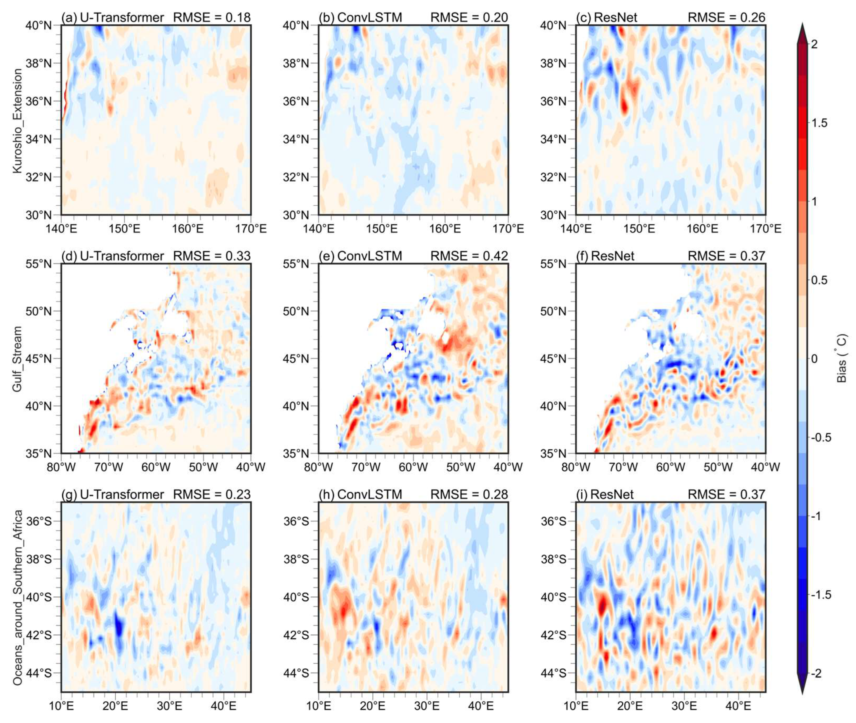
Figure 8 illustrate the spatial distributions of forecast SST biases for the U-Transformer model, selected based on the 10th percentile (lower RMSE) and 90th percentile (higher RMSE) of sorted RMSE values in ascending order. The error distributions across the three DL models are generally consistent under various forecast initial conditions, reflecting the inherent physical characteristics of SST variations in eddy-active regions. However, notable differences in bias magnitudes are observed among the models. In the KE region, the SST bias from the U-Transformer model is predominantly below 0.2°C (
Figure 7a), which is 10-30% smaller than those produced by the ConvLSTM and ResNet models. In contrast, the GS region exhibits significantly more irregular SST bias structures (
Figure 7d-f), resembling features associated with eddies. In this region, the RMSEs are 40-50% larger than those in the KE region for the same model. Similarly, eddy-related bias patterns are evident in the OSA (
Figure 7g-i) but much more obvious in the ConvLSTM and ResNet models. In this area, the RMSEs of the ConvLSTM and ResNet models are 22-61% larger than those of the U-Transformer. While biases in this region are larger than those in the KE, they remain smaller than those in the GS for the same model. These comparisons across different areas indicate the challenges posed by active eddies, which can induce significant forecast SST biases due to their complex capture dynamics.
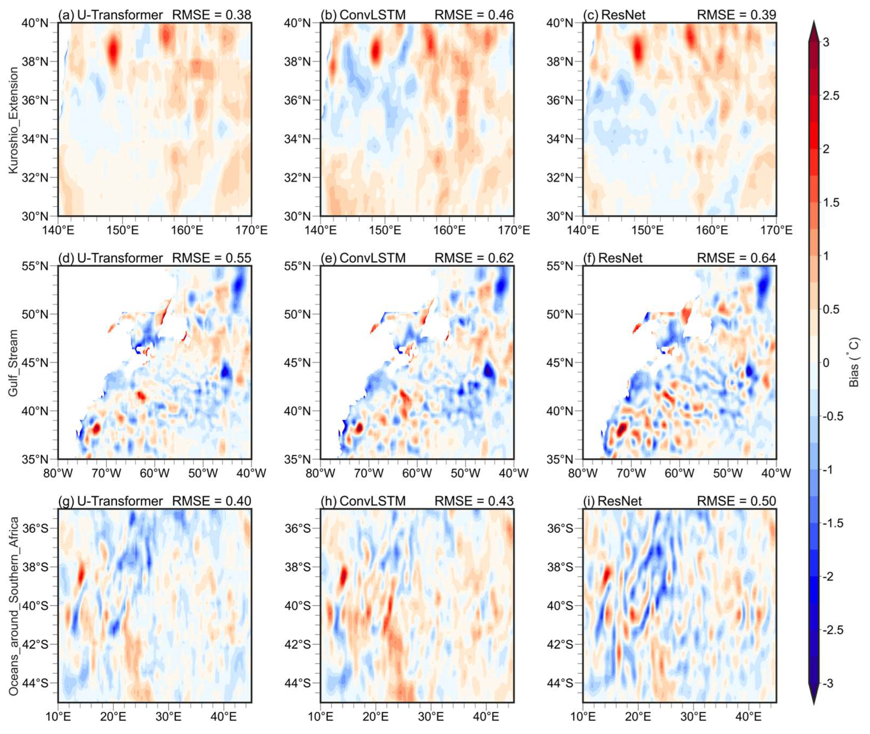
In the cases of larger RMSEs (
Figure 8), larger biases exist for the same region and the same DL model compared with those in the case of smaller RMSEs (
Figure 7). Even under these cases, the U-Transformer model demonstrates smaller SST biases than the ConvLSTM and ResNet models, but the differences vary by region and model. In the KE region, the U-Transformer achieves RMSE reductions of 17% and 3% compared to ConvLSTM and ResNet, respectively. In the GS region, the RMSEs for the U-Transformer are 11-14% smaller than those of the other two models. In the OSA, the U-Transformer reduces RMSEs by 7% compared to ConvLSTM and by 20% compared to ResNet. While the U-Transformer consistently outperforms the other models, the relative improvements are smaller in the larger RMSE case. The above results may be related to much more apparent eddy structures in
Figure 8 than in
Figure 7. These intensified mesoscale eddies significantly influence SST forecasts, highlighting the challenges of accurately capturing such complex dynamics.
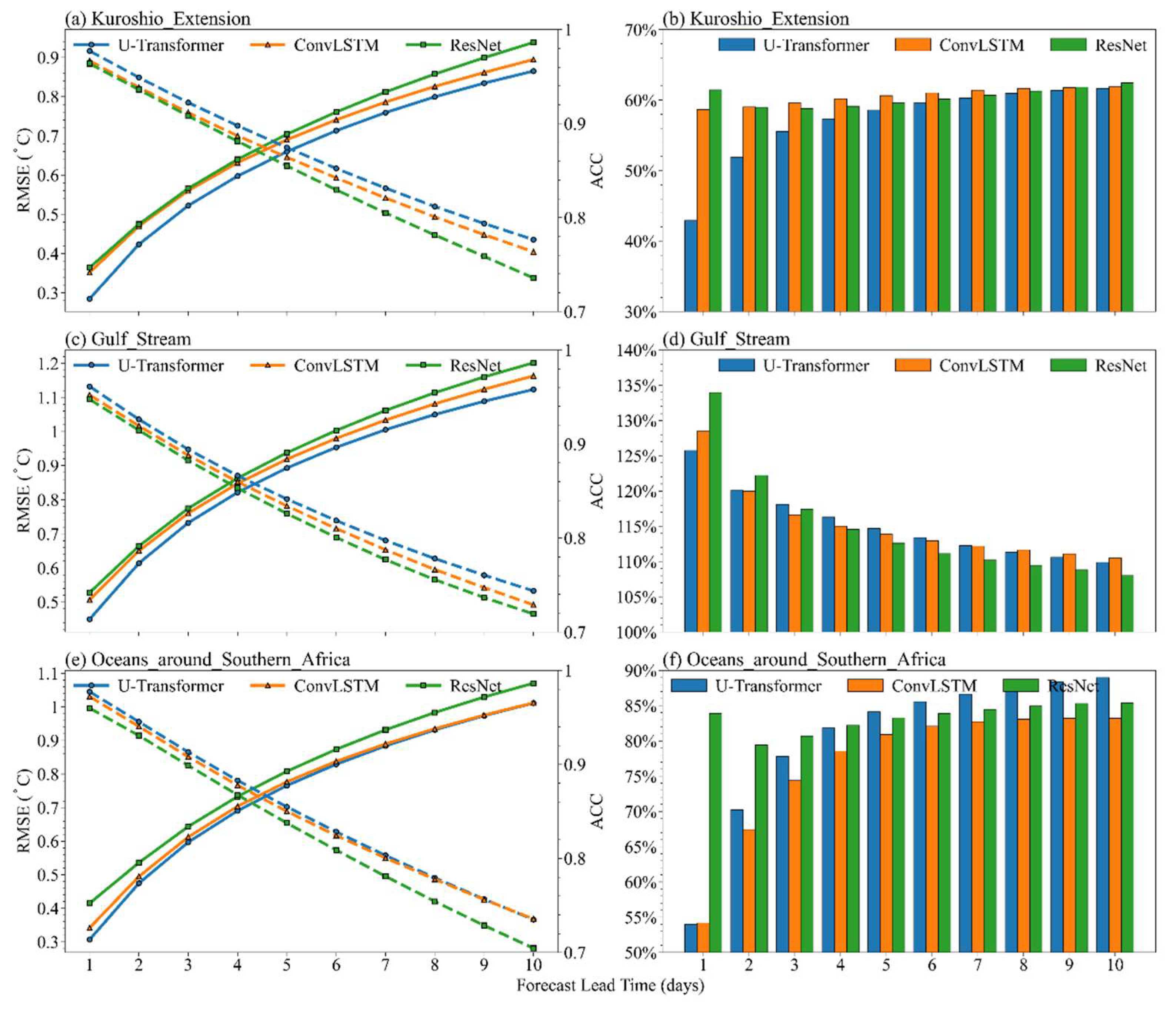
Statistical analysis of these ACC and RMSEs in the three regions further underscores the existence of large SST error associated active mesoscale eddies. In the selected active eddy regions, local forecast SST errors are notably larger than those of the global SST forecasts, with RMSEs rising from 0.2–0.6 °C globally to 0.28–1.2 °C in regions with active mesoscale eddies. The RMSEs of forecasted SSTs in regions with active mesoscale eddies are 40%–130% greater than the global average (
Figure 9b, 9d, and 9f). Among the selected regions, relative to the global average RMSEs, the RMSEs in the KE (GS) region increase by 42%–60% (>100%), suggesting that the errors are relatively small in the KE region but large in the GS region. This further indicates the obvious difficulty in forecasting short-term SST over different regions with active mesoscale eddies.
Similar to the statistics of forecasted short-term SST in the global domain, as the forecast lead time extends, the RMSEs increase and the ACC values decline markedly from approximately 0.96 to 0.73 in regions with active mesoscale eddies (
Figure 9a, 9c, and 9e). The ACC values in the three regions with active mesoscale eddies are consistently lower than the global averages analyzed at the same lead time. Notably, in the GS region, ACC values for all models drop below 0.9 at the 3-day lead time; however, on the global scale, the U-Transformer model maintains an ACC value of >0.9 at the 4-day lead time. This suggests that forecasting short-term SST has lower skill in the regions with active mesoscale eddies. From 1- to 3-day lead times, the ACC values in the KE and OSA regions are slightly higher than those in the GS region. The U-Transformer model has superior forecasting skill among all three models across all areas. However, the decline in the ACC values is sharper in the regions with active mesoscale eddies than that observed in relation to the global forecast, with the ACC value decreasing by approximately 0.18 from the 1- to 10-day lead time forecast (
Figure 2c), and by approximately 0.24 in the regions with active mesoscale eddies. This indicates that forecast skill is lower in the regions with active mesoscale eddies, and that it is more difficult to forecast SSTs in these regions than to forecast SST globally. The presence of mesoscale eddies causes these regions to be dynamically complex. Meanwhile, the forecast skill declines more sharply as the forecast lead time increases, which implies that it is more difficult to forecast SSTs for the regions with active mesoscale eddies as the lead time extends.
Regions such as the KE, GS, and OSA exhibit larger SST forecast errors, primarily due to their distinct dynamic characteristics. These factors make forecasting SST in these regions more challenging than in other oceanic areas. Active mesoscale eddies in these regions play a significant role in SST variability through their movements and nonlinear behaviors. The frequent formation and dissipation of these eddies introduce additional uncertainties, as their small spatial scales (ranging from tens to hundreds of kilometers) often approach the resolution limits of the models [
55]. These regions also experience intense air-sea interactions, which are not adequately accounted for by the DL models, leading to substantial forecast discrepancies [
56,
57]. The GS is a high-speed western boundary current, posing unique challenges. Compared to the KE, the GS exhibits stronger mass transport, heat, and salt transport, which can easily lead to flow instabilities [
58,
59,
60]. Moreover, the GS's stronger current is confined within the narrower Atlantic Ocean Basin than the Pacific Ocean Basin. These combined factors make SST forecasting in the GS region even more difficult than in other eddy-active regions.
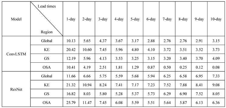
The following quantifies the RMSE difference (denoted as the RMSE reduction percentage) of the forecasted SSTs when using the U-Transformer model compared with the SSTs forecasted using the ConvLSTM and ResNet models (
Table 1), particularly in the regions with active mesoscale eddies. At the 1-day lead time, the U-Transformer model achieves RMSE reductions of 20.42% and 21.32% in the KE region, 12.19% and 16.82% in the GS region, and 10.41% and 25.79% in the OSA region relative to the ConvLSTM and ResNet models, respectively. Globally, the U-Transformer model reduces the RMSEs by 10.13% compared with the ConvLSTM model and by 11.66% compared with the ResNet model. As the lead time increases, the RMSE reduction percentages also decrease. For example, at the 10-day lead time, compared with the ConvLSTM and ResNet models, the RMSE reductions for the U-Transformer model decrease to 3.73% and 9.08% in the KE region, 4.09% and 8.05% in the GS region, and 0.08% and 6.36% in the OSA region, respectively. This comparison demonstrates that the U-Transformer model consistently outperforms the other two models, not only in terms of forecast SSTs globally but also for forecast SSTs in the regions with active mesoscale eddies. This is important when forecasting SSTs induced by mesoscale eddies.
4. Discussion and Conclusions
This study used the U-Transformer model to forecast global short-term SST, and compared its performance with that of the ConvLSTM and ResNet models. The U-Transformer model consistently outperformed the other two models, achieving the lowest RMSEs globally, ranging from 0.2–0.54 °C for 1- to 10-day lead times, with larger ACC of 0.97–0.79. Notably, the RMSEs produced by the U-Transformer model at the 1-day lead time were more than 10% smaller than those of the ConvLSTM and ResNet models.
In regions with active mesoscale eddies, such as the KE, GS, and OSA, the U-Transformer model also produced smaller RMSEs and higher ACC values. It reduced the RMSEs by 20.42% and 21.32% in the KE region, 12.19% and 16.82% in the GS region, and 10.41% and 25.79% in the OSA region, compared with those of the ConvLSTM and ResNet models, respectively. However, the RMSEs in these regions were 40%–130% above those of the global average, reflecting the difficulty in forecasting short-term SSTs in regions with active mesoscale eddies. The richness of mesoscale eddies or swift perturbation processes leads to strong nonlinearity because of their large energy and motion. The RMSE is generally low (<0.2 °C) in the tropical and subtropical oceans, except the eastern equatorial Pacific, where the influence of the TIW results in significantly higher prediction errors (>0.3 °C). In TIW regions, strong shear instability are dominated. It is very obvious mesoscale perturbation process. This underscores the challenges of accurately forecasting SST in regions dominated by strong nonlinear dynamics and complex interactions. Such traits can lead to a more rapid loss of skills related to short-term forecasting of SSTs in such areas.
The good performance demonstrated by the U-Transformer model implies that the use of the self-attention mechanism can recognize pattern connections and nonlinear (eddies having strong nonlinear features) temporal relationships, which can enhance the ability for short-term SST forecasting in the regions with active mesoscale eddies.
These findings of this study emphasize the importance of selecting appropriate DL models for accurate SST forecasting, especially in regions characterized by complex physical processes. Future research should explore strategies intended to improve model performance in relation to forecasting in such challenging regions. Key directions for improving SST forecasting accuracy include incorporating physical constraints into neural networks, integrating physical prior knowledge [
14,
15], and designing more diverse input variables.
Figure 1.
(a) Architecture of the U-Transformer model and (b) two successive Swin Transformer Blocks.
Figure 1.
(a) Architecture of the U-Transformer model and (b) two successive Swin Transformer Blocks.
Figure 2.
Variation of different evaluation metrics with lead time (1- to 10-day) for the three DL models (i.e., the U-Transformer, ConvLSTM, and ResNet models): (a) RMSEs, (b) Bias, (c) ACC during 2020–2022. Metrics were obtained through global weighted averaging.
Figure 2.
Variation of different evaluation metrics with lead time (1- to 10-day) for the three DL models (i.e., the U-Transformer, ConvLSTM, and ResNet models): (a) RMSEs, (b) Bias, (c) ACC during 2020–2022. Metrics were obtained through global weighted averaging.
Figure 3.
Comparison of different model forecasts with observations from TAO/PIRATA/RAMA buoys in different oceans. (a, b) Pacific; (c, d) Atlantic; (e, f) Indian. The a, c, and e represent the distribution and RMSE of spatial points across various oceans, as forecasted 1-day lead time by the U-Transformer. Panels (b), (d), and (f) display the RMSE and ACC of different models at varying lead times, where the solid line represents the RMSE, and the dashed line represents the ACC.
Figure 4.
Spatial distribution of RMSEs for 1-day (a, d, g), 5-day (b, e, h), and 10-day (c, f, i) lead times by the U-Transformer model during 2020–2022 (a–c), by the ConvLSTM model (d–f), and by the ResNet model (g–i). Global average RMSE values are displayed in the upper-right corner of each panel. Dashed boxes indicate the locations of selected regions with active mesoscale eddies: the Kuroshio Extension (30°–40°N, 140°–170°E), Gulf Stream (35°–55°N, 40°–80°W), and the oceans around Southern Africa (35°–45°S, 10°–45°E).
Figure 5.
Global SST from observation and forecasts from three DL models, at 1-day leading (January 1, 2022), 5-days leading (January 5, 2022) starting from January 1, 2022. (a-c) OISST; (d-f) U-Transformer; (g-i) ConvLSTM; (j-l) ResNet. RMSEs and pattern correlation coefficients (R) of forecast SST from models and observations in the upper right corner. The first and second columns display the raw SST values, with thin black contour intervals representing 4℃ isotherms and thick black lines denoting 28℃ isotherms. The third column shows the filtered mesoscale signal obtained by subtracting the low-pass filtered SST (3°x3°) from the raw SST values.
Figure 6.
Comparison of OISST and SST forecasts by three deep learning models in the Kuroshio Extension region from July 14, 2022, to July 20, 2022. The first row represents OISST, while the second, third, and fourth rows show forecasts biases from the U-Transformer, ConvLSTM, and ResNet models.
Figure 6.
Comparison of OISST and SST forecasts by three deep learning models in the Kuroshio Extension region from July 14, 2022, to July 20, 2022. The first row represents OISST, while the second, third, and fourth rows show forecasts biases from the U-Transformer, ConvLSTM, and ResNet models.
Figure 7.
Forecast SST from forecast cases from the U-Transformer, ConvLSTM, and ResNet at the 1-day lead time using the same forecast initial value. These cases are selected according to the 10th percentile (smaller RMSE) of the sorted RMSE values by ascending order for the U-Transformer in three eddy-active regions (Kuroshio Extension, Gulf Stream, and the oceans around Southern Africa). The average RMSE values for each area are displayed in the upper-right corner of each panel. Panels (a-c) correspond to forecasts initialized on December 19, 2021; panels (d-f) forecasts initialized on October 6, 2022; and panels (g-i) forecasts initialized on January 1, 2022.
Figure 8.
Forecast SST from forecast cases from the U-Transformer, ConvLSTM, and ResNet at the 1-day lead time using the same forecast initial value. These cases are selected according to the 90th percentile (larger RMSE) of the sorted RMSE values by ascending order for the U-Transformer in three eddy-active regions (Kuroshio Extension, Gulf Stream, and the oceans around Southern Africa). The average RMSE values for each area are displayed in the upper-right corner of each panel. Panels (a-c) correspond to forecasts on August 30, 2020; panels (d-f) forecasts on June 3, 2020; and panels (g-i) forecasts on February 13, 2021.
Figure 9.
Comparison of RMSEs and ACC values across three regions with active mesoscale eddies for different models at various lead times (a, c, e). Solid lines represent RMSEs and dashed lines represent ACC values. Panels (b, d, f) show the percentage increase in RMSEs within the selected regions (denoted RMSEc) compared with the global average RMSEs (denoted RMSEd), calculated as ((RMSEc − RMSEd)/RMSEd) × 100%.
Table 1.
Percentage reduction in RMSE () of the U-Transformer model (denoted ) compared with the different models (denoted ) across various regions, including the global region and the three regions with active mesoscale eddies: the Kuroshio Extension (KE), Gulf Stream (GS), and oceans around Southern Africa (OSA).