Deep Learning-Based Segmentation for Terrain Classification in Aerial Imagery

1. Introduction

Due to the effective use of agricultural image processing and its high performance, semantic segmentation has gained recognition as a significant research topic and has been employed extensively in numerous agricultural domains in recent years ([1], [2], [3], [4]). Deep learning techniques are important in the agriculture sector and in mapping landcover using remote sensing high spatial resolution (HSR) ([5], [6]). Monitoring land cover is crucial for natural resource management, and these high-resolution photos, known as remote sensing photographs, can be utilized extensively for agricultural and landcover classifications [7]. Several fields of activity, including precision agriculture [8], urban planning [9, 10], environmental protection, land resource management and land classification can take great advantage of remote sensing. The literature on semantic segmentation is extensive and includes a large variety of datasets, of which we give some examples of the most popular. One of these is SpaceNet MVIO, an open-source Multiview Overhead Imagery dataset [11] used for segmentation and object detection tasks. The outcomes are produced in three areas:

1)Expanding object detection and segmentation models to previously unseen

resolutions;

2) Detecting buildings;

3) Confirm whether resolution adjustments for segmentation and object detection models had an impact and do research on them and their consequences. One dataset that can be used for semantic segmentation of agricultural patterns is Agriculture-vision, which is composed of extensive aerial field photos [12]. This dataset has been analyzed using popular semantic segmentation models, specifically DeeplabV3+.

Other works include one that uses a better Unet model to apply semantic segmentation to rice lodging, Xin Zhao et al. [13], and another that uses SOMs and a Deeplab CNN to segment remote sensing data in agriculture [3]. Multilayer perceptrons (MLPs) and RF classifiers are used in work concerning the classification of crop types and land cover [4]. Semantic segmentation has been applied to UAV-acquired pictures [14] by comparing various approaches, including DeeplabV3+, EfficientNet, FPN, and AGN, with the author's approach, AgriSegNet, a model whose backbone characteristics are extracted from the DeepLabV3+ mode.

Other works see the application of U-Net to segmentation in the agriculture of wheat [15] and an application of an adapted version of VGG-16, a deep neural network semantic segmentation of mixed crops [16]. Many works are present in literature about the segmentation of crop, weed, and background of which we give two examples: an encoder-decoder network trained to recognize weed, crop, and background [17], and a deep learning model of U-Net trained to segment weed and crop [18]. Javiera Castillo-Navarro is credited with work on MiniFrance [19], a dataset designed for semisupervised learning. In the relative work two networks perform semantic segmentation: BerundaNet and W-Net.

Monitoring and assessing land cover and land use are crucial agricultural practices [20]. Remote sensing data is helpful in order to monitor landscape and agricultural activities and enables the study of the rate of urbanization, deforestation, and agricultural intensity ([8], [9], [10], [21], [12]). Most of these investigations use multispectral satellite imagery, which can be most expensive when obtained at high resolution. Although a study of land mapping can be conducted through transfer learning of existing networks, a comparative analysis of how this transfer learning functions more or less depending on the neural network chosen has not yet been conducted, in order to accurately determine its utility for the agriculture sector.

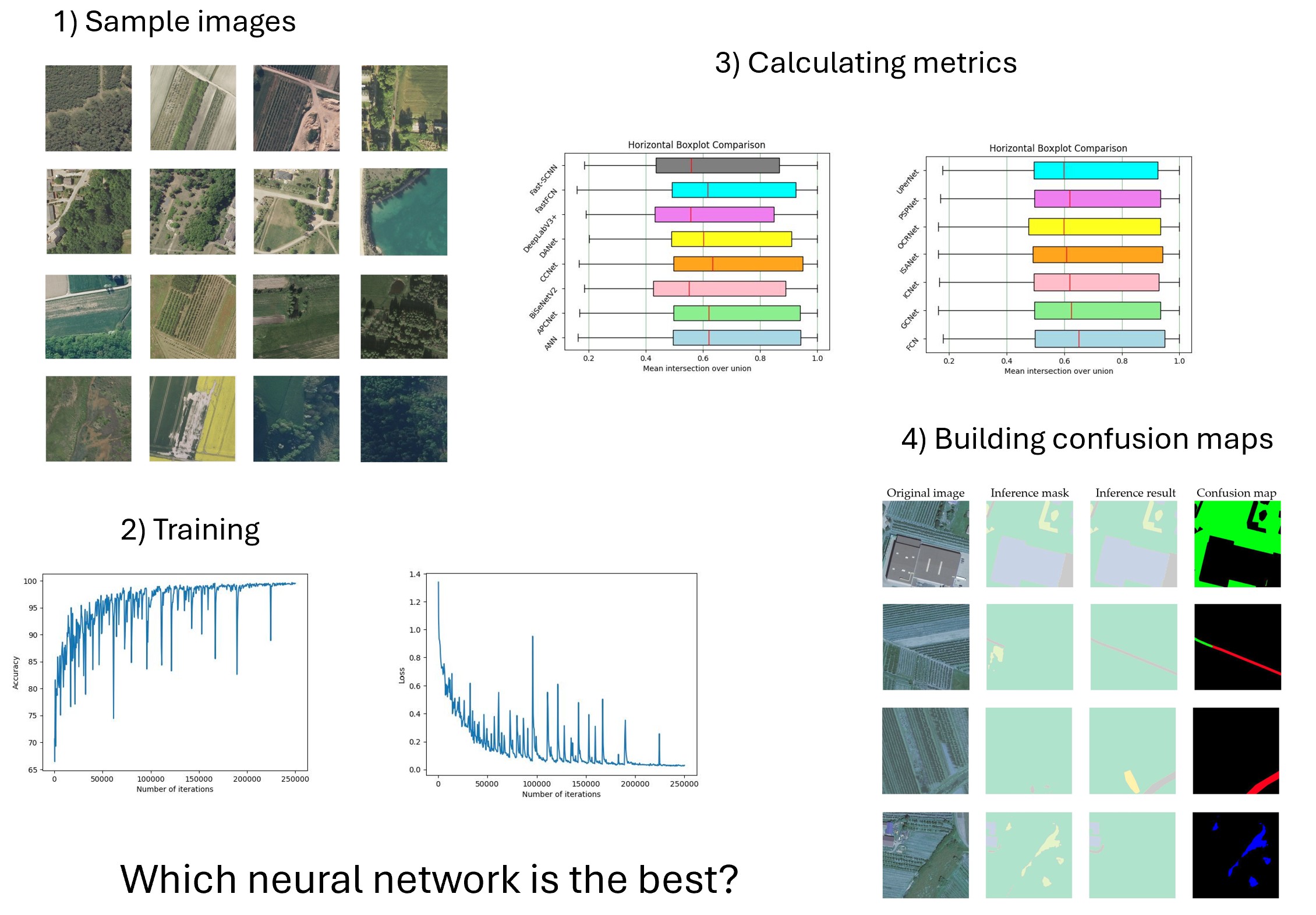
In this research, we aim to identify the best models for agriculture image segmentation by analyzing outliers and evaluating the quality of existing semantic segmentation models. This work was carried out according to the following steps:

• first of all, we select according to their performances fifteen neural networks, at the state of the art, created using the MMSegmentation toolbox [22] for Python to apply semantic segmentation, and metrics like accuracy, intersection over union (IoU) and recall are assessed;

• second, we use statistical tools to analyze the results and identify the networks that perform best;

• third, confusion maps are created to determine the type and quality of eventual misclassifications, and a comparison of those networks is then carried out by examining the quantity and quality of errors committed. The images in which vision gives origin to a mistake are the so-called outliers. Finally, we provide a summary of the best networks with a low number of relevant network mistakes.

The rest of the paper is divided into three chapters. Chapter 2 contains a brief description of the dataset, LandCover.ai, the segmentation methods, and performance evaluation metrics. Chapter 3 presents the experimental results and discussion. Chapter 4 concludes our paper, opening the road to future insights of the research.

2. Materials and Methods

2.1. Data Preparation

First, we arrange data preparation, so that data are processed and converted from their original state to one more suitable for the subsequent analysis [23]. The LandCover.ai dataset consists of 8 images with a resolution of 50 cm (about 4200 x 4700 pixels) and 33 photographs with a resolution of 25 cm (approximately 9000 x 9500 pixels). As Adrian Boguszewski [7] did, since most networks have an input range between 200 and 1024 pixels, we split 41 originals and respective masks into 512 x 512-pixel smaller ones. There are 10674 photos and 10674 masks in total, excluding smaller ones. 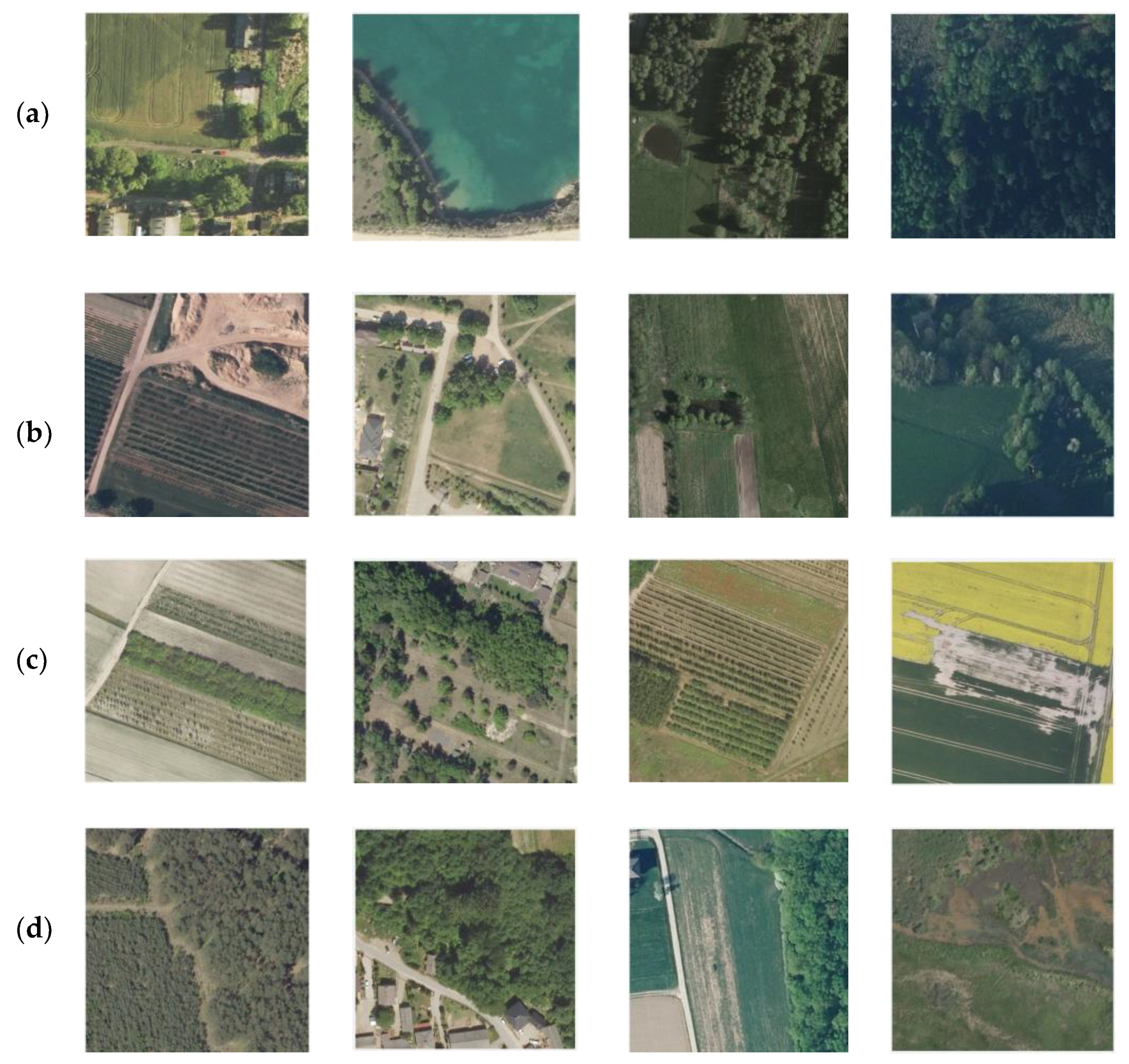Figure 1 shows a selection of photos in the dataset after a split of originals.

2.2. Semantic Segmentation Neural Networks

In this work, semantic segmentation of the LandCover.ai dataset is performed using Python and 15 networks trained via the MMSegmentation tools within the Python framework. This framework is offered by MMSegmentation, an open toolbox suitable for the consistent use and assessment of semantic segmentation techniques. Most well-known semantic segmentation techniques and datasets have excellent fine-tunings available in MMSegmentation. Accuracy, intersection over union, and recall are the metrics computed as mean metrics with respect to each class in semantic segmentation tasks. Now, the description of the used networks in this work is as follows.

2.2.1. Asymmetrical Non-Local Neural Network for Semantic Segmentation (ANN) [24]

In the Asymmetric Non-local Neural Network, the semantic segmentation spatial feature extraction can be enhanced by implying non-local operations that encapsulate long-range dependencies, hence enhancing segmentation accuracy by paying attention to both local and global context information of an image. [23]. The Asymmetric Pyramid Non-local Block (APNB) and Asymmetric Fusion Non-local Block (AFNB) are integrated into a pyramid sampling module to drastically decrease computation time and memory use and at the same time grant good results. Different levels of features are combined, which improves performance.

2.2.2. APCNet [25]

Point cloud processing focuses on optimizing deep semantic segmentation networks. It incorporates context features through attention mechanisms, improving performance, by applying APCNet (Attention Pyramid Context Network).Multiple well-drawn Adaptive Context Modules (ACMs) are located within multiscale contextual representations produced by APCNet. A context vector is computed when the local affinity coefficient associated with each sub-region is assessed by each ACM.

2.2.3. BiSeNetV2 [26]

BiSeNetV2 is a real-time semantic segmentation model that enhances its feature extraction and segmentation through both the spatial and context path. Its architecture permits holding little features usually overlooked in speeding up elaboration thanks to its in-core features Branch and Semantic Branch. This will increase the elaboration accuracy significantly.

2.2.4. CCNet [27]

Image segmentation is enhanced by CCNET (Criss-Cross Network) enhances image segmentation by using cluster-based representations and dense cross-level connections. Consequently, it can be assigned an accurate semantic label to each pixel.

Each pixel in the image is provided with a semantic class label. However, because of the rigid geometric structures of this network, is difficult to find an answer to issues in some FCN applications where a quicker and more accurate understanding of images is needed. Criss Cross Network can extract more comprehensive and contextual information from every pixel.

2.2.5. DANet [28]

The scope of focusing on relevant features of images and improving them can be obtained by employing the Dual Attention Network (DAN) which integrates both spatial and channel-wise attention mechanisms.

With the help of a Dual Attention Network for Scene Segmentation is possible to determine the positions of the various items in the image, and detailed dependencies can be represented in both spatial and channel dimensions thanks to a position attention module and a channel attention model.

2.2.6. DeepLabV3+ [29]

Deep neural networks for semantic segmentation tasks can use Spatial pyramid pooling module, in order to encode multiscale informations by intercepting the incoming features, or can use an encode decoder structure to catch thin object boundaries and to compose all the spatial details. DeepLabV3+ combines the advantages of both methods, by adding to the previous DeepLabV3 a decoding module to obtain better defined boundaries of the objects in the scene.

2.2.7. FastFCN [30]

FastFCN is a semantic segmentation model that relates the efficacy of fully convolutional networks (FCNs) with a quick, excellent output. It manages a unique lightweight encoder-decoder architecture that decreases computational complexity while preserving performance. FastFCN pioneers a dilated convolution procedure to extend the receptive subject, advancing contextual insight. The model also improves segmentation by using a more efficient feature fusion strategy, increasing fine-grained details. This makes FastFCN appropriate for real-time segmentation tasks, uniquely on resource-constrained machines.

2.2.8. Fast-SCNN [31]

A Fast Semantic Segmentation Convolutional Neural Network (CNN) is designed to proficiently match pixel-wise class labels to images while diminishing computational complexity. Commonly techniques are employed like dilated convolutions, reduced network depth, and lightweight architectures for faster processing.A fast segmentation network for real-time scene understanding is the focus of R. R. K. Poudel’s work. This network is required when images need to be analyzed rapidly in or-der to provide a prompt reaction or develop a rapid or binding action based on the envi-ronmental situation. Furthermore, the work shows that further applications to auxiliary tasks do not require additional pre-training once the model has been suitably trained.

2.2.9. FCN [32]

Fully Convolutional Network (FCN) is a deep learning architecture constructed for semantic image segmentation. Unlike traditional CNNs that output fixed-size feature maps, FCNs substitute totally connected layers with convolutional layers, granting the network to construct pixel-wise expectations. FCNs use an encoder-decoder construction, where the encoder describes high-level features and the decoder upsamples to create segmentation maps. Skip connections are often used to preserve fine-grained spatial information from earlier layers. FCNs are widely assumed for tasks expecting dense pixel-level classification, such as scene understanding and medical image analysis.

2.2.10. GCNet [33]

Segmentation accuracy can be improved by incorporating global context through a self-attention mechanism, as CGNet (Global Context Network) is deputed to perform, capturing long-range dependencies in the input image. GCNet is able to capture the long-term dependencies and connections between images or scenes separated by significant periods of time with less computation and the same accuracy by simplifying the network to take into account that many queries are the same in different regions of a picture and by concentrating the analysis only in the parts of the images that shows changes.

2.2.11. ICNet [34]

Image Cascade Network (ICNet) is a semantic segmentation model designed for efficient real-time performance by increasingly improving estimates through a multi-resolution method. It uses a cascade construct to handle images at distinctive resolutions, balancing accuracy and speed.

The Image Cascade Network (ICNet) is a real time semantic segmentation system that produces a fast elaboration of the images, in order to provide real time scene parsing in all the situations where immediate and deep understanding of the scene is required and speedy is a critical factor for action. For istance, it is the case of automatic driving and of all robotic interactions. Moreover, thanks to a new framework which saves operations in multiple resolutions, and to a powerfull fusion unit, ICNet grants an optimal union of accuracy and speed.

2.2.12. ISANet [35]

An Image Spatial Attention Network (ISANet) enhances the focal point at salient regions of an image via learning of spatial attention maps. It enhances feature representation for object detection and image classification. ISANet puts a high value on improvement in suitability of the self-attention mechanism for semantic segmentation.The two following attention modules evaluate the two sparse affinity matrices that make up its structure. Processing high-resolution feature maps decreases computing and memory complexity.

2.2.13. OCRNet [36]

The Object Contextual Representations Network (OCR-Net) improves object segmentation by uniting object context knowledge through adaptive contextual learning, by integrating object context information through adaptive contextual learning. Capturing detailed object boundaries and long-range dependencies in the way to obtain a higher accuracy. The OC-Rnet operates in three main steps: first, a deep network determines a rough soft segmentation; second, the description for each object region is estimated by compiling the descriptions with respect to pixels in the corresponding object region. Third, OCR is used to enrich each pixel’s description.

2.2.14. PSPNet [37]

Pyramid Scene Parsing Network (PSPNet) is a deep learning model constructed for semantic segmentation where a pyramid pooling module is used to obtain multi-scale context information from an image. Segmentation accuracy is enhanced by contemplating both local and global contextual information at several spatial scales.

The target of scene parsing is that of attributing each pixel in the image a category label, the function for which PSPNet is designed. Pyramid scene parsing network has the property to merge proper global features. The pixel-level feature is extended to the especially created global pyramid pooling one, additionally to conventional enlarged FCN [3, 40] for pixel prediction. The local and global traces together make the ultimate forecast more consistent.

2.2.15. UperNet [38]

With Unified Perceptual Parsing for Scene Understanding, multiple scene understanding are fused into a single model. UperNet simultaneously handles semantic segmentation, depth estimation, and object recognition for the complete study.

In order to simulate the complexity of human vision as closely as possible, Unified Perceptual Parsing is a multitasking framework that can identify a large number of objects features, and situations in an image at the same time. As a result, it can catalog and process a large amount of information, construct segments, and elaborate a large number of concepts.

2.3. Training

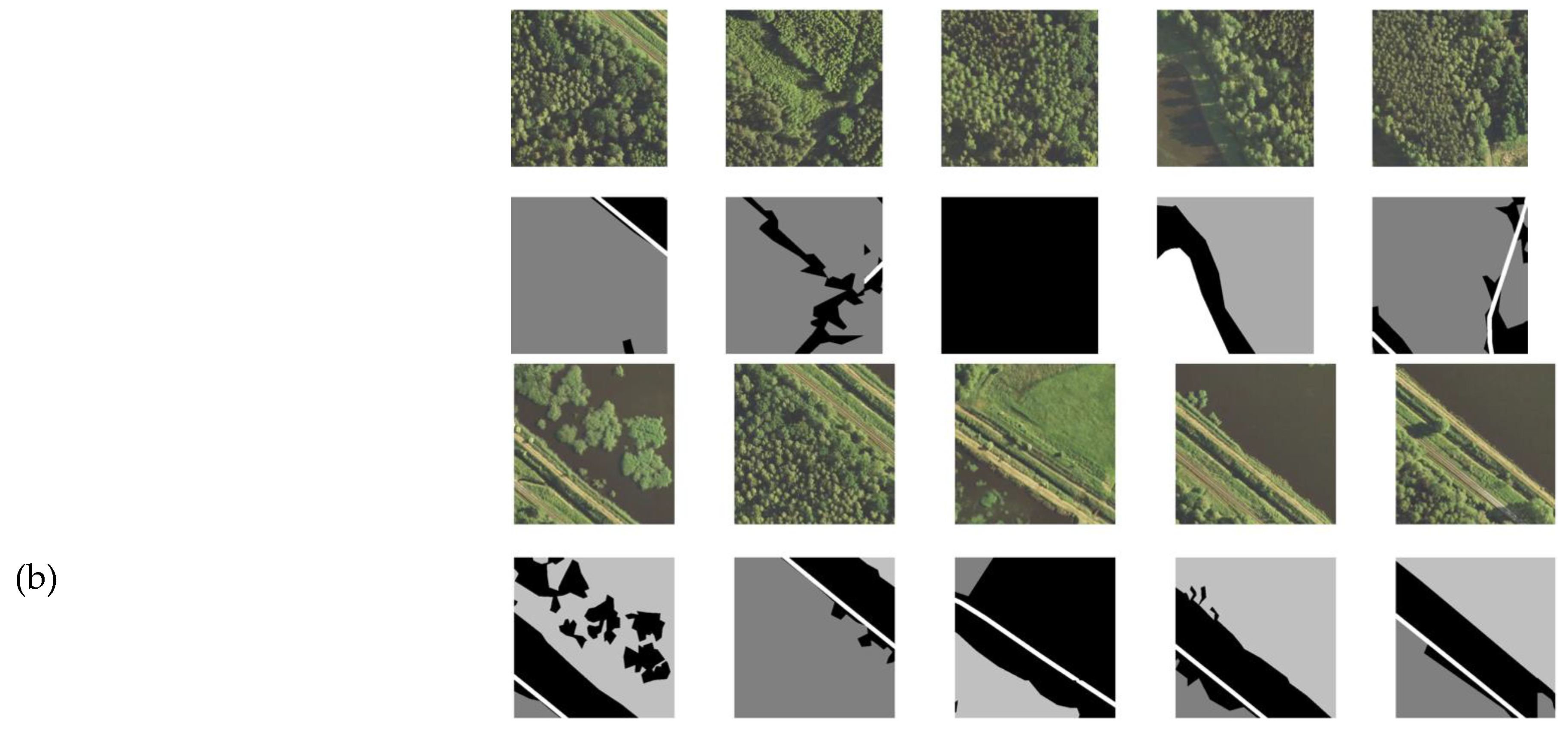
After having attended to data preparation, which consists of dividing the images into smaller ones, the dataset must be split into train and test sets. We select 500 photos for the test set and undersample the other 10174 images because the original dataset is unbal-anced ([39], [40], [41]). In our case, only a small percentage of pixels are labeled as belonging to the less represented class of water, while the most represented pixels refer to the woodland class. We add undersampling to the training set by choosing images with more balanced classes because we think that appropriate undersampling can be helpful. 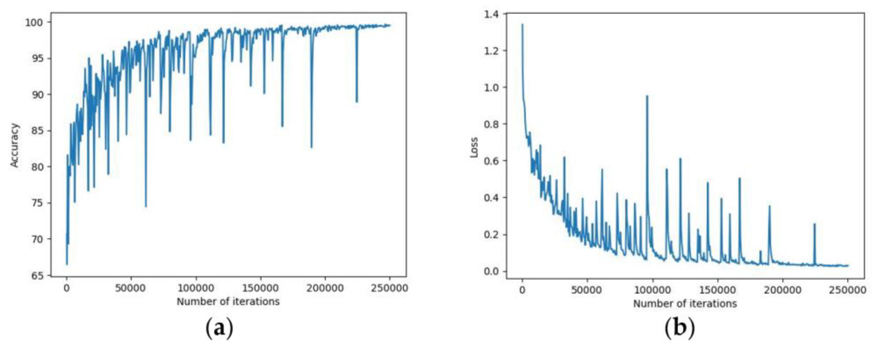The number of pixels for each of the classes is summed for each of the greyscale masks.The Individual Images and masks are then taken when four out of five classes have a minimum of one thousand pixels affixed.A selection of our photos and respective masks both with and without undersampling is presented in Figure 2. We create a training set of 250000 iterations for every network over the entire dataset, saving at each 50000 iteration and returning accuracy and loss values every 2500 iterations.

Other parameters of the training are the learning rate of 0.01, with a momentum of 0.9, type=’SGD’, and a weight decay of 0.0005, optimization function SGD, and batch size equal to 1.As a criterion of evaluating the performance we chose the accuracy and loss on the training and validation sets as a performance metric. Figure 3 shows the accuracy and loss trend for the Network ANN during the training phase. We utilize accuracy, intersection over union, and recall in their mean values and on all five classes to evaluate the model once it has been trained.

2.4. Study of the Outliers

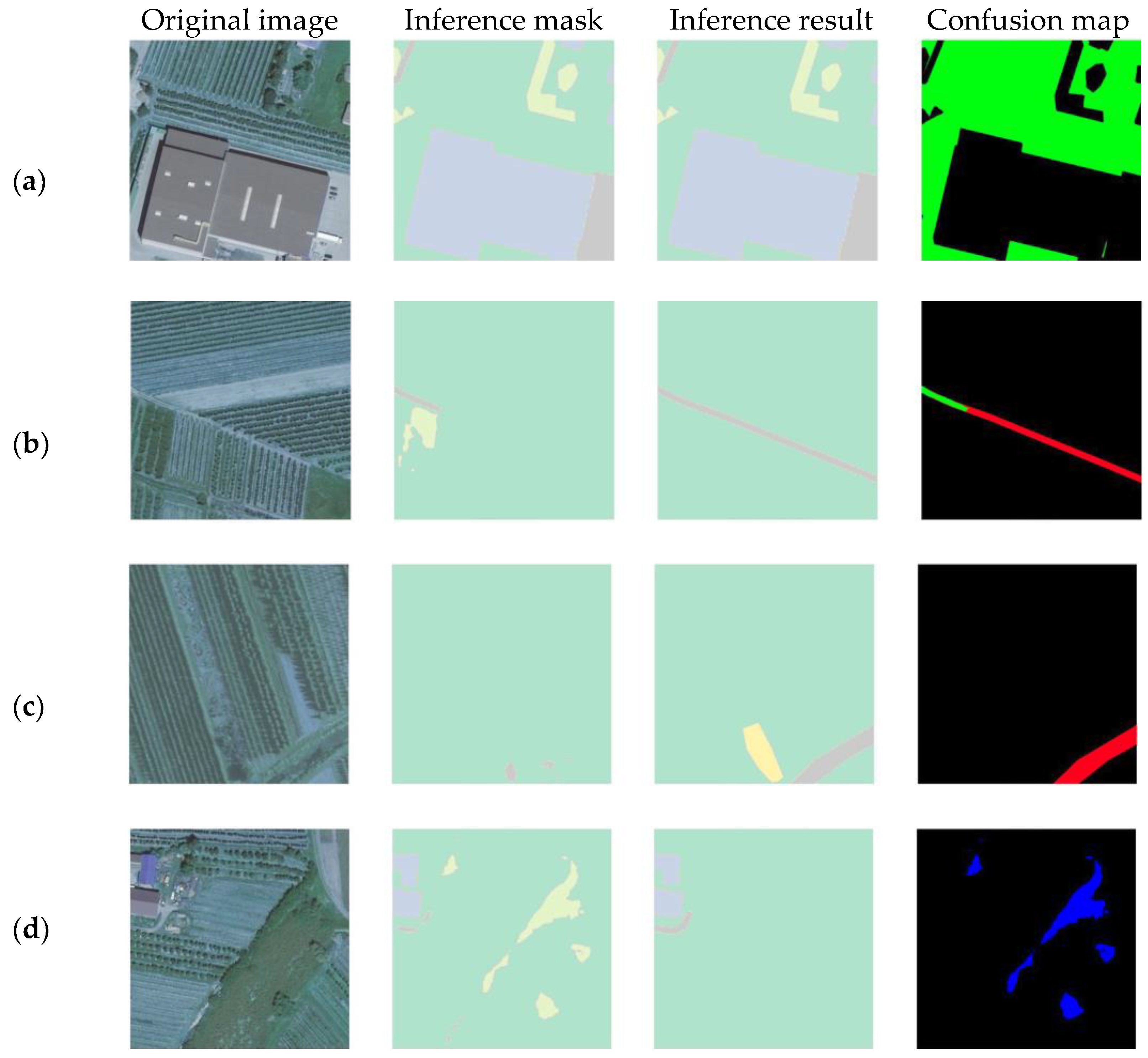
Now, have a detailed look at the outliers after figuring out the segmentation task metrics. We calculate outliers for each class and analyze them. First, we analyze outliers with res-pect to intersection over union because it is the most important. Intersection over union is a physical definition and assesses the level of overlying between the ground truth region and the prediction region; because Accuracy depends on binary cross-entropy. According to the following rule, we first produce a “confusion map” for each class. This is a fourth image colored in three distinct ways according to the different pixel categories: 1. Where the prediction of the network is similar to the ground truth, pixels are green as shown in Figure 4. These are called true positives (subfigure (a) and (b));

2. the red pixels in subfigure (b) and (c) are called “false negatives”, as the network fails to forecast the relevant class, in opposite to the ground truth (fig 4); 3. The blue pixels in subfigure (d) are known as false positives in subfigure (d); in this case, the network correctly predicts the right class but the prediction is not present in the ground truth picture pixels (fig. 4). Now, we surely can assess that while the ground truth frequently makes mistakes, the neural network frequently performs right. As an example, in subfigure d the neural network correctly distinguishes road, while the ground truth doesn’t, making a mistake.

Above, we classified the various cases of misclassifications, now we are going on to a through analysis of the outliers.

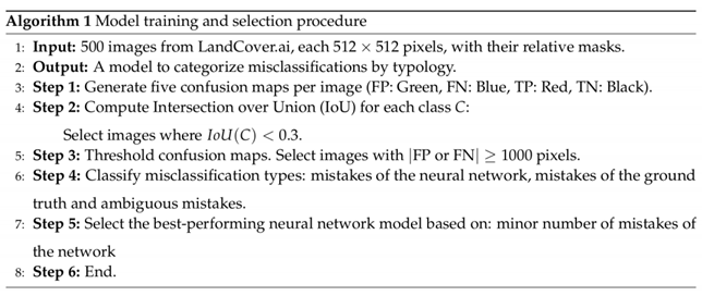
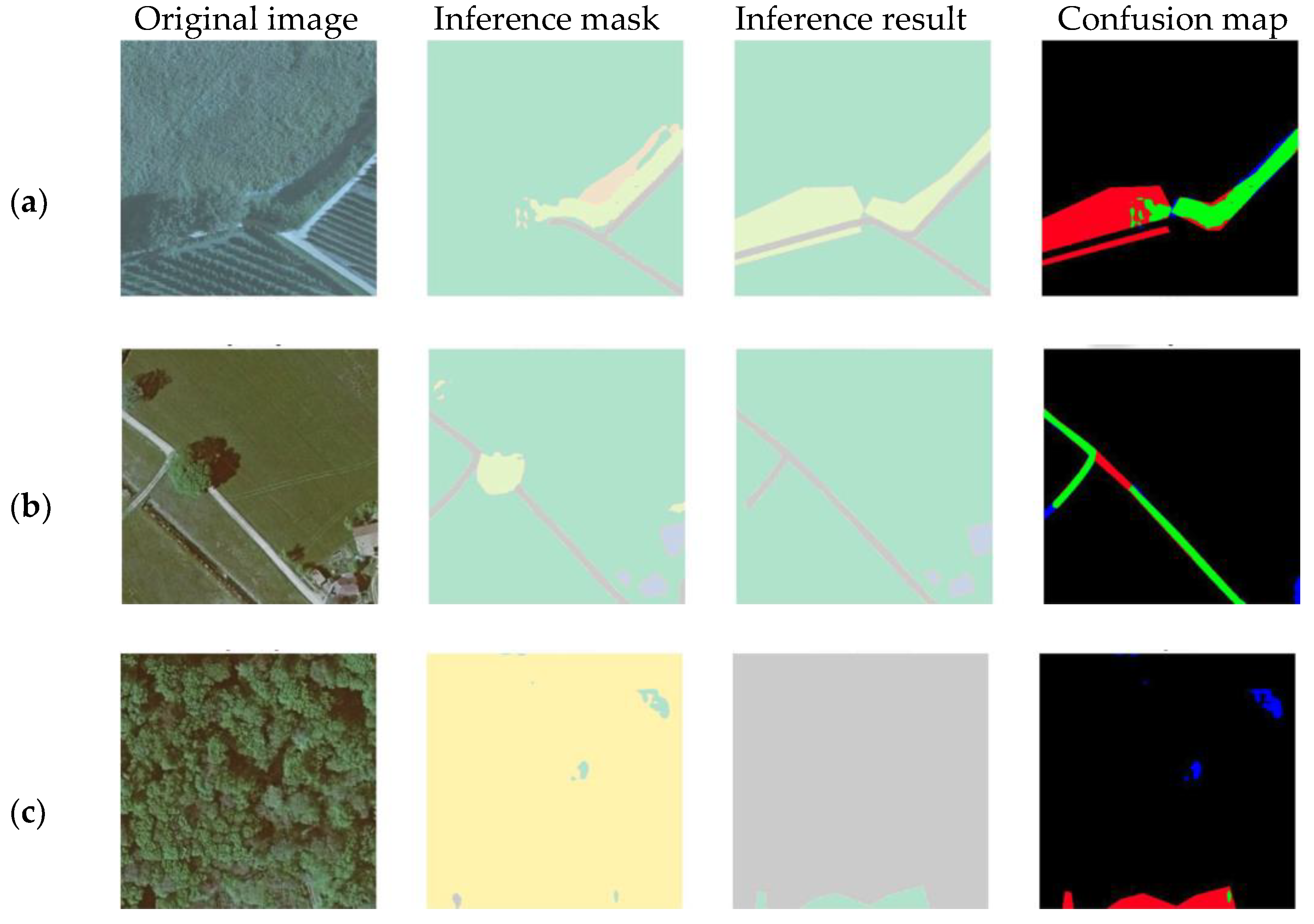
In this step, to examine each of the 500 test set photos of the outliers, we rely on the three-pixel categories. As explained above, we create five confusion maps for each original image in the dataset, coloring the pixels according to the classes represented in them. We then selected the confusion maps where the intersection over the union of the associated class is less than 0.3. Subsequently, we defined threshold confusion maps in which at least 1000 pixels are either red or blue, that is where the image was correctly predicted. The next step was to classify the three kinds of misclassifications for each selected image, defined as follows, according to the different colors of pixels (fig. 5):

• mistakes of the network; is the case in which the neural network makes a mistake while the ground truth is correct. For example, in subfigure a the image has been traced with respect to the woodland, but the neural network doesn’t recognize as woodland a part of the image that should be classified as woodland while the ground truth does;

• mistakes of the ground truth; in this case, the ground truth occurs in an error while the neural network classifies correctly the contents of the image. Subfigure b presents the case of an image in which the neural network recognizes a tree correctly, while the ground truth doesn’t;

• ambiguous mistakes, cases not falling under either of the first two. These are the cases in which the original image is confused. In these cases, we cannot impute the hypothetical errors either at the ground truth or at the neural network. For instance, subfigure c represents an image traced with respect to background, in which the neural network classifies as background that part of the image corresponding to shadows, in blue, while the ground truth doesn’t. Whether it is right to classify shadows as background is an ambiguous case. Also in the red pixels there is an ambiguity between background and woodland, since it is not clear where the area covered by trees finishes.

The proposed method is the pseudo-code 1 for the algorithm of model training and selection procedure.

3.1. Experimental Setup

The performance of fifteen distinct neural networks is demonstrated by the use of semantic segmentation techniques, evaluated in the first phase on performance metrics like recall, accuracy and intersection over union. As the second step of this experiment, we individuate the outliers by creating confusion maps of the 500 test set photos according to the five distinct classes. Finally, it has been possible to determine the frequency of various mistakes types regarding the liable actors such as network, ground truth, and ambiguous mistakes for each of the fifteen networks throughout the entire test set.

3.2. Results of Semantic Segmentation

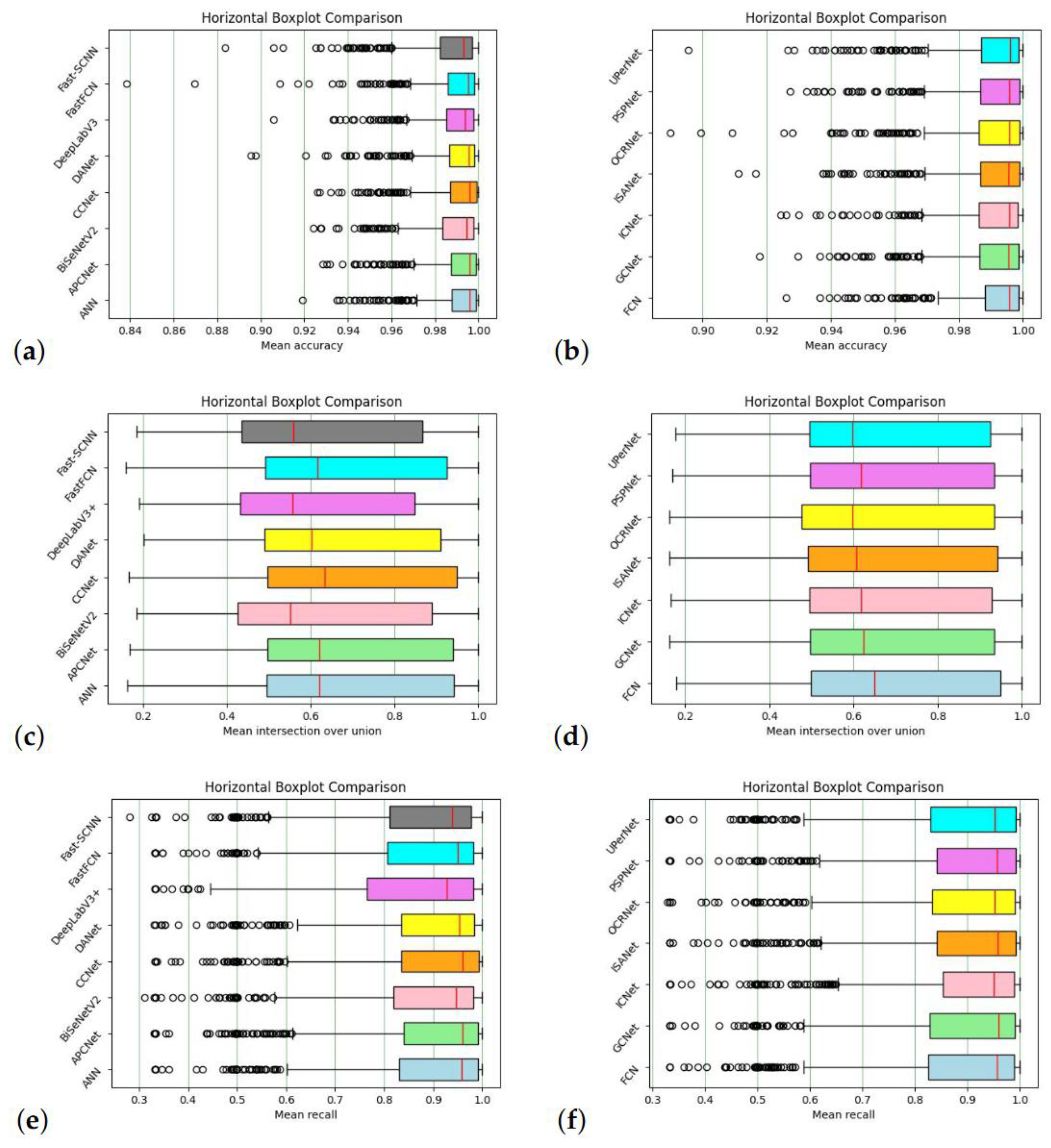
Accuracy, IoU and recall are the parameters used to assess the model in relation to the semantic segmentation problem. In this work, they are computed on all five classes and in their mean values for each of the fifteen networks chosen and are reported as boxplots in Figure 6, with the following mean values for all networks: intersection over union is above 60%, accuracy in its mean value is above 98%, and recall is above 85%, as shown in boxplots (fig. 6). The values in subfigures a and b are clustered around the mean value, the variance accuracy is low.

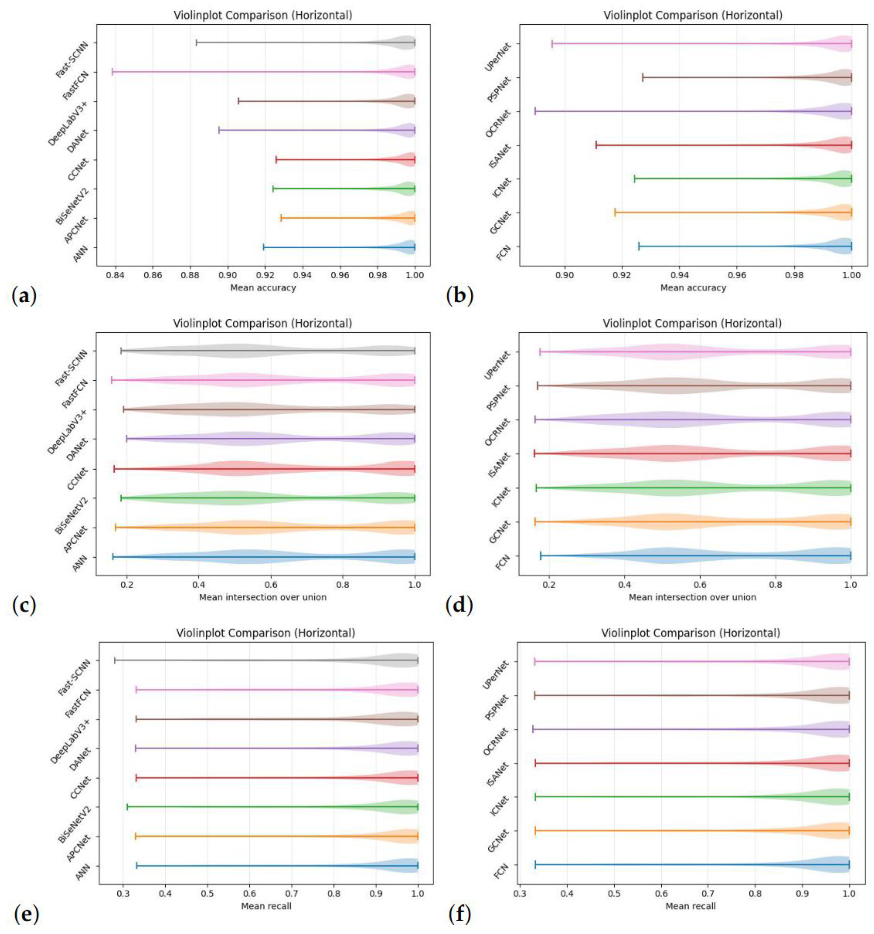
The IoU variance is higher in subfigures (c) and (d). In terms of dimensions, the variance in subfigures e and f is between the first two. The violin plots for the fifteen networks that reflect mean accuracy, mean intersection over union, and mean recall are shown in Fig. 7. This picture portrays a scenario similar to violin plots and one that we assess in our case: subfigure a and b have a smaller variance in accuracy, subfigure (c) and (d) have a larger variance in IoU, and subfigure e and f have a recall variance positioned between the first two. Our models achieve an accuracy of 99.06%, with a 71.5% of intersection over union (IoU) and 88.43% of recall. Table 1 shows the accuracy results obtained for each class along with the mean values. The results of intersection over union for all classes, together with their mean values, are presented in Table 2.

Table 3 presents the recall results for each class along with the mean values.

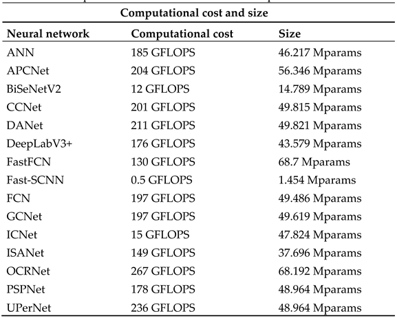
In Table 4 the computational costs and sizes of the networks are reported.Moreover, we must recognize that where there are buildings and woodland neural net-works work better, while they perform worse in the presence of water and roads.

Always about performances of the different neural networks we can assess that FCN performs best regarding accuracy, followed by APCNet. The best network in terms of intersection over union is CCNet, which is followed by FCN; in terms of recall, the best network is ICNet, which is followed by PSPNet.

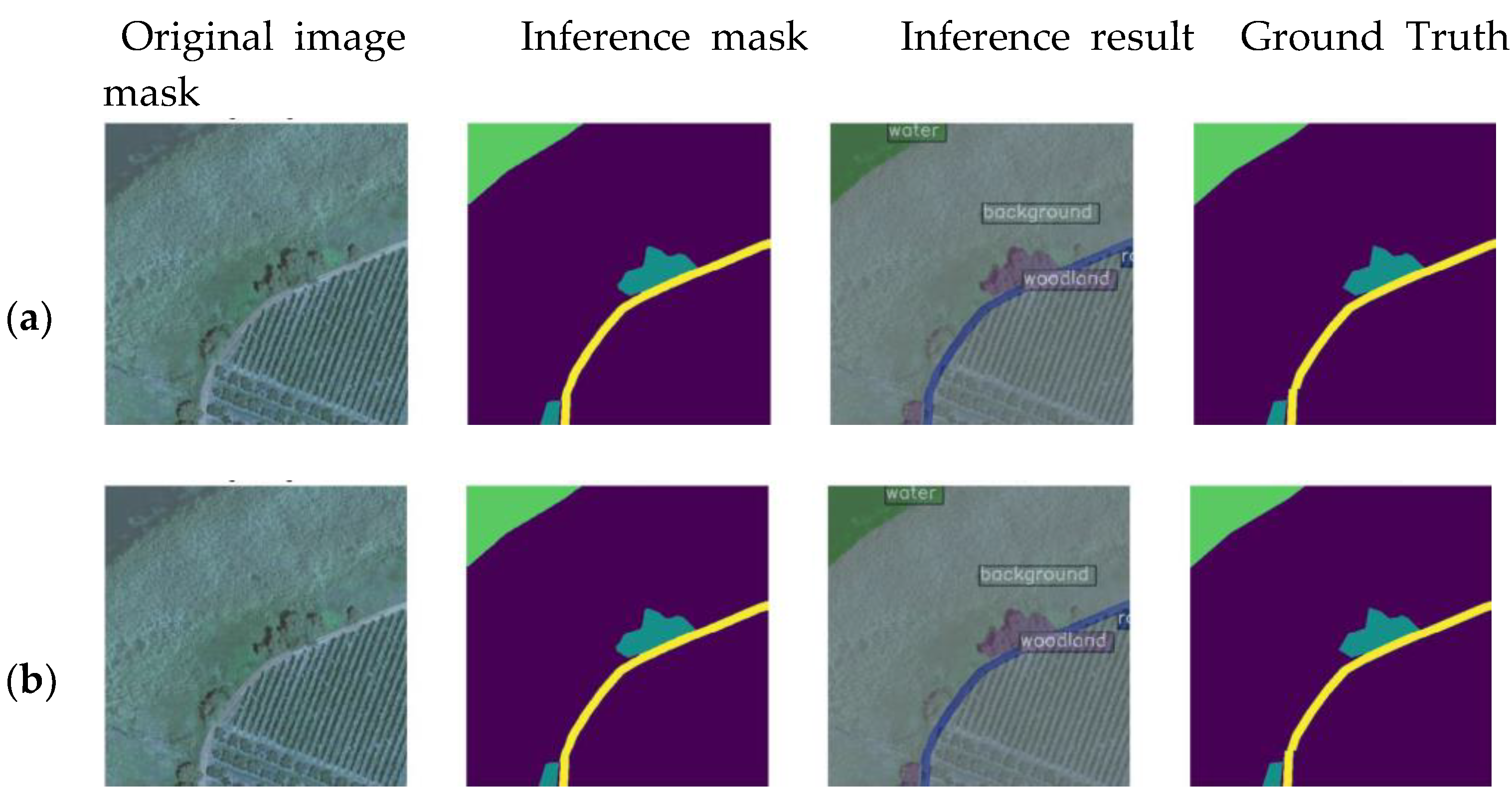
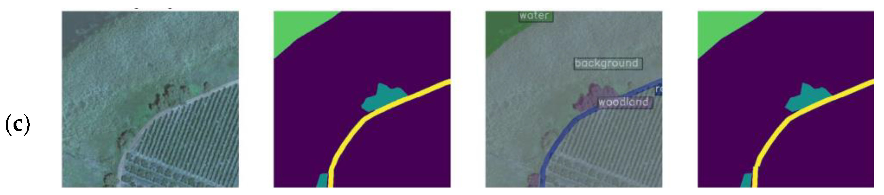
Using the feature of the MMSegmentation library, we make inferences. First we have a model, then an image, and then an inference is made. Figure 8 is a demonstration inference with three neural networks over an image taken in a landcover.ai dataset with both an original and an inference mask. Given the buildings and trees, we can determine that the road is well-known. Regarding the network mistakes, PSPNet is the neural network that performs best followed by FCN and UPerNet, the two other networks that exhibit good performance in terms of the overall amount of mistakes and mistakes in the network.

3.3. Results of the Study of the Outliers

In Table 5 the results of this study of outliers are reported. We investigate the outliers aiming at classifying the misclassifications. We indicate the neural networks that perform best as those networks in correspondence of which fewer mistakes are due to the neural networks. The network that performs best is PSPNet with 21 mistakes of the network, followed by FCN with 26 mistakes and UPerNet with 28 mistakes, always of the neural network, while as regard the total number of mistakes the neural networks which perform best are FCN, PSPNet and ANN. We can say that as regard per class results there is not a network which outperforms the others, there is no need of ANOVA test to understand it: for example we have that PSPNet is the network which performs best in terms of total number mistakes related to the class background, which is not the best network as regard the total number of mistakes related to the class woodland and roads. The best network as regard the total number of mistakes related to the class woodland are ANN and ISANet, as regard the total number of mistakes related to the class roads the best network is FCN, as regard the total number of mistake related to class water is PSPNet, as regards the total number of mistakes related to class buildings the best networks are CCNet, ICNet, ISANet and PSPNet. We choose as a metric on which to conduct our analysis the intersection over union, since it is a measure of how much the two surfaces (the ground truth region and

Table 1. Accuracy across 15 networks.

						Accuracy
Neural network	Background		Buildings		Woodland		Water	Roads	Mean accuracy
ANN	0.9770		0.9990(1)		0.9825		0.9974	0.9957	0.9903
APCNet	0.9775(2)		0.9990(1)		0.9830(2)		0.9978(1)	0.9956	0.9906(2)
BiSeNetV2	0.9732		0.9984		0.9800		0.9969	0.9952	0.9887
CCNet	0.9770		0.9990(1)		0.9825		0.9976(2)	0.9956	0.9904
DANet	0.9752		0.9989(2)		0.9821		0.9963	0.9956	0.9896
DeepLabV3	0.9742		0.9987		0.9811		0.9974	0.9949	0.9896
FastFCN	0.9739		0.9987		0.9814		0.9960	0.9953	0.9891
Fast-SCNN	0.9686		0.9981		0.9770		0.9958	0.9942	0.9867
FCN	0.9779(1)		0.9990(1)		0.9835(1)		0.9977	0.9960(1)	0.9908(1)
GCNet	0.9764		0.9990(1)		0.9824		0.9981	0.9951	0.9902
ICNet	0.9769		0.9989(2)		0.9828		0.9973	0.9958	0.9904
ISANet	0.9759		0.9990(1)		0.9817		0.9972	0.9957	0.9899
OCRNet	0.9745		0.9990(1)		0.9815		0.9960	0.9955	0.9893
PSPNet	0.9765		0.9989(2)		0.9820		0.9978(1)	0.9956	0.9902
UPerNet	0.9758		0.9989(2)		0.9821		0.9965	0.9959(2)	0.9899

Maximum value in correspondence of each label and in correspondence of the mean value. Second value in correspondence of each label and in correspondence of the mean value.

Table 1. Accuracy across 15 networks.

						Accuracy
Neural network	Background		Buildings		Woodland		Water	Roads	Mean accuracy
ANN	0.9770		0.9990(1)		0.9825		0.9974	0.9957	0.9903
APCNet	0.9775(2)		0.9990(1)		0.9830(2)		0.9978(1)	0.9956	0.9906(2)
BiSeNetV2	0.9732		0.9984		0.9800		0.9969	0.9952	0.9887
CCNet	0.9770		0.9990(1)		0.9825		0.9976(2)	0.9956	0.9904
DANet	0.9752		0.9989(2)		0.9821		0.9963	0.9956	0.9896
DeepLabV3	0.9742		0.9987		0.9811		0.9974	0.9949	0.9896
FastFCN	0.9739		0.9987		0.9814		0.9960	0.9953	0.9891
Fast-SCNN	0.9686		0.9981		0.9770		0.9958	0.9942	0.9867
FCN	0.9779(1)		0.9990(1)		0.9835(1)		0.9977	0.9960(1)	0.9908(1)
GCNet	0.9764		0.9990(1)		0.9824		0.9981	0.9951	0.9902
ICNet	0.9769		0.9989(2)		0.9828		0.9973	0.9958	0.9904
ISANet	0.9759		0.9990(1)		0.9817		0.9972	0.9957	0.9899
OCRNet	0.9745		0.9990(1)		0.9815		0.9960	0.9955	0.9893
PSPNet	0.9765		0.9989(2)		0.9820		0.9978(1)	0.9956	0.9902
UPerNet	0.9758		0.9989(2)		0.9821		0.9965	0.9959(2)	0.9899

Maximum value in correspondence of each label and in correspondence of the mean value. Second value in correspondence of each label and in correspondence of the mean value.

Table 2. Intersection over union across 15 networks.

Intersection over union
Neural network	Background	Buildings	Woodland	Water	Roads	Mean IoU
ANN	0.8391(1)	0.6702	0.6341	0.3382	0.5254	0.6689
APCNet	0.8438	0.6746	0.6276	0.3741	0.5139	0.6711
BiSeNetV2	0.8267	0.5311	0.5804	0.2932	0.4566	0.6172
CCNet	0.8389(2)	0.6636	0.6474(2)	0.4118	0.5196	0.7150(1)
DANet	0.8374	0.6502	0.6289	0.3385	0.4699	0.6496
DeepLabV3	0.8338	0.5642	0.5805	0.3136	0.4017	0.6132
FastFCN	0.8325	0.6194	0.6210	0.3843	0.4822	0.6567
FCN	0.8402	0.7086(2)	0.6526(1)	0.4467(2)	0.5456(1)	0.6967(2)
Fast-SCNN	0.8224	0.5165	0.5815	0.2861	0.4338	0.6082
GCNet	0.8367	0.6594	0.6232	0.4931(1)	0.5060	0.6782
ICNet	0.8417	0.7085(1)	0.6305	0.3429	0.4967	0.6654
ISANet	0.8370	0.6660	0.6241	0.3380	0.5145	0.6550
OCRNet	0.8355	0.6259	0.6312	0.3307	0.5034	0.6551
PSPNet	0.8391(1)	0.6168	0.6214	0.4278	0.5116	0.6673
UPerNet	0.8321	0.6604	0.6265	0.3428	0.5299(2)	0.6608

Maximum value in correspondence of each label and in correspondence of the mean value. Second value in correspondence of each label and in correspondence of the mean value.

Table 2. Intersection over union across 15 networks.

Intersection over union
Neural network	Background	Buildings	Woodland	Water	Roads	Mean IoU
ANN	0.8391(1)	0.6702	0.6341	0.3382	0.5254	0.6689
APCNet	0.8438	0.6746	0.6276	0.3741	0.5139	0.6711
BiSeNetV2	0.8267	0.5311	0.5804	0.2932	0.4566	0.6172
CCNet	0.8389(2)	0.6636	0.6474(2)	0.4118	0.5196	0.7150(1)
DANet	0.8374	0.6502	0.6289	0.3385	0.4699	0.6496
DeepLabV3	0.8338	0.5642	0.5805	0.3136	0.4017	0.6132
FastFCN	0.8325	0.6194	0.6210	0.3843	0.4822	0.6567
FCN	0.8402	0.7086(2)	0.6526(1)	0.4467(2)	0.5456(1)	0.6967(2)
Fast-SCNN	0.8224	0.5165	0.5815	0.2861	0.4338	0.6082
GCNet	0.8367	0.6594	0.6232	0.4931(1)	0.5060	0.6782
ICNet	0.8417	0.7085(1)	0.6305	0.3429	0.4967	0.6654
ISANet	0.8370	0.6660	0.6241	0.3380	0.5145	0.6550
OCRNet	0.8355	0.6259	0.6312	0.3307	0.5034	0.6551
PSPNet	0.8391(1)	0.6168	0.6214	0.4278	0.5116	0.6673
UPerNet	0.8321	0.6604	0.6265	0.3428	0.5299(2)	0.6608

Maximum value in correspondence of each label and in correspondence of the mean value. Second value in correspondence of each label and in correspondence of the mean value.

Table 3. Recall across 15 networks.

Recall
Neural network	Background	Buildings	Woodland	Water	Roads	Mean IoU
ANN	0.9375	0.8414	0.8482	0.8278(1)	0.7802	0.8815
APCNet	0.9389	0.8405	0.8506	0.8105	0.7798	0.8823
BiSeNetV2	0.9333	0.8148	0.8400	0.8025	0.7472	0.8704
CCNet	0.9338	0.8483(2)	0.8575	0.8141	0.7807	0.8828
DANet	0.9403	0.8276	0.8502	0.7998	0.7594	0.8776
DeepLabV3	0.9443(2)	0.7832	0.8001	0.8187	0.6769	0.8540
FastFCN	0.9356	0.8245	0.8297	0.7573	0.7447	0.8656
Fast-SCNN	0.9264	0.7986	0.8334	0.7759	0.7359	0.8628
FCN	0.9501(1)	0.8202	0.8336	0.7902	0.7615	0.8772
GCNet	0.9382	0.8398	0.8523	0.7850	0.7771	0.8807
ICNet	0.9417	0.8452	0.8544	0.8100	0.7788	0.8843(1)
ISANet	0.9356	0.8378	0.8570	0.8198(2)	0.7872(1)	0.8836
OCRNet	0.9340	0.8403	0.8628(1)	0.8195	0.7847(2)	0.8834
PSPNet	0.9364	0.8498(1)	0.8609(2)	0.8148	0.7808	0.8842(2)
UPerNet	0.9371	0.8475	0.8517	0.8129	0.7684	0.8806

Maximum value in correspondence of each label and in correspondence of the mean value. Second value in correspondence of each label and in correspondence of the mean value.

Table 3. Recall across 15 networks.

Recall
Neural network	Background	Buildings	Woodland	Water	Roads	Mean IoU
ANN	0.9375	0.8414	0.8482	0.8278(1)	0.7802	0.8815
APCNet	0.9389	0.8405	0.8506	0.8105	0.7798	0.8823
BiSeNetV2	0.9333	0.8148	0.8400	0.8025	0.7472	0.8704
CCNet	0.9338	0.8483(2)	0.8575	0.8141	0.7807	0.8828
DANet	0.9403	0.8276	0.8502	0.7998	0.7594	0.8776
DeepLabV3	0.9443(2)	0.7832	0.8001	0.8187	0.6769	0.8540
FastFCN	0.9356	0.8245	0.8297	0.7573	0.7447	0.8656
Fast-SCNN	0.9264	0.7986	0.8334	0.7759	0.7359	0.8628
FCN	0.9501(1)	0.8202	0.8336	0.7902	0.7615	0.8772
GCNet	0.9382	0.8398	0.8523	0.7850	0.7771	0.8807
ICNet	0.9417	0.8452	0.8544	0.8100	0.7788	0.8843(1)
ISANet	0.9356	0.8378	0.8570	0.8198(2)	0.7872(1)	0.8836
OCRNet	0.9340	0.8403	0.8628(1)	0.8195	0.7847(2)	0.8834
PSPNet	0.9364	0.8498(1)	0.8609(2)	0.8148	0.7808	0.8842(2)
UPerNet	0.9371	0.8475	0.8517	0.8129	0.7684	0.8806

Maximum value in correspondence of each label and in correspondence of the mean value. Second value in correspondence of each label and in correspondence of the mean value.

Table 5. Study of the outliers.

		ANN	APCNet	BiSeNetV2	CCnet	DANet	DeepLabV3+	FastFCN	Fast_SCNN	FCN	GCNet	ICNet	ISANet	OCRNet	PSPNet	UPerNet
Mistakes of the network
background		9	8	11	7	3	10	11	11	11	15	9	12	15	5	6
buildings		1	3	1	0	1	0	2	2	0	2	0	0	4	0	1
woodland		19	16	12	8	7	11	14	14	7	17	7	9	13	4	7
water		9	26	9	3	8	0	2	2	1	13	4	3	33	0	7
road		8	23	16	13	10	20	19	19	7	25	7	9	22	12	7
Total mistakes of network		46	76	49	31	29	41	48	48	26	72	27	33	87	21	28
Mistakes of the ground truth
background		17	7	3	13	7	11	14	14	9	15	9	14	17	16	11
buildings		0	4	0	0	1	0	2	2	0	3	0	0	3	0	1
woodland		10	53	28	22	17	23	27	27	17	55	16	20	60	15	16
water		0	2	0	0	0	0	0	0	0	1	0	0	0	0	0
road		14	22	16	11	13	10	13	13	10	27	13	12	23	11	8
Total mistakes of the groundtruth		41	88	47	46	38	44	56	56	36	101	38	46	103	42	36
Ambiguous mistakes
background		29	35	44	30	47	41	53	53	33	24	33	35	32	16	39
buildings		0	5	2	0	0	2	4	4	1	0	0	0	1	0	0
woodland		43	4	65	45	59	58	68	68	36	6	52	43	3	66	66
water		2	1	7	4	7	6	3	3	3	3	6	5	2	0	4
road		13	15	19	19	20	20	32	32	10	17	21	18	15	20	9
Total ambiguous mistakes		87	60	137	98	133	127	160	160	83	50	112	101	53	102	118
Total
background		55	50	58	50	57	62	78	78	53	54	51	61	64	37	56
buildings		1	12	3	0	2	2	8	8	1	5	0	0	8	0	2
woodland		72	73	105	75	83	92	109	109	60	78	75	72	76	85	89
water		11	29	16	7	15	6	5	5	4	17	10	8	35	0	11
road		35	60	51	43	43	50	64	64	27	69	41	39	60	43	24
Total		174	224	233	175	200	212	264	264	145	223	177	180	243	165	182

the prediction region) are overlapping.

Table 5. Study of the outliers.

		ANN	APCNet	BiSeNetV2	CCnet	DANet	DeepLabV3+	FastFCN	Fast_SCNN	FCN	GCNet	ICNet	ISANet	OCRNet	PSPNet	UPerNet
Mistakes of the network
background		9	8	11	7	3	10	11	11	11	15	9	12	15	5	6
buildings		1	3	1	0	1	0	2	2	0	2	0	0	4	0	1
woodland		19	16	12	8	7	11	14	14	7	17	7	9	13	4	7
water		9	26	9	3	8	0	2	2	1	13	4	3	33	0	7
road		8	23	16	13	10	20	19	19	7	25	7	9	22	12	7
Total mistakes of network		46	76	49	31	29	41	48	48	26	72	27	33	87	21	28
Mistakes of the ground truth
background		17	7	3	13	7	11	14	14	9	15	9	14	17	16	11
buildings		0	4	0	0	1	0	2	2	0	3	0	0	3	0	1
woodland		10	53	28	22	17	23	27	27	17	55	16	20	60	15	16
water		0	2	0	0	0	0	0	0	0	1	0	0	0	0	0
road		14	22	16	11	13	10	13	13	10	27	13	12	23	11	8
Total mistakes of the groundtruth		41	88	47	46	38	44	56	56	36	101	38	46	103	42	36
Ambiguous mistakes
background		29	35	44	30	47	41	53	53	33	24	33	35	32	16	39
buildings		0	5	2	0	0	2	4	4	1	0	0	0	1	0	0
woodland		43	4	65	45	59	58	68	68	36	6	52	43	3	66	66
water		2	1	7	4	7	6	3	3	3	3	6	5	2	0	4
road		13	15	19	19	20	20	32	32	10	17	21	18	15	20	9
Total ambiguous mistakes		87	60	137	98	133	127	160	160	83	50	112	101	53	102	118
Total
background		55	50	58	50	57	62	78	78	53	54	51	61	64	37	56
buildings		1	12	3	0	2	2	8	8	1	5	0	0	8	0	2
woodland		72	73	105	75	83	92	109	109	60	78	75	72	76	85	89
water		11	29	16	7	15	6	5	5	4	17	10	8	35	0	11
road		35	60	51	43	43	50	64	64	27	69	41	39	60	43	24
Total		174	224	233	175	200	212	264	264	145	223	177	180	243	165	182

the prediction region) are overlapping.

So not always the discrepancy between neural network prediction and ground truth is due to a mistake of the neural network, but sometimes it is a human mistake and other

times it is an ambiguous case, so the actual predictive power of neural networks is superior. In our research we investigate all the cases, distinguishing the best networks and values of accuracy, intersection over union and recall. These metrics are calculated as a function of true positives, false positives, true negatives and false negatives.

3. Discussion

The CNN architecture of our models is conformable enough to adjust to the different data elements and attributes of agricultural images since semantic methods of segmentation and their applications in agriculture have evolved rapidly in recent years. As previously said, the inaccurate classification is not always due to the network; in many cases it is due to the ground truth. Then, there are cases in which also the human eye can occur in an error, because of confused images, these are called ambiguous mistakes. The best models thus depend on the situation where the network gives the minor number of mistakes rather than just the best values of accuracy, recall, and intersection over union.

In this study, using the deep learning MMSegmentation toolbox fifteen neural networks are trained to generate semantic segmentation algorithms. For each of the five classes chosen three metrics—accuracy, intersection over union, and recall—are determined as mean quantities. Segmentation tasks are developed using the MSegmentation Toolbox. Images used in this work are described as background, building, woodland, water, and road.

To choose the best model out of all networks under consideration, we report accuracy, intersection over union, and recall values in terms of violin plots and boxplots. With aforementioned settings, we have best models for inference in precision agriculture. For five classes, we report aforementioned values (recall, accuracy, and intersection over union) as well.The best networks, in our conclusion for outliers in terms of intersection over union, evaluating performances in respect of network mistakes, are PSPNet, FCN, and UperNet. In any case we put on evidence that a combination of neural networks can give better results in specific cases.The images considered in such an outlier analysis are simply called confusion maps, and labelled true positives, false positives, true negatives, and false negatives with respect to a target class.As indicated in section 2.4. intersection over union defines the level of overlapping of the reading of the surfaces as for the ground truth and the prediction region. The images are selected when the intersection over union is smaller than 0.3. These cases are called outliers. The examination of outliers is carried out with regard to the intersection over union across all five classes, as indicated in section 2.4. Subsequently, a study is carried out with the objective of classifying the test set's photos according to the typology of misclassifications, distinguishing between mistakes of the network, mistakes of the ground truth, and ambiguous mistakes.

5. Conclusions

The judging of the increasing application of deep CNN in agriculture and in its study in general is the prerogative of this work, after having explored the LandCover.ai dataset and the semantic segmentation. Our goal then is to understand the model that is best performing for studying precision agriculture and its characteristics. We considered that precision agriculture has unique "image patterns" which are well different from those in which most segmentation networks were developed (medicine, automotive,...), hence the effectiveness of transfer learning among these fields may differ as well. So we conduct the study of those patterns in agriculture through semantic segmentation algorithms by choosing fifteen neural networks and the study of the outliers aiming at finding those models which perform best not just taking into account metrics such as accuracy, intersection over union and recall, but the kind of misclassifications encountered.

For the future we are planning to apply these development methodologies to new datasets, for example a dataset formed by the Copernicus images, to get information about agricultural areas. In fact there is not yet generalizability in passing from local (i.e. LandCover.ai dataset) to global (i.e. world images) level, therefore from aerial images to satellite images. The techniques used for the development of this project can also be used on some datasets of images detected by drones by selecting the best-performing system on a case-by-case basis, depending on the type of detection, with the understanding that for some applications in the area of agriculture both detection systems can be used.

References

- Rong, C.; Fu, W. A Comprehensive Review of Land Use and Land Cover Change Based on Knowledge Graph and Bibliometric Analyses. Land 2023, 12, 1573Talukdar, S.; Singha, P.; Mahato, S.; Pal, S.; Liou, Y.A.; Rahman, A. Land-use land-cover classification by machine learning classifiers for satellite observations—A review. Remote Sens. 2023, 12, 1135.
- Luo, Z.W.; Yuan, Y.; Gou, R.; Li, X. Semantic segmentation of agricultural images. A survey. Information Processing in Agriculture 2023. [Google Scholar] [CrossRef]
- Jadhav, J.K.; Singh, R. Automatic semantic segmentation and classification of remote sensing data for agriculture. Mathematical Models in Engineering 2018, 4, 112–137. [Google Scholar] [CrossRef]
- Kussul, N.; Lavreniuk, M.; Skakun, S.; Shelestov, A. Deep learning classification of land cover and crop types using remote sensing data. IEEE Geoscience and Remote Sensing Letters 2017, 14, 778–782. [Google Scholar] [CrossRef]
- Dhanya, V.; Subeesh, A.; Kushwaha, N.; Vishwakarma, D.K.; Kumar, T.N.; Ritika, G.; Singh, A. Deep learning based computer vision approaches for smart agricultural applications. Artificial Intelligence in Agriculture 2022, 6, 211–229. [Google Scholar] [CrossRef]
- Attri, I.; Awasthi, L.K.; Sharma, T.P.; Rathee, P. A review of deep learning techniques used in agriculture. Ecological Informatics 2023, p. 102217.
- Boguszewski, A.; Batorski, D.; Ziemba-Jankowska, N.; Dziedzic, T.; Zambrzycka, A. LandCover. ai: Dataset for automatic mapping of buildings, woodlands, water and roads from aerial imagery. Proceedings of theence on Computer Vision and Pattern Recognition, 2021.
- Maggiori, E.; Tarabalka, Y.; Charpiat, G.; Alliez, P. Convolutional neural networks for large-scalere mote-sensing image classification. IEEE Transactions on geoscience and remote sensing 2016, 55, 645–657 1102. [Google Scholar] [CrossRef]
- Pauleit, S.; Duhme, F. Assessing the environmental performance of land cover types for urban planning. Landscape and urban planning 2000, 52, 1–20. [Google Scholar] [CrossRef]
- Zhou, W.; Huang, G.; Cadenasso, M.L. Does spatial configuration matter? Understanding the effects of land cover pattern on land surface temperature in urban landscapes. Landscape and urban planning 2011, 102, 54–63. [Google Scholar]
- Weir, N.; Lindenbaum, D.; Bastidas, A.; Etten, A.V.; McPherson, S.; Shermeyer, J.; Kumar, V.; Tang, H. Spacenet mvoi: A multi-view overhead imagery dataset. Proceedings of the ieee/cvf international conference on computer vision, 2019, pp.992-1001.
- Chiu, M.T.; Xu, X.; Wei, Y.; Huang, Z.; Schwing, A.G.; Brunner, R.; Khachatrian, H.; Karapetyan, H.; Dozier, I.; Rose, G. ; others. Agriculture-vision: A large aerial image database for agricultural pattern analysis. Proceedings of the IEEE/CVF Conference on Computer Vision and Pattern Recognition, 2020, pp. 2828.2838.
- Zhao, X.; Yuan, Y.; Song, M.; Ding, Y.; Lin, F.; Liang, D.; Zhang, D. Use of unmanned aerial vehicle imagery and deep learning unet to extract rice lodging. Sensors 2019, 19, 3859. [Google Scholar] [CrossRef] [PubMed]
- Anand, T.; Sinha, S.; Mandal, M.; Chamola, V.; Yu, F.R. AgriSegNet: Deep aerial semantic segmentation framework for IoT-assisted precision agriculture. IEEE Sensors Journal 2021, 21, 17581–17590. [Google Scholar] [CrossRef]
- Liu, G.; Bai, L.; Zhao, M.; Zang, H.; Zheng, G. Segmentation of wheat farmland with improved U-Net on drone images. Journal of applied remote sensing 2022, 16, 034511–034511. [Google Scholar] [CrossRef]
- Mortensen, A.K.; Dyrmann, M.; Karstoft, H.; Jørgensen, R.N.; Gislum, R. Semantic segmentation of mixed crops using deep convolutional neural network. 2016.
- Wang, A.; Xu, Y.; Wei, X.; Cui, B. Semantic segmentation of crop and weed using an encoder-decoder network and image enhancement method under uncontrolled outdoor illumination. Ieee Access 2020, 8, 81724–81734. [Google Scholar] [CrossRef]
- Sahin, H.M.; Miftahushudur, T.; Grieve, B.; Yin, H. Segmentation of weeds and crops using multispectral imaging imaging and CFR- enhanced U-Net. Computers and Electronics in Agriculture 2023.
- Castillo-Navarro, J.; Le Saux, B.; Boulch, A.; Audebert, N.; Lefèvre, S. Semi-Supervised Semantic Segmentation in Earth Observation: The MiniFrance suite, dataset analysis and multi-task network study. Machine Learning 2022, 111, 3125–3160. [Google Scholar] [CrossRef]
- Chiu, M.T.; Xu, X.; Wei, Y.; Huang, Z.; Schwing, A.G.; Brunner, R.; Khachatrian, H.; Karapetyan, H.; Dozier, I.; Rose, G. ; others. Agriculture-vision: A large aerial image database for agricultural pattern analysis. Proceedings of the IEEE/CVF Conference on Computer Vision and Pattern Recognition, 2020, pp. 2828-2838.
- Md Jelas, I. Deforestation detection using deep learning-based semantic segmentation techniques: a systematic review. Frontiers in Forests and Global Change 2024, 7, 1300060. [Google Scholar] [CrossRef]
- Xu, J., Chen, K., Lin, D.: MMSegmenation. Available online: https://github.com/openmmlab/mmsegmentation.
- Fernandes, A.A.; Koehler, M.; Konstantinou, N.; Pankin, P.; Paton, N.W.; Sakellariou, R. Data preparation: A technological perspective and review. SN Computer Science 2023, 4, 425. [Google Scholar] [CrossRef]
- Zhu, Z.; Xu, M.; Bai, S.; Huang, T.; Bai, X. Asymmetric non-local neural networks for semantic segmentation. Proceedings of the IEEE/CVF international conference on computer vision, 2019, pp. 593–602.
- He, J.; Deng, Z.; Zhou, L.; Wang, Y.; Qiao, Y. Adaptive pyramid context network for semantic segmentation. Proceedings of the IEEE/CVF conference on computer vision and pattern recognition, 2019, pp. 7519–7528.
- Yu, C.; Gao, C.; Wang, J.; Yu, G.; Shen, C.; Sang, N. Bisenet v2: Bilateral network with guided aggregation for real-time semantic segmentation. International journal of computer vision 2021, 129, 3051–3068. [Google Scholar] [CrossRef]
- Huang, Z.; Wang, X.; Huang, L.; Huang, C.; Wei, Y.; Liu, W. Ccnet: Criss-cross attention for semantic segmentation. Proceedings of the IEEE/CVF international conference on computer vision, 2019, pp. 603-612.
- Fu, J.; Liu, J.; Tian, H.; Li, Y.; Bao, Y.; Fang, Z.; Lu, H. Dual attention network for scene segmentation. Proceedings of the IEEE/CVF conference on computer vision and pattern recognition, 2019, pp. 3146–3154.
- Chen, L.C.; Zhu, Y.; Papandreou, G.; Schroff, F.; Adam, H. Encoder-decoder with atrous separable convolution for semantic image segmentation. Proceedings of the European conference on computer vision (ECCV), 2018, pp. 801–818.
- Wu, H.; Zhang, J.; Huang, K.; Liang, K.; Yu, Y. Fastfcn: Rethinking dilated convolution in the backbone for semantic segmentation. arXiv:1903.11816 2019.
- Poudel, R.P.; Liwicki, S.; Cipolla, R. Fast-scnn: Fast semantic segmentation network. arXiv:1902.04502 2019.
- Long, J.; Shelhamer, E.; Darrell, T. Fully convolutional networks for semantic segmentation. Proceedings of the IEEE conference on computer vision and pattern recognition, 2015, pp. 3431–3440.
- Liu, J.; Zhou, W.; Cui, Y.; Yu, L.; Luo, T. GCNet: Grid-like context-aware network for RGB-thermal semantic segmentation. Neurocomputing 2022, 506, 60–67. [Google Scholar] [CrossRef]
- Zhao, H.; Qi, X.; Shen, X.; Shi, J.; Jia, J. Icnet for real-time semantic segmentation on high-resolution images. Proceedings of the European conference on computer vision (ECCV), 2018, pp. 405–420.
- L., Yuan Y., Guo J., Zang C., Chen X., Wang J. Interlaced Sparse Self-Attention for Semantic Segmentation. arXiv:1907.12273 2019.
- Yuan, Y.; Chen, X.; Wang, J. Object-contextual representations for semantic segmentation. Computer Vision–ECCV 2020: 16th European Conference, Glasgow, UK, August 23–28, 2020, Proceedings, Part VI 16. Springer, 2020, pp. 173–190.
- Zhao, H.; Shi, J.; Qi, X.; Wang, X.; Jia, J. Pyramid scene parsing network. Proceedings of the IEEE conference on computer vision and pattern recognition, 2017, pp. 2881–2890.
- Wang, R.; Jiang, H.; Li, Y. UPerNet with ConvNeXt for Semantic Segmentation. 2023 IEEE 3rd International Conference on Electronic Technology, Communication and Information (ICETCI). IEEE, 2023, pp. 764–769.
- Kotsiantis, S.; Kanellopoulos, D.; Pintelas, P.; others. Handling imbalanced datasets: A review. GESTS international transactions on computer science and engineering 2006, 30, 25–36.
- Werner de Vargas, V.; Schneider Aranda, J.A.; dos Santos Costa, R.; da Silva Pereira, P.R.; Victória Barbosa, J.L. Imbalanced data preprocessing techniques for machine learning: a systematic mapping study. Knowledge and Information Systems 2023, 65, 31–57. [Google Scholar] [CrossRef] [PubMed]
- Johnson, J.M.; Khoshgoftaar, T.M. Survey on deep learning with class imbalance. Journal of big data 2019, 6, 1–54. [Google Scholar] [CrossRef]