Submitted:
09 March 2025
Posted:
11 March 2025
You are already at the latest version
Abstract
Earthquakes (EQs) are the most unpredictable and damaging natural disasters. Over the last hundred years the scientific community has been engaged in an intense endeavor to attain a confident and secure method of seismic activity forecasting. So far, despite the efforts, no fully validated method for predicting EQs has been established.
However, research of the last thirty years has documented a substantial number of seismic precursor phenomena, the correct evaluation and application of which may pave the way for the development of a reliable EQ prediction method in the near future. The majority of the recent documented seismic precursors belong to the modern and fast developing field of electro-seismology, while a smaller subset remains within the more traditional domain of classical seismology- geophysics.
This article aims to compile, classify, and assess the most well-documented precursors while also proposing a preliminary framework for their more effective application.
Keywords:
Electro-seismology
; seismicity precursors
; prediction/forecasting
1. Introduction
Seismicity prediction is meaningful only when three fundamental parameters are precisely known: WHERE, WHEN and HOW STRONG a forthcoming EQ (hereafter EQ) will be. For clarity reasons, it is useful to distinguish between “prediction” and “forecasting”. “Forecasting” refers to probabilities and percentages regarding the location, magnitude and possible timing of an EQ over weeks, months or years. This kind of information may increase our knowledge about the mechanisms of seismicity but they contain very little practical value for civil protection. In contrast, “prediction” specifies the exact time, location, and magnitude of impending EQs within very narrow confidence limits. Several attempts have been made to achieve precise EQ predictions, but with limited success. Research methods in EQ prediction can be broadly classified into two major categories: The first category contains Precursor-Based Methods they focus on identifying signals that precede an EQ while the second category contains Pattern-Based Methods which examine geophysical trends that may indicate an impending EQ.
Most seismic research is directed toward identifying precursors, as they are considered more suitable for short-term predictions, whereas geophysical trend analysis is more useful for long-term forecasting ranging from one year to a century.
After decades of research, numerous seismic precursors have been identified, which may contribute to an integrated prediction method. These precursors can be categorized into two broad groups:
The first group contains precursors based on geological phenomena of the ground/underground related to classical seismology / geology, such as volcanic activity, collision of tectonic plates, monitoring of known seismic faults, statistical analysis of past seismic events, changes in lithospheric physical properties, 'trend'-based methods, etc.
In the second group belong precursors of electromagnetic signals detected in the atmosphere spanning from the ground to the base of the ionosphere and beyond.
Over the past thirty years, seismicity research has expanded beyond traditional seismology/ geology and has been constituted a subject of the broader area of physics, especially atmospheric/ionospheric electromagnetism. Pioneering studies have introduced new pathways for seismic research, particularly in defining novel precursors [1,2,3,4].
Hayakawa [5] provided a comprehensive review of EQ precursor studies in Japan, noting that extensive investigation projects started to run after the devastating Kobe EQ (6,9/7,2M in 1995 . This foundation stone has contributed to the emergence of electro-seismology as a specialized and distinct field of study. Preliminary references on geoeletric currents possibly related to EQ precursors were already referred since the beginning of 70s [6,7,8,9,10,11,12,13,14].
However, the first documented case of electromagnetic signals linked to seismic activity is credited to George Moore [15],who detected a substantial magnetic disturbance (100γ) one hour and six minutes before the powerful March, 1964 EQ in Alaska. That pioneering signal was recorded by a magnetometer installed in the city of Kodiak, 30 Km far from the seismic fault and survived by chance after the virtual destruction of the city. One year later, Leonard, and Barnes [16] and Davis, and Baker, [17] described for the first time ionospheric disturbances caused by that EQ in Alaska.
The so called “Good Friday EQ” also known as the «Great Alaska EQ», occurred at 5:36 p.m. local time on Good Friday, March 27, 1964. The duration was 4 minutes and 38 seconds and the magnitude 9.2M.
It was the most powerful EQ ever recorded in North America, and the third most powerful recorded in world history, as the strongest of all times was the Great Valdivia EQ (1960) in Chile with magnitude 9.5 M. An additional result of that EQ in Chile was the “awakening” of the volcano Cordón Caulle which completed the destruction of the area further emphasizing the connection between EQs and volcanic eruptions.
Since then, especially after the beginning of the 21st century, many pre-seismic signals have been documented , the majority of them belonging to the group of the electromagnetic signals.
The early 21st century also saw the introduction of the Lithospheric-Atmospheric-Ionospheric Coupling (LAIC) model, which its primary proposal was that micro-EQs occurring days before a major seismic event release radioactive gases such as radon. These gases ionize the lower atmosphere, causing conductivity irregularities that trigger a cascade of interactions extending from the lithosphere to the ionosphere. There are very informative reviews covering this subject [18,19,20].Another interpretation suggests that crustal movements generate acoustic waves that disturb the ionosphere. According to the LAIC model, these interactions form a series of interconnected electromagnetic precursors, which, if properly analyzed, could lead to a comprehensive EQ prediction method
The present article seeks to compile and evaluate the most well-known seismic precursors, assess their reliability, and determine whether they can contribute to the development of a valid EQ forecasting system. The article is divided into two major sections. The first examines non-electromagnetic precursors studied by classical geology and seismology. The second section summarizes all known electromagnetic precursors that have been documented in published research over the past thirty years.
2. Survey of the Most Documentated Seismic Precursors
Although the primary focus of this article is the classification and evaluation of precursory electromagnetic indicators, we start by discussing non-Electromagnetic Indications, as there is some ambiguity about whether certain phenomena belong to this category. Several indicators traditionally classified as non-electromagnetic may, in fact, be linked to electromagnetic activity.
2.1. Non-Electromagnetic Indications
2.1.1. Pre Seismic Activity
A common phenomenon that implies an impending EQ is the pre- seismic activity. Minutes, hours or days before a main EQ, small EQs of 2-3M prepare the ground for the forthcoming greater event. However, this is not a secure indication because several times a strong EQ occurs without any warning or, in the opposite, a series of small EQs does not terminate with a strong EQ. Pre-seismic activity has been detected in just 40% of the medium magnitude EQs with the percentage to increase to 70% in very strong EQs, stronger than 7.0M [21,22].
Pre-seismic activity is particularly informative when linked to volcanic activity. As previously noted, EQs and volcanoes are interrelated phenomena—each capable of triggering the other due to the release of heat and energy from the Earth's interior. Volcanoes can trigger EQs through the movement of magma which is produced by the heat of the terrestrial interior while EQs can trigger volcanic eruptions through severe movement of tectonic plates. After all, the onset of volcanic activity is almost always an indication of an upcoming EQ.
A typical case of the pre-seismic/ volcanic activity relation is the Greek island Thera (Santorini) where the volcano erupted around the middle of the second millennium BC. The Santorini island was the center of the Cycladic civilization that flourished during the 3rd and 2nd millennium BC in the island region of the central Aegean Sea. The eruption of the volcano was so violent that the outcomes (tsunamis, ashes that covered the sun for months and the consequence climate change) destroyed not only the Cycladic but also the neighbor Minoan civilization that was flourishing at the same time , on the island of Crete. The Interesting point in this case is, that despite the total destruction of the Thera island no human remains were found as if the island was uninhabited. Archaeologists speculated that the pre-seismic activity from the volcano alerted the population who was suffering from ground shaking long ago before the volcano eruption. They realized the impending disaster and left the island in time. If so, this may be the earliest evidence of evacuation thanks to pre-seismic activity.
A recent event in early 2025 provided a modern parallel. A barrage of small to moderate EQs (3.0 M –5.2 M) struck Thera (Santorini), occurring a total of more than 20.000 tremors within a month ,January 26th to the end of February 2025. This caused widespread panic and mass evacuations, mirroring the ancient evacuation scenario. This real-world example confirms that pre-seismic activity can serve as an effective early warning mechanism for civil protection efforts.
2.1.2. Pre Seismic Gaps
The seismic gap hypothesis suggests that regions they have remained seismically quiet for an extended period may be due for a major EQ. While this idea is useful for long-term forecasting, its practical results have been limited. Attempts to apply this hypothesis by McCann et al. [23], Mogi [24], and Nishenko [25], have produced ambiguous outcomes. They tried to apply the seismic gap idea in the Circum Pacific belt or Pacific Rim or Ring of Fire, an area where strong EQs occur, surrounding most of the Pacific Ocean but Rong et al.[26] expressed great ambiguities on their results. Relevant outcomes had the attempt of Ohtake et al.[27,28] who tried to interpret the seismic gap of the Oaxaca area in Mexico but without significant success. In addition to the poor results significant doubts have raised about the method’s reliability which disputed the whole idea [29,30].
Main ambiguities are the lack of information for the time and the magnitude of a possibly forthcoming EQ, something which limits its practical usefulness..
2.1.3. Animals Strange Behavior
Observations of animals displaying unusual behavior prior to EQs date back to ancient times and have been documented by numerous historical sources. In modern times, scientific studies have sought to understand and quantify these behaviors, exploring potential mechanisms that may explain their occurrence. In this paragraph we review various studies on animal behavior before EQs, examining potential links to geophysical and electromagnetic phenomena.
As early as the 1970s, Evernden [31] published a technical study on abnormal animal behavior preceding EQs. Subsequently, Buskirk et al. [32] attempted to interpret the mechanisms that might make certain animals sensitive to seismic activity. Rikitake [33] made an initial attempt to quantify parameters such as the magnitude of an EQ that animals might sense. Specifically he calculated the magnitude of the EQ that could be sensed by animals and the first estimate was that it concerns EQs above 6.8 M. Another magnitude that was quantified was the time before an EQ needed to sensitize the animal depending on magnitude of the EQ that occurs. The first estimate was a few hours before the EQ onset.
Given that animals do sense the coming of an EQ, the research turned to the animal's sensitization mechanism. The comparison of the above results with various electromagnetic phenomena led to the conclusion that possibly very low frequencies of the order of Ultra-Low-Frequency (ULF) , that is, less than
1 Hz and Extremely-Low-Frequency (ELF) , of a few hundreds of Hz electromagnetic emissions exhibit a very similar temporal evolution with that of abnormal animal behavior [34]. Nishimura et al. [35] conducted experiments showing that certain reptiles are sensitive to low electromagnetic frequencies, particularly 6-8 Hz, which correspond to the first Schumann Resonance and are thought to be relevant in EQs prediction (see section Bc ).
Hayakawa et al. [36] summarized previous research on unusual animal behavior, emphasizing findings on dairy cows' milk yield changes before EQs. They reiterated that electromagnetic effects are among the most promising EQ precursors, suggesting that a strong link between unusual animal behavior and electromagnetic effects exists, something resulted after the 6,3M Kobe EQ of 2013 [37]. Panagopoulos et al. [38] further suggested that living organisms might detect seismic electrical signals through electromagnetic field influences on cellular activity.
Biologists consider that some animals can be sensitive to magnetism and they possibly feel electromagnetic waves in the Ultra-Low Frequency (ULF) and Extremely Low Frequency (ELF) ranges which cover the earth surface before an EQ. These waves could create side events like air ionization, water oxidation and toxification which could be detected by non-magnetosensitive animals . [39,40].
A non – electromagnetic interpretation of the animals behavior before EQs has been proposed by Bolt .[41] based on the velocity difference of the P-waves and the S-waves. The P-waves propagate faster than the S-waves so may some animals feel the faster P-waves before the main EQ. However, this explanation only accounts for behavior occurring a few seconds before an EQ, whereas reports suggest that animals can exhibit anxiety several days before the EQ.
Grant et al. [42] documented abnormal animal activity following a strong EQ in Peru. Thirty days before the 7.0 M Contamana EQ in 2011, cameras in Yanachaga National Park recorded a decline in animal and bird activity, with those remaining exhibiting reduced movement. During the same period, ionospheric perturbations derived from nighttime very low frequency (VLF) phase data along a propagation paths passing over the epicentral region were observed, which indicates some dependence between two apparently unrelated events.
Fidani et al. [43] observed cows migrating from mountainous areas before a strong EQ in Italy, coinciding with reported electromagnetic disturbances.
Fidani [44] further linked unusual animal behavior before and after the L’Aquila EQ in Italy to geophysical irregularities such as gas emissions and electromagnetic anomalies in the atmosphere.
Reverse Migration of the Wood Pigeons and electromagnetic emissions, before the 3.7 M EQ occurred in Visso-Macerata in Italy have been mentioned by Cataldi et al.[45]. The researchers denoted that there were potentially recordable phenomena that could forewarn the occurrence of an EQ, including the behavior of migratory birds, such as the Wood pigeon (Columba Palumbus). They asserted that there is a clear relationship between the number of EQs, the number of reverse migrations and the warning of an EQ 2 days latter within which all the phenomena considered in this study had occurred .
A systematic study by De Liso et al. [46] in Piedmont, Italy, examined various animal responses to geophysical changes such as temperature shifts, radon concentration variations, changes in the PH of water and magnetic field alterations. They found that these geophysical phenomena often coincided with anomalous animal behavior.
An interesting long term study of animals behavior in Colombia have reported some relation to EQs. Forty-one EQs which occurred in Colombia from 1610 to 2019 have been examined through 138 reports about strange behavior of animals close to the EQS occurrences. The results indicated that various animal species appeared to react noticeably to seismic activity [47].
Observations in Torre Pellice, Italy, noted multiple pre-EQ phenomena: (a) reports of strange animal behavior days before seismic events, (b) oxidation effects on plant structures and ferromagnetic rocks, (c) dust deposition containing aluminum silicates and zeolites, (d) gas emissions (e.g., sulfurous gas, ozone), and (e) increased radon-222 emissions higher than the normal average values [48].
Freund and Stolc [49] have attempted to build a scenario which could explain the animals - EQs possible relation. They hypothesized that stress on deep crustal rocks before major EQs activates electronic charge carriers. These charge carriers travel through surrounding rocks, emitting electromagnetic waves, particularly in the ULF/ELF range, which can interact with biological organisms at a cellular level. Additionally, charge carriers reaching the surface can ionize the air, creating positive airborne ions, known to affect physiology. When these charge carriers reach water surfaces, they can oxidize organic compounds, potentially producing hazardous toxins. These processes may explain unusual pre-EQ animal behavior.
A very interesting explanation of the animals reaction to EQs is proposed by Garstang and Kelley [50] where they attribute the animals reaction to a complex combinations of geophysical events. The original idea is that crustal movements in the earth’s surface produce a range of sounds which they are the origin of a series of secondary events. These signals are transferred to the ionosphere where they are detected in the Slant Total Electrons Content (STEC). These STEC fluctuations of the ionosphere are transferred to the earth’s surface and are detectable by ground-based GPS. At this point, they are not in the form of sound waves but trigger vibrations in metal, glass and other material on the ground. This latter process, known as electrophonics , generates audible sounds with frequencies ranging between 20 Hz and 20,000 Hz. These are considered to be the sounds that many animals respond to.
Despite numerous studies suggesting a link between animal behavior and EQs, some researchers remain skeptical. Zoller et al. [51] disputed the findings of Wikelski et al. [52], who monitored farm animal behavior before the 2016 6.6 M Norcia EQ in Italy and suggested that animal activity might help to design a “short-term EQ forecasting method.
A retrospective study of unusual behavior of animals before seven EQs they occurred in North, Central and South America found limited evidence of consistent pre-EQ behavioral changes A single case after seven EQs manifested some evidence that animals might feel it.[53].
In a very extensive study of Heiko et al. [54] have been gathered quiet negative results. One hundred and eighty (180) publications were reviewed regarding abnormal animal behavior before EQs. They analyzed and discussed them with respect to (a) magnitude–distance relations, (b) foreshock activity, and (c) the quality and length of the published observations. In addition, more than 700 records of claimed animal precursors related to 160 EQs with more than 130 species involved,, were reviewed. Their detailed analysis concluded that many reports had methodological weaknesses and insufficient evidence to establish a reliable connection between animal behavior and EQ prediction. Their verbal note is, “The study clearly demonstrates strong weaknesses or even deficits in many of the published reports on possible abnormal animal behavior” .
In spite of the extensive research that has been done and some positive points found the scientific community has not been convinced that Animals unusual behavior as a seismic precursor is valid. The relationship between animal behavior and EQs remains ambiguous, with some studies showing positive correlations and others failing to find significant evidence.
However, a very important point has been emerged from this paragraph. Studying the vast bibliography on the animals strange behavior before EQs it is evident that. a possible relation of animals to EQs does not belong to the non-seismic precursors but in the electromagnetic and/or electrophonic spectrum of precursors. Almost all the authors of the relevant papers ascribe the animal’s sensitivity before EQs to geophysical/electromagnetic/electrophonic variability rather than direct seismic sensitivity.
Another interesting conclusion is that changes in various geophysical phenomena such as gas emissions from the ground, electromagnetic changes measured in the ground or atmosphere, chemical changes in soil, water or air etc. should not be considered as independent main precursors of an upcoming EQ but as parameters of a more general seismic prediction plan.
We have elongated and emphasized the present section because apart from the question if animals feel coming EQs or not, the widespread research already made has opened a shaking chapter in science, which is the possible connection of the terrestrial electromagnetic environment to the biology of living organisms. This subject is likely to gain prominence in environmental sciences in the near future.
2.1.4. Statistical Results
A different approach to EQs predictability, in contrast to precursor-based methods, involves statistical techniques that identify trends or patterns potentially leading to EQs. These methods are primarily probabilistic and belong to the forecasting domain rather than precise prediction. A well-known method within this category is Nowcasting, originally used in economics and finance, and introduced for seismic studies by Runde et.al. [55,56,57,58].
The idea is to estimate the current state of the EQ cycle within a defined geographic area, for a defined large EQ magnitude. Now casting calculations produce the "EQ potential score",(EPS), an estimation of the current level of seismic progress which is found from determining the number of small EQs since the last large EQ. Then using the cumulative probability distribution function (CDF) found from the regional EQ cycles for the number of small EQs between large EQs during a sequence of EQ cycles. Finally, if n(t) is the number of small EQs since the last large EQ, the EPS score is defined to be: EPS = P{n ≤ n(t)}, where P is the CDF of small EQs occurring between large EQs. Application of this method has been made in two cases, Dhaka and Kolkata, in the seismic area of Bengal golf. The EPS was estimated in 0.72 and 0.40, respectively [59].
An advantage of this method is that it systematically ranks locations based on their current exposure to seismic hazards.
2.1.5. Disturbances of Physical Parameters of the Ground (Ground Stress, Ground Electric Currents, Temperature, Gases Emanation, Ground Deformation Water Level Changes of Lakes and Wells, Seismic Lights)
An intriguing perspective on geophysical parameters observed to change before an EQ is the dilatancy hypothesis[60,61,62]. Laboratory experiments have shown that under high pressure, crystalline rocks undergo volume expansion as they near their breaking point. This expansion alters their physical characteristics, including electrical resistance and the velocity of seismic waves.
It is assumed that before an upcoming EQ the ratio Vp/Vs where Vp Vs the primary or pressure and secondary or shear of seismic waves, respectively changes when the rock is near the fracture point. There are some reports that claim to have detected changes in the Vp/Vs ratio but they are not considered very reliable [63].
Another property of rocks is that they contain small amounts of gases that are released when they are under seismic pressure or rock fracture. One of these gases is radon, produced by radioactive decay of the trace amounts of uranium present in most rock.[64]. Radon is potentially useful as an EQ predictor because it is radioactive and thus easily detected. Moreover it is short living with half-life (3.8 days) something which makes it very sensitive in short-term fluctuations. . It has been hypothesized that dilatancy-related changes might explain why animals exhibit unusual behavior before EQs.
Freund [65] proposed an explanation for various pre-EQ signals, such as magnetic field variations and electromagnetic emissions, which are believed to originate from atmospheric and ionospheric disturbances preceding major seismic events.
The key mechanism involves the presence of inactive electronic charges within crustal rocks, specifically in the form of peroxy defects . Under stress, peroxy bonds break, releasing highly mobile positive holes (h), which flow out of the stressed rock.This outflow generates electric currents, leading to magnetic field fluctuations and low-frequency electromagnetic (EM) emissions. Upon reaching the Earth's surface, these positive holes ionize the surrounding air, potentially triggering corona discharges and radio frequency (RF) emissions. The resulting expansion of ionized air may explain ionospheric disturbances. Furthermore, recombination of these charge carriers at the surface leads to distinct non-thermal infrared emissions (Figure 1).
Finally, the geophysical parameters which might make animals sensitive , like electromagnetic changes, gasses emanation, temperature changes water oxidation, etc. perhaps ground on the phenomenon of dilatancy.
It is very interesting that primary non-seismic precursors like those mentioned above (ground electric currents, temperature, Gases emanation, ground deformation water level changes of lakes and wells etc.) they are finally secondary precursors with possible origin the dilatancy created by high pressure on crystalline rocks they approach the breaking point which is the EQ occurrence. An additional indication of ground based geophysical events and electromagnetic manifestations linkage is the preliminary results of Nickolaenko et al. where they refer to electromagnetic connection of the Volcano Tonga eruption to the electromagnetic Schumann Resonance band [66],
Attempts to correlate EQ occurrences with solar-terrestrial influences have yielded inconclusive results. Love and Thomas( 2013) [67] analyzed long term time series of monthly sunspot numbers, daily averaged of solar wind velocities, daily averages geomagnetic index AA and EQ magnitudes stronger than 7,5M but they did not succeeded to approach a positive result.
In contrast, a recent study of Lukianova et al. (2024) [68] claims for meteorological anomalies associated with an 7.0M EQ in Central Asia on January 2024.
Anomalies in humidity, latent heat flux, and aerosol depth, they were detected during the EQ could be attributed to the ionization increase of the air caused by the enhancement of the electrical conductivity in the near earth surface.
Pullinets et al. [69] conducted extensive theoretical and experimental analyses on the role of radon and other gas emissions from tectonic faults. The possibility they trigger a chain of physical processes and chemical reactions in the atmospheric boundary layer and the Earth’s ionosphere, over an EQ area, several days/hours before strong seismic shocks have been examined. Mechanisms of atmosphere ionization and the global electric circuit as well as applications of the atmospheric and ionospheric precursors for major EQs including 2004 Sumatra; 2008 Sichuan, China; 2011 Tohoku, Japan; and 2015 Nepal, have been also covered.
A fascinated but rather underestimated EQ manifestation, is what we call “EQ Lights’ (EQL). A little before and during an EQ, huge blue or rose to lila flashes that illuminate the night Sky, have been detected. Luminous events before and during EQs had been detected since the first decades of the 20th century but without serious attention to be paid to them [70,71]. A detailedl list of Eqs associated with EQL in America and Europe has been published by Thériault et.al. [72]. There are spectacular videos taken from security cameras in various cases of strong EQs.
In the Figure 2 we present photos from the 7M EQ in Mexico on the 8th of Septemper 2021 and the 6.8M EQ in Maroc on the 8thth of September 2023, respectively.
Several causal mechanisms have been proposed to explain this impressive EQs manifestation. Piezoelectricity, radon emanation, fluid diffusion, friction-vaporization, positive holes and dipole currents, among others.
A detailed explanation has been provided by Freund [73] which is based on a chemical/geological side emphasizing the role of peroxy defects in rocks in the whole process, something presented in the previous paragraph discussing the delatancy effect.
We have already explained above [65] that , peroxy is supposed to defects in igneous rocks and after a series of chemical/electronic interactions the entire rock volume must expand, break apart and generate electricity. Positive holes form electric currents that travel fast and far, causing along the way a wide range of physical and chemical processes like electrical ground potentials, stimulated infrared emission, massive air ionization, radon emanation, increased levels of ozone, toxic levels of carbon monoxide (CO) and more.
The whole process simulates to a battery which generates electrical charges that can flow out of the stressed rocks into and through unstressed rocks. The charges travel fast, at up to around 200 metres per second,”.[74].
A similar explanation has been given by Busheng Xie et al (2024) [75] who examined the EQ lights during the 7.3M EQ in Fukushima on 16th March 2022.In this case, rock stresses and horizontal geomagnetic field orientation are combined.
Their findings suggest that EQLs result from a combination of rock stress and geomagnetic field orientation. They proposed that an upward pressure-induced rock current triggered by an electrical outburst could generate intense EQLs and a horizontal magnetic field disturbance. The arrival of the S wave triggered the rupturing of the ground surface, leading to abrupt releases of accumulated Pressure –Simulated Rock Current (PSRC), which generated strong EQL and induced magnetic horizontal vector ( IMHV).
The main outcome of this paragraph seems to support the core principle of the hypothesis that all seismic precursor phenomena, such as gas emanation, electromagnetic phenomena in the atmosphere, ionospheric disturbances, etc., have a common source which is the compression of rocks during the EQ preparation phase (dilatancy). The final inference could be that seismic precursor phenomena should be treated as secondary manifestations of a primary reason, which is implied to be the phenomenon of dilatancy.
2.1.6. Most Known Organized Attempts for Seismic Forecasting
Closing the section of the quasi-non-electromagnetic precursors we present in brief two of the most known long-scale attempts for forecasting EQs based on an ensemble of precursors.
(1) The Parkfield Experiment
Following the publication by Bakum and Lindh (1985) [76], which suggested that EQs along the San Andreas Fault in California exhibited a relative periodicity of approximately 22 years with a magnitude around 6.0M, researchers hypothesized that an upcoming EQ could be predicted. Based on this assumption, a large-scale experiment was initiated in the Parkfield area of California to systematically monitor various physical parameters related to seismic activity.
The outcome of this experiment was largely disappointing. Although an EQ did eventually occur in the targeted area, it happened 12 years later than predicted, effectively nullifying its value for civil protection. The occurrence of an EQ in a highly seismic area is not, in itself, a successful prediction. The primary benefit of this experiment was the scientific mobilization, the organizational experience, and the methodological insights gained from the venture (Papadopoulos, G.) [77].
(2) The Tokai-Kanto Initiative
This case study is critical as it could serve as a model for an electro-seismological project aimed at seismic prediction and civil protection.
Japan, one of the most EQ-prone countries in the world, has maintained an excellent EQ forecasting plan since the 1960s. Although this forecasting effort has not yet yielded definitive results, its organization sets a benchmark for future endeavors in the field.
The Tokai-Kanto region, which includes central Tokyo, has historically suffered from devastating EQs. In response, a large-scale, long-term program was established to monitor numerous geophysical parameters, including seismic activity and ground deformation, which could serve as precursor signals. However, no confirmed prediction of an impending EQ has been announced, highlighting the inherent difficulties of seismic forecasting.
A similar but larger-scale effort has been underway in China since the 1960s. Due to the secretive nature of the Chinese regime, the program's success rate remains largely unknown. The one notable exception was the successful evacuation of Haicheng in 1975, just hours before a 7.3M EQ struck. This event was very significant but no similar success has been reported since then (Papadopoulos, G.,) [77]. A permanent question remains: Why was this success never replicated?
2.2. Electromagnetic Indications
2.2.1. The Lithosphere-Atmosphere-Ionosphere Coupling (LAIC) Hypothesis
It is essential to begin with an overview of the prevailing Lithosphere-Atmosphere-Ionosphere Coupling (LAIC) scenario, as most of the reported electromagnetic indications and seismic precursors align well with this framework.
As mentioned in the introduction, preliminary attempts to formulate a LAIC-type scenario emerged at the end of the 20th and the beginning of the 21st century (1-4).
The first comprehensive presentation of this hypothesis was made by Pulinets and Ouzounov [78], who attributed ground-ionosphere interactions to microfractures near EQw epicenters. These fractures release radioactive radon gas and its derivatives, particularly alpha particles, which cause ionization in the lower atmosphere. The contribution of radon emanation to natural radioactivity and its interaction with the ionosphere and seismic events was further detailed in an early study [79].
Pulinets et al. [69] conducted both theoretical and experimental analyses of seismic precursors, emphasizing the role of radon emanation in ground-to-ionosphere coupling. Figure 3 presents a flowchart illustrating the interactions arising from initial subsurface changes that propagate toward the ionosphere.
Several years later, Hayakawa et al. (2019) [80] expanded upon this model, presenting a more detailed LAIC scenario. Their updated hypothesis posited that the initiation of the process involves not only radon emission but also more complex mechanisms, as depicted in Figure 4.
Various channels of interaction from the ground to the ionosphere expand the various links involved in the chain linking the ground to the ionosphere.The basic scenario predicts firstly that during the preparation phase of an EQ in the region around its epicentre and within a radius proportional to its magnitude, strong pressures are exerted between the rocks, causing microfractures and fluid diffusion. These raw events lead to the release of gases, alteration of the water level, generation of very low frequency electromagnetic (ULF) waves which in turn create four , for the time being , channels of interaction transport to the ionosphere.
Currently, four primary interaction channels transport these signals to the ionosphere:
- Gas Emissions: The release of radon and other gases alters atmospheric conductivity.
- Water Level Variations: Changes in groundwater levels affect the ionospheric response.
- Thermal Anomalies: Heat-induced atmospheric perturbations influence electromagnetic conditions.
- Electromagnetic Waves: Unlike the first three channels, this pathway remains entirely within the electromagnetic spectrum throughout its trajectory.
Although three of the four channels (blue. green, pink in Fig. 4.) are routed in geological events (gas emanation, water level variations, heating , etc.) they finally settle into electromagnetic interactions just before the ionosphere. In contrast, the fourth channel (red) in the picture remains throughout its path in the wave space.
After this brief presentation of the basic LAIC scenario, , we will proceed to examine research conducted on this topic in further detail.
2.2.2. Ionospheric Disturbances
The most referred Electromagnetic Indications (EIs) before and during EQs in bibliography is the Ionospheric Disturbances. All references converge to the result that a clear linkage exists between EQs and ionospheric reactions.
We have already mentioned in the Introduction section that probably the first reference in this juncture was made since 1965 from Leonard and Barnes [16] and immediately afterwards by Davis and Baker [17]. Their publications probably comprise the first references to ionospheric disturbances during and after a strong EQ. Since then a vast number of publications have been dedicated to this subject.-
This topic was renewed with the publications of Hayakawa et al. (1,2,3) while at the same time attempts to approach electromagnetic emissions in very low frequencies (VLF) by non-linear and linear methods including complexity have been applied. [81,82].
Hayakawa and Hobara [83] provided an initial summary of seismo-eletromagnetic contribution in short-term EQs predictions while Nickolaenko and Hayakawa (2015 parts 1 and 2) [84,85]discussed ionospheric disturbances above the EQ epicenters. Ionospheric variations two weeks before the 6,7M EQ in India in relation to high geomagnetic activity has been examined by .(Namgaladze et al. 2019). [86].
The possible involvement of LF/ELF frequencies in the association of ionospheric disturbances with EQs have been discussed in review by Hayakawa at.al. (2018) [87], while it was followed by a systematic approach to short term predictions provided by (Schekotov at al. 2020 [88].They made a serious attempt to predict the three main parameters of an EQ prediction , that is when,where and how strong could be a forthcoming EQ using ULF/ELF data.. The result was that a prediction of this dimension was not possible through single series of data. Additional tools should be involved in a more complicated processing.
New specialized studies incorporating novel elements and methodologies in electro-seismology have emerged. Many articles attribute ionospheric disturbances to seismogenic causes.
Heki and Ping, [89] reported Total Electrons Content (TEC) disturbances after EQs on the coast of Japan.
Similar reports have been mentioned by (Otsuka et al.) [90], after the 2004 EQ in Sumatra as well as by Nishioka et al. [91] during the Chile EQ in 2010, and Liu et. al. after the Chi-Chi EQ [92].
Liperovskaya et al. [93] analyzed thirty years of ionospheric measurements from three Japanese stations, concluding that ionization changes in the F-layer occur in three distinct phases: a few days before the EQ, four to five days before, and a few hours afterward
Tsugawa et. al. [94] made a detailed analysis of five types of ionospheric disturbances they appeared a few minutes after the very strong 9.0M Tohoku EQ which occurred off the pacific coast of Japan on March 11, 2011. Detailed studies on various characteristics of TEC like, sudden depletion, zonal-extended structures, short –term oscillations close to the epicenters, etc, as well as numerical simulations have been made, using GPS-TEC Technology, by Saito et al. [95,96], Chen et al. [97] and Matsumura et al.[98].Their findings suggested that these disturbances could be attributed to various types of waves, including surface Rayleigh waves, acoustic waves, and gravity modes of coseismic atmospheric waves, which may be triggered by vertical air displacement above the sea surface. Maruyama et al. [99] further investigated ionospheric stratifications and irregularities induced by the Tohoku EQ.
Three days before a strong EQ (7,7M) in Pakistan ionospheric enhancements have been detected by GPC-TEC and the COSMIC cluster of microsatellites (Munawar Shah , Shuanggen Jin) [100]
Similarly, improved GPS-TEC and satellite measurements revealed ionospheric perturbations preceding a strong (7,5M) Jakarta-Java EQ.
(Dan Tao et al., 2022) [101] proposed a representation of undersea EQ-atmospheric-ionospheric coupling, emphasizing the role of infrasonic acoustic waves (IAWs), acoustic waves (AWs), and acoustic gravity waves (AGWs) in the LAIC process. Their findings highlight the distinct nature of undersea EQs compared to those occurring on solid ground.(Figure 5)
Inchin et al. [102,103] modeled ionospheric disturbances caused by AW and AGW during the 7.8M Nepal EQ in 2015. Their studies successfully reproduced ionospheric responses to these waves and emphasized the significance of crustal displacement amplitude in generating crust-ionospheric interactions.
Garstang and Kelley [50] had proposed that short-term variations near EQ epicenters might be explained by acoustic resonance between the ground surface and the lower thermosphere. This theory recalls their earlier conclusion which linked ionospheric waves to animal anxiety before EQs due to reflections from the ground.
Recent studies incorporate multiple parameters simultaneously. Chen et al. [104] analyzed various factors preceding the 6.8 M Luding EQ in China. Three hours before the EQ, seven geophysical parameters exhibited abnormal behavior, including ground tilts, air pressure, radon concentration, atmospheric vertical electric field, geomagnetic field, wind field, and TEC.Their results emphasize the complex nature of geosphere coupling and the influence of multiple mechanisms in the anomalous phenomena preceding an EQ. The observed increase in radon concentration supports the hypothesis that the chemical channel plays a primary role in seismo-LAI coupling. However, the chemical channel alone does not fully explain the frequency characteristics shared by air pressure, the geomagnetic field, and TEC data. Additionally, the detection of frequent vertical wind reversals, corresponding with the weakening or cessation of horizontal winds, suggests possible meteorological involvement in the LAIC scenario.
Ionospheric disturbances remain a critical area of research in EQ prediction. Advances in GPS-TEC technology, satellite measurements, and multi-parameter approaches have significantly improved our understanding of the complex mechanisms linking seismic activity and ionospheric reactions. Future research should integrate additional methodologies to enhance predictive capabilities and unravel the intricate interactions in the LAIC process.
2.2.3. The DEMETER Satellite Experience and Its Legacy
The DEMETER microsatellite (130 kgr) was launched in June 2004 in low altitude (710Km) near- polar orbit while its mission was finished in December 2010. It was probably the first satellite attempt for detection ionospheric/ seismic relations from space. During the six and a half years of its active life DEMETER focused on recording ionospheric disturbances related to seismic activity. Its payload was designed to measure various kinds of waves in different frequencies. Some important plasma parameters like, ion composition, electron density and temperature, energetic particles were also measured. Data from all over the world was collected within the latitude zone +/- 65 deg because seismic activity out of this zone is insignificant.
More than nine thousand (9.000) EQs equal or larger than 4,8M have been taken into account during its life time. The primary findings indicated that ionospheric perturbations often precede EQs, while density fluctuations at satellite altitude and the base of the ionosphere were notably detected during nighttime. [105].
Several articles have supported these results. Harrison et al. [106], utilizing DEMETER’s data, have proposed a mechanism that could explain the connection between seismic activity and ionospheric changes. The hypothesis suggests that before a major EQ, the electrical conductivity of the air layer close to the ground increases. This, in turn, enhances the vertical fair-weather current, leading to a lowering of the ionosphere.
Shortly before large surface EQs, small but statistically significant reduction in wave intensity at 1.6–1.8 kHz was observed by the DEMETER satellite, at nighttime. [107].. These decreases could be explained by changes in the radio noise spectrum, specifically an increase in the cut-off frequency for propagation in the Earth-ionosphere waveguide at night. This phenomenon has been associated with EQs of magnitude greater than 5.0 occurring at depths of less than 40 km.
A first approach to this issue was considered to be the electrical changes of the atmosphere. Reductions in atmospheric potential Gradients (PG) near the surface are directly associated with Radon emissions or ions produced by rock stresses, which cause increase in the air ionization. A comprehensive proposal provides that the emission of gases (Radon, Particles) from the ground disrupts the resistance of the electric current connecting the ground to the ionosphere, which then modifies the flow of current [108].
Further studies reinforced this hypothesis. Walter et al. [109]. detected ULF increases in DEMETER data near the epicenter of the 7.9M Sichuan EQ, possibly caused by atmospheric gravity waves Similarly, Athanasiou et al. [110] observed electrostatic turbulence at 20 Hz in the ULF band, during day and night orbits of the DEMETER, up to six days before the 7.0M Haiti EQ, with a significant ULF energy increase reported one month before the quake.
Data from the DEMETER satellite, applied to four major EQs in Japan between 2005 and 2009, revealed significant ionospheric anomalies. These anomalies included changes in electron density, ion density, and electron temperature in three out of the four EQs. In three of the four cases, these disturbances were observed approximately eleven days before the EQs occurred (Lu, et al.,.[111]
DEMETER has established a strong precedent for monitoring seismic phenomena through satellite observations, especially in the field of electroseismology. The success of this mission has paved the way for subsequent satellite launches, which have significantly advanced our understanding of the relationship between ionospheric disturbances and seismic events. This progress is clearly reflected in the growing body of relevant publications over the past decade.
Following DEMETER, several modern satellites have further advanced electroseismology. The Chinese Seismo-Electromagnetic Satellite (CSES), launched in February 2018, was designed to observe ionospheric anomalies and space weather conditions as potential EQ precursors. A few months after its launch, , in August of the same year, the CSES had an opportunity to test its capabilities when a 7,0M EQ and three subsequent strong aftershocks struck Lombok, Indonesia. Anomalous variations in GIM TEC and plasma density were detected 1–5 days before both the main and aftershocks (Liu et al.,) [112]. Similar results were observed in Taiwan for two successive EQs 6.7M and 6.3M , both with a focal depth of 20 km. In this case, ionospheric disturbances appeared in two distinct windows, 19–20 and 13–14 days before the EQs .[113].
Additional CSES data revealed ionospheric anomalies associated with the Yangbi (6.4M) and Maduo (7.4M) EQs in China studied by Du and Zhang [114]. A follow-up study by Dong and Zhang [115] proposed that these anomalies occurred through the electric field and thermal channels of the LAIC scenario, with mechanisms involving DC electric fields and acoustic gravity waves. Another significant finding came from the Zhangheng-1 electromagnetic satellite, which detected pre-EQ anomalies in electron and oxygen ion densities over mainland China. These disturbances were attributed to acoustic gravity waves generated by ground movements propagating upward and disrupting the ionosphere (Zhao et al., )[116].
A study of the Maeskang 6.0M EQ swarm found ionospheric anomalies detected both via ground-based observations (GIM, GPS, TEC) and satellite-measured ion densities appearing a week before the EQ (Liu et al.).,[117].
Two coupling mechanisms were proposed to integrate these findings into the LAIC framework. A comparative analysis using both DEMETER and CSES data was conducted by Li et al., [118,119] who examined seismo-ionospheric influences in rupture and strike-slip EQs, though results remained inconclusive.
Promising results have emerged from Chen et al. when applying electron density data from the CSES-01 satellite to analyze shallow EQs (5.5 M and above) worldwide. Their findings show that increases in electron density (Ne) are statistically consistent with the occurrence of these EQs. [120].
Alternative but interesting results came from the NASA CYGNSS Mission especially from the GNSS-R instruments aboard. Molina, C.- et al. [121] in a preliminary study on ionospheric Scintillation Anomalies before EQs they came, by a modest way, in some interesting results. They denoted the restrictions of their observations which are, short time series of data (6 months), little number of EQs larger than 4M and restricted area of inspection,(close to geomagnetic equator).
Concerning the results, they include small but detectable positive correlation for all EQs especially those larger than 4M.They also mention that the correlation is slightly improved when the positive increment of the S4 ionospheric scintillation index is limited from 6 to 3 days before the EQs. They also calculated the possibility of a safe EQ prediction to 32% for correctness and 16% for failure.
Apart from the low percentage of success there are positive elements in this work.
At first, the number of EQs studied within six months, 68 totally while 47 of them oceanic, it is quite high comparing to a great number of articles they study 1-2 cases.
The second is that a large number of oceanic EQs [47] was recorded. EQs with epicenters under the sea floor appear strange peculiarities in relation to the crustal EQs.
A sequel of this work could be the article of Carvajal-Librado et al.[122] based on the same data received from the GNSS-R instruments. They studied the S4 ionospheric scintillation index derived from COSMIC-2 GNSS in relation to seismic activity in the Coral Sea during six months in 2022 but in two case studies. The results were the same with the previous article of Molina et al. that is , small positive correlation of S4 anomalies occur 6-3 days before the EQ onset. The probability of a correct alarm was increased a little to 35,7% against the wrong alarm which was minimized to 7,1%.
Apart from specialized satellites like DEMETER, a vast number of satellites in LEO (Low Earth Orbit), MEO (Medium Earth Orbit) , and GEO (Geostationary Earth Orbit) already in orbits can provide valuable data for electroseismology.
The use of satellites in detecting ionospheric and atmospheric seismic precursors has shown significant promise for advancing EQ prediction. While challenges remain, including variability in detection and high false alarm rates, ongoing satellite missions continue to refine our understanding of seismo-electromagnetic phenomena. The integration of multi-satellite data and improved statistical methodologies will likely play a crucial role in enhancing predictive capabilities in the near future.
2.2.4. The Crucial LAIC Ring of the Schumann Resonances
From the beginning of the 21st century, a new idea was emerged in the research field of electromagnetism: the Schumann Resonances (SRs ) . They are Extremely Low Frequencies (ELF), extending from 0.3 to 300 Hz where the lower part of it, the range of 2–50 Hz is the so-called Schumann Resonances (SR). Originally, they were described theoretically by Schumann [123] and discovered experimentally by Balser and Warner [124,125)].
Schumann resonances (SRs) are quasi-standing electromagnetic waves that form in the spherical cavity between the surface of the Earth and the lower layers of the ionosphere. This spherical area is a natural waveguide that acts as a resonance cavity for ELF electromagnetic waves. The source of these waves is global lightning discharges, which act like antennas emitting electromagnetic waves into the Earth–ionosphere cavity. The confluence of them result finally the SR waves which due to their extra low frequency (ELF) they suffer extremely low attenuation taking the advance to travel around the earth several times.
Schuman [123] calculated the resonant frequencies for the Earth-ionosphere cavity by predicting theoretically that for a perfect spherical electromagnetic resonance cavity of radius α, the relevant frequencies fn are given by the expression
 (1)
(1)where c is the speed of light, and α is the Earth radius. n = 1 corresponds to the fundamental mode frequency, n = 2 to the second mode frequency, etc. The theoretical frequencies obtained from the Equation (1) were equal to 10.6, 18.3, 25.9, 33.5, and 41.0 Hz. However,, the first experimental measurements of the Schumann resonances, performed in New England on the 27–28 of June 1960 by Balser and Wagner [124,125], showed that the Schumann resonance frequencies were equal to 7.8, 14.2, 19.6, 25.9, and 32 Hz. The difference from the theoretical calculation of Schumann is linked to the imperfect nature of the Earth-ionosphere cavity. This is because the Earth–ionosphere cavity is not a perfect resonance cavity, and the propagation velocity of the ELF waves in the atmosphere is slower than the speed of light in vacuum.
Early reviews on this interesting subject was written by Galejs [126], Wait [127] and Price,(2016),[128], who described the basic elements of the Schumann Resonances (SR) while an Extensive study on the Earth-Ionosphere Cavity resonanses has been also made by Chapman and Jones [129].
A complete description of the SR subject can be found in the book of Nickolaenko and Hayakawa [130] ], with a more accessible version provided later [131]. Additional insights on the same subject are also offered by Pulinets et. al.book [69].
Interest in SRs surged when researchers discovered their association with various geophysical phenomena. In the early 1990s, Williams [132,133,134] proposed that SRs could serve as indicators of global temperature fluctuations in tropical regions. Furthermore, he examined the influence of lightning, which is SRs' primary source, on climate patterns [134].
A technique for reconstruction of global lightning from SR signals has been formulated by Heckman et. al.[135] and Shvets, [136] giving a first idea of the multi-parametric nature of SRs.
Price and Melnikov [137] have phrased the inter-annual variations of SR parameters while similar study has been made by Tatsis set al.[138].
In an extensive review Simoes et al. [139] have made an early description of tropospheric-ionospheric coupling mechanisms.
Periodical variations in global lightning activity inferred by SR have been studied by Nickolaenko et. al. [140] while reconstruction of the global lightning from ELF signals has been described by Shvets et. al.[141]. Analogous research has been made by Price [142] where together with the relation of ELF and SR he made a detailed description of some attributes of SRs like their relations to lighting, their transient events ,their climate connection, and their relation to luminous events of the upper atmosphere (sprites).
Parallel to the relation of SR to lightning and thunderstorms it was realized that some connection of these waves with EQs should be existed. Very informative reviews on the relation of Eqs and seismic orecursors have been published by Garcia,et. al., [143] NiKolopoulos et. al. [19] and Hazra et al. [144].
Hayakawa et.al. . [145] detected strange effects in SR recordings ,which was an inensity increase of the SR around the frequency of 25Hz which was possibly associated with a strong 6.0M EQ occurred in Taiwan known as Chi-Chi EQ.
The atmospheric electric field has also been investigated as a possible EQ precursor, notably in the Caucasus region. Kachakhidze et al.[146] analyzed 41 EQs, finding that 29 of them exhibited clear SR anomalies that could serve as seismic precursors. Ouyang et al. [147]. reported similar findings in the case of the devastating M9.0 Tohoku EQ. Hayakawa et al. [148] advanced the field by including the aspect of the gyrotropic waves which were described by Sorokin and Pokhotelov [149]. Waves from the ground with frequencies around 15-20Hz could excite gyroscopic waves, which can cause enhancements in the 3rd mode of the Schuman Resonances.
It is important to mention that good quality SR data is not very convenient to be received because SR intensity is very low, a few tenths of picotesla, something which inserts great difficulties in their recording. Difficulties of recording, technics of detection and hardware Implementation have been described in detailed by Tatsis [150,151], Votis [152], Sakkas [153], and Mlynarczyk [154,155].
The primary spectral peaks of SRs are found at approximately 7.3 Hz, with harmonics at 12–14, 20–22, 27–28, and around 35 Hz. Figure 6 illustrates typical SR spectra recorded by a Greek and a Polish system, simultaneously.
The significance of SR signals in seismic research lies in their drastic spectral changes 1–2 weeks before an EQ. As shown in Figure 7, prior to an M5.0 EQ near the Greek island Hydra , the SR spectrum centered around the third harmonic frequency (21–22 Hz). These findings have been corroborated by independent Greek and Polish recording systems something which . excludes the case of an instrumental failure.
For a signal to be considered a quasi-pre-seismic indicator, two conditions must be met:
The EQ magnitude must be at least 4.0 M.
The recording site must be within the EQ preparation zone, defined by the empirical relation of Dobrowolsky et al. [156]:
R=10 0.45M Km (2)
where R is the radius centered on the epicenter of the EQ and M is the magnitude of the EQ on the Richter scale.
The characteristic signals of Figure 7 has been observed in a fairly large number of EQs in Greece and has been reported in relevant publications ( Tritakis [157,158] Chridtofilakis et.al. [159], Contopoulos [160].
In addition other characteristics of these waves as well as their possible correlation to seismic activity have been described by Tritakis et al.,[161] and Mlynarchic et. al. [162]
In summary, Schumann Resonance (SR) offer valuable insights, especially when the EQ’s preparation zone encompasses the recording site. Unfortunately, due to the limitations of current SR signal interpretations, they cannot yet be considered definitive indicators of an imminent seismic event. Their significance lies in their contribution to the broader LAIC framework.
Apart from the involvement of SRs in the LAIC scenario, it is important to remind that these waves have been linked to a long range of geophysical phenomena. These include tropospheric-ionospheric coupling, such as thunderstorms, global lightning, global temperature variations, El Niño/La Niña events, human brain rhythms, and solar proton events. Of particular relevance to this paper is the detection of precursory signals indicative of impending seismic activity.
Additionally, an often overlooked aspect of this topic is its potential biological significance.
The peaks shown in Figure 7 closely resemble human brain rhythms, which may suggest a new area of research exploring the relationship between SRs and biology. It is possible that, in the coming years, the impact of electromagnetic phenomena on brain function will become more prominent, alongside the already established sensitivity of animals to such effects, as mentioned in Section Ac.
3. Artificial Intelligence (AI) and the Expected Contribution to the Seismic Prediction
In recent years, artificial intelligence (AI) has entered the field of EQ prediction dynamically. This is another expansion of the problem of EQ prediction, first from classical seismology/geology, to atmospheric physics and electromagnetism, and now to the field of informatics and computer science.
The development of sophisticated algorithms that have the ability to process complex continuous data streams from different sources, their ability to self-learn, constantly improving their performance, and finally to make decisions regarding the optimal solution to problems, is expected to greatly improve the probability and reliability of EQ prediction. The last step towards the final goal of the fully confident prediction of seismic activity may probably is, a hybrid algorithm that will simultaneously process all seismic precursors originating from all EQ preparation zones on a long-term basis, will compare them with each other, will recognize the common characteristics of different zones, will improve its “knowledge” by self –learning, will recognize the specificities of each zone and will ultimately decide on the probability of an EQ occurring in a specific area, at a specific time and with a specific magnitude.
Efforts in this direction have already started for more than fifteen years.
An early review has been presented by Wang et al.[163] where they tabulated and described in brief Deep learning methods they could contribute in lightning prediction and even more. Since lightning is a source of Schumann Resonances (SR), predicting it is crucial for quasi-preseismic SR signals. Data-driven deep learning is a promising candidate for seismic prediction and future applications.
In a more recent review, Syahirah Nurafiqah Syahirah Md Ridzwan and S. Yusoff (2023) [164] worked out thirty-one EQ prediction cases collected from different geographical regions, where they applied Machine Learning algorithms. The main finding of this study was that when employing an algorithm to several seismic cases, different types of results are obtained. One reason for this discrepancy is that each algorithm is designed for a certain dataset, which does not suit all cases. A reasonable proposal to address this discordance could be a hybrid machine learning model made from a combination of different ML algorithms, incorporating all suitable tasks capable of predicting various types of EQs.
An early application of the machine learning method of Random Forest was made by Florios et al.[165,166], which significantly improved previous results based on specific SR signals precursors.
Parisa et al. [167]developed a neural network using bi-directional long-short-term memory (HC-BiLSTM). They claimed that it demonstrated superiority over common EQ prediction methods.
Shan et al.[168] proposed three EQ prediction models based on deep convolutional neural networks (EPM-DCNN). They processed eleven continuous EQ precursors received from fluid, geomagnetic, and deformation disciplines. Their results indicated that the EPM-DCNN model significantly increased prediction accuracy, demonstrating its effectiveness.
A comparative study between deep learning and machine learning methods was conducted by Gürsoy, A. Varol,et.al.,[169], where deep learning appeared to be more successful in working with large datasets. As a result, it is expected to yield better results in future EQ prediction studies.
The deep learning technique called Long Short-Term Memory (LSTM) was also applied by Berhich et al.[170], where their results showed that learning decomposed datasets provides more effective predictions, as it exploits the nature of each type of seismic event.
A comprehensive review on the importance of AI in seismicity prediction was published by Pwavodi et al.[171] They detailed EQ prediction methodologies, from simple seismometers to modern AI, ML, and IoT-based methods. Despite advancements, confident seismic predictions remain uncertain. AI and ML continue to show promise, but they require further refinement before achieving reliable results.
Four ML algorithms to predict future EQ magnitudes in Iran, a highly seismogenic area, were applied by Yousefzadeh et al. [172]. Their study emphasized spatial parameters over temporal ones, such as magnitude. Results were promising for high-magnitude EQs, especially when using SVM and DNN models.
Pasari and Mehta.[173] attempted to combine artificial neural networks (ANN) with the nowcasting prediction method discussed in an earlier section. Their idea was to account for small EQs occurring between larger ones in the same area. However, due to the uneven distribution of smaller EQs, the algorithm was not highly effective.
Fernandez-Gomez et al.[174] attempted to predict large EQs in four Chilean cities using ensemble learning and imbalanced classifiers. Their study aimed to estimate the likelihood of a major EQ occurring within five days. Their results showed meaningful improvements in three of the cities compared to previous works, especially in terms of specificity and positive predictive value (PPV).
Hundreds of articles have introduced various algorithms and datasets in the pursuit of the most accurate EQ prediction methods. The studies reviewed here represent just a small sample, demonstrating how information technology is dynamically evolving to enhance EQ forecasting.
So far, the field remains in the testing phase, with the primary goal of identifying the optimal hybrid algorithm. Such an algorithm would be capable of processing vast amounts of data from different geographical areas, incorporating diverse indicator series, and training itself to improve prediction accuracy.
At present, fully confident seismic prediction has not yet been achieved. However, the growing interest and the volume of published research suggest that a breakthrough may be on the horizon. Perhaps this is the final step toward reliable and definitive EQ predictions
4. Discussion
We attempted to unfold a representative sample of the most recent and fundamental articles in the field of the EQs prediction, especially those handling with electromagnetic indications of oncoming .seismic activity. There are thousands of interesting articles in this field, but their presentation in the limited space of a review is impractical. For this reason we focused on a limited number of articles they were rendered a wide outlook of the seismic prediction subject.
The extensive research of the last 30-50 years on this topic may did not achieve to determine a confident way of seismic prediction but attained to gather some very substantial indications and consequences which constitute the foundations of the ongoing research.
One of the primary takeaways from this study is that, over the past three decades, the field of EQ prediction has expanded beyond the traditional boundaries of classical seismology and geophysics. It now encompasses various disciplines, including electromagnetism, atmospheric physics, solid-state physics, space physics, and informatics. Furthermore, EQ prediction is a multifaceted issue that requires the integration of multiple techniques. Individual methods may contribute to a better understanding of seismic activity, but no single approach can reliably predict EQs on its own. In a few words, prediction of EQs by a single precursor or a single method is absolutely impossible.
Numerous studies have reported seismic precursor phenomena which, at first glance, appear to support the feasibility of EQ prediction. However, there remain significant inconsistencies. Many of these Precursors and the relevant publications concern individual EQs, limiting their broader applicability.
Precursors observed before an EQ do not guarantee that the same precursors will appear before another EQ, even in the same region. Some studies have examined groups of EQs, but this remains insufficient, as these EQ clusters are often confined to specific geographic areas.
Another question is that most of the reliable Precursors that have been published concern very strong EQs they occurred around or inside the Pacific Ocean (Tohokou, Chi-Chi, Moshiri. Kobe,,Maduo,Sumatra,Yangbi,Sichuan,Fukushima, Lombok, Jakarta ,etc. ) or countries of the South and Fareast Asia ( Nepal, Iran, Pakistan, China, etc.). Most of these EQs were stronger than 7.0 M, especially, Sumatra , 9,1 M (2004) and Tohoku 9,0/9,1 M (2011) EQs ranking among the most powerful ever recorded, causing widespread devastation. However, such massive EQs are relatively rare, even in the Pacific region. On the contrary, moderate EQs (5-7 M) are very dangerous because they are very frequent and occur almost all over the world. Especially when they occur in areas with inadequate seismic infrastructure and civil protection measures, then the results can be very destructive. An EQ of 5.0 M that will occur in such an area can result total devastation. This highlights the fact that very few reports exist regarding precursor phenomena for moderate EQs in the 4.0–6.0 M range.
In recent years, the integration of high-tech tools such as GPS and satellite observations has significantly advanced EQ research. The next major step, which has already begun, involves the use of artificial intelligence (AI) for data analysis and decision-making. However, effective AI implementation requires a continuous influx of reliable observations, gathered within the preparatory zone of each EQ, covering the full spectrum of phenomena involved in the LAIC model.
This is relatively straightforward for EQs larger than M7.0, as their preparatory zones extend from 1,500 km to 11,000 km around the epicenter (Dobrovolsky,) [156]. Within such a broad area, data collection is feasible with a limited number of strategically placed ground stations and selected satellite passes. However, moderate EQs (M4.0–6.0) present additional challenges. Their preparatory zones are much smaller, ranging from 60 km to 500 km, making data collection significantly more difficult. This necessitates the deployment of numerous ground-based monitoring stations near known fault lines and the scheduling of frequent satellite observations over these areas.
Organizing such large-scale research programs is costly, posing significant financial and logistical challenges to their implementation. This underscores the necessity of extensive international collaboration an approach that is gradually gaining traction within the scientific community.
A reliable and accurate seismic forecast will only be feasible when the entirety of data pertinent to the LAIC model is meticulously collected, scrutinized, and analyzed using sophisticated software.
A preliminary survey of the research on AI, has resulted that what remains to be done is the implementation of a hybrid algorithm that will be able to process all available data, streaming from various areas. This will ultimately help it to decide the likelihood of an impending earthquake, covering the three prerequisites of a reliable prediction: WHEN, WHERE, and HOW STRONG.
Closing, we find it worth highlighting a topic that may gain increasing importance in the biological sciences. Extensive research into the unusual behavior of animals before earthquakes suggests a potential electromagnetic influence. Additionally, the correlation between Schumann Resonances (SRs) and human brain rhythms raises intriguing questions about the role of stochastic processes.
Both cases could serve as a strong impetus for further research on the relationship between terrestrial electromagnetism and biological processes. As previously mentioned, this subject is likely to become more prominent in environmental sciences in the near future.
5. Conclusions
Two main conclusions and one key assumption emerge from the present review.
The first conclusion is that all observed precursor phenomena of impending earthquakes are secondary manifestations of a primary cause. This implies that no single precursor or limited set of precursors can form the basis of a reliable prediction model.
The second conclusion is that nearly all identified precursor phenomena fall within the category of electromagnetic signals, which in turn shapes the direction of ongoing research.
The key assumption is that the path to a reliable seismic prediction model lies in the development of a hybrid algorithm capable of processing vast amounts of data. This algorithm must integrate observations from both ground-based and satellite sources, collected across different locations and seismic events, to generate accurate and trustworthy predictions.
The creation of such an advanced hybrid algorithm is of utmost priority. As previously mentioned, achieving this goal requires international collaboration and the simultaneous processing of all known precursor phenomena—seismic, non-seismic, electromagnetic, atmospheric, and space-related—within the LAIC framework and beyond.
There is a growing sense of optimism that reliable earthquake prediction may soon become a reality.
Acknowledgments
Special thanks are due to the Mariolopoulos-Kanaginis Foundation for Environmental Sciences for its financial support of the program, as well as to the Research Committee of the Academy of Athens for the additional financial assistance provided.Furthermore, heartfelt thanks are extended to the Forest Service of Sparta for generously offering the Parnonas shelter building to house the measurement systems, as well as to the staff of the Forest Service—especially the director, G. Zakkas, and the forest personnel S. Petrakos, K. Samartzis, N. Sourlis, and K. Tsagaroulis—for their valuable contribution to the establishment and operation of the observation.
References
- Hayakawa, M.; Fujinawa, Y. (eds), (1994): “Electromagnetic Phenomena Related to EQ Prediction”, Terra Scientific Publishing Company.
- Hayakawa, M.; Molchanov, O. (eds), (2002): “Seismo-Electromagnetics: Lithosphere-Atmosphere-Ionosphere Coupling”, Tokyo, Terra Scientific Publishing Company.
- Hayakawa, M.; Molchanov, O. A., (2007): “Seismo-electromagnetics: as a new field of radiophysics: Electromagnetic phenomena associated with EQs, Radio Sci. Bulletin, No. 320, 8-17.
- Pullinets, A. S. , (2018): “Lithosphere-Atmosphere-Ionosphere Coupling Related to EQs”. Proceedings of the 2nd URSI AT-OASC, Gran Canaria, Spain.
- Hayakawa, M.-. (2018), “EQ Precursor studies in Japan”. In Pre-EQ processes: A multidisciplinary Approach to EQ Prediction Studies. Geophysical Monograph 234. Edited by Ouzounov, D., Pullinets, S., Hattori, K., and Taylor, P. AGU 2018.
- Finkelstein, D.R.D. , Powell, J., (1973). The piezoelectric theory of earthquake lightning. J. Geophys. Res. 78, 992–993.
- Brace, W.F. , (1975). Dilatancy-related electrical resistivity change in rocks. Pure Appl. Geophys. 113, 207–217.
- Mitzutani, H. , Ishido, T., (1976). A new interpretation of magnetic field variation associated with the Matsushiro earthquakes. J. Geomagn. Geoelectr. 28, 179–188.
- Sasai, Y. , (1979)). The piezomagnetic field associated with the Mogi model. Bull. Earthquake Res. Inst. Univ. Tokyo 54, 1–29.
- Sasai, Y. , (1991). Tectonomagnetic modeling on the basis of the linear piezomagnetic effect. Bull. Earthq. Res. Inst., Univ. Tokyo 66, 585–722.
- Sasai, Y. , (2001). Tectonomagnetic modeling based on the piezomagnetism: a review. Ann. Geofis. 44, 361-368.
- Hadjicontis, V. , Mavromatou, C., (1995). Electric signals recorded during uniaxial compression of rock samples: their possible correlation with preseismic electric signals. Acta Geophys. Polonica 43 (1), 49–61.
- Varotsos, P.; Alexopoulos, K.; Nomicos, K. (1981), "Seven-hour precursors to EQs determined from telluric currents", Praktika of the Academy of Athens, 56: 417–433.
- Varotsos, P. , (2005), ‘The Physics of Seismic Electric Signals”. Terra Scientific Publishing. Tokyo.
- Moore, G. (1964) “Magnetic Disturbances preceding the 1964 Alaska EQ” Nature, vol. 203, pages 508–509.
- Leonard, R.S.; Barnes, R. A. Jr. , (1965): “Observation of ionospheric disturbances following the Alaska EQ”, JGR letters, 70, 5, 1250-1253.
- Davis, K.; Baker, D. M., (1965): “Ionospheric effects observed around the time of the Alaska EQ of March 28, 1964” J. Geophys. Res., 70, 2251-2253.
- Petraki, E.; Nikolopoulos, D.; Nomicos, C.; Stonham, J.; Cantzos, D.; Yannakopoulos, P.; Kottou, S. (2015). “Electromagnetic Pre-earthquake Precursors: Mechanisms, Data and Models-A Review.” J. Earth Sci. Clim. Chang., 6, 250.
- Nikolopoulos, D. , Cantzos, D., Alam, A., Dimopoulos,S., and Petraki, E.,(2024). “Electromagnetic and Radon Earthquake Precursors” Geosciences 14(10), 271.
- Conti, L. , Picozza, P., Sotgiu, A., (2021), “A Critical Review of Ground Based Observations of Earthquake Precursors” Frontiers in Earth Science, 9, article 676766.
- Kayal, J.R. (2008). “MicroEQ seismology and seismotectonics of South Asia.” Springer. p. 15. ISBN 978-1-4020-8179-8.
- National Research Council (U.S.). (2003). Committee on the Science of EQs" EQ Physics and Fault-System Science". Living on an Active Earth: Perspectives on EQ Science. Washington D.C.: National Academies Press. p. 418. ISBN 978-0-309-06562-7.
- McCann, W.R. , Nishenko, S.P., Sykes L.R., Krause, J., (1979),” Seismic Gaps and Plate tectonics: Seismic Potential for Major Plate Boundaries” Pure Appl. Geophys. 117, 1082-1147.
- Mogi, K. , (1985), “EQ prediction”. Academic Press, Tokyo.
- Nishenko S., P. (1991) “Circum-Pacific seismic potential: 1989–1999” Pure and Applied Geophysics, Volume 135, pages 169–259.
- Rong, Yufang; Jackson, David D.; Kagan, Yan Y. (2003), "Seismic gaps and EQs", Journal of Geophysical Research, 108 (B10): 2471.
- Ohtake, M. , Matumoto, T., Gary V. Latham (1977) “Seismicity gap near Oaxaca, southern Mexico as a probable precursor to a large EQ”, Pure and Applied Geophysics 115, pages 375–385.
- Ohtake, M. , Matumoto, T., Latham, G. (1981), “Evaluation of the Forecast of the 1978 Oaxaca, Southern Mexico EQ Based on a Precursory Seismic Quiescence” AGU, Earth and Space Science.
- Kagan, Yan Y.; Jackson, David D. (1991), "Seismic Gap Hypothesis: Ten Years After", Journal of Geophysical Research, 96 (B13): 21, 419–21, 431.
- Lomnitz, C. , Nava, F. Alejandro (1983), "The Predictive value of seismic gaps", Bulletin of the Seismological Society of America, 73 (6A): 1815–1824.
- Evernden, J. (1976) U.S. Geological Survey Office of EQ Studies. Prior to EQs; U.S. Department of Commerce, National Technical Information Service: Alexandria, VA, USA,.
- Buskirk, R.E. , Frohlich, C., Latham, G.V. (1981) “Unusual animal behavior before EQs: A review of possible sensory mechanisms”. Rev. Geophys. Space Phys., 19, 247–270.
- Rikitake, T. (1998). “The Science of Macro-Anomaly Precursory to an EQ”; Kinmiraisha: Nagoya, Japan,.
- Hayakawa, M. (2013) “Possible Electromagnetic Effects on Abnormal Animal Behavior Before an EQ”, Animals 3, 19-32.
- Nishimura, T. , Okano, H., Tada, H., Nishimura, E., Sugimoto, K., Mohri, K., and Fukushima, M. (2010). "Lizards respond to an extremely low-frequency electromagnetic field”. The Journal of Experimental Biology 213, 1985-1990.
- Hayakawa, M. , Yamauchi, H. , Ohtan, N., Ohta, M., Tosa, S., Asano, T., Schekotov, A., Izutsu, J., Potirakis, S., Eftaxias, K. (2016), “On the Precursory Abnormal Animal Behavior and Electromagnetic Effects for the Kobe EQ (M~6) on April 12, 2013”. Open Journal of EQ Research, 2016, 5, 165–171. [Google Scholar]
- Hayakawa, M. , Yamauchi, H.,( 2024). “Unusual Animal Behavior as a Possible Candidate of EQ Prediction” Appl. Sci., 14, 4317.
- Panagopoulos, D. , Balmori, A., Chrousos, G., (2020). “On the biophysical mechanism of sensing upcoming EQs by animals” Science of the Total Environment 717, 136989.
- Kirschvink, J. L. (2000). “EQ Prediction by Animals: Evolution and Sensory Perception,” Bull. Seism. Soc. Am., 90, pp. 312-323.
- USGS, EQ Hazards Program. “Animals & EQ Prediction”. Report.
- Bolt, B., A. (1993), EQs and geological discovery, Scientific American Library, ISBN 0-7167-5040-6.
- Grant, R. , Raulin, J.P., and Freund, F.T. (2015) “Animal Activity prior to M=7 EQ in Peru. Changes in Animal Activity Prior to a Major (M=7) EQ in the Peruvian Andes” Physics and Chemistry of the Earth.
- Fidani, C. , Freund, F., Grant, R. (2014) “Cows Come Down from the Mountains before the (Mw = 6.1) EQ Colfiorito in 97; A Single Case Study”, Animals 4, 292-312. 19 September.
- Fidani, C. (2013), “Biological Anomalies around the 2009 L’Aquila EQ.” Animals, 3, 693-721.
- Cataldi, D. , Cavina, E., Cataldi, G., Straser, V. (2022) “Reverse Migration of the Wood Pigeons and electromagnetic emissions, before the Mw 3.7 EQ occurred in Visso-Macerata, Central Italy on ”, International Journal of Social Relevance & Concern. Vol. 10, issue pp. 24-41. 18 October.
- De Liso, G. , Fidani, C., and Viotto, A. (2014), “Multi-Parametric Monitoring System of Associated Seismic Phenomenology and Unusual Animal Behaviour in Western Piedmon”. Advances in Research 2(6): 303-319.
- Sánchez, J.J. (2024) “Reports of abnormal animal behavior in relation to EQs in Colombia. Boletín Geológico, 51(1).
- De Liso, G. , Fidani, C., Viotto, A. (2014) “Unusual animal behavior before EQs and multiple parameter monitoring in Western Piedmont”. Earth Science 3(1): 14.
- Freund, F. , Stolc, V. (2013), "Nature of Pre-EQ Phenomena and their Effects on Living Organisms", Animals, 3 (2): 513-531.
- Garstang, M. , Kelley, M. (2017) “Understanding Animal Detection of Precursor EQ Sounds”. Animals, 7, 66.
- Zöller, G. , Hainzl, S., Tilmann, F., Woith, H., & Dahm, T. (2020). “Comment on Potential short-term EQ forecasting by farm animal monitoring” by Wikelski, Mueller, Scocco, Catorci, Desinov, Belyaev, Keim, Pohlmeier, Fechteler, and Mai. Ethology, https://doi. org/10.1111/eth. 1310. [Google Scholar]
- Wikelski, M. , Mueller, U., Scocco, P., Catorci, A., Desinov, L. V., Belyaev, M. Y., Keim, D., Pohlmeier, W., Fechteler, G., Martin Mai, P. (2020). “Potential short-term EQ forecasting by farm animal monitoring”. Ethology, 126(9), 931–941. [CrossRef]
- Lott, D. F.; Hart, B. L.; Howell, M. W. (December 1981), "Retrospective Studies of Unusual Animal Behavior as an EQ Predictor", Geophysical Research Letters,(12): 1203–1206, Bibcode:1981GeoRL. ..8. 1203L. [CrossRef]
- Heiko, W.; Gesa, M. Petersen;S..Torsten D., (2018) “Can Animals Predict EQs? “Bulletin of the Seismological Society of America (2018) 108 (3A): 1031–1045. [CrossRef]
- Rundle, J. B. Turcotte D. L.,. Donnellan A,. Grant L Ludwig, M. Luginbuhl, and Gong. G. (2016), «Nowcasting EQs» Τechnical Ρeports: Μethods 10. 1002. [Google Scholar]
- Rundle, J. B.; Turcotte, D. L.; Donnellan, A.; Ludwig, L. Grant; Luginbuhl, M.; Gong, G. (2016), "Nowcasting EQs", Earth and Space Science, 3 (11): 480–486. [CrossRef]
- Rundle, John B.; Luginbuhl, Molly; Giguere, Alexis; Turcotte, Donald L. (2018), "Natural Time, Nowcasting and the Physics of EQs: Estimation of Seismic Risk to Global Megacities", Pure and Applied Geophysics, 175 (2): 647-660. [CrossRef]
- Rundle, J. B.; Giguere, A.; Turcotte, D. L.; Crutchfield, J. P.; Donnellan, A. (2019), "Global Seismic Nowcasting With Shannon Information Entropy", Earth and Space Science, 6 (1): 191–197. [CrossRef]
- Pasari, S. ( 2019), "Nowcasting EQs in the Bay of Bengal Region", Pure and Applied Geophysics, 176 (4): 1417–1432. [CrossRef]
- Brace, W.F.; et al. , 1966. Dilatancy in the fracture of crystalline rocks. J. Geophys. Res. 71, 3939–3953.
- Scholz, C. Sykes, H.; Aggarwal, L. R.; Yah, P. (1973), "EQ Prediction: A Physical Basis", Science, 181 (4102): 803–810. [CrossRef]
- Main, I. G.; Bell, A., F. ; Meredith, Philip G.; Geiger, Sebastian; Touati, Sarah (2012), "The dilatancy–diffusion hypothesis and EQ predictability", Geological Society of London, Special Publications, 367 (1): 215–230. [CrossRef]
- Hough, S. E. (2010), “Predicting the Unpredictable: The Tumultuous Science of EQ Prediction”, Princeton University Press, ISBN 978-0-691-13816-9.
- International Commission on EQ Forecasting for Civil Protection (ICEF) ( 2011). "Operational EQ Forecasting: State of Knowledge and Guidelines for Utilization". Annals of Geophysics. 54 (4): 315–391. [CrossRef]
- 65.Freund, F. 65.Freund, F. (2011),” Pre-EQ Signals :Underlying Physical Processes” J. of Asian Earth Sciences. 41,383-400.
- Nicholaenko,P.A., Schekotov,Yu. A., Hayakawa, M., Romero, R., Izutsu,J., (2022). “ Electromagnetic Manifestations of Tonga Eruption in Schumann Resonance Band.” J. Atmos. Sol. Teerr. Physics. 237, doi.org./10.1016/j.jasp.2022.105897.
- Love,J. and Thomas,J. (2013), “Insignificant Solar-Terrestrial Triggering of EQs” Geoph. Res. Letters. 40,1165-1170. [CrossRef]
- Lukianova,R., Daurbayeva,G., and Siylkanova,A,. (2024), “Ionospheric and Meteorological Anomalies Associated with the EQ in Central Asia on 22 January 2024.”Remore Sens. 16,3112. [CrossRef]
- Pulinets, S., Ouzounov, D., Karelin, A. Boyarchuk, K. (2022), “EQ Precursors in the Atmosphere and Ionosphere” Springer Dordrecht.
- Terada, T. , (1931). “On luminous phenomena accompanying earthquakes”. Bull. Earthquake Res. Inst. Tokyo Univ. 9, 225–255.
- Derr, J.S. ,( 1973). “Earthquake lights: a review of observations and present theories”. Bull. Seismol. Soc. Am. 63, 2177–2187.
- 72 Thériault,Ρ.R.,, St-Laurent, F., Freund, F.,and Derr.J. (2014). «Prevalence of Earthquake Lights Associated with Rift Environments». Seismological Research Letters Volume 85, Number 1. [CrossRef]
- Freund,F,. Ouillon,G., Scoville,J., Didier, S. (2021), “EQ precursors in the light of peroxy defects theory: Critical review of systematic observations” Review The European Physical Journal Special Topics Volume 230, 7–46,.
- Freund,F. (2019) “Co-seismic EQ Lights: The Underlying Mechanism” Pure and Applied Geophysics Volume 176, pages 3439–3450.
- Busheng Xie , Lixin Wu , Wenfei Mao, Ziqing Wang , Licheng Sun and Youyou Xu 2023 “Horizontal Magnetic Anomaly Accompanying the Co-Seismic EQ Light of the M7.3 Fukushima EQ of 16 March 2022: Phenomenon and Mechanism” Remote Sens., 15, 5052. [CrossRef]
- Bakum,W.H., Lindh,A.G., (1985),” The Parkfield California, EQ Prediction Experiment, Science, 239,619-6124.
- Papadopoulos,G., (2021), “ Fοllowing the footpath of Enceladus. A Seismology for common audience” edition Oselotos (in Greek).
- Pullinets, A, S. Ouzounov D., (2010). “Lithosphere–Atmosphere–Ionosphere Coupling (LAIC) model – An unified concept for EQ precursors validation”. Journal of Asian Earth Sciences 41(4):371-382. [CrossRef]
- Pulinets, A.S. , (2007). “ Natural Radioactivity, EQs and the Ionosphere” EOS,88,20,217-218.
- Hayakawa, M. Schekotov, A, Izutsu, J. Nickolaenko A. P. (2019), “Seismogenic effects in ULF/ELF/VLF electromagnetic waves “. International Journal of Electronics and Applied Research (IJEAR)vol. 6, issue 2, Dec 2019 Online (http://eses.net.in/online_journal.html).
- Karamanos,Κ., Peratzakis, A., Kapiris P., Nikolopoulos, S., Kopanas, J.,and K. Eftaxias. (2005), “Extracting preseismic electromagnetic signatures in terms of symbolic dynamics.” Nonlinear Processes in Geophysics, 12,835-848.
- Karamanos, K. , (2006), “Preseismic Electromagnetic signals in terms of complexity”, Physical Review E74,016104.
- -Hayakawa,M., Hobara,Y.,(2010). “Current Status of seismo-electromagnetics for short-term EQ prediction”. Geomagnetics,Natural Hazards and Risk. Vol. 1,no.2 115-155.
- Nickolaenko,A.P., Hayakawa,M., (2015) “Disturbances of Lower Ionosphere Above The Center of Eartgquake and Anomaly in the Global Electromagnetic Resonance Signal.- Part 1: Models of Ionosphere”. Telecommunications and RadioEngineering 74,1025-1038.
- Nickolaenko,A.P.,Hayakawa,M., (2015) “Disturbances of Lower Ionosphere Above The Center of Eartgquake and Anomaly in the Global Electromagnetic Resonance Signal.- Part 2:Anomalies in the Power Spectra” Telecommunications and RadioEngineering 74,1109-1122.
- Namgaladze,A., Karpov,M., Knyazeva,M., (2019). “Seismogenic Disturbances of the ionosphere During High Geomagnetic Activity”. Atmosphere, 10(7) 359-365.
- Hayakawa,M.,Asano,T., Rozhnoi, A., Solovieva, M. (20218),.”Very-Low To Low Frequency Sounding of Ionospheric Perturbations and Possible Association with EQs.” Geophysicsl Monographs 234,AGU, John Wiley and Sons Inc.
- Schekotov,A., Chebrov,D., Hayakawa,M., Belyaev,G., and Berseneva, N. (2020). "Short-term earthquake prediction in Kamchatka using low-frequency magnetic fields”.Natural Hazards 100:735-755.
- Heki, K., Ping, J. S. “Directivity and apparent velocity of the coseismic ionospheric disturbances observed with a dense GPS array” Earth Planet. Sci. Lett., 236, 845–855, 2005.
- tsuka, Y., N. Kotake, T. Tsugawa, K. Shiokawa, T. Ogawa, Effendy, S. Saito, M. Kawamura, T. Maruyama, N. Hemmakorn, and T. Komolmis,. “GPS detection of total electron content variations over Indonesia and Thailand following the 26 December 2004 EQ,”. Earth Planets Space, 58, 159–165, 2006.
- Nishioka, M., Y. Otsuka, and K. Shiokawa, 2011 “GPS total electron content disturbances induced by the 2010 Chile EQ”, J. Geophys. Res. Preprint.
- Liu, J. Y. , Tsai, H. F. Lin, C. H. Kamogawa, M. Chen, Y. I. Lin, C. H. Huang, B. S. Yu, S. B. Yeh, Y. H. “Coseismic ionospheric disturbances triggered by the Chi-Chi EQ” J. Geophys. Res., 115, A08303. [CrossRef]
- Liperovskaya , E. V. Biagi P.-F., Meister C.-V., . Rodkin M. V (2008). «foF2 seismo-ionospheric effect analysis: actual data and numerical simulations». Nat. Hazards Earth Syst. Sci., 8, 1387–1393.
- Tsugawa A. Saito, Y. Otsuka, M. Nishioka, T. Maruyama, H. Kato, T. Nagatsuma, Murata K. T. (2011). “Ionospheric disturbances detected by GPS total electron content observation after the 2011 off the Pacific coast of Tohoku EQ” . Earth Planets Space, 63, 875–879,.
- Saito, A. Tsugawa, Y. Otsuka, M. Nishioka, T. Iyemori, M. Matsumura, S. Saito, C. H. Chen, Y. Goi, Choosakul N.,( 2011) “Acoustic resonance and plasma depletion detected by GPS total electron content observation after the 2011 off the Pacific coast of Tohoku EQ” Earth Planets Space, 63, this issue, 863–867,.
- Saito, A., Fukao, S. Miyazaki, S. (1998).” High resolution mapping of TEC perturbations with the GSI GPS network over Japan” Geophys. Res. Lett., 25, 3079–3082,.
- Chen, C.H.; Yeh, T.K.; Liu, J.Y.; Wang, C.H.; Wen, S.; Yen, H.Y.; Chang, S.H (2011). “Surface Deformation and Seismic Rebound: Implications and applications”. Surv. Geophys., 32, 291–313.
- Matsumura, M., A. Saito, T. Iyemori, H. Shinagawa, T. Tsugawa, Y. Otsuka, M. Nishioka, and C. H. Chen (2011), “Numerical simulations of atmospheric waves excited by the 2011 off the Pacific coast of Tohoku EQ”, Earth Planets Space, 63, this issue, 885–889,.
- Maruyama, T. Maruyama, T., T. Tsugawa, H. Kato, A. Saito, Y. Otsuka, and M. Nishioka (2011), “ Ionospheric multiple stratifications and irregularities induced by the 2011 off the Pacific coast of Tohoku EQ”, Earth Planets Space, 63, this issue, 869–873.
- Munawar, S. , Shuanggen, J., (2018). “Pre-seismic ionospheric anomalies of the 2013 Mw ¼ 7.7 Pakistan EQ from GPS and COSMIC observations” Geodesy and Geodynamic 9,, 378-387.
- Dan Tao, Guangxue Wang, Jiayi Zong , Yuanzheng Wen, Jinbin Cao , Roberto Battiston and Zhima Zeren (2022), “Are the Significant Ionospheric Anomalies Associated with the 3 2007 Great Deep-Focus Undersea Jakarta-Java EQ” Remote Sens.14(9), 2211. [CrossRef]
- Inchin, P.A. Snively,J.B.,Zettergren,M.D,Komjathy, A., Verkhoglyadova,O.P.,Ram,S.T., (2020). “Modelling of Ionospheric responses to atmospheric acoustic and gravity waves driven by the 2015 Nepal MV 9)7.8 Gorkha EQ.” J. Geophys.Res. –space 125, e2019jA027200. [CrossRef]
- Inchin, P.A. Snively,J.B.,kaneko,Y.,Zettergren,M.D,Komjathy, A., (2021).”Inferring the evolution of a large EQ from the acoustic impacts on the ionosphere”. AGU,Advances,2,e2020AV000260. [CrossRef]
- Chen,C-H., Zhang,S., Mao, Z., Sun,Y-Y, Liu,J., Chen,T., Zhang, X., Yisimayili,A., Qing, H., Luo, T., Gao,Y., Wang,F. (2023), “The Lithosphere-Atmosphere-Ionosphere Coupling of Multiple Geophysical Parameters Approximately 3 Hours Prior to the 2022 M6.8 Luding EQ “ Geosciences 13, 356. [CrossRef]
- Parrot, M. , and Li,M. (2017), “DEMETER Results Related to Seismic Activity.” URSI Radio Science Bulletin 58(4),18-25.
- Harrison,G.R., Aplin,L.K., and Rycroft, M.J.. (2010), “Atmospheric Electricity Coupling between EQ,Regions and the Ionosphere”. J. Atmos. Solar. Terr. Physics 72,376-381.
- Nemec,F., Santolik,O., Parrot,M., (2009), “Decrease of intensity of ELF/ULF waves observed in the upper ionosphere close to EQs. A statistical study”, J.Geophys.Res., 114,AO4303. [CrossRef]
- Pierce,E., (1976),“Atmospheric Electricity and EQ Prediction”. Geophys. Res. Lett,. 3,3,185-188.
- Walter,N.S., Kandir kamanathan, V., Pokhotelov, A.O., (2013),”Changes in the Ultra-Low Frequency wave field during the precursor phase to the Sichuan EQ: DEMETER observations.” Ann.Geophys. 31,1597-1603. [CrossRef]
- Athanasiou, M., A. , Anagnostopoulos, G.C., Iliopoulos,A., C., Pavlos,G.P., and David, C.N.: (2011), Enhanced ULF radiationobserved by DEMETER two months around the strong 2010Haiti EQ. Nat.Hazards Earth Syst. Sci., 11,1091-1098. [CrossRef]
- Lu,J., HU,Y., Hang,C., Zhao,Z., Zhang, Y. (2023), “Analysis of Pre-EQ ionospheric anomalies in the Japanese region based on DEMETER satellite data”. Universe, 9(5), 229; [CrossRef]
- Liu,J., Shen,X., Chang,F., Chen,Y., Sun,Y., Chen,C., Pullinets¸S., Hattori,K., Ouzounov,D., Tramutoli,V., Parrot,M., Chen,W., Liu,C., Zhang,F., Liu,D., Zhang, X., Yan, R., Wang, Q., (2024).“ Spatial analyses on pre-EQ ionospheric anomalies and magnetic storms observed by China seismo-electromagnetic satellite in August 2018.” Geoscience Letters 11,4. 20 August. [CrossRef]
- Guo,Y., Zhang,X., Liu,J., Yang, M., Yang,X.,Du,X., Lu,J.,Xiao,J.(2022), « Seismo-Ionospheric Effects Prior to Two EQs in Taiwan Detected by the China Seismo-Electromagnetic Satellite”. Atmosphere, 13,1523. [CrossRef]
- Du,X., Zhang,X., (2022), “Ionospheric Disturbances Possibly Associated with Yangbi s 6.4 and Ms 7,4 EQs in China from China Seismo- Electromagnetic Satellite”. Atmosphere, 13,438. [CrossRef]
- Dong,L., Zhang,X., Du,X., (2022), “Analysis of Ionospheric Perturbations Possibly Related to Yangbi Ms6.4 and Maduo Ms 7,4 EQs on 21 May 2021 in China using GPS TEC and GIM TEC Data.” Atmosphere, 13,1725. [CrossRef]
- Zhao,B., Quian,C., Yu,H., Liu,J., Maimaitusun, N., Yu,C., Zhang,X., Ma,Y.,(2022), « Preliminary Analysis of Ionospheric Anomalies before Strong EQs in and around Mainland China”. Atmosphere, 13,410. Doi.org/10.3390/atmos13030410.
- Liu.J., Zhang,X., Wu,W., Chen,C.,Wang,M., Yang,M., Guo,Y., Wang, J., (2022),” The seismo-Ionospheric Disturbances before the Maerkang Ms 6.0 EQ Swarm.” Atmosphere 13,1745. doi.org/10.3390/atmos13111745. 9 June.
- Li,M., Shen, X.,, Parrot, M., Zhang, X.,, Zhang,Y., Yu,C., Yan, R., Liu, D., Lu, H., Guo2 F., Huan J.,. (2020) “Primary Joint Statistical Seismic Influence on Ionospheric Parameters Recorded by the CSES and DEMETER Satellites “ Journal of Geophysical Research: Space Physics 125,e2020jA028116. [CrossRef]
- Li, M, Yang, Z. Atmosphere 2023, 14(3), 455.
- Chen,W,Marchetti,D., Zhu,K., Sabbagh, D., Yan,R., Zhima,Z., Shen,X., Cheng,Y., Fan,M., Wang, S., Wang,T., Zhang, D., Zhang,H., Zhang,Y. (2023). “CSES-01 Electron Density background characterization and preliminary investigation of possible Ne increase before EQ occurrence”. Atmosphere , 14(10), 1527. [CrossRef]
- Moliva, C. , Boudrikis Semlali, B., Park,H., and Camps, A. (2022) “ A Preliminary Study on Ionospheric Scintillation Anomalies Detected Using GNSS-R Data from NASA CYGNSS Mission as Possible EQ Precursors. “ Remote Sensing,14,2555. Doi.org/103390/rs14112555.
- Carvajal-Librado, M. , Molina,C., Boudriki-Semali, B.E., Park, H., and Camps, A.,(2024). “Analysing GNSS-RO derived ionospheric intensity scintillation preceding EQs in the cOral Seaa during 2022.” IEEE Journal of selected topics in Applied earth observations and Remote Sensing, vol. 17.
- Schumann, W. O. 1952, “On the free oscillations of a conducting sphere which is surrounded by an air layer and an ionosphere shell”, Z. Naturforschaftung, 7a, p. 149-154 (in German).
- Balser, M.; Wagner, C. “Observations of Earth–Ionosphere Cavity Resonances”. Nature 1960, 188, 638–641. [Google Scholar] [CrossRef]
- Balser, M. , & Wagner, C. A. (1962). “Diurnal power variations of the Earth-ionosphere cavity modes and their relationship to worldwide thunderstorm activity”. Journal of Geophysical Research, 67, 619-625. [CrossRef]
- Galejs, J., “Schumann Resonances” 1965 Radio Science journal of research NBS/USNC-URSI, 69D, No.8,1043-1055.
- Wait,R. J., (1965), “Earth-Ionosphere Cavity Resonances and the Propagation of ELF Radio Waves”. Radio Science journal of Research 69D no.81057-1070.
- Price, C. , (2016) “ELF Electromagnetic Waves from Lightning: The Schumann Resonances.” Atmosphere 7,116.
- Chapman, F.W. , Jones, D.(1964) “Observations of Earth-Ionosphere Cavity Resonances and Their Interpretation in Terms of a Two-Layer Ionosphere Model”. RADIO SCIENCE Journal of Research NBS/USNC-URSI Vol. 68D, No. 19 November; 11.
- Nickolaenko,A., and Hayakawa, M,.“ Resonances in the Earth-Ionosphere Cavity”. Modern Approaches in Geophysics. Kluwer Academic Publishers.
- Nickolaenko,A., and Hayakawa, M,. “” Schumann Resonance for Tyros”. Springer. [CrossRef]
- Wlliams, E.R. (1992,) “ The Schumann Resonance:A Global Tropical Thermometer”. Science vol.256,1184-1187.
- Williams, E.R. (1994,) “” Global Circuit Response to Seasonal Variations in Global Surface Air Temperature”. Monthly Weather Review. vol.122, 1917-1929.
- Williams, E.R. Williams, E.R. (2005,).”Lighting and Climate: A Review”. Atmospheric Research , 76,272-287,.
- Heckman,S.J., Williams,E., Boldi,B., (1998) “Total global lightning inferred from Schumann resonances measurements” JGR, vol. 103,no. D24,31775-31779.
- Schvets,A.V., (2001). “A technique for reconstruction of global lightning distance profile from background Schumann resonance signal”. J. Atmospheric and Solar-Terrestrial Physics. 63, 1061-1074.
- Price,C., Melnicov,A., (2004). “ Diurnal,seasonal and inter-annual variations in the Schumann resonance parameters”. J. Atmospheric and Solar-Terrestrial Physics 66, 1179-1185.
- Tatsis, G,; Christofilakis, V.; Chronopoulos, S. K.; Baldoumas, G.; Sakkas, A.; Paschalidou, .A. K.; Kassomenos, P.; Petrou, I.; Kostarakis, P. ; Repapis, C. ; Tritakis, V., (2020): “Study of the variations in The Schumann resonances parameters measured in a Southern Mediterranean environment”, Science of the Total Environment, 715, 1.
- Simoes,F., Pfaff,R., Berthelier, J.J, Klenzing,J., (2012), “ A Review of Low Frequency Electromagnetic Wave phenomena related to Tropospheric- Ionospheric Coupling Mechanisms”. Space Science Reviews 165,551-593.
- Nikolaenko,A., Hayakawa,M., Hobara,Y., (1999). “Long-term periodical variations in global lightning activity deduced from the Schumann resonance monitoring.” JGR, vol. 104,no. D22, 27.585-27591.
- Schvets,A.V., Hayakawa, M., Sekiguchi, M., Ando,Y. (2009), “Reconstruction of the global lightning distribution from ELF electromagnetic background signals”. J.Atmospheric and Solar-Terrestrial Physics. 71,1405-1412.
- Price,C., (2016): “ELF Electromagnetic Waves from Lightning :The Schumann Resonances.” Atmosphere, 7,116. [CrossRef]
- J., Garcia, R., Castellano,N., Fernandez-Ros, M., Alberto-Jesus Perea-Moreno, A., and Manzano-Agugliaro, F., ( 2017 ) “Applied Engineering Using Schumann Resonance for Earthquakes Monitoring” Appl. Sci., 7, 1113; [CrossRef]
- Hazra, P., Chatterjee, S., Banerjee. M. (2017). “Schumann Resonance Mode Variation during Seismic Activity: A Review”Int J Cur Res Rev | Vol 9 • Issue 14 •.
- Hayakawa,M., Ohta,K., Nickolaenko,A.P., Ando. (2005): “ Anomalous effect in Schumann resonance phenomena observed in Japan,possibly associated with the Chi-Chi EQ in Taiwan” Annales Geophysicae 23,1335-1346.
- Kachakhidze,N.,.-Kachakhidze,M., Kereselidze,Z., and Ramishvili, G. (2009): “Specific variations of the atmospheric electric field potential gradient as a possible precursor of Caucasus EQs.“ Natural Hazards and Earth System Sciences 9,1221-1226.
- Ouyang,X., Zhang,X., Nickolaenko,A.P., Hayakawa,M., Shen,X., Mian,Y, (2013): “ Schumann resonance observation in China and anomalous disturbance possibly associated with Tohoku M9.0 EQ.”Earthq. Science 26(2), 137-145. [CrossRef]
- Hayakawa, M.; Ohta, K.; Sorokin, M.V.; Yaschenko, K.A.; Izutsu, J.; Hobara, Y.; Nickolaenko, P.A. (2010): “Interpretation in terms of gyrotropic waves of Schumann –resonance-like line emissions observed at Nakatsugawa in possible association with nearby Japanese EQs.” J. Atmos. Terr. Phys., 72, 1292–1298.
- Sorokin, M.V.; Pokhotelov, A.O. (2005):”Gyrotropic Waves in the mid-latitude ionosphere.” J. Atmos. Sol.-Terr. Phys., 67, 921–930.
- atsis, G.; Votis, C.; Christofilakis, V.; Kostarakis, P.; Tritakis, V.; Repapis, C., (2015): “A prototype data acquisition and processing system for Schumann resonance measurements”, Journal of Atmospheric and Solar-Terrestrial Physics, 135, 152-160.
- Tatsis, G.; Christofilakis, V.; Chronopoulos, S, K.; Kostarakis, P.; Nistazakis, H.E.; Repapis, C.; Tritakis, V., (2020): “Design and Implementation of a Test Fixture for ELF Schumann Resonance Magnetic Antenna Receiver and Magnetic Permeability Measurements”, Electronics, 9, 171.
- Votis, C. , Tatsis, G., Christofilakis, V., Chronopoulos, S., Kostarakis, P., Tritakis, V..,Repapis, C., (2018), «A new portable ELF Schumann resonance receiver: design and detailed analysis of the antenna and the analog frontend». EURASIP J. Wirel. Commun. Netw (Open Access). [CrossRef]
- Sakkas, A. , Oikonomou,V., Mystridis, G., Christofilakis, V.,Tatsis, G., Baldoumas, G., Tritiakis,V., Chronopoulos.S.,: (2023). “Frequency-Selective Reconfigurable Antenna for Wireless Applications in the S and C Bands “ Sensors, 23, 8912. [CrossRef]
- Mlynarczyk, J. Popek , M.. Kulak, A; Klucjasz, S.; Martynski K., ; Kubisz J., (2018): “New Broadband ELF Receiver for Studying Atmospheric Discharges in Central Europe”, Baltic URSI Symposium, Poznan, Poland.
- Mlynarczyk, J.; Kulak, A.; Popek, M.; Iwanski, R.; Klucjasz, S.; Kubisz, J., (2018): “An analysis of TLE-associated discharges using the data recorded by a new broadband ELF receiver” XVI International Conference on Atmospheric Electricity, 17-22 June 2018, Nara City, Japan.
- Dobrovolsky, I.P.; Zubkov, S.I.; Miachkin, V.I. (1979) “Estimation of the size of EQ preparation zones”. Pure Appl. Geophys., 117, 1025–1044.
- Tritakis, V.; Mlynarczyk, J.; Contopoulos, I.; Kubisz, J.; Christofilakis, V.; Tatsis, G.; Chronopoulos, S.K. ; Repapis, C (2024). Extremely low frequency (ELF) electromagnetic signals as a possible precursory warning of incoming seismic activity. Atmosphere, 15, 457.
- Tritakis, V. , Contopoulos,I., Mlynarczyk,J., Christophilakis, V., Tatsis,G., Repapis, C., ( 2022),“How Effective and Prerequisite are the Electromagnetic Extra Low Frequency (ELF) Recordings, in the Schumann Resonances Band, to Function as Seismic Activity Precursors” Atmosphere 13,185.
- Christofilakis, V.; Tatsis, G.; Votis, G.; Contopoulos, I.; Repapis, C.; Tritakis, V. (2019) «Significant ELF perturbations in the Schumann Resonance band before and during a shallow mid-magnitude seismic activity in the Greek area (Kalpaki)», J. Atmos. and Sol.-Terr. Phys., 182, p.
- Contopoulos,I., Mlynarczyk,J., Kubisz,J., Tritakis,V., (2024) ”Possible Identification of Precursor ELF Signals on Recent EQs That Occurred Close to the Recording Station” Atmosphere 15, 1134.
- Tritakis, V.; Contopoulos, I.; Florios, C.; Tatsis, G.; Christophylakis, V.; Baldoumas, C.; Repapis, C. , (2021): “Anthropogenic Noise and its Footprint on ELF Schumann Resonance Recordings” Frontiers in Earth Science. [CrossRef]
- Mlynarczyk, J.; Tritakis, V.; Contopoulos, I.; Nieckarz, Z.; Christophilakis, V.; Tatsis, G.; Repapis, C., (2022): “Anthropogenic Sources of Electromagnetic Interferences in the Lowest Elf Band Recordings (Schumann Resonances)”, Magnetism, 2(2), 152-167.
- Wang ,X., Hu,K., Wu, Y., Zhou ,W., (2023). “A Survey of Deep Learning-Based Lightning Prediction “ Atmosphere, 14(11), 1698. [CrossRef]
- Nurafiqah Syahirah Md Ridzwan, S. Yusoff (2023), “Machine learning for EQ prediction: a review (2017–2021)” Earth Science Informatics. [CrossRef]
- Florios, K.; Contopoulos, I.; Christofilakis, V.; Tatsis, G.; Chronopoulos, S.; Repapis, C.; Tritakis, V.( 2020), “Pre-seismic Electromagnetic Perturbations in Two EQs in Northern Greece”, Pure App. Geophys. 177(2), p. 787-799.
- Florios, K.; Contopoulos, I.; Tatsis, G.; Christofilakis, V.; Chronopoulos, S.; Repapis, C.; Tritakis, V. (2021). « Possible EQ Forecasting in a narrow Space-Time-Magnitude Window”. Earth Sci. Inform., 14, 349–364. [CrossRef]
- Parisa KavianpourM. Kavianpour E. JahaniAmin Ramezani (2021) “EQ Magnitude Prediction using Spatia-temporal Features Learning Based on Hybrid CNN- BiLSTM Model” 7th International Conference on Signal Processing and Intelligent Systems (ICSPIS).
- Shan,W., Zhang,M., Wang,M., Chen,H., Zhang, R., Yang,G., Tang, Y-X., Teng,Y., Chen,J., (2022) “EPM–DCNN: EQ Prediction Models Using Deep Convolutional Neural Networks.
- Gürsoy, G. , Varol, A., Nasab,A. (2023). “ Importance of Machine Learning and Deep Learning Algorithms in EQ Prediction: A Review” International Symposium on Digital Forensics. [CrossRef]
- Berhich, A. , Belouadha,F,Z., Kabbaj, M. (2020) “LSTM-based Models for EQ Prediction “Published in International Conferences NISS2020, The 3rd International Conference on Networking, Information Systems & Security. [CrossRef]
- Pwavodi AI, J. ,Ibrahim.A.U. Pwavodi,P.C., Turjman,F.,, Mohand-Said, A.,.(2024). “The role of artificial intelligence and IoT in prediction of EQs”.Artificial Intelligence in Geosciences 5,100075.
- Yousefzadeh , M., Hosseini , Mahdi Farnaghi , S.,A., (2021) “Spatiotemporally explicit EQ prediction using deep neural network” Soil Dynamics and EQ EngineeringVolume 144, May 2021, 106663.
- Pasari,B.S., and Mehta , A. (2018) “Earthquake Forecasting Using Artificial Neural Networks” The International Archives of the Photogrammetry, Remote Sensing and Spatial Information Sciences, Volume XLII-5, 2018. [CrossRef]
- Fernández-Gómez, M. J. , Asencio-Cortés, G.,Troncoso A,, Martínez-Álvarez, F. (2017).“Large EQ Magnitude Prediction in Chile with Imbalanced Classifiers and Ensemble Learning”Applied Sciences 7(6):625. [CrossRef]
Figure 1.
Activation of positive holes when outflow from the stressed rock volume (left panel) and laboratory measures of the field ionization of air molecules lading to airborne positive ions.(right panel). (From Friedemann Freund J. Asian Earth Science ,2011, 383-400).
Figure 1.
Activation of positive holes when outflow from the stressed rock volume (left panel) and laboratory measures of the field ionization of air molecules lading to airborne positive ions.(right panel). (From Friedemann Freund J. Asian Earth Science ,2011, 383-400).
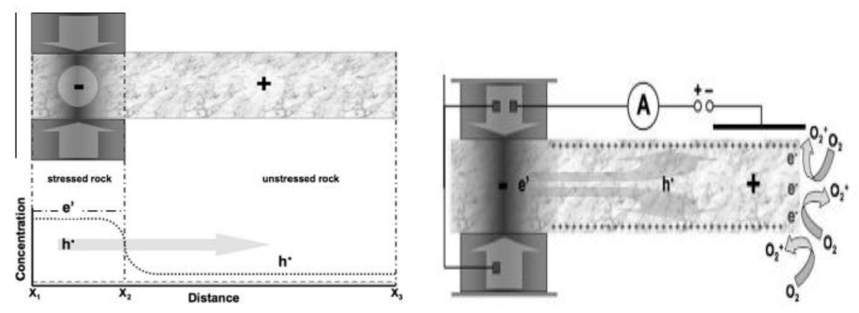
Figure 2.
Seismic Lights during the Large Mexico 7.0 M EQ (First and Second photos from the left) and Maroc 6.8 Μ EQ (last photo to the right.). EQ lights (EQLs) were long ago considered as unexplained exotic phenomena, that heightened public fear during EQs.
Figure 2.
Seismic Lights during the Large Mexico 7.0 M EQ (First and Second photos from the left) and Maroc 6.8 Μ EQ (last photo to the right.). EQ lights (EQLs) were long ago considered as unexplained exotic phenomena, that heightened public fear during EQs.
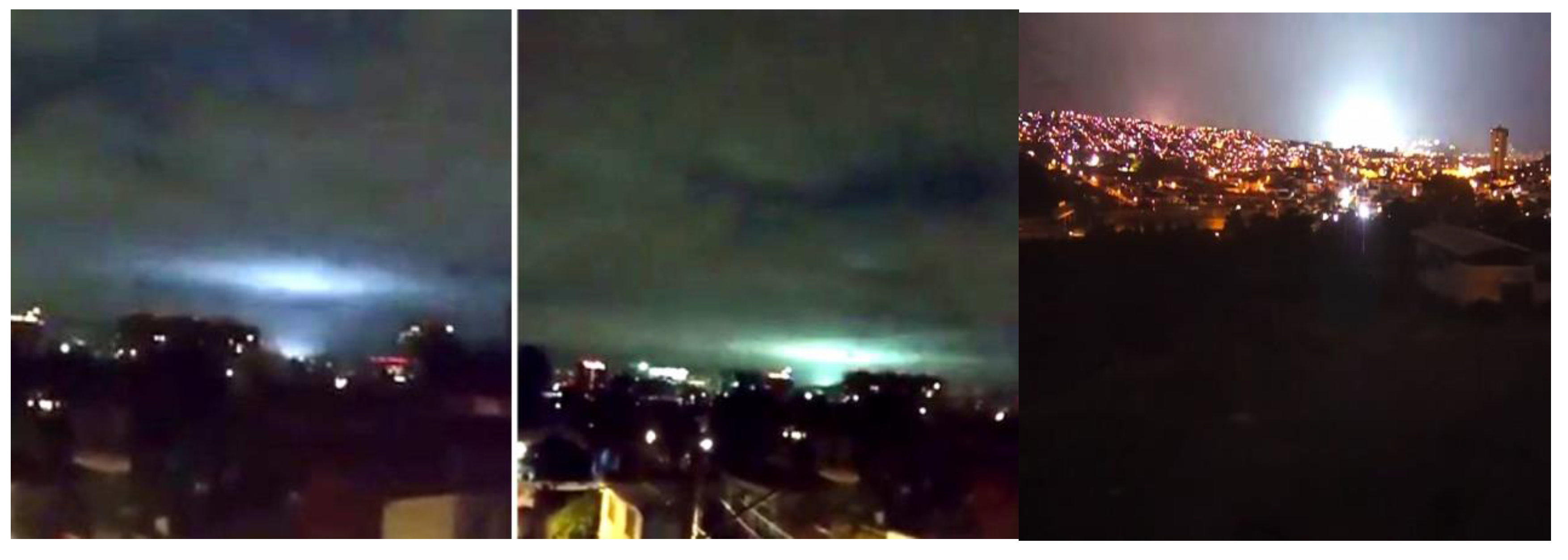
Figure 3.
-A flow chart of the first LAIC scenario by Pulinets and Ouzounov (2010), Journal of Asian Earth Sciences 41, 371–382.
Figure 3.
-A flow chart of the first LAIC scenario by Pulinets and Ouzounov (2010), Journal of Asian Earth Sciences 41, 371–382.
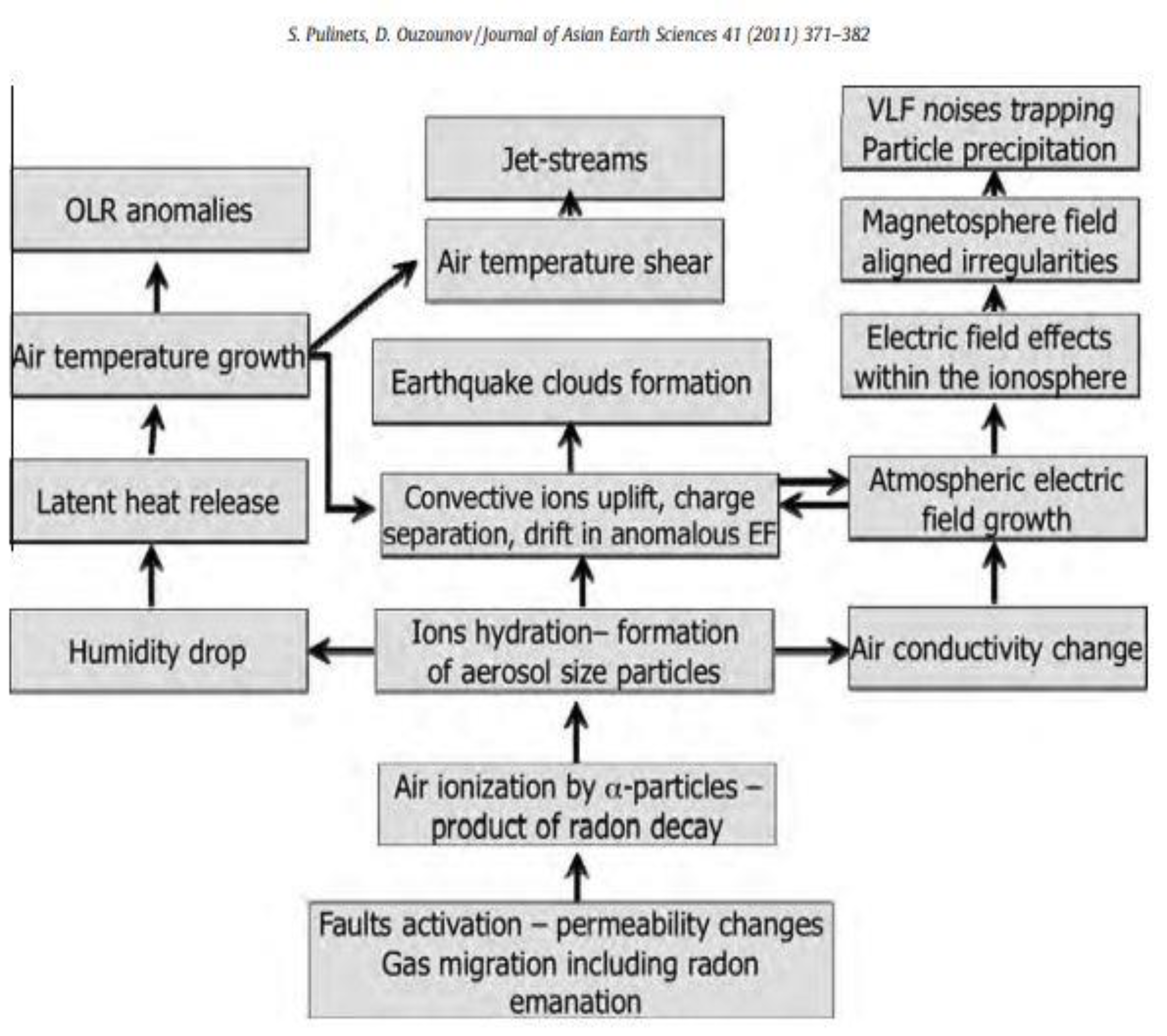
Figure 4.
A detailed presentation of the LAIC scenario where most of the known interactions between the Lithosphere and the Ionosphere have been depicted. (From Hayakawa et. al. (2019). International Journal of Electronics and Applied Research (IJEAR)vol. 6, issue 2, Dec Online (http://eses.net.in/online_journal.html).
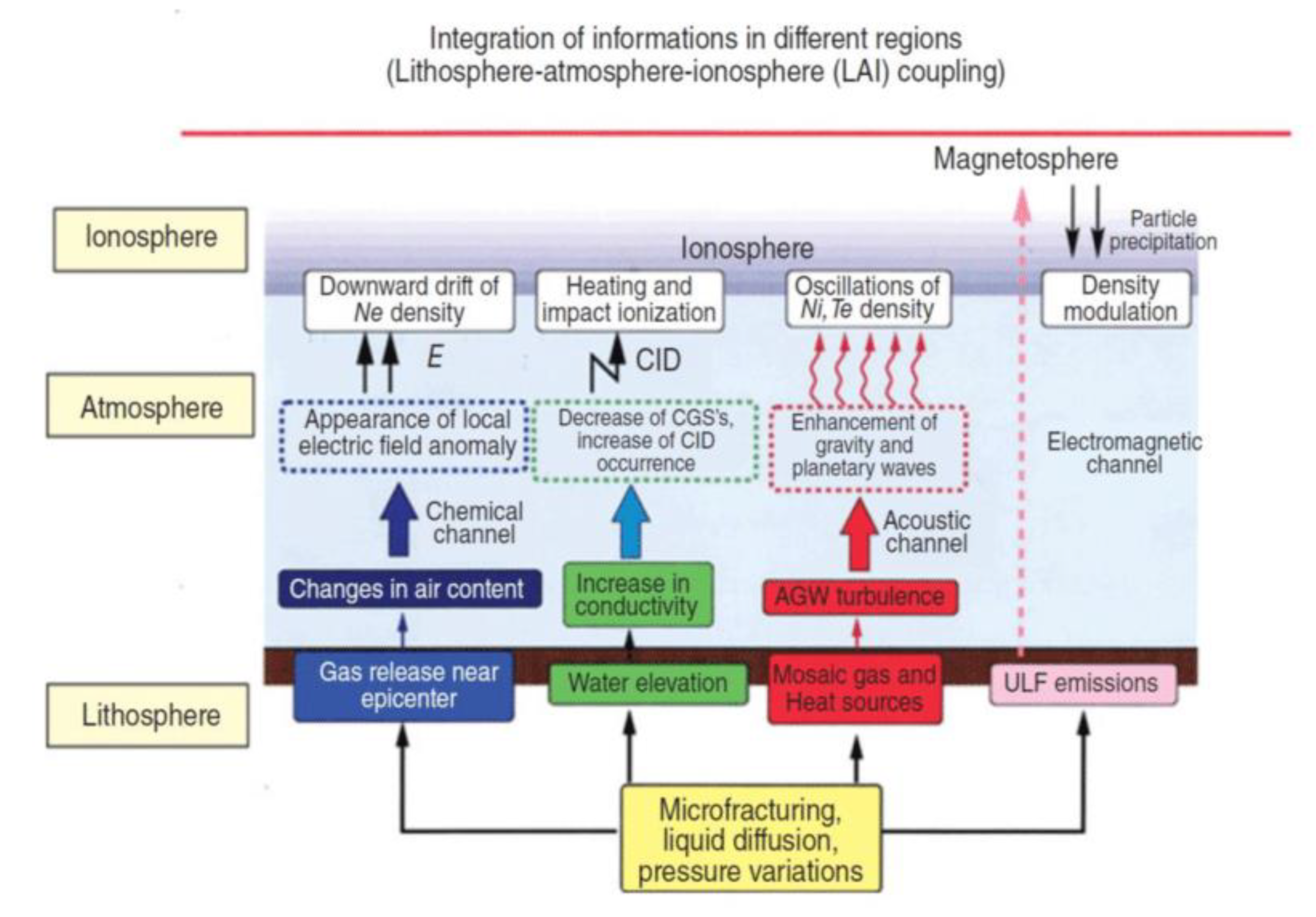
Figure 5.
Representation of undersea EQ- atmospheric-ionospheric-coupling where Infrasonic Acoustic Waves (IAWs), Acoustic Waves (Aws) and Acoustic Gravity Waves (AGWs) participate in the LAIC interactions (fig.5a). In the side figure (5b) Randon emanation from the sea-bottom which possibly contributes to atmospheric thermal anomalies which may create atmospheric oscillations and trigger Acoustic Gravity Waves (AGW). (From Dan Tao et.al. remote sensing 14, preprint).
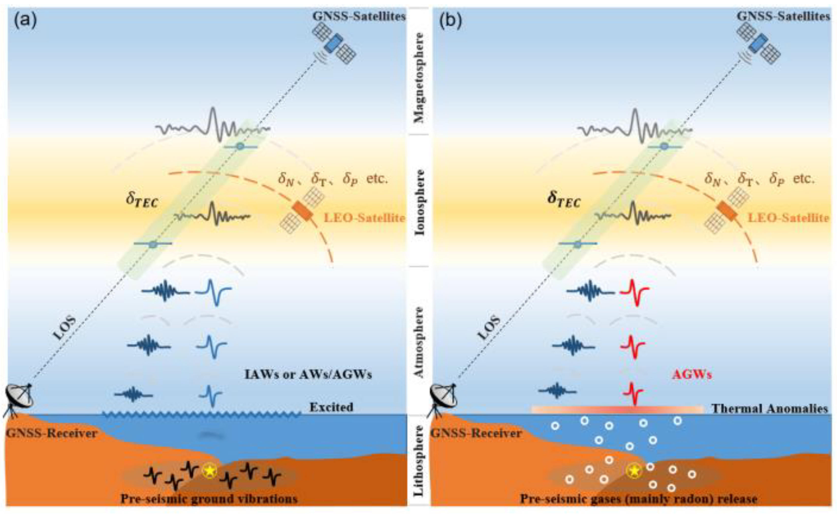
Figure 6.
Typical ELF recordings 0-50 Hz, raw data (upper panels) and associated Fourier spectra (low panels), received by both a Greek (left) and a Polish (right) system in an observing site on Mount Parnon in South Greece. Schumann’s Resonances around 7, 14, 21, and 28 Hz are evident in both spectra. PSD stands for “Power Spectral Density” in the Greek system recording (left). ASD stands for “Auto-Spectral Density” in the Polish system recording (right).
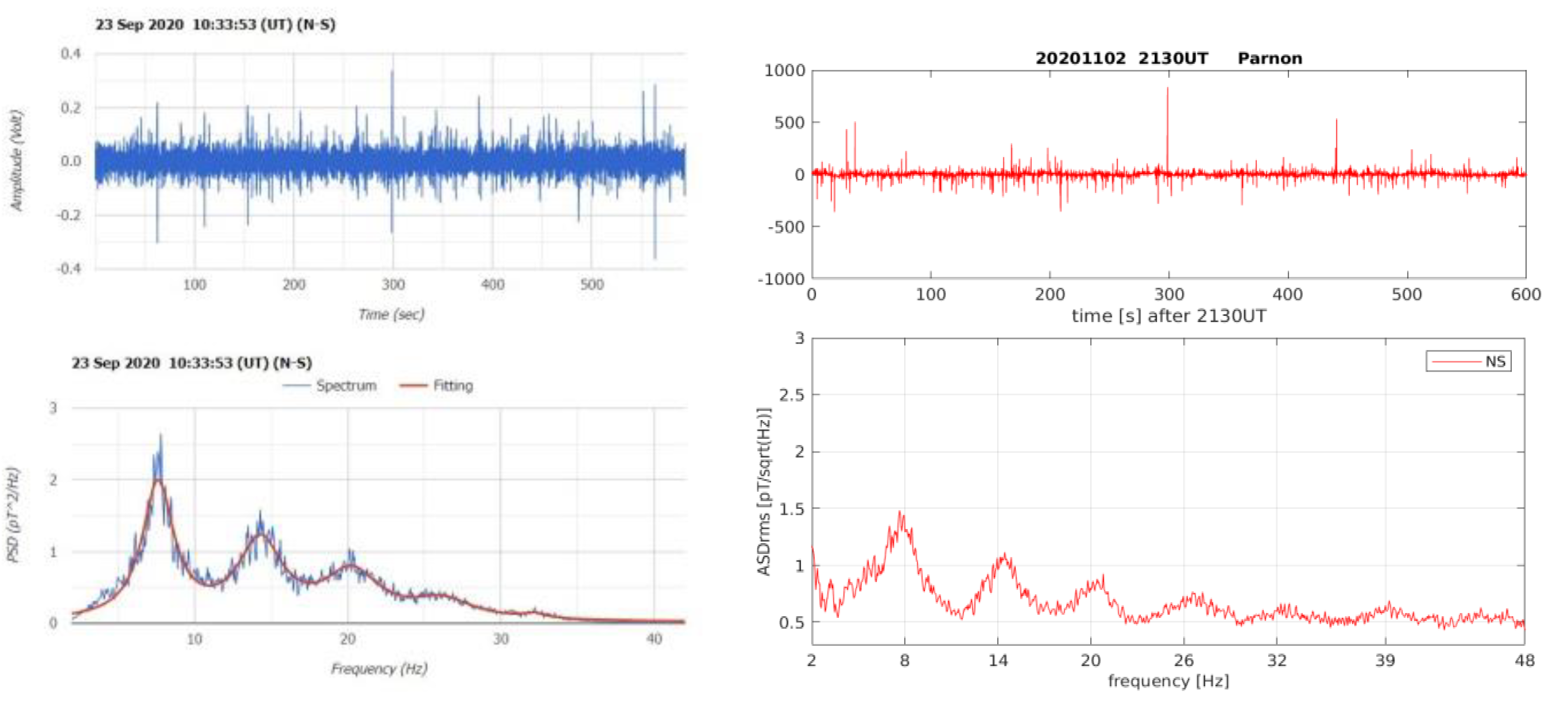
Figure 7.
Typical quasi preseismic signals recorded by the Greek (left) and the Polish systems (right) ten days before an EQ of 5,0 R which occur in the sea area of the Greek island Hydra.
Figure 7.
Typical quasi preseismic signals recorded by the Greek (left) and the Polish systems (right) ten days before an EQ of 5,0 R which occur in the sea area of the Greek island Hydra.
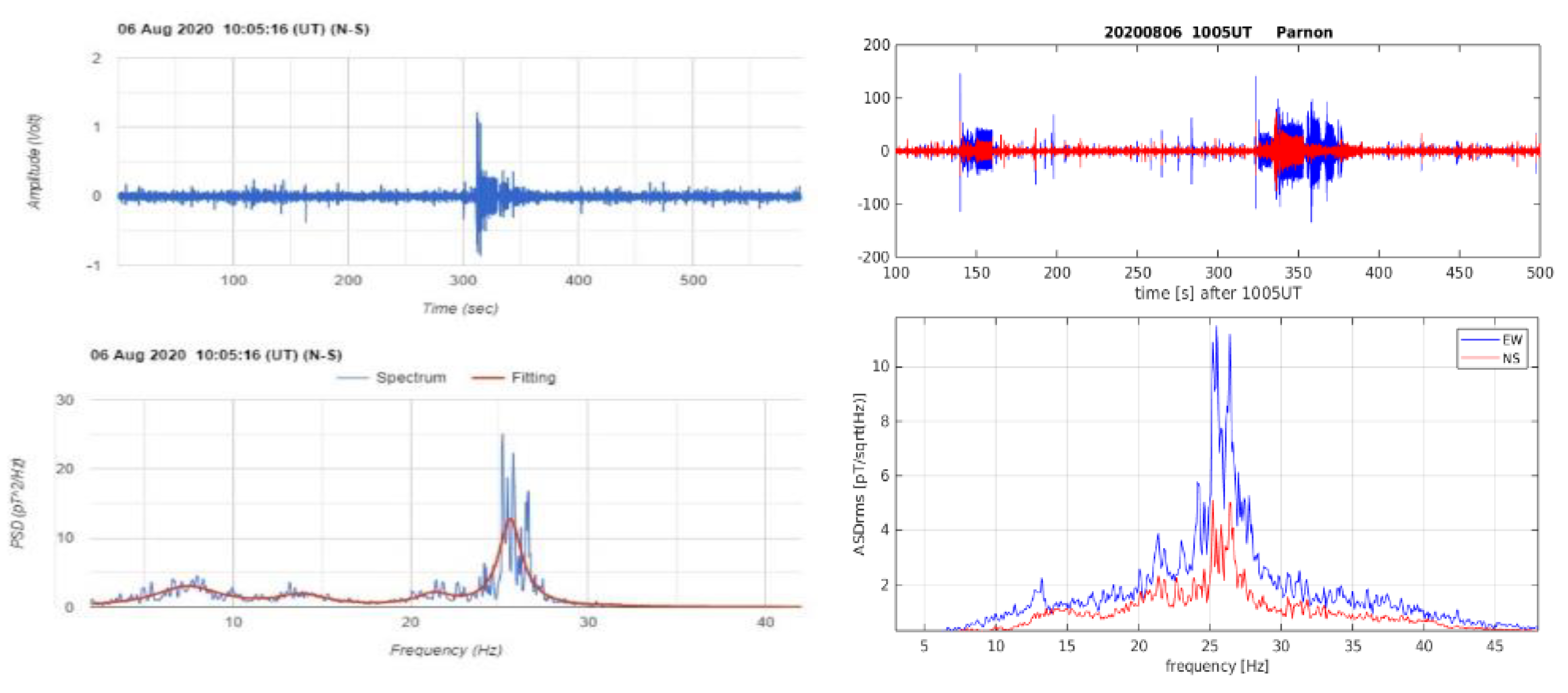
Disclaimer/Publisher’s Note: The statements, opinions and data contained in all publications are solely those of the individual author(s) and contributor(s) and not of MDPI and/or the editor(s). MDPI and/or the editor(s) disclaim responsibility for any injury to people or property resulting from any ideas, methods, instructions or products referred to in the content. |
© 2025 by the authors. Licensee MDPI, Basel, Switzerland. This article is an open access article distributed under the terms and conditions of the Creative Commons Attribution (CC BY) license (http://creativecommons.org/licenses/by/4.0/).
Copyright: This open access article is published under a Creative Commons CC BY 4.0 license, which permit the free download, distribution, and reuse, provided that the author and preprint are cited in any reuse.


