
Submitted:
08 March 2025
Posted:
12 March 2025
You are already at the latest version
Abstract
Deep learning models have shown great potential in scientific research, particularly in remote sensing, for monitoring natural resources, environmental changes, land cover and land use. Semantic segmentation techniques enable land cover classification, change detection, object identification, and vegetation health assessment, among other applications. However, their effectiveness relies on large labeled datasets, which are costly and time-consuming to obtain. Domain adaptation (DA) techniques address this challenge by transferring knowledge from a labeled source domain to one or more unlabeled target domains. While most DA research focuses on a single target domain, multi-target and multi-source scenarios remain underexplored. This work proposes a deep learning approach that uses Domain Adversarial Neural Networks (DANN) for deforestation detection in multi-domain settings. Additionally, an uncertainty estimation phase is introduced to guide human review in high-uncertainty areas. Our approach is evaluated on Landsat-8 images from the Amazon and Brazilian Cerrado biomes. In multi-target experiments, a single source domain contains labeled data, while samples from the target domains are unlabeled. In multi-source scenarios, labeled samples from multiple source domains are used to train the deep leraning models, later evaluated on a single target domain. The results show significant accuracy improvements over lower-bound baselines, as indicated by F1-score and mean Average Precision (mAP) values. Furthermore, uncertainty-based review showed a further potential to enhance performance, reaching upper-bound baselines in certain domain combinations.
Keywords:
deforestation detection
; domain adaptation
; multiple target domains
; multiple source domains
; uncertainty estimation
; deep learning
1. Introduction
Deforestation, is a critical environmental problem that currently attracts the attention of researchers, policy makers, and the general public. The problem is particularly important in tropical regions, where high rates of deforestation have led to significant losses of biodiversity, also contributing to global climate change [1]. Numerous studies have investigated the causes of deforestation, as well as proposed solutions to mitigate its expansion. Laurence et al. [2] identifies key drivers of deforestation in the Brazilian Amazon, including population growth, industrial activities, road construction, and human-induced wildfires. According to Barber et al. [3], deforestation in the Amazon forest is strongly associated with proximity to roads and rivers, while protected areas help to prevent it. Colman et al. [4], on the other hand, argue that the rate of deforestation in the Cerrado has been historically higher than in the Brazilian Amazon, being the conversion of native vegetation areas in agriculture over the last 30 years the main driver of these changes. Given their crucial role in global climate stability, addressing deforestation is essential for protecting such unique ecosystems and safeguarding the planet’s well-being.
Fortunately, advances in remote sensing technology have improved monitoring capabilities. Hansen et al. [5] mapped global forest loss, finding tropical regions, including the Amazon, the most affected. In this regard, among other initiatives, the PRODES project stands out as a key program for monitoring deforestation in Brazil. Developed by the Brazilian Space Research Institute (INPE), it uses optical satellite data to track deforestation in the Brazilian Amazon and other biomes, providing reliable information on deforestation trends, aiding environmental management.
Jiang et al. [6] highlights that deep learning (DL) techniques have recently become a leading approach in various fields, including remote sensing. Nonetheless, DL models typically need extensive labeled datasets to be trained, and producing such reference data is expensive and time-consuming, demanding field surveys and expert image interpretation. Additionally, environmental dynamics, geographical differences, and sensor variations restrict the application of pre-trained classifiers to new data, leading to reduced accuracy. These challenges exemplify what is called as the domain shift, when source domain data marginal distribution differs substantially from the one of the target domain. Domain shift as well as the high demand for labeled training data hampers the implementation of broad scale, real-world, DL-based remote sensing applications.
When considering deforestation as a single process, it is necessary to include not only the extremes of the process, like clear-cutting, which are more obvious and easier to identify, but also the forest degradation gradient that occurs throughout the deforestation process. This degradation can occur slowly over time due to continuous logging and successive occurrences of forest fires. Despite various classifications found in other literature, the methodology employed by PRODES [7] condenses the distinct types of deforestation into the two above-mentioned main categories, i.e., clear-cutting and degradation.
As documented by IBGE [8], the predominant vegetation in the Amazon is the dense ombrophilous forest, which represents 41.67% of the biome. This type of forest is densely wooded, with tall trees, a wide range of green hues, and high rainfall (less than 60 dry days per year). Another type of vegetation present is the open ombrophilous forest. It features vegetation covered with palm forests throughout the Amazon and even beyond its borders, along with bamboo in the western part of the Amazon. Unlike the dense ombrophilic forest, it has lower rainfall. In the Brazilian Cerrado biome, there is a mixture of forest, savanna, and grassland formations. The biome is characterized by scattered trees and shrubs, small palms, and a grass-covered soil layer [9].
The distinct differences among various biomes pose a significant challenge for DL models when applied to deforestation detection. Rainforests, savannas, and grasslands, exhibit unique ecological characteristics, including diverse types of vegetation, terrain variations, and weather patterns. These variations introduce considerable variability in the visual features present in satellite images, making it difficult for a model trained on one biome to generalize effectively to others.
In this study, our focus is on imagery from two distinct Amazonian locations, Pará (PA) and Rondônia (RO), and one site situated within the Cerrado biome, Maranhão (MA). Each site exhibits distinct patterns of deforestation, characterized by varying distributions of deforestation types. According to [10], clear-cutting with exposed soil is the predominant form of deforestation in Pará, Rondônia, and Maranhão. However, the extent of this practice varies significantly across those regions. In Maranhão, clear-cutting with exposed soil is dominant. In contrast, Pará and Rondônia show a more balanced distribution, with significant contributions from progressive degradation with vegetation retention. Additionally, Pará stands out for having a small but noteworthy proportion of deforestation attributed to mining activities.
Several studies have explored domain adaptation (DA) methods for deforestation detection from remote sensing data. Soto Vega et al. [11] proposed an unsupervised DA approach based on the CycleGAN [12], which transforms target domain images, so that they resemble source domain images while preserving semantic structure. Noa et al. [13] introduced a domain adaptation method based on Adversarial Discriminative Domain Adaptation (ADDA) [14] for semantic segmentation, which incorporates a domain discriminator network during training. Soto et al. [15] developed a DA method derived from Domain-Adversarial Neural Networks (DANN) [16], integrating change detection and patch-wise classification, and employing pseudo-labels to address class imbalance. Vega et al. [17] introduced the Weakly-Supervised Domain Adversarial Neural Network method for deforestation detection, which uses the DeepLabv3+ architecture [18]. This approach uses pseudo-labels both for dealing with class imbalance, and for a form of weak supervision to enhance the accuracy of domain adaptation models.
While those methods demonstrated effectiveness in single-source, single-target settings, none of them addressed multi-source or multi-target scenarios in a semantic segmentation task, a gap that this study aims to fill. In terms of uncertainty estimation, Martinez et al. [19] evaluated uncertainty estimation techniques and introduces a novel method to improve deforestation detection. By integrating uncertainty estimation into a semiautomatic framework, the approach flags high-uncertainty predictions for visual, expert review. This study provided a strong foundation for this work, reinforcing the use of predictive entropy from an ensemble of DL models.
The method introduced in this work aims at tackling the above-mentioned problems in the context of deforestation detection with deep learning models, in a partially assisted strategy. We propose a two-phase approach, called Dense Multi-Domain Adaptation (DMDA). In the first phase, extending the Domain Adaptation Neural Networks (DANN), a pixel-wise classifier is trained using the a particular DL architecture, combined with DA techniques to enable unsupervised training for deforestation prediction across different target domains. In the multi-target setting, a single labeled source domain is used to adapt to multiple unlabeled target domains. In the multi-source DA setting, the method adapts from multiple labeled source domains to a single unlabeled target domain.
In the second phase, following the method proposed by Martinez et al. [19], the prediction of the model is supplemented by expert auditing, focusing on areas with high uncertainty, determined by an uncertainty threshold. The predictions for each pixel in the target domain are used to calculate the entropy, which is used to identify high-uncertainty regions for further human visual inspection. Once this inspection is completed, we assume that the predictions for the selected areas of high uncertainty are accurate, and we recalculate recall, precision, and F1 score metrics values. The hypothesis is that the use of DA methods combined with uncertainty estimation not only improves the accuracy of the deforestation predictions in unseen domains, but also provides users with greater transparency in the reliability of the models, as well as the opportunity to manually improve its overall performance, recommending the most uncertain areas for visual inspection.
The main contributions of this work are as follows:
- Two distinct scenarios of domain adaptation (DA) are presented. The first, termed multi-target, involves a single source domain and multiple target domains. The second, known as multisource, consists of multiple source domains adapting to a single target domain.
- Two configurations of the domain discriminator component were evaluated: multi-domain discriminator and source-target discriminator.
- Inclusion and assessment of an expert audit phase designed to target areas of highest uncertainty, utilizing uncertainty estimation from the predictions made by the DL model in a domain adaptation context.
- Experiments are conducted in three different domains associated with Brazilian biomes, and our approach is validated by comparing the results obtained with single-target and baseline experiments.
The remainder of this document is organized as follows. Next section presents materials and methods. Then, in Section 3, we present the experimental procedure, while Section 4 is dedicated to results presentation. Finally, Section 5 is dedicated to results discussion, while Section 6 presents the conclusions.
2. Materials and Methods
2.1. Domain Adversarial Neural Network (DANN)
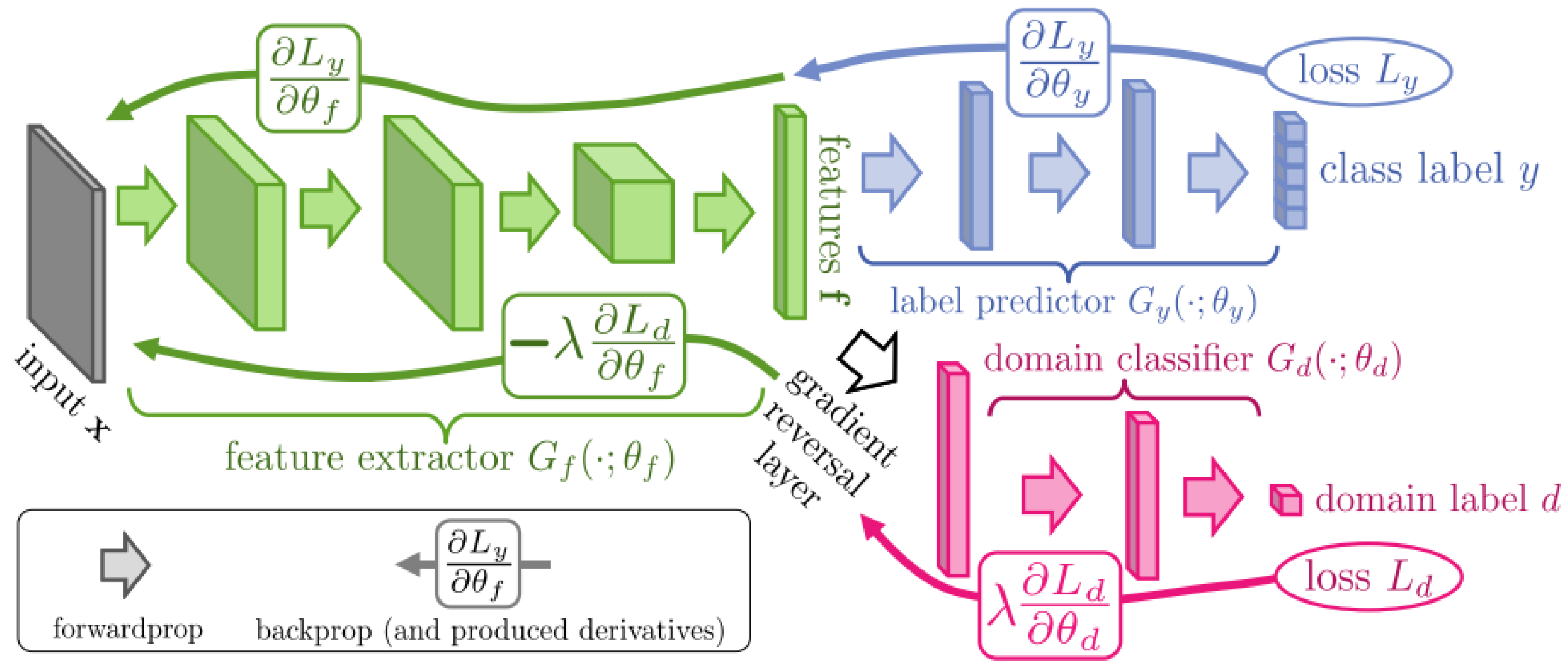
Proposed in [16], DANN aims to minimize the divergence between two probability distributions by learning domain-agnostic latent representations employing adversarial training. As depicted in Figure 1, three modules compose the DANN strategy: a feature extractor , a label predictor and a domain classifier . In short, maps both the source and target learned features into a common latent space, estimates the input sample categories, and , used only during training, tries to discern between source and target samples from the features given by .
In the DANN domain adaptaion startegy, does not evaluate features coming from target domain samples, as their corresponding labels are unknown. In contrast, source and target domain features are forwarded through , as their domain labels are known. The optimal network parameters , and are given by Equations (1) and (2):
where represents the DANN loss function defined by:
The first term of the loss function represents the label predictor loss, and the second term is the domain classifier loss. The coefficient controls the influence of the domain classifier over the feature extractor parameters. In [16], the authors suggest that should start and remain equal to zero during the first epochs allowing the domain classifier to properly learn how to discern among features of the respective domains. Afterwards, the coefficient value gradually increases through the training epochs favoring the domain classifier influence to the feature extractor in the opposite direction. As a result, the learning process updates the parameters of the model by implementing the rules detailed in Equations (4), (5) and (6). We observe that and in the aforementioned equations are both positive. Therefore, the derivatives of push and in opposite directions, configuring an adversarial training, which is expressed by the last term of Equation (6).
This term penalizes when correctly identifies the domain to which an input sample belongs. DANN implements such an operation on Gradient Reversal Layer (GRL) (see Figure 1). Summarily, during the forward procedure, the GRL acts as an identity mapping and, during the backpropagation, reverses the gradient (multiplying it by ) coming from the domain classifier.
Figure 1.
DANN proposed architecture (source: [20]).
Figure 1.
DANN proposed architecture (source: [20]).
2.2. Dense Multi-Domain Adaptation
This work proposes an approach called Domain Adversarial Neural Network Dense Multi-Domain Adaptation (DANN-DMDA) to tackle the challenges of deforestation detection by exploring two settings. In the first, termed Multi-Target DA, a set of a labeled source domain is incorporated alongside multiple sets of unlabeled target domains combined into a single one for adaptation. In the second setting, known as Multi-Source DA, we combine multiple labeled source domains into a single one to adapt to a single unlabeled target domain. The hypothesis is that utilizing domain adaptation with multiple unlabeled target domains or multiple labeled source domains can improve the accuracy of deforestation prediction across these domains. Using both diverse target and source domains, the model can learn a more robust and generalized feature representation.
This work builds on the method proposed by [21], which introduced an unsupervised domain adaptation approach for deforestation detection. Additionally, the Deeplabv3+ semantic segmentation architecture was employed, as evaluated in [22] (please refer to Figure 4).
Like DANN, the DANN-DMDA approach employs two adversarial neural networks: the domain discriminator and the label predictor. The architecture includes an encoder model that transforms input samples into a latent representation, a decoder responsible for semantic segmentation, and a domain discriminator that attempts to classify the domain of the encoder’s output (determining whether it belongs to the source or target domain). In the Multi-Target configuration, the encoder component receives a set of labeled samples from one source domain and unlabeled samples originating from two or more distinct target domains. Alternatively, in Multi-Source setting, the encoder is provided with labeled samples from two or more source domains, and unlabeled samples from a single target domain.
By employing such an architecture and training methodology, we aim to obtain a common feature representation shared across all domains involved, and thus improve the performance of semantic segmentation on each target domain. Although our method can be generalized to multiple target domains, we make use of two targets only to showcase the method and experiments.
Figure 2 and Figure 3 illustrate in a simplified way the blend of target and source samples for domain adaptation.
The proposed method follows the general structure outlined by [21], which consists of three phases: data pre-processing, training, and evaluation.
First, there is a data pre-processing phase, which consists of the following procedures. The first is to apply the Early Fusion (EF) procedure, that concatenates images taken at different periods of time in the spectral dimension. Then, each image is partitioned into tiles, which are then allocated to training, validation, and test sets. From each tile, small patches are extracted to be used as input to the DANN-DMDA model.
The training phase comes in sequence. We define two distinct designs for the domain classifier model. In the first, called the multi-domain discriminator, the discriminator label space is , where each class is represented by a unique value. In the other design, named source-target discriminator, the label space is , where 0 denotes the source domain, and 1 represents the target domain. In this case, there is no discrimination between specific source or target domains. For the label predictor model, a pixel-wise weighted cross-entropy loss is adopted in order to enable a calibration over of how much weight is given to no-deforestation and deforestation predictions. The domain discriminator model works with a cross-entropy loss.The DANN-DMDA model is trained until convergence by simultaneously updating the parameter sets .
2.3. Deep Learning Model Architecture
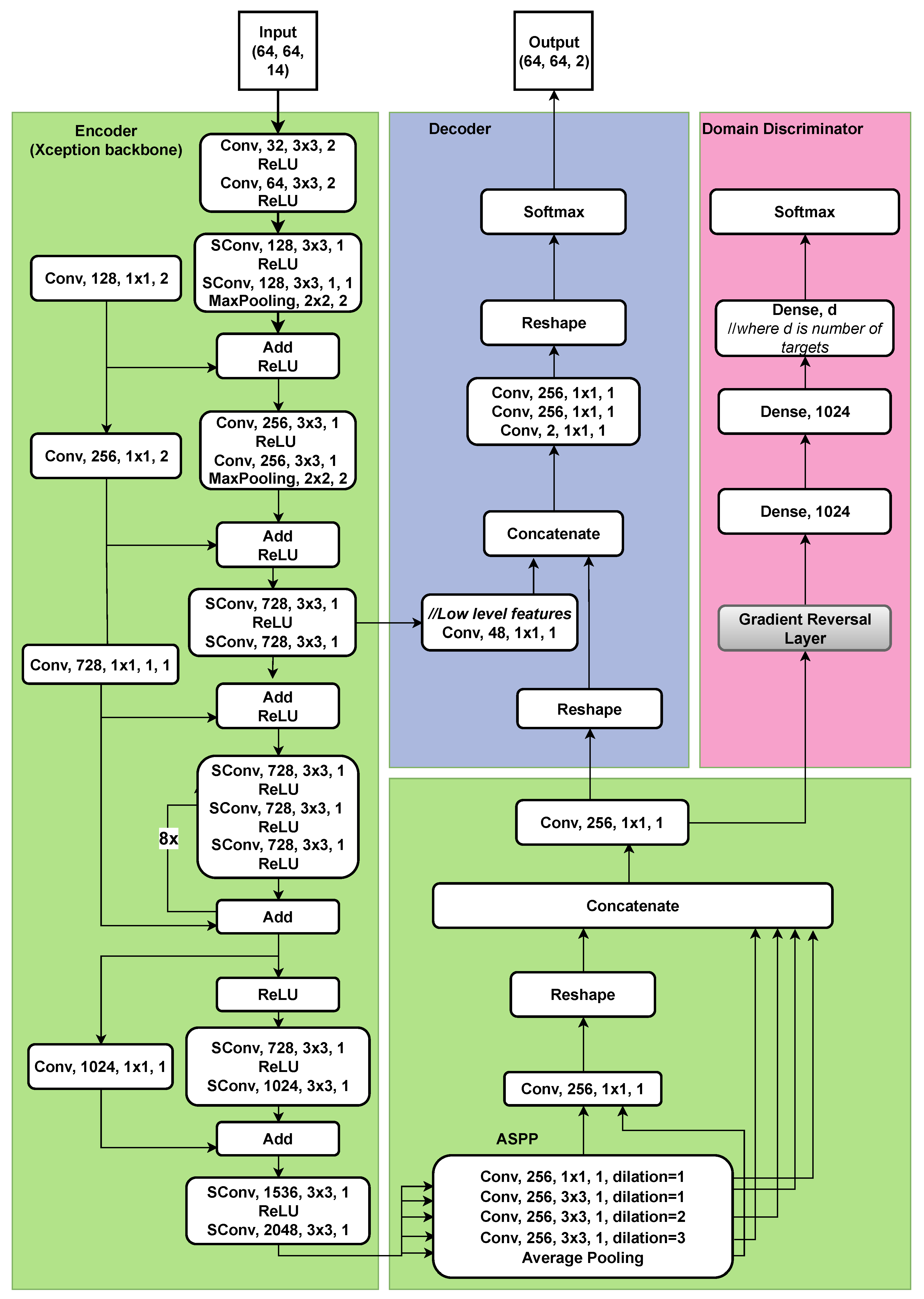
The DMDA model developed in this study extends an adapted version of the Deeplabv3+ architecture introduced in [17]. The encoder backbone relies heavily on Xception [23], although some adjustments have been made to adapt the network to the problem and the input data. The dilation rates of the atrous convolutions in the ASPP have been modified to 1, 2 and 3, replacing the original rates of 6, 12, and 18 [18].
Figure 4 provides a visual representation of the deep learning architecture. The layer descriptions include the following information: Convolution type ("Conv" for regular convolution; "SConv" means depthwise separable convolution), number of filters, filter size, and stride. In addition, the ASPP component displays dilation rate values.
Figure 4.
Overview of Deeplabv3+ architecture. The full model has over 54M trainable parameters.
2.4. Uncertainty Estimation
In the second phase, following [19], predictive entropy over an ensemble’s outcome is utilized as a metric for uncertainty estimation. The ensemble is composed of a set of instances of the architecture shown in Figure 4. Each instance is trained with different random initializations of network weights, and different batch selections, resulting in K different models. The uncertainty of the pixel-wise predictions is assessed by calculating the predictive entropy for the K models, as in Equation (7), in which is a model’s output probability map. In the following experiments K was arbitrarily chosen as five. The result is an uncertainty map with the same spatial dimensions as the prediction map.
To classify predictions as having high or low uncertainty, the uncertainty threshold Z is determined based on the audit area parameter , defined in terms of percentage of the total area. The uncertainty map values are sorted and the threshold Z is set at the percentile. The regions with high uncertainty are then selected for manual inspection. The goal is to find a threshold that optimizes the F1 score while minimizing manual review effort.
We adopted for samples with uncertainty below the threshold defined by the most uncertain pixels, which are subjected to audit. Contrarely, considers the pixels with the highest uncertainty values . represents the classification accuracy prior to auditing, and the classification performance after a human expert visually inspects and correctly annotates the high uncertainty regions. In this study, we simulate the inspection process by replacing the most uncertain pixels using their respective ground truth labels. It should be noted that this method of review of uncertainty areas can be applied to a model trained without domain adaptation as well, since it is independent of the training approach.
3. Experimental Protocol
3.1. Experiment Plan
This study included four types of experiments:
- Baselines: Validation of the deep learning architecture and establishment of reference benchmarks;
- DMDA Multi-target;
- DMDA Multi-source;
- Uncertainty Estimation with Review phase.
The architecture and domain adaptation (DA) methods were validated across various training and testing configurations. Regarding the baseline experiments, the models were evaluated by training and testing on the same domain (training on target), which serves as the upper-bound baseline, and by training on one source domain and testing on a different target domain (Source-only training), serving as the lower bound-baseline. Additionally, a single-target scenario was assessed to further validate the DA approach.
In order to verify the success of the proposed DANN-DMDA approach, multi-target, multi-source and uncertainty estimation experiments were conducted over all possible combinations of the three domains.
In each experiment, in the multi-target scenario, one domain dataset worked as source domain providing labels, whereas the other two domains were used as targetsAlternatively, in the multi-source setting, at each experiment two domains were used as sources, while another domain was used as target. For example, in the ’Source MA | Target PA’ combination, the RO domain was incorporated as an additional domain in DMDA experiments.
3.2. Datasets
The dataset, previously used in [17], consists of pairs of images from different sites within the Amazon and Cerrado biomes, located in the Brazilian states of Rondônia (RO), Pará (PA), and Maranhão (MA). The selected forest domains represent a range of forest types, from dense forests with slight variations in canopy structure to those with high variability. The class distribution is highly imbalanced in all domains. The images used were captured by the Landsat 8-OLI sensor, which has a 30x30-meter spatial resolution and seven spectral bands. They were downloaded from the USGS Earth Explorer website. The reference data on deforestation are freely available on the Terrabrasilis website1. All images were captured during July and August for optimal cloud coverage. Similar to [17], the image space of each domain was partitioned into tiles (large subsets of the images).
3.3. Model Training Setup
The image space within each domain was divided into tiles or large image subsets. Specifically, 100 tiles were defined for the RO image, while the PA and MA images were divided into 15 tiles each. For the RO tiles, approximately 20% were utilized for extracting training patches/samples, which are small image subsets matching the classifier input size; 5% of the tiles were assigned for extracting validation patches; and the remaining 75% were allocated for testing. In the case of the PA and MA images, 26% of the tiles were designated for training; 13% for validation; and 60% for testing. Table 2 and Figure 6 gives an overview of how the dataset has been organized.
Following data pre-processing, the domain patches are employed to train the proposed domain adaptation (DA) methods, whose settings and hyper-parameters are described next.
The extracted samples from image pairs across all domains consist of patches measuring 64 × 64 pixels, with 14 channels. Data augmentation techniques, including 90-degree rotation, as well as vertical and horizontal flips, were applied to the patches in both the source and target domains. In line with [21], we utilized the Adam optimizer and incorporated learning rate decay during the training process, whose formula is described in the Equation (8):
The initial learning rate was set to , while was assigned 10 and was set to 0.75. Here, p represents the training progress, which changes from 0 to 1, following the advance of the epochs.
The gradient reversal layer parameter is initially set to 0 and progressively updated over the epochs following the function defined in Equation (9). This scheduling strategy aims to gradually amplify the strength of gradient reversal during backpropagation from the domain discriminator, encouraging the feature extractor to learn more domain-invariant representations over time.
A batch size of 32 was employed, and an early stopping procedure was implemented to prevent overfitting. Moreover, following [25], for the loss functions, we set and to be a weighted cross-entropy function and a categorical cross-entropy respectively. During the training procedure, the model that was considered the best achieved both the lowest value for and the highest value for . This indicated strong performance on the primary task of deforestation prediction, while also ensuring that the encoder effectively fooled the discriminator, making it unable to distinguish the domain of the sample. The weights have been set to 2 and 0.4 for the deforestation and no-deforestation class respectively. This approach has been employed to address the issue of the highly imbalanced distribution between deforestation and no-deforestation pixels.
3.4. Hardware and Configuration
The DANN model and Deeplabv3+ were implemented in Python on top of Tensorflow2 1.15, which is an open-source library widely used for machine learning and deep learning tasks. The experiments were run on an 64-bit Ubuntu Linux machine, with 128 Gibibytes (GiB) of RAM and NVIDIA GeForce RTX 3090 with 24 GiB of graphics memory. The source code is hosted on Github: https://github.com/LPG-Uerj/FC-DANN_DA_For_CD_MultiTarget_TF2.
3.5. Metrics
The models were evaluated through the semantic segmentation of the input images. In this approach, each pixel within the input image provided to the network was assigned to one of two classes: deforestation or non-deforestation. Due to the significant class imbalance in the dataset, where deforested areas represent only a small fraction of the total, global accuracy is not among the most appropriate metrics for evaluating that models. To evaluate the performance of the classifiers in each scenario, the average F1-score (Equation (10)), mean average precision (mAP), precision (Equation (11)) and recall (Equation (12)) were calculated.
These metrics focused on the positive (deforestation) class obtained in each classifier trial. The F1-score was determined by computing the harmonic mean of the Precision and Recall values, as shown below on Equation (10):
where
In Equations (11) and (12), the number of true positives (TP) represents the pixels correctly assigned to the deforestation class, while the number of false positives (FP) corresponds to the pixels mistakenly classified as deforestation. The false negatives (FN) indicate the number of pixels that were incorrectly classified as non-deforestation.
To ensure comparability with previous studies, Recall, Precision and F1-Score metrics were calculated using a standard threshold of 0.5 for predictions. Probabilities below 0.5 were classified as non-deforestation, while those above were classified as deforestation. The mAP metric measures the area under the curve obtained by computing pairs of Precision and Recall values for different classification thresholds in the range of 0 to 1. This is calculated over the average of probability maps obtained from each classifier execution.
4. Results
4.1. Baseline and Multi-Target Results
Table 3 presents the Baseline along with Multi-Target results, highlighting the best outcomes for each Source-Target combination. DMDA Multi-Target experiments generally outperformed both Single-Target DA and Source-Only training. The Multi-Target Multi-Domain Discriminator achieved the highest mAP and F1-score in ‘Source PA | Target MA,RO | Test RO’ and ‘Source RO | Target MA,PA |Test PA’ combinations, while the Multi-Target Source-Target Discriminator performed best in ‘Source RO | Target MA,PA | Test MA’ and ‘Source MA | Target PA,RO | Test PA’. Both DMDA setups reversed the negative transfer observed in Single-Target DA for ‘Source RO | Target MA’. However, Single-Target DA was optimal for ‘Source MA | Target RO’, indicating that adding PA did not enhance accuracy. These results suggest that multi-target training can reduce domain-shift in an unsupervised target scenario. The Multi-Domain Discriminator generally outperforms the Source-Target Discriminator, except in the ‘Source RO | Target MA,PA | Test MA’ and ‘Source MA | Target PA,RO | Test PA’ cases, which warrants further investigation.
4.2. Multi-Source Results
In the Multi-Source setting, two domains were combined as sources (i.e., containing class labels), while a third served as the target domain. Three Multi-Source experiments were conducted: (i) Multi-Source only training, where no domain adaptation was applied; (ii) DMDA Multi-Source Multi-Domain Discriminator; and (iii) DMDA Multi-Source Source-Target Discriminator, both of which incorporated domain adaptation.
Table 4 highlights key findings. First, DMDA methods consistently improved performance over Multi-Source only training, demonstrating its benefits even when using multiple source domains. Second, the Multi-Domain Discriminator outperformed the Source-Target Discriminator across most combinations, reinforcing patterns observed in multi-target experiments.
4.3. Overall Multi-Domain Results
This section compares model performance across Single-Target DA, DMDA Multi-Target, and DMDA Multi-Source. The Multi-Domain Discriminator was used in the latter two, given its superior performance in most experiments. Results are analyzed against both lower- and upper-bound baselines.
Figure 7 illustrates results for target MA, where combining PA and RO as sources significantly improved F1-score, nearing the upper bound of 78.8%. As for target PA (Figure 8), adding RO to ‘Source MA | Target PA | Test PA’ did not yield improvements, suggesting limited transferability between PA and RO. However, incorporating MA into ‘Source RO | Target PA | Test PA’ significantly enhanced adaptation on multi-domain scenarios. This pattern also appears in Figure 9, where including PA in ‘Source MA | Target RO | Test RO’ degraded performance, while adding MA to ‘Source PA | Target RO | Test RO’ multi-domain experiments led to substantial gains of F1-Score.
Overall, these findings reinforce the value of multi-target and multi-source DA, with the Multi-Domain Discriminator proving particularly effective in most configurations.
Table 5 synthesizes the contribution in terms of F1-score gain of a third domain in multi-domain methods. The second column, Single-Target DA compared to lower bound, shows the contribution of the target in the adaptation training compared to source-only training. Including the MA domain in the multi-domain training improved the model’s performance when tested on both the RO and PA domains. This improvement may be attributed to the high complexity of forested areas in that region, driven by greater environmental variability. The presence of prolonged dry periods throughout the year leads to natural vegetation loss not associated with deforestation.
Another key finding is that introducing PA as a third domain benefits the model when tested on MA (RO-MA) but degrades performance compared to the Single Target DA setting for MA-RO. A similar trend is observed with RO as the third domain: it enhances results in the Multi-Source experiment for PA-MA but remains comparable to Single Target DA for MA-PA, showing minor gains and losses in Multi-target and Multi-Source scenarios, respectively. This behavior may stem from the fact that PA and RO share a more homogeneous and dense forest structure, along with a higher proportion of progressive degradation, a more challenging feature to detect compared to the MA domain.

Table 5.
Comparative Analysis of Methods in terms of F1-Score. In the Domain Pairs column, ‘Source’ denotes the primary labeled domain used for training, while ‘Target’ represents the domain evaluated during testing. The third column, ‘Domain included in multi-domain Methods,’ specifies the additional domain which was incorporated in Multi-Target and Multi-Source experiments.
| Domain pairs (Source-Target) |
Single-target DA compared to lower bound | Domain included in multi-domain methods | DMDA Multi-Target Multi-Domain Disc. compared to Single-target DA | DMDA Multi-Source Multi-Domain Disc. compared to Single-Target DA |
|---|---|---|---|---|
| PA-RO | +10.9 | MA | +4.5 | +21.0 |
| RO-PA | +16.3 | MA | +0.6 | +10.5 |
| PA-MA | +8.6 | RO | -3.4 | +17.5 |
| MA-RO | +11.8 | PA | -0.6 | -6.3 |
| RO-MA | -5.7 | PA | +7.3 | +17.6 |
| MA-PA | -1.5 | RO | +0.5 | -1.2 |
4.4. Uncertainty Estimation with Review Phase Results
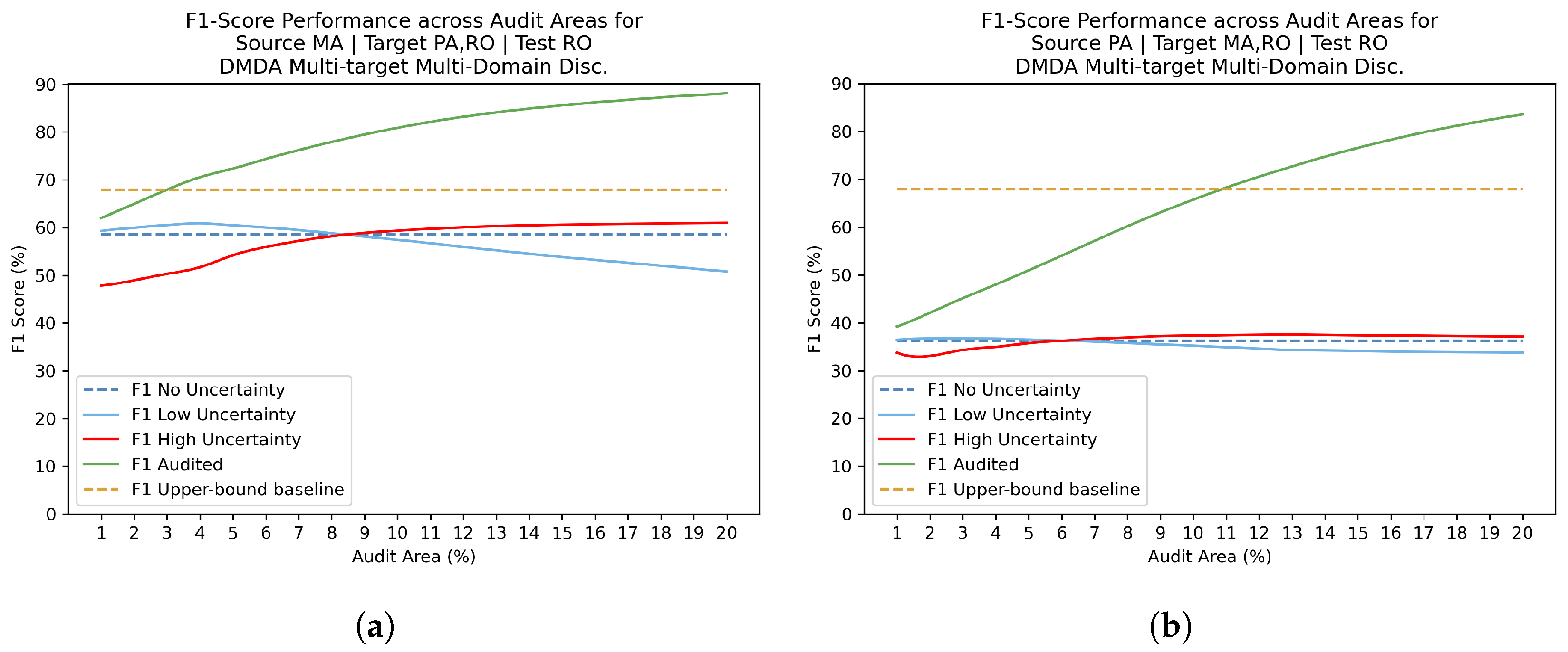
After domain adaptation training procedures, Uncertainty estimation with Review phase was included to the study. F1 scores were calculated for discrete audit area values ranging from 1% to 20%. Figure 10, Figure 11 and Figure 12 present the F1 score values in different scenarios: without uncertainty filtering, calculated only over low-uncertainty pixels, calculated over high-uncertainty pixels, and after applying the audit process. The observed pattern revealed that the F1 score for high uncertainty predictions consistently exhibited the lowest values, while the F1 score for low uncertainty predictions surpassed the original F1 score obtained without audit. This finding supports the hypothesis that strong F1 performance is associated with predictions characterized by low uncertainty. Nonetheless, Figure 12 reveals an intriguing observation: for the configurations Source MA | Target PA and Source RO | Target PA, the low-uncertainty and high-uncertainty lines intersect when the audit areas exceed 8% and 6%, respectively. This indicates that, for the RO target, larger audit areas diminish the effectiveness of the threshold in distinguishing between high and low uncertainties. This phenomenon may be attributed to the relative lack of regions predicted with high confidence in the RO domain compared to other target domains. Moreover, our findings reveal that surpassing the upper-bound baseline across all three domains is achievable by auditing at most 11% of the area, as can be seen in Figure 10 and Figure 12.
In most combinations, the F1 Audited curve shows its steepest increase between 1% and 5%, after which the this curve reaches its stability regime. To simplify the experiments and maintain comparability with [19], the audit area has been arbitrarily fixed as 3%, which offers a good balance between model performance and human effort required.
Figure 10.
Audit areas versus F1-score performance for MA target domain. The upper-bound baseline corresponds to the ’Training on Target’ experiment conducted on the MA target domain. (a) Source PA | Target MA,RO | Test MA. (b) Source RO | Target MA,PA | Test MA.
Figure 10.
Audit areas versus F1-score performance for MA target domain. The upper-bound baseline corresponds to the ’Training on Target’ experiment conducted on the MA target domain. (a) Source PA | Target MA,RO | Test MA. (b) Source RO | Target MA,PA | Test MA.
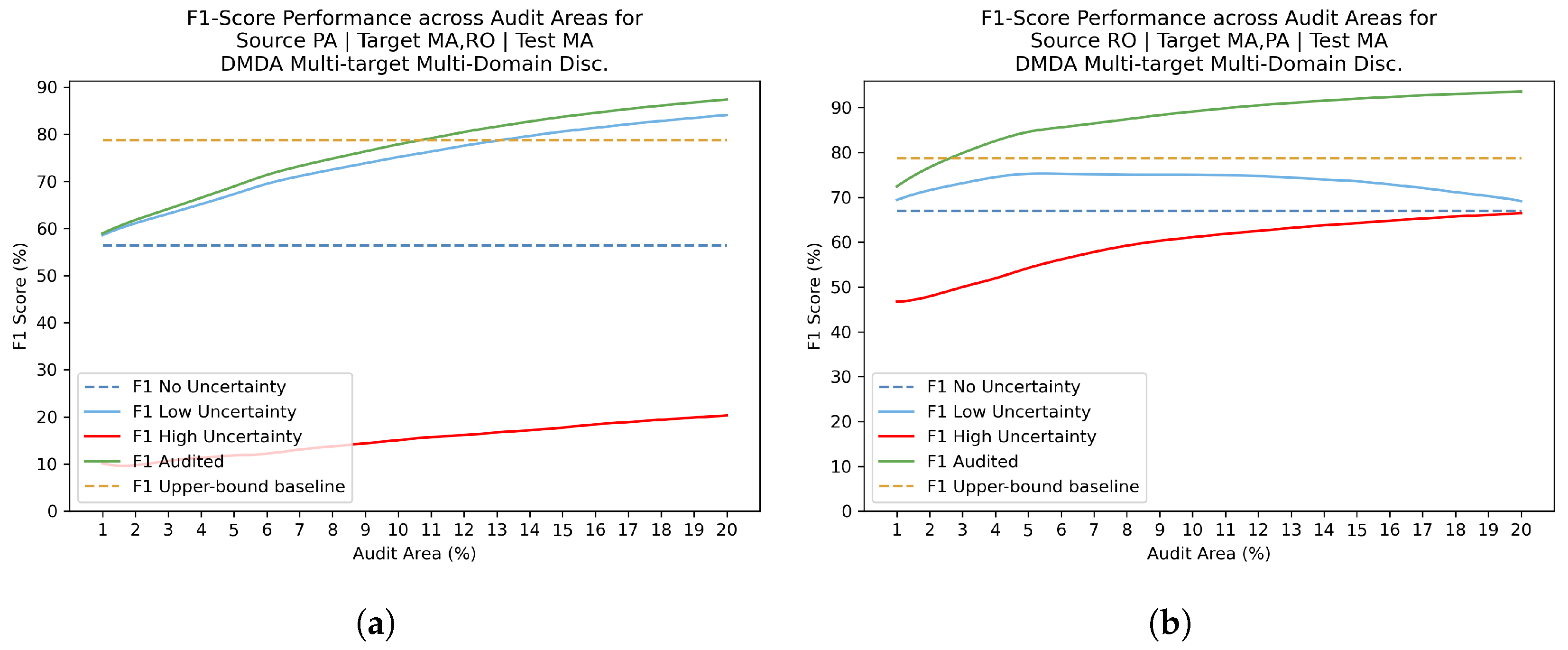
Figure 11.
Audit areas versus F1-score performance for PA target domain. The upper-bound baseline corresponds to the ’Training on Target’ experiment conducted on the PA target domain. (a) Source MA | Target PA,RO | Test PA. (b) Source RO | Target MA,PA | Test PA.
Figure 11.
Audit areas versus F1-score performance for PA target domain. The upper-bound baseline corresponds to the ’Training on Target’ experiment conducted on the PA target domain. (a) Source MA | Target PA,RO | Test PA. (b) Source RO | Target MA,PA | Test PA.
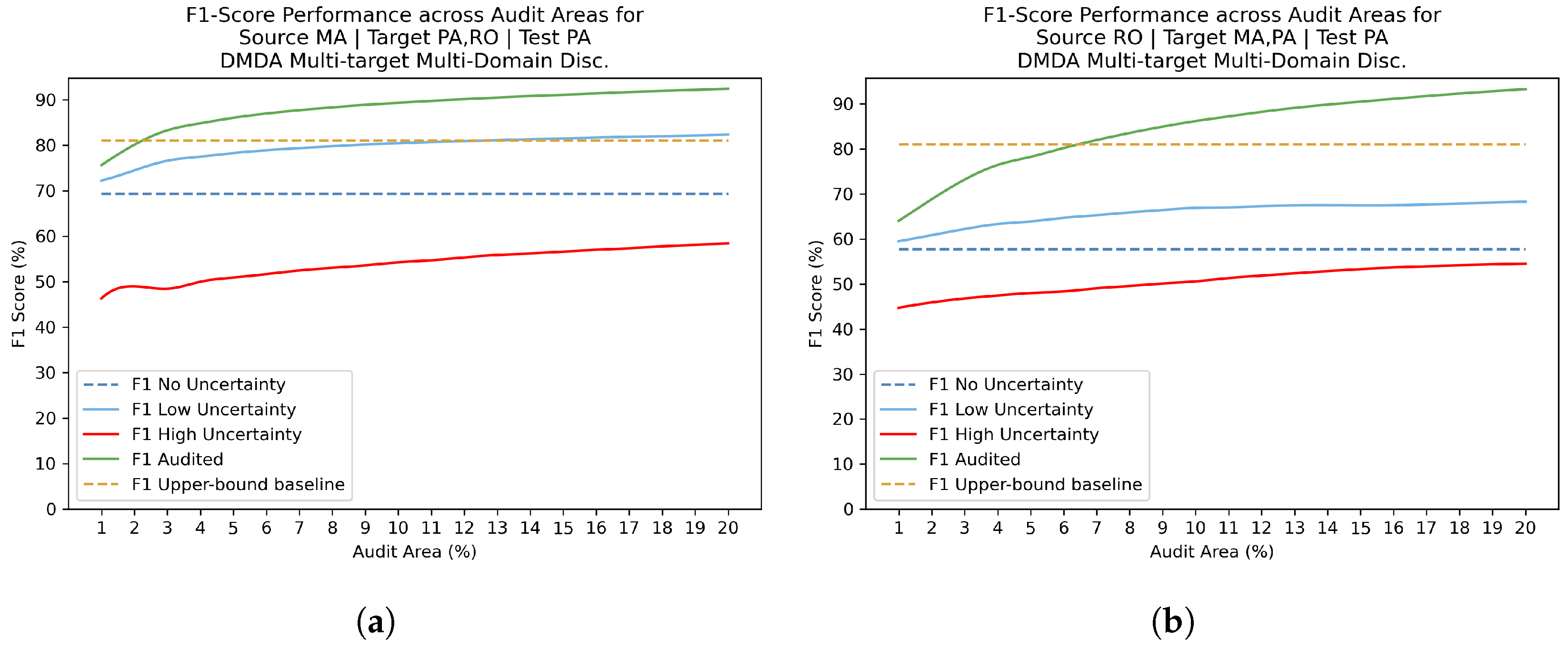
Figure 12.
Audit areas versus F1-score performance for RO target domain. The upper-bound baseline corresponds to the ’Training on Target’ experiment conducted on the RO target domain. (a) Source MA | Target PA,RO | Test RO. (b) Source PA | Target MA,RO | Test RO.
Figure 12.
Audit areas versus F1-score performance for RO target domain. The upper-bound baseline corresponds to the ’Training on Target’ experiment conducted on the RO target domain. (a) Source MA | Target PA,RO | Test RO. (b) Source PA | Target MA,RO | Test RO.
To maintain conciseness in the results presentation, uncertainty estimation was applied exclusively to the multi-target experiments. The quantitative results for the Uncertainty review are summarized in Table 6, Table 7 and Table 8. Consistent with the methodology used in previous experiments, the Training on Target experiment serves as the upper-bound baseline, where the model is trained and evaluated on the same domain. In contrast, the Source-Only Training experiment represents the lower-bound baseline, where the model is trained on one domain and tested on a different domain without utilizing domain adaptation techniques. As expected, in most experiments, the observed pattern was . Human inspections consistently improved model performance, as shown by the metric across all experiments, with results post-inspection correlating with pre-inspection outcomes. That is, when one of the the Multi-target experiments outperforms the Source-Only Training for example, this trend continues after auditing. In MA-PA combination, Table 6, post audit results outperforms the original F1 of the model trained on target (upper-bound baseline). In MA-RO source-target pair, DA Single target was also able to surpass the F1-Score from the upper-bound baseline. This outstanding result can also be seen on DMDA Multi-Target Multi-Domain Disc. experiment for RO-MA pair, in Table 8. In contrast, experiments based on PA source, Table 7, did not exceed the original F1-Score from upper-bound baseline, but produced improvements between six and ten points in terms of F1-Score.
5. Discussion
The results indicate that even with only one labeled source domain, prediction accuracy on a target domain can improve by incorporating an additional unlabeled target domain in the adaptation process. This inclusion helps the model learn features that are discriminative for the main task while remaining invariant to domain shifts. In the more favorable scenario of Multi-Source training, with two or more labeled source domains, the model significantly outperforms the lower-bound baseline and leverages the unlabeled data effectively, outperforming the ’Multi-Source only’ training experiment. This suggests that both multi-target and multi-source approaches are reliable methods to enhance model performance for deforestation detection. However, substantial gains with Multi-source and Multi-target domains heavily depend on the diversity of data attributes introduced by additional domains. Regarding the relationship among the three domains used in this study, the inclusion of Maranhão (MA) domain generally improves adaptation for the other domains. This may be explained by the higher complexity and variability of forested areas there. As MA has more dry periods, the visual characteristics of the forest changes without necessarily indicating deforestation. In addition, a model targeting MA is generally benefited from inclusion of PA or RO as third domain. Our hypothesis is that in areas with lower forest density, such as MA, the process of cleaning the area is easier and faster, resulting in more uniform deforestation footprints.
In contrast to other scenarios, the PA site presents a unique challenge due to its higher forest density. This density often results in incomplete deforestation processes, leaving behind debris that may persist for several years. As a consequence, these areas become visually harder to identify as deforested, complicating detection efforts. Both the PA and RO domains exhibit greater diversity in deforested areas, primarily due to the prevalence of clear-cutting with residual vegetation and regions undergoing progressive degradation. This diversity makes it more challenging to accurately classify these areas. When classifiers are trained on one domain (e.g., PA or RO) and applied to the other, they tend to produce a higher rate of false-positive predictions. In simpler terms, the PA and RO domains do not complement each other in terms of predictive accuracy, as the characteristics of deforestation in one domain do not translate well to the other.
Additionally, by using uncertainty estimation to refine predictions, the F1 score improved by 6 to 12 percentage points—a notable gain that, in some experiments, even exceeded the upper-bound baseline’s F1 score. The consistently low F1 scores in most metrics reveal a strong correlation between high uncertainty and prediction error.
6. Conclusions
The proposed approach learns invariant feature representations across multiple domains, whether source or target. This is achieved by strategically selecting samples from different domains and modifying the domain discriminator to predict the specific domain of each sample. Experimental results demonstrate that DMDA Multi-target outperformed Single-Target DA in four out of six cross-domain experiments. Furthermore, DMDA Multi-source surpassed both DMDA Multi-target and Single-Target DA in four out of six domain pair combinations, highlighting its effectiveness in improving prediction accuracy without requiring additional labeled data. While the success of multi-domain scenarios depends on the characteristics of the domains incorporated during training, these methods, given the increased diversity of training data—whether as source or target—tend to produce more balanced models in terms of accuracy. Although they may not always achieve the highest accuracy, they help mitigate negative transfer.
Additionally, targeted human review can further boost model accuracy with a relatively modest effort. In the context of remote sensing for deforestation detection, combining unsupervised multi-domain adaptation with uncertainty estimation to guide human intervention proves to be an effective strategy for significantly improving model classification performance. Though, it must be highlighted that human review is a technique that can be applied independently of the model, with or without adaptation, allowing even models trained on the target domain to benefit significantly from this approach.
Looking ahead, future work will explore additional biomes to determine which ones can benefit most from being adapted as a source or target domain in multi-domains scenarios. In the field of uncertainty estimation, we aim to leverage expert feedback for refining model training sessions and investigate how human review can influence model evolution.
Author Contributions
Conceptualization, P.J.S.V., G.A.O.P.d.C. and G.L.A.M.; methodology, P.J.S.V., G.A.O.P.d.C., G.L.A.M. and L.F.d.M.; software, P.J.S.V. and L.F.d.M.; formal analysis, G.A.O.P.d.C. and G.L.A.M.; investigation, P.J.S.V., G.A.O.P.d.C., G.L.A.M. and L.F.d.M.; data curation, P.J.S.V.; writing—original draft preparation, G.L.A.M., L.F.d.M. and P.J.S.V.; writing—review and editing, G.L.A.M.; supervision, G.A.O.P.d.C. and G.L.A.M.; project administration, G.A.O.P.d.C. and G.L.A.M. All authors have read and agreed to the published version of the manuscript.
Funding
This research received no external funding.
Data Availability Statement
The datasets used in this work are available through the following links:
- Images of Amazon biome:
- Images of Cerrado biome:
- References of Amazon domains:
- References of Cerrado domain:
Acknowledgments
The authors take this opportunity to express their gratitude to FAPERJ for funding this research under call 13/2023, (Process SEI-260003/005981/2024), Basic General Purpose Research Aid.
Conflicts of Interest
The authors declare no conflicts of interest.
Abbreviations
The following abbreviations are used in this manuscript:
| RS | Remote Sensing |
| INPE | Instituto Nacional de Pesquisas Espaciais |
| PRODES | Programa de Monitoramento da Floresta Amazônica Brasileira por Satélite |
| IBGE | Instituto Brasileiro de Geografia e Estatística |
| DL | Deep Learning |
| CycleGAN | Cycle-Consistent Adversarial Networks |
| ADDA | Adversarial Discriminative Domain Adaptation |
| DMDA | Dense Multi-Domain Adaptation |
| DANN | Domain Adaptation Neural Networks |
| DA | Domain Adaptation |
| TP | True positive |
| FP | False positive |
| FN | False negative |
| 1 | |
| 2 |
References
- Dirzo, R.; Raven, P.H. Global state of biodiversity and loss. Annual review of Environment and Resources 2003, 28, 137–167. [Google Scholar] [CrossRef]
- Laurance, W.F.; Cochrane, M.A.; Bergen, S.; Fearnside, P.M.; Delamônica, P.; Barber, C.; D’Angelo, S.; Fernandes, T. The Future of the Brazilian Amazon. Science (American Association for the Advancement of Science) 2001, 291, 438–439. [Google Scholar] [CrossRef] [PubMed]
- Barber, C.P.; Cochrane, M.A.; Souza Jr, C.M.; Laurance, W.F. Roads, deforestation, and the mitigating effect of protected areas in the Amazon. Biological conservation 2014, 177, 203–209. [Google Scholar] [CrossRef]
- Colman, C.B.; Guerra, A.; Almagro, A.; de Oliveira Roque, F.; Rosa, I.M.D.; Fernandes, G.W.; Oliveira, P.T.S. Modeling the Brazilian Cerrado land use change highlights the need to account for private property sizes for biodiversity conservation. Scientific Reports 2024, 14, 4559. [Google Scholar] [CrossRef] [PubMed]
- Hansen, M.C.; Potapov, P.V.; Moore, R.; Hancher, M.; Turubanova, S.A.; Tyukavina, A.; Thau, D.; Stehman, S.V.; Goetz, S.J.; Loveland, T.R.; et al. High-Resolution Global Maps of 21st-Century Forest Cover Change. Science (American Association for the Advancement of Science) 2013, 342, 850–853. [Google Scholar] [CrossRef]
- Jiang, H.; Peng, M.; Zhong, Y.; Xie, H.; Hao, Z.; Lin, J.; Ma, X.; Hu, X. A Survey on Deep Learning-Based Change Detection from High-Resolution Remote Sensing Images. Remote Sensing 2022, 14, 1552. [Google Scholar] [CrossRef]
- INPE. Metodologia Utilizada nos Projetos PRODES e DETER. 2019. http://urlib.net/8JMKD3MGP3W34T/47GAF6S.
- IBGE. Manual técnico da vegetação brasileira. 2012. [Google Scholar]
- Quesada, C.A.; Hodnett, M.G.; Breyer, L.M.; Santos, A.J.; Andrade, S.; Miranda, H.S.; Miranda, A.C.; Lloyd, J. Seasonal variations in soil water in two woodland savannas of central Brazil with different fire histories. Tree Physiology 2008, 28, 405–415. [Google Scholar] [CrossRef] [PubMed]
- Instituto Nacional de Pesquisas Espaciais (INPE). Estimativa de desmatamento na Amazônia Legal para 2024 é de 6.288 km². Nota Técnica 1031, INPE, 2024.
- Soto Vega, P.J.; da Costa, G.A.O.P.; Feitosa, R.Q.; Ortega Adarme, M.X.; de Almeida, C.A.; Heipke, C.; Rottensteiner, F. An unsupervised domain adaptation approach for change detection and its application to deforestation mapping in tropical biomes. ISPRS journal of photogrammetry and remote sensing 2021, 181, 113–128. [Google Scholar] [CrossRef]
- Zhu, J.Y.; Park, T.; Isola, P.; Efros, A.A. Unpaired Image-to-Image Translation using Cycle-Consistent Adversarial Networks. 2017. [Google Scholar] [CrossRef]
- Noa, J.; Soto, P.J.; Costa, G.A.O.P.; Wittich, D.; Feitosa, R.Q.; Rottensteiner, F. ADVERSARIAL DISCRIMINATIVE DOMAIN ADAPTATION FOR DEFORESTATION DETECTION. ISPRS annals of the photogrammetry, remote sensing and spatial information sciences 2021, V-3-2021, 151–158. [Google Scholar] [CrossRef]
- Tzeng, E.; Hoffman, J.; Saenko, K.; Darrell, T. Adversarial Discriminative Domain Adaptation. 2017. [Google Scholar] [CrossRef]
- Soto, P.J.; Costa, G.A.; Feitosa, R.Q.; Ortega, M.X.; Bermudez, J.D.; Turnes, J.N. Domain-Adversarial Neural Networks for Deforestation Detection in Tropical Forests. IEEE geoscience and remote sensing letters 2022, 19, 1–1. [Google Scholar] [CrossRef]
- Ganin, Y.; Lempitsky, V. Unsupervised domain adaptation by backpropagation. In Proceedings of the International conference on machine learning. PMLR; 2015; pp. 1180–1189. [Google Scholar] [CrossRef]
- Vega, P.J.S.; da Costa, G.A.O.P.; Adarme, M.X.O.; Castro, J.D.B.; Feitosa, R.Q. Weak Supervised Adversarial Domain Adaptation for Deforestation Detection in Tropical Forests. IEEE Journal of Selected Topics in Applied Earth Observations and Remote Sensing 2023. [Google Scholar] [CrossRef]
- Chen, L.C.; Zhu, Y.; Papandreou, G.; Schroff, F.; Adam, H. Encoder-Decoder with Atrous Separable Convolution for Semantic Image Segmentation. 2018, arXiv:1802.02611. [Google Scholar] [CrossRef]
- Martinez, J.A.C.; da Costa, G.A.O.P.; Messias, C.G.; de Souza Soler, L.; de Almeida, C.A.; Feitosa, R.Q. Enhancing deforestation monitoring in the Brazilian Amazon: A semi-automatic approach leveraging uncertainty estimation. ISPRS Journal of Photogrammetry and Remote Sensing 2024, 210, 110–127. [Google Scholar] [CrossRef]
- Ganin, Y.; Ustinova, E.; Ajakan, H.; Germain, P.; Larochelle, H.; Laviolette, F.; Marchand, M.; Lempitsky, V. Domain-adversarial training of neural networks. The journal of machine learning research 2016, 17, 2096–2030. [Google Scholar]
- Vega, P.J.S. Deep Learning-Based Domain Adaptation for Change Detection in Tropical Forests. PhD thesis, PUC, Rio Rio de Janeiro, Brazil, 2021. [Google Scholar]
- de Andrade, R.B.; Mota, G.L.A.; da Costa, G.A.O.P. Deforestation Detection in the Amazon Using DeepLabv3+ Semantic Segmentation Model Variants. Remote Sensing 2022, 14, 4694. [Google Scholar] [CrossRef]
- Chollet, F. Xception: Deep Learning with Depthwise Separable Convolutions. arXiv 2017, arXiv:1610.02357. [Google Scholar] [CrossRef]
- Vega, P.J.S.; da Costa, G.A.O.P.; Feitosa, R.Q.; Adarme, M.X.O.; de Almeida, C.A.; Heipke, C.; Rottensteiner, F. An unsupervised domain adaptation approach for change detection and its application to deforestation mapping in tropical biomes. ISPRS Journal of Photogrammetry and Remote Sensing 2021, 181, 113–128. [Google Scholar] [CrossRef]
- Soto, P.J.; Costa, G.A.; Feitosa, R.Q.; Ortega, M.X.; Bermudez, J.D.; Turnes, J.N. Domain-Adversarial Neural Networks for Deforestation Detection in Tropical Forests. IEEE Geoscience and Remote Sensing Letters 2022, 19, 1–5. [Google Scholar] [CrossRef]
Figure 2.
Multi-Target setting.
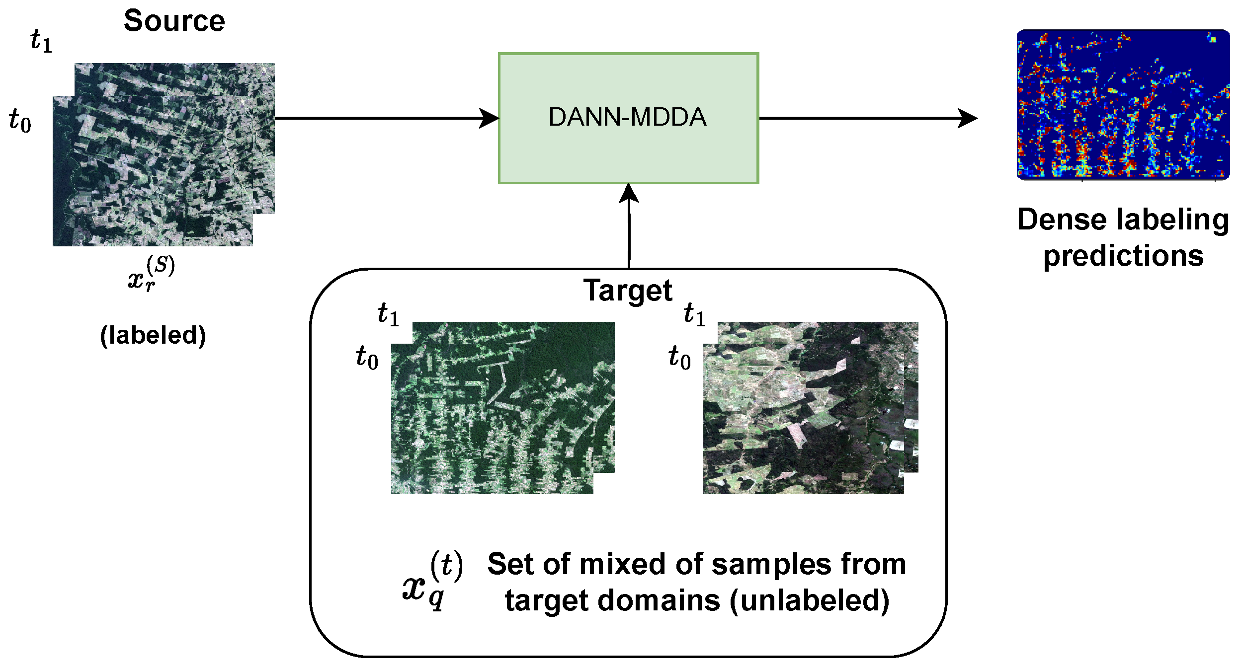
Figure 3.
Multi-Source setting.
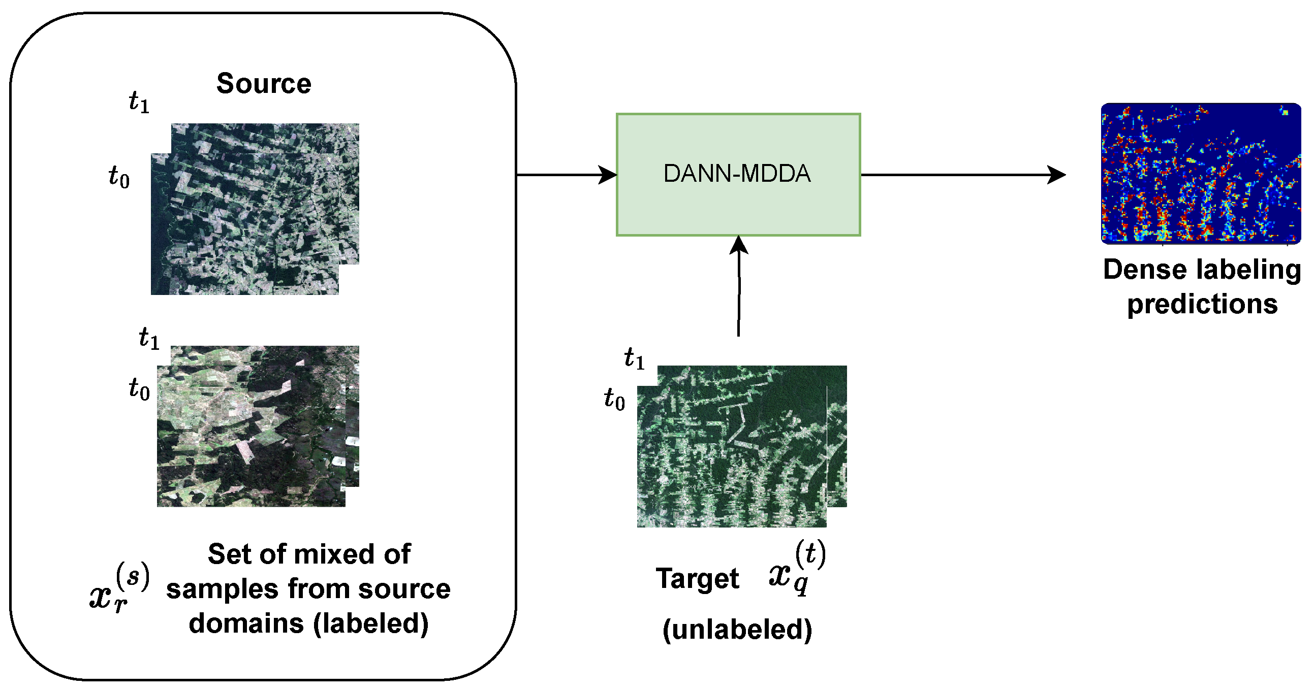
Figure 5.
Origin regions of the provided images. Adapted from [13].
Figure 5.
Origin regions of the provided images. Adapted from [13].
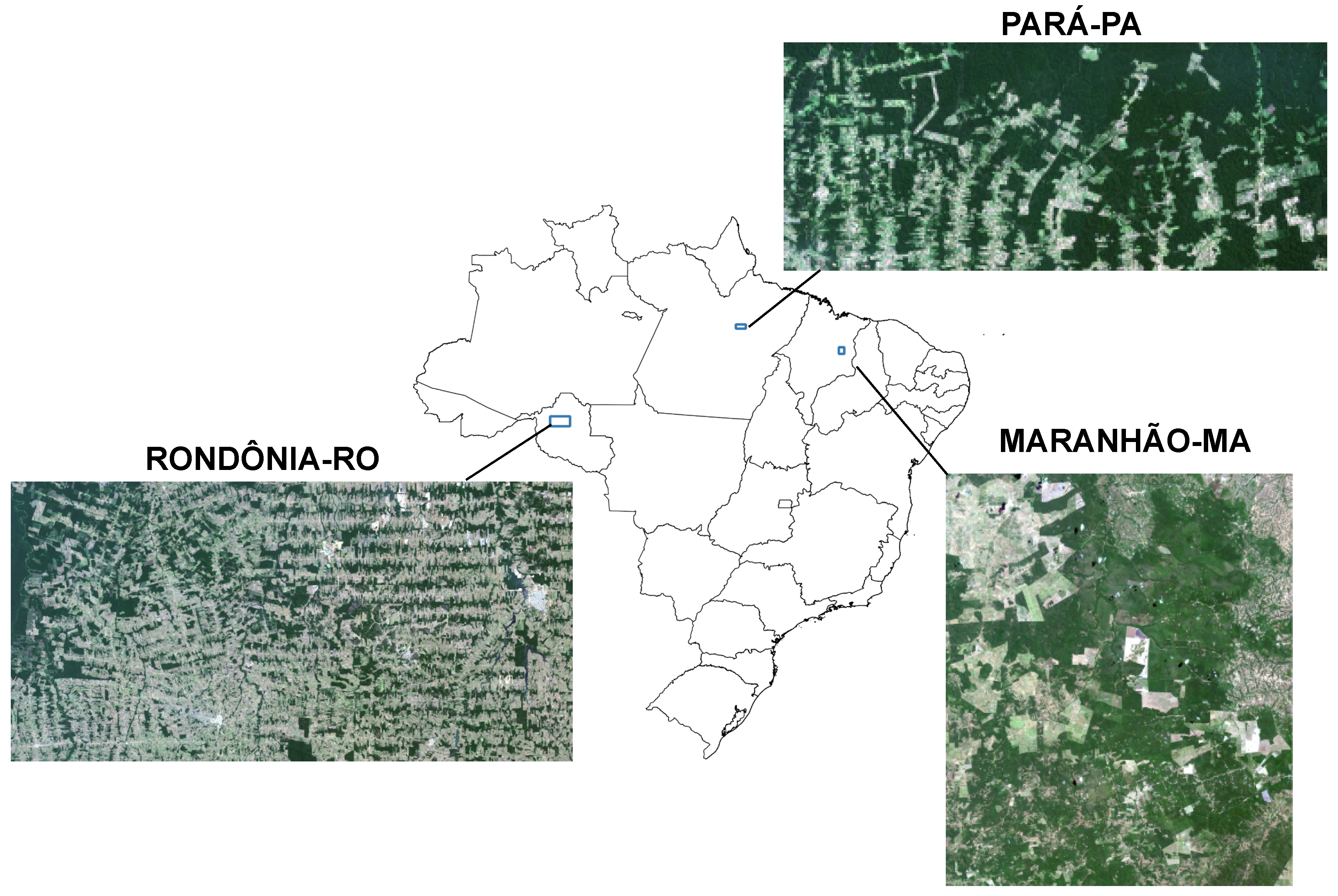
Figure 6.
Distribution of image tiles for training, validation and testing in the study areas. Adapted from [24].
Figure 6.
Distribution of image tiles for training, validation and testing in the study areas. Adapted from [24].
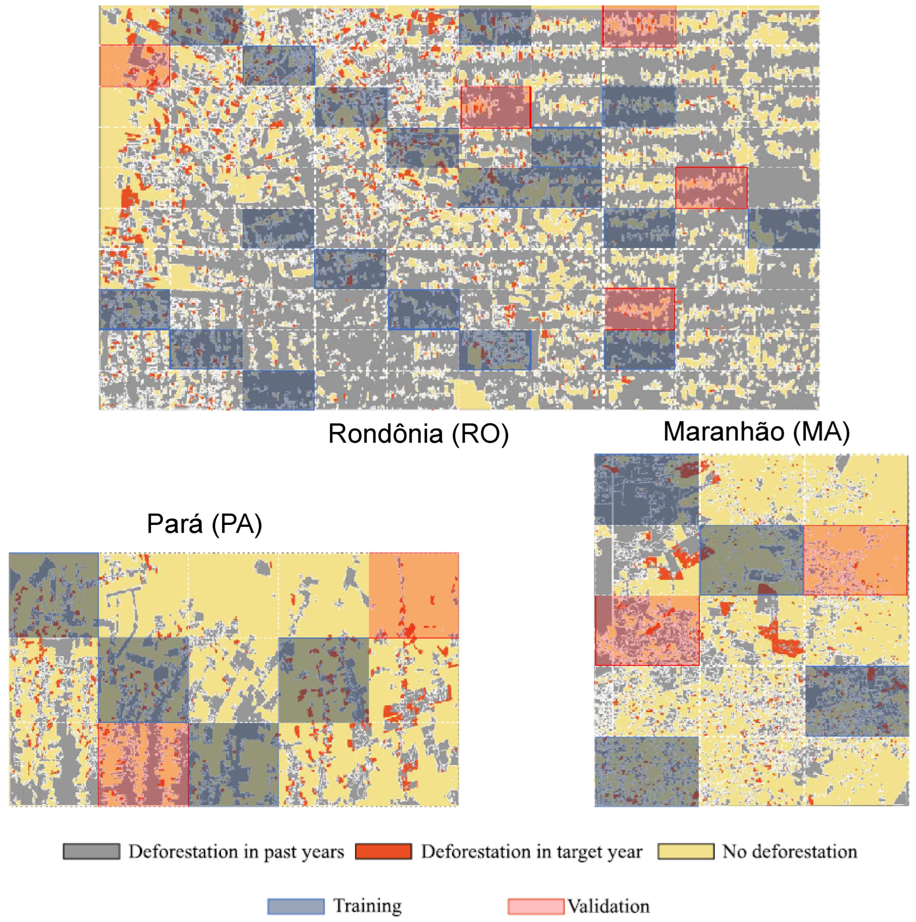
Figure 7.
Evaluation of Multi-Domain Experiments - Target MA
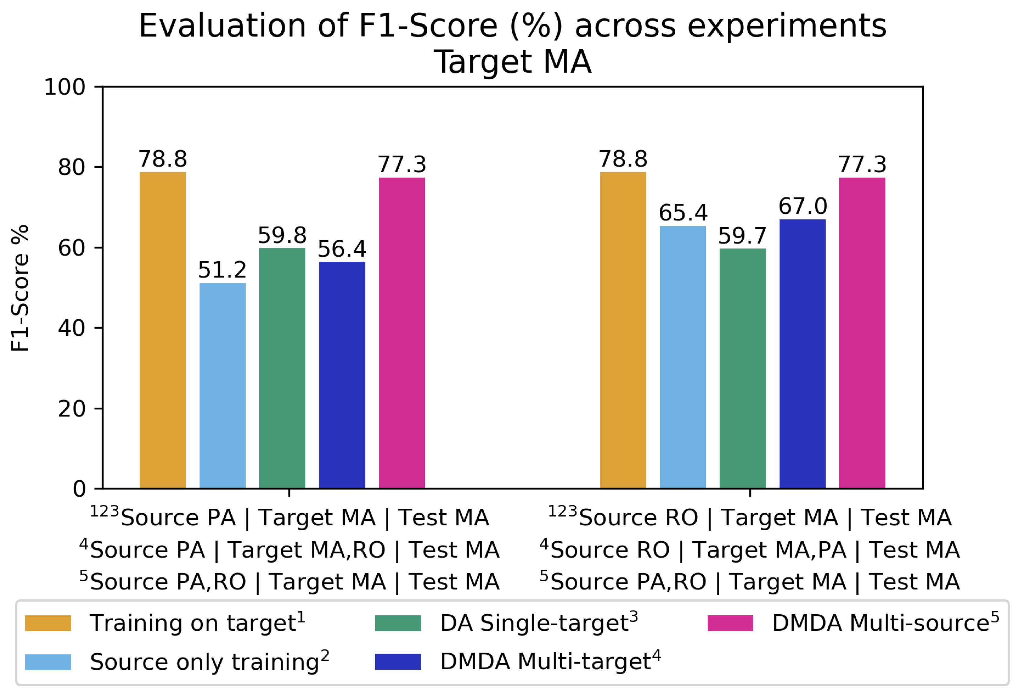
Figure 8.
Evaluation of Multi-Domain Experiments - Target PA
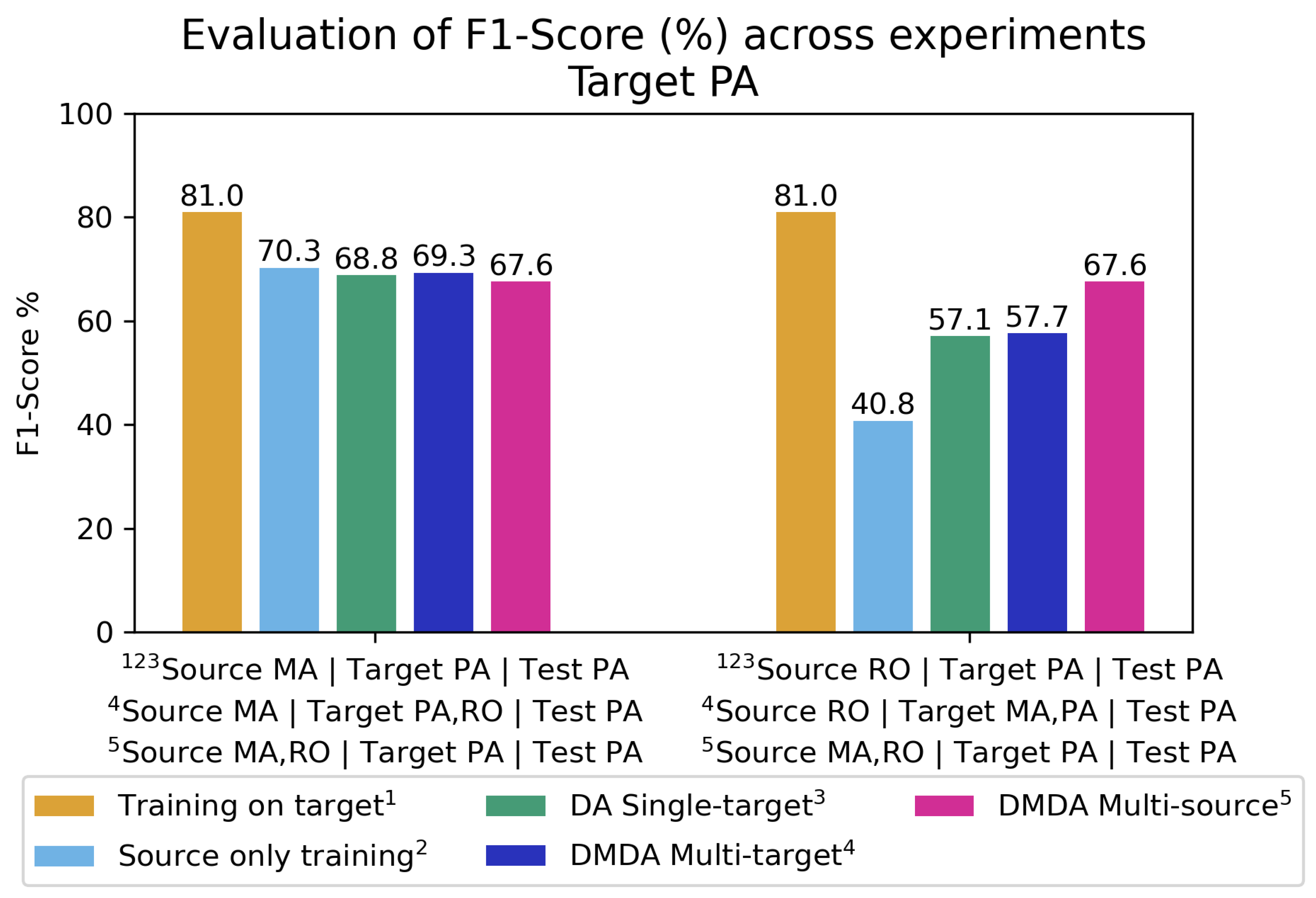
Figure 9.
Evaluation of Multi-Domain Experiments - Target RO

Table 1.
Information of each domain: image acquisition dates, classes distribution and vegetation typology.
Table 1.
Information of each domain: image acquisition dates, classes distribution and vegetation typology.
| Domains | RO | PA | MA |
|---|---|---|---|
| Vegetation | Open Ombrophilous | Dense Ombrophilous | Seasonal Deciduous and Semi-Deciduous |
| Date 1 | July 18, 2016 | August 2, 2016 | August 18, 2017 |
| Date 2 | July 21, 2017 | July 20, 2017 | August 21, 2018 |
| Deforested pixels | 225 635 (2%) | 82 970 (3%) | 71 265 (3%) |
| No-deforested pixels | 3 816 981 (29%) | 1 867 929 (65%) | 1 389 844 (57%) |
| Previously deforested pixels | 9 013 384 (69%) | 903 901 (65%) | 986 891 (40%) |
Table 2.
Additional information of each domain dataset setup.
| Domains | RO | PA | MA |
|---|---|---|---|
| Dimension (pixels) | 2550 × 5120 | 1098 × 2600 | 1700 × 1440 |
| Tiles (image subsets) | 100 | 15 | 15 |
| Tiles for Training | 2, 6, 13, 24, 28, 35, 37, 46, 47, 53, 58, 60, 64, 71, 75, 82, 86, 88, 93 | 1, 7, 9, 13 | 1, 5, 12, 13 |
| Tiles for Validation | 8, 11, 26, 49, 78 | 5, 12 | 6, 7 |
| % for Training | 20% | 26% | 26% |
| % for Validation | 5% | 13% | 13% |
| % for Testing | 75% | 60% | 60% |
Table 3.
Evaluation of mAP and F1-Score in Multi-Target Experiments. Bold values represent the highest scores, while italicized values indicate the second-highest.
Table 3.
Evaluation of mAP and F1-Score in Multi-Target Experiments. Bold values represent the highest scores, while italicized values indicate the second-highest.
| Source | MA | PA | RO | |||||||||
| Target * | PA,RO | PA,RO | MA,RO | MA,RO | MA,PA | MA,PA | ||||||
| Test | PA | RO | MA | RO | MA | PA | ||||||
| Experiments | mAP | F1 | mAP | F1 | mAP | F1 | mAP | F1 | mAP | F1 | mAP | F1 |
| Training on target | 86.4 | 81.0 | 68.3 | 68.0 | 88.4 | 78.8 | 68.3 | 68.0 | 88.4 | 78.8 | 86.4 | 81.0 |
| Source-only training | 76.8 | 70.3 | 45.7 | 47.3 | 63.3 | 51.2 | 19.9 | 20.9 | 66.9 | 65.4 | 46.0 | 40.8 |
| Single-target DA | 75.6 | 68.8 | 57.7 | 59.1 | 74.6 | 59.8 | 30.0 | 31.8 | 55.0 | 59.7 | 59.4 | 57.1 |
| DMDA Multi-target Multi-Domain Disc. |
75.3 | 69.3 | 56.5 | 58.5 | 76.2 | 56.4 | 35.4 | 36.3 | 65.7 | 67.0 | 61.2 | 57.7 |
| DMDA Multi-target Source-Target Disc. |
75.8 | 70.8 | 55.1 | 55.4 | 70.5 | 55.5 | 31.0 | 31.5 | 71.5 | 67.8 | 58.8 | 57.3 |
* Used in Multi-target experiments. In Single Target DA, the target and test domains are the same.
Table 4.
Evaluation of mAP and F1-Score in Multi-Source Experiments. Values in bold represent the highest, while values in italic indicate the second highest.
Table 4.
Evaluation of mAP and F1-Score in Multi-Source Experiments. Values in bold represent the highest, while values in italic indicate the second highest.
| Source | MA,PA | PA,RO | MA,RO | |||
| Target | RO | MA | PA | |||
| Test | RO | MA | PA | |||
| Experiments | mAP | F1 | mAP | F1 | mAP | F1 |
| Multi-source only training (No DA) | 43.2 | 44.2 | 80.7 | 77.8 | 70.3 | 62.4 |
| DMDA Multi-source Multi-Domain Disc. | 53.6 | 52.8 | 81.5 | 77.3 | 73.2 | 67.6 |
| DMDA Multi-source Source-Target Disc. | 50.6 | 53.4 | 81.1 | 77.5 | 72.0 | 67.1 |
Table 6.
F1-Score Evaluation for MA source in Multi-Target Uncertainty Estimation Experiments (AA = 3%). Values in bold represent the highest, while values in italic indicate the second highest. ’Training on target’ values are not highlighted, as they inherently represent the upper bound.
Table 6.
F1-Score Evaluation for MA source in Multi-Target Uncertainty Estimation Experiments (AA = 3%). Values in bold represent the highest, while values in italic indicate the second highest. ’Training on target’ values are not highlighted, as they inherently represent the upper bound.
| Source | MA | |||||||
| Target * | PA,RO | PA,RO | ||||||
| Test | PA | RO | ||||||
| Experiments | ||||||||
| Training on target | 81.0 | 89.3 | 64.3 | 92.9 | 68.0 | 71.7 | 52.5 | 77.0 |
| Source only training | 70.3 | 78.0 | 48.6 | 84.3 | 47.3 | 47.8 | 45.7 | 57.9 |
| DA Single-target | 68.8 | 73.1 | 58.0 | 81.4 | 59.1 | 61.3 | 50.0 | 68.8 |
| DMDA Multi-target Multi-Domain Disc. |
69.3 | 76.6 | 48.4 | 83.3 | 58.5 | 60.5 | 50.3 | 67.9 |
| DMDA Multi-target Source-Target Disc. |
70.8 | 77.0 | 53.6 | 83.6 | 55.4 | 57.4 | 47.1 | 65.3 |
* Used in Multi-target experiments. In Single Target DA, the target and test domains are the same.
Table 7.
F1-Score Evaluation for PA source in Multi-Target Uncertainty Estimation Experiments (AA = 3%). Values in bold represent the highest, while values in italic indicate the second highest. ’Training on target’ values are not highlighted, as they inherently represent the upper bound.
Table 7.
F1-Score Evaluation for PA source in Multi-Target Uncertainty Estimation Experiments (AA = 3%). Values in bold represent the highest, while values in italic indicate the second highest. ’Training on target’ values are not highlighted, as they inherently represent the upper bound.
| Source | PA | |||||||
| Target * | MA,RO | MA,RO | ||||||
| Test | MA | RO | ||||||
| Experiments | ||||||||
| Training on target | 78.8 | 86.6 | 27.5 | 87.6 | 68.0 | 71.7 | 52.5 | 77.0 |
| Source only training | 51.2 | 56.7 | 9.0 | 57.7 | 20.9 | 19.1 | 28.9 | 30.0 |
| DA Single-target | 59.8 | 66.1 | 10.8 | 67.1 | 31.8 | 30.7 | 36.8 | 41.6 |
| DMDA Multi-target Multi-Domain Disc. |
56.4 | 63.1 | 10.7 | 64.1 | 36.3 | 36.7 | 34.3 | 45.2 |
| DMDA Multi-target Source-Target Disc. |
55.5 | 61.3 | 11.1 | 62.3 | 31.5 | 30.7 | 34.9 | 41.6 |
* Used in Multi-target experiments. In Single Target DA, the target and test domains are the same.
Table 8.
F1-Score Evaluation for RO source in Multi-Target Uncertainty Estimation Experiments (AA = 3%). Values in bold represent the highest, while values in italic indicate the second highest. ’Training on target’ values are not highlighted, as they inherently represent the upper bound.
Table 8.
F1-Score Evaluation for RO source in Multi-Target Uncertainty Estimation Experiments (AA = 3%). Values in bold represent the highest, while values in italic indicate the second highest. ’Training on target’ values are not highlighted, as they inherently represent the upper bound.
| Source | RO | |||||||
| Target * | MA,PA | MA,PA | ||||||
| Test | MA | PA | ||||||
| Experiments | ||||||||
| Training on target | 78.8 | 86.6 | 27.5 | 87.6 | 81.0 | 89.3 | 64.3 | 92.9 |
| Source only training | 65.4 | 71.7 | 41.9 | 77.0 | 40.8 | 37.6 | 48.9 | 58.1 |
| DA Single-target | 59.7 | 63.5 | 47.5 | 71.3 | 57.1 | 60.1 | 49.9 | 71.8 |
| DMDA Multi-target Multi-Domain Disc. |
67.0 | 73.2 | 50.0 | 79.9 | 57.7 | 62.2 | 46.8 | 73.2 |
| DMDA Multi-target Source-Target Disc. |
67.8 | 74.9 | 33.3 | 77.7 | 57.3 | 60.4 | 48.6 | 70.6 |
* Used in Multi-target experiments. In Single Target DA, the target and test domains are the same.
Disclaimer/Publisher’s Note: The statements, opinions and data contained in all publications are solely those of the individual author(s) and contributor(s) and not of MDPI and/or the editor(s). MDPI and/or the editor(s) disclaim responsibility for any injury to people or property resulting from any ideas, methods, instructions or products referred to in the content. |
© 2025 by the authors. Licensee MDPI, Basel, Switzerland. This article is an open access article distributed under the terms and conditions of the Creative Commons Attribution (CC BY) license (http://creativecommons.org/licenses/by/4.0/).
Copyright: This open access article is published under a Creative Commons CC BY 4.0 license, which permit the free download, distribution, and reuse, provided that the author and preprint are cited in any reuse.


