Spatiotemporal Context for Daylight Saving Time-(DST-)Safety Interactions in the Contiguous United States

1. Introduction

Motor-vehicle crashes are the number two cause of unintentional deaths in the United States [1]. The consistent annual number of fatal, motor-vehicle crashes in the United States [2] and countries such as Sweden [3] confers great interest in policy consequent to such calamitous outcomes. One policy with worldwide application [2,4] purportedly relevant to the frequency and severity of motor-vehicle crashes is daylight saving time (DST). The saving of daylight in DST represents the seasonal increase in the number of hours of daylight when the majority of people are awake [5]. The effects of DST on fatal crashes emanate from natural phenomena adverse to driver behavior. Such natural phenomena are especially problematic in the contiguous United States where seasonal variation in the number of hours of daylight relative to the clock times when the majority of people drive is inherently unsafe.

So as to reconcile unpredictability and randomness in the frequency and severity of motor vehicle crashes with causation of DST [3], the study answers a question in the literature on DST-safety interactions [4,6]. Specifically, how crash-level predictors of risk such as alcohol and/or drug impairment interact with state predictors of crash exposure such as aggregate travel demand. To do so, the analyses explicitly nest crashes within states in statistical models known to contextualize spatial and temporal heterogeneity in crash outcomes to unmask DST-safety interactions in the contiguous United States and time zones.

The outline for the study is as follows. The literature review section reviews the literature on DST safety effects. The data and methodology sections, respectively, list the variables and specify the models. The results section interprets the model estimates and the discussion section presents the model results. The conclusions section highlights the contributions and limitations of the study as well as the trajectory of ongoing research.

2. Literature Review

Little unanimity in approach and impact exists in the literature on DST-safety interactions. Such safety effects emanate from the following natural phenomena. The DST-transition effect refers to changes the phenomenon where spring (forward) and fall (back) transitions demarcate periodic changes in the frequency and severity of motor-vehicle crashes. The time-of-day effect refers to the phenomenon where DST transitions change clock time relative to sunrise and sunset. The spring (forward) transition adds one hour of light relative to clock time. The fall (back) transition subtracts one hour of light relative to clock time. After the spring transition, more light later in the day supposedly increases safety at a time of the day when trips are more numerous. After the fall transition, less light later in the day supposedly decreases safety at a time of the day when trips are more numerous. The time-zone effect refers to the phenomenon where the sun rises later in the west relative to the east of a time zone at the same clock time. At the eastern extent of a time one, more light early in the day supposedly increases safety relative to the western extent. At the western extent of a time zone, less light early in the day supposedly decreases safety relative to the eastern extent.

Table 1 [2,6,7,8,9,10] is an inexhaustive list of references from the literature on DST-safety interactions. Interestingly, most references in Table 1 analyze DST-transition effects, not time-of-day, or time zone effects. The spatial scale of the study analyses is the contiguous United States so to harmonize the results of the study with the literature the list is specific to national analyses of DST-safety interactions. Subnational analyses of DST-safety interactions in states such as Minnesota [11] or New Mexico [12] are not on the list and national analyses of DST-safety interactions in countries such as Great Britain [13,14] are not on the list. See Carey and Sarma [15] for a review of an exhaustive list of references from the literature on DST-safety interactions. See Aries and Newsham [4] for a review of an exhaustive list of references from the literature on DST-energy interactions.

A critical review of the literature on DST-safety interactions specific to the contiguous United States reveals DST increases and decreases fatalities. Meyerhoff [7] reports a net decrease of −0.70% in motor-vehicle crash fatalities in March and April of 1974 with DST versus in March and April of 1973 without DST. Ferguson et al. [8] estimate about 901 fewer fatal crashes in the contiguous United States from 1987 to 1991 if DST is permanent. Varughese and Allen [9] report a statistically significant increase in fatal crashes on the Monday immediately after the spring transition and a statistically significant increase in fatal crashes on the Sunday of the fall transition. Sood and Ghosh [10] explore short- versus long-run effects of spring transitions on fatal crashes. Analysis of an experimental subsample of fatal crashes before spring transitions versus a control subsample of fatal crashes after spring transitions reveals the following. Fatal pedestrian crashes decrease from −8.00% to −11.00% in the long run after spring transitions. Fatal vehicular crashes decrease from −6.00% to −10.00% in the long run after spring transitions. The short-run effect of spring transitions on fatal crashes is not statistically significant. Smith [2] reports fatal crashes increase from +5.00% to +6.50% immediately after the spring transition in the contiguous United States from 2002 to 2011. Smith [2] also reports the spring transition causes more than thirty deaths annually at an annual social cost from $120 to $300 million. Fritz et al. [6] report fatal, motor-vehicle crash risk increases by about +6.00% in the week of the spring transition (Monday to Friday) in the contiguous United States from 1996 to 2017. The risk increase is greatest from 0400 to 0800 in the week of the spring transition (Monday to Friday) and the risk increases by +4.00% per five-degree change in longitude from east to west within a time zone in the week of the spring transition (Monday to Friday). Carey and Sarma [15] review twenty-four references to explore how implementation of a transition to Central European Time (CET) affects safety. The short-run effects of DST transitions are about zero regardless of time of day or day of week. DST transitions also seem to mitigate crashes in the long run, but confounding biases cloud interpretation of such a result.

The limitations of the Fritz et al. [6] study serve as the impetus for the present study. Specifically, the analyses include information on the number of persons in the crash police report alcohol and drug involvement. The inclusion of such information is important because alcohol and drugs are prevalent in injurious and fatal crashes [16]. The analyses also include information on the light and atmospheric conditions at the time of the crash. The inclusion of such information is important because natural phenomena such as dark-light (sunrise) and light-dark (sunset) transitions [8] and adverse weather [3] are unsafe. Finally, the analyses include information on spatial and temporal heterogeneity in the crash-level data attributable to differences from state to state in crash exposure (aggregate travel demand, licensed drivers, motor-vehicle crash fatalities, and registered vehicles).

The following sections present the data and methodology, respectively.

3. Data

Table 2 is a data dictionary for (dependent and independent) variables at the crash level as well as (independent) variables at the state level. Data for crashes are from the Fatality Analysis Reporting System (FARS) [17]. FARS is a national census of crashes in the United States. The spatial context for crashes is the states in the contiguous United States––forty-eight states plus one state equivalent (District of Columbia). Crash locations in the states are the Global Position System (GPS) coordinates (latitude, longitude) in decimal degrees. Data excludes crashes in special jurisdictions such as national park service, military, Indian reservation, college/university campus, other federal property, other, or unknown. Data also excludes crashes where GPS coordinates are not reported, not available (if state exempt), unknown, or reported as unknown. The temporal context for crashes is from January 1, 2001 to December 31, 2020. Four county/county equivalents divide time zones so data excludes the following county/county equivalents: Gulf County, Florida; Idaho County, Idaho; Malheur County, Oregon; and Stanley County, South Dakota. Fourteen county/county equivalents change time zones from 2001 to 2020 so data excludes the following county/county equivalents: Daviess, Dubois, Knox, Martin, Perry, Pike, Pulaski, and Starke in Indiana; Mercer, Morton, and Sioux in North Dakota; as well as Jones, Mellette, and Todd in South Dakota.

Dependent variables at the crash level (n = 638,164) are number of fatalities and natural log of number of fatalities [17]. Independent variables at the crash level (n = 638,164) are:

• number of persons police report alcohol involvement;
• DST (yes = 1, no = 0);
• number of persons police report drug involvement;
• latitude in decimal degrees;
• light (dawn or dusk = 1, 0 otherwise);
• longitude in decimal degrees;
• number of persons;
• number of vehicles;
• weather (adverse = 1, 0 otherwise); and
• time zone [17].

Independent variables at the state level (n = 49) are mean:

• kilometers of travel;
• number of licensed drivers;
• number of motor-vehicle crash fatalities;
• lane-kilometers of road;
• percentage of poor-quality road surfaces; and
• number of registered vehicles from 2001 to 2020 [18].

4. Methodology

Adoption of a multilevel approach contextualizes DST-safety interactions. Advantages of such an approach are twofold. First, multilevel models explicitly nest crashes within states. Second, two sets of parameters summarize average relationships as well as variation in average relationships between crashes and independent variables hypothesized to interact with crashes.

Multilevel models in the analyses are two-level models of crashes (c) at the micro-level nested within states (s) at the macro-level [19]. Number of fatalities or natural log of number of fatalities are a function of crash-level independent variables plus a crash-level error term:

Y_cs = β_0s + β_1sX_1cs + β_2sX_2cs + … + β_PsX_Pcs + r_cs,

(1)

where

• Y_cs is number of fatalities or natural log of number of fatalities in crash c in state s;
• β_Ps are (p = 0, 1, 2, …, P) crash-level coefficients;
• X_Pcs is crash-level predictor P for crash c in state s;
• r_cs is the crash-level error term; and
• σ² is the variance of crash-level error term r_cs.

The model for variation in number of fatalities or natural log of number of fatalities between states is as follows:

β_0s = γ₀₀ + γ₀₁W_1s + γ₀₂W_2s + γ_0QW_Qs + … + μ_0s,

(2)

where

• γ₀₀ is the y-intercept term for crash effect β_0s;
• γ_0Q are (q = 1, 2, …, Q) state-level coefficients;
• W_Qs is state-level predictor Q in state s;
• u_0s is the state-level error term; and
• τ₀₀ is the variance of state-level error term u_0s.

y-intercepts and coefficients at the first level of two-level models are fixed or random. y-intercepts are random at the first level of random-intercept models in the analyses. y-intercepts as well as latitude and longitude coefficients are random at the first level of random-coefficients models in the analyses.

5. Analysis

Before presenting analyses results, statistical problems with model specification are noteworthy. Failure of full models of state-level independent variables to converge points to problems with the fixed portions of models. Unsurprisingly, a Pearson correlation coefficient matrix shows multicollinearity is evident amongst the macro-level predictors. Analyses that complete without errors and yield interpretable estimates are models with licensed drivers as the macro-level predictor. Such a result is consistent with results from the Pearson correlation coefficient matrix where coefficients for licensed drivers are statistically significant at the 10.00% confidence level, but less than |0.50| in magnitude. The following subsections, therefore, present random-intercept and -coefficients model results, respectively, with licensed drivers at the state level.

5.1. Contiguous United States

Descriptive statistics for crashes and states in the contiguous United States are in Table 3. The following subsections present the random-intercept and -coefficients model results, respectively, for the contiguous United States.

5.1.1. Random-Intercept Model Results for Contiguous United States

Estimates from random-intercept models for the contiguous United States are in Table 4. The left column (Fatalities) presents estimates for number of fatalities. The right column (lnFatalities) presents estimates for natural log of number of fatalities. Consistent with expectations [12], fatalities increase (by +1.00%) as alcohol involvement increases. Surprisingly, fatalities decrease slightly (by −0.10%) if the crash is in DST. Consistent with results for alcohol, fatalities increase (by +2.00%) as drug involvement increases. Surprisingly, fatalities increase slightly (by +0.10%) as latitude increases from south to north. Fatalities increase slightly (by +0.30%) if the crash is at dawn or dusk [20]. Consistent with the time-zone safety effect [6], fatalities decrease slightly (by −0.10%) as longitude increases from west to east. Consistent with expectations, fatalities increase (by +4.00%) as persons increases. Surprisingly, fatalities decrease (by −2.00%) as vehicles increases. Fatalities decrease from the Mountain to Eastern time zone (by −2.00%) and the Pacific to Eastern time zone (by −3.00%).

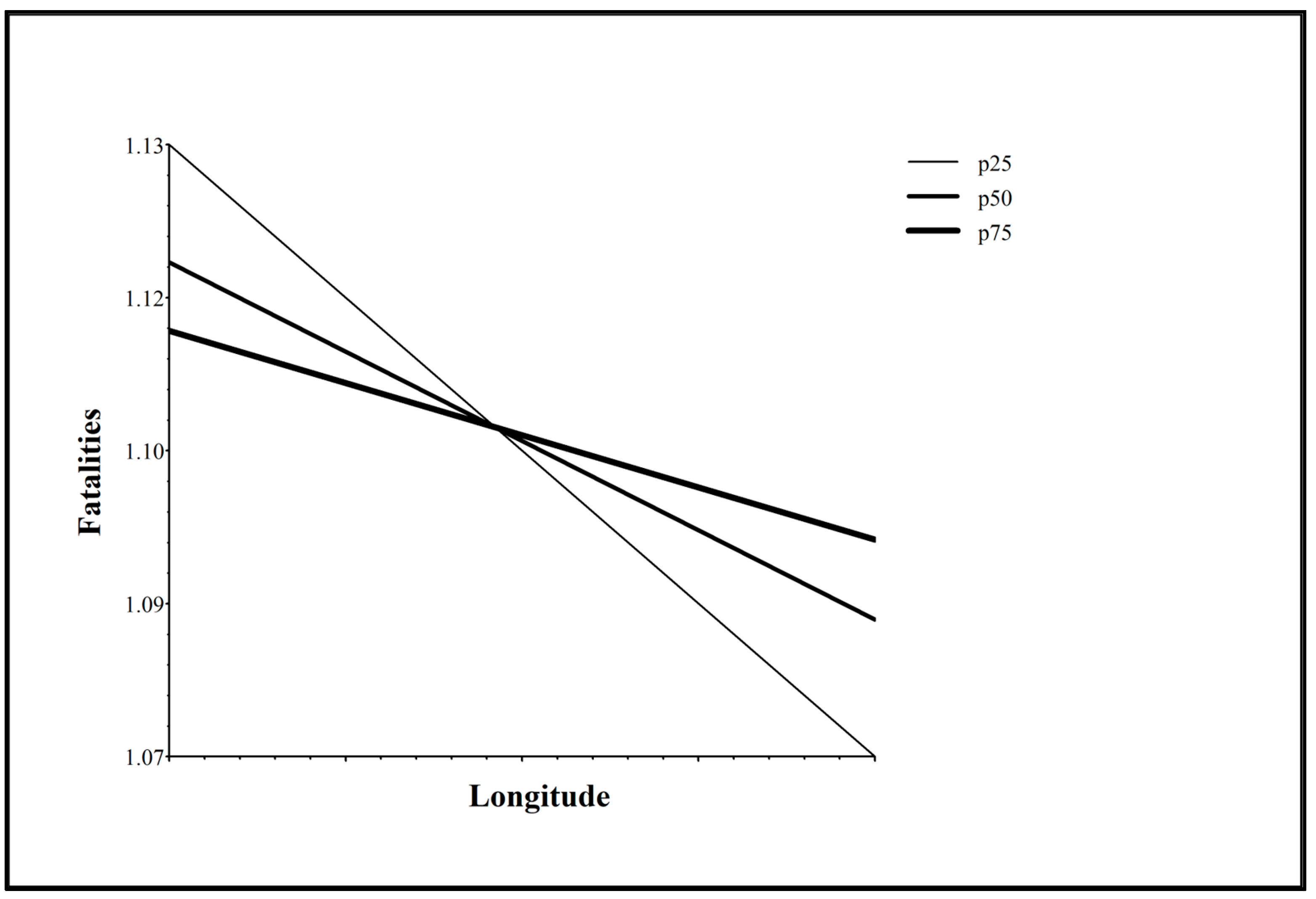
5.1.2. Random-Coefficients Model Results for Contiguous United States

Estimates from random-coefficients models for the contiguous United States are in Table 5. The left column (Fatalities) presents estimates for number of fatalities. The right column (lnFatalities) presents estimates for natural log of number of fatalities. The effects of licensed drivers on latitude and longitude are statistically significant. With regard to the former, the effect of licensed drivers on fatalities decreases very slightly (by +0.001%) as latitude increases from south to north. With regard to the latter, the effect of licensed drivers on fatalities increases very slightly (by +0.001%) as longitude increases from west to east.

Figure 1 shows how the licensed-drivers effect on fatalities changes by longitude in the contiguous United States. The negative slopes for the 25th (p25), 50th (p50), and 75th percentiles (p75) show fatalities decrease from west to east. At the western extent of the contiguous United States, fatalities are highest in states where licensed drivers are less numerous such as in California. At the eastern extent of the contiguous United States, fatalities are highest in states where licensed drivers are more numerous such as in Vermont. The point of intersection of the negative slopes for p25, p50, and p75 in Figure 1 represents the longitude where the licensed-drivers effect is null in the contiguous United States. Figure 2 is a choropleth map of licensed drivers in the contiguous United States. Manual classification represents the following four classes: less than 25th Percentile (p25); 25th Percentile (p25) to 49th Percentile (p49); 50th Percentile (p50) to 74th Percentile (p74); and greater than or equal to 75th Percentile (p75) of licensed drivers. Class breaks represent p25, p50, and p75 of the licensed-drivers distribution. The graticule of longitudes in Figure 2 shows the following states (from north to south) represent the geographic location from about −100 to −95 where the licensed-drivers effect is null in the contiguous United States: North Dakota; Minnesota; South Dakota; Iowa; Nebraska; Missouri; Kansas; Oklahoma; and Texas.

5.2. Time Zones

The highest levels of aggregation are the most sensitive to sample size thresholds for accurate parameter and error estimates in full, multilevel models [21]. Since the respective sample sizes for states in the Pacific and Mountain time zones are not sufficient, the results below are for the Pacific plus Mountain, Central, and Eastern time zones, respectively.

Descriptive statistics for crashes and states in the Pacific plus Mountain, Central, and Eastern time zones are in Table 6. The following subsections present the random intercept and -coefficients model results, respectively, for the Pacific plus Mountain, Central, and Eastern time zones.

5.2.1. Random-Intercept Model Results for Time Zones

Estimates from random-intercept models for time zones are in Table 7. The left columns (Fatalities) present estimates for number of fatalities. The right columns (lnFatalities) present estimates for natural log of number of fatalities. Consistent with expectations [12], fatalities increase as alcohol involvement increases in the Pacific plus Mountain (by +1.00%), Central (by +1.00%), and Eastern time zones (by +1.00%). Interestingly, fatalities increase slightly if the crash is in DST in the Pacific plus Mountain time zone (by +0.30%), but decrease slightly if the crash is in DST in the Central (by −0.30%) or Eastern time zones (by −0.20%). Consistent with results for alcohol, fatalities increase as drug involvement increases in the Pacific plus Mountain (by +2.00%), Central (by +2.00%), and Eastern time zones (by +2.00%). Fatalities increase slightly as latitude increases from south to north in the Pacific plus Mountain (by +0.30%) and Eastern time zones (by +0.10%), but not the Central time zone. Interestingly, fatalities increase if the crash is at dawn or dusk in the Central time zone (by +1.00%), but not the Pacific plus Mountain or Eastern time zones. Fatalities increase slightly as longitude increases from west to east in the Pacific plus Mountain time zone (by +0.20%), but decrease slightly as longitude increases from west to east in the Central (by −0.20%) and Eastern time zones (by −0.10%). Consistent with expectations, fatalities increase as persons increase in the Pacific plus Mountain (by +4.00%), Central (by +4.00%), and Eastern time zones (by +3.00%). Surprisingly, fatalities decrease as vehicles increases in the Pacific plus Mountain (by −2.00%), Central (by −1.00%), and Eastern time zones (by −2.00%). Fatalities decrease very slightly as licensed drivers increase in the Pacific plus Mountain time zone (by −0.02%), but increase very slightly as licensed drivers increase in the Eastern time zone (by +0.01%).

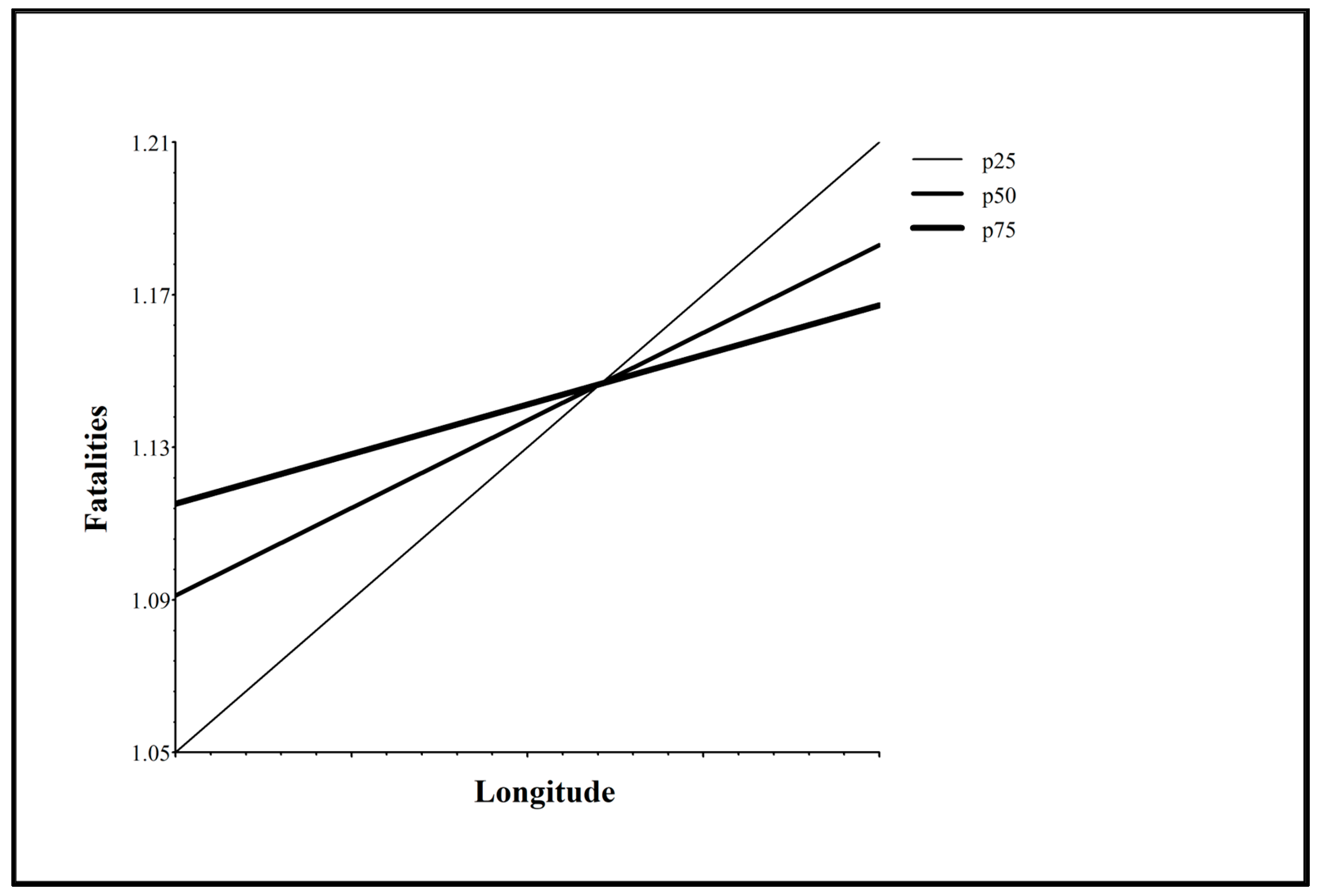
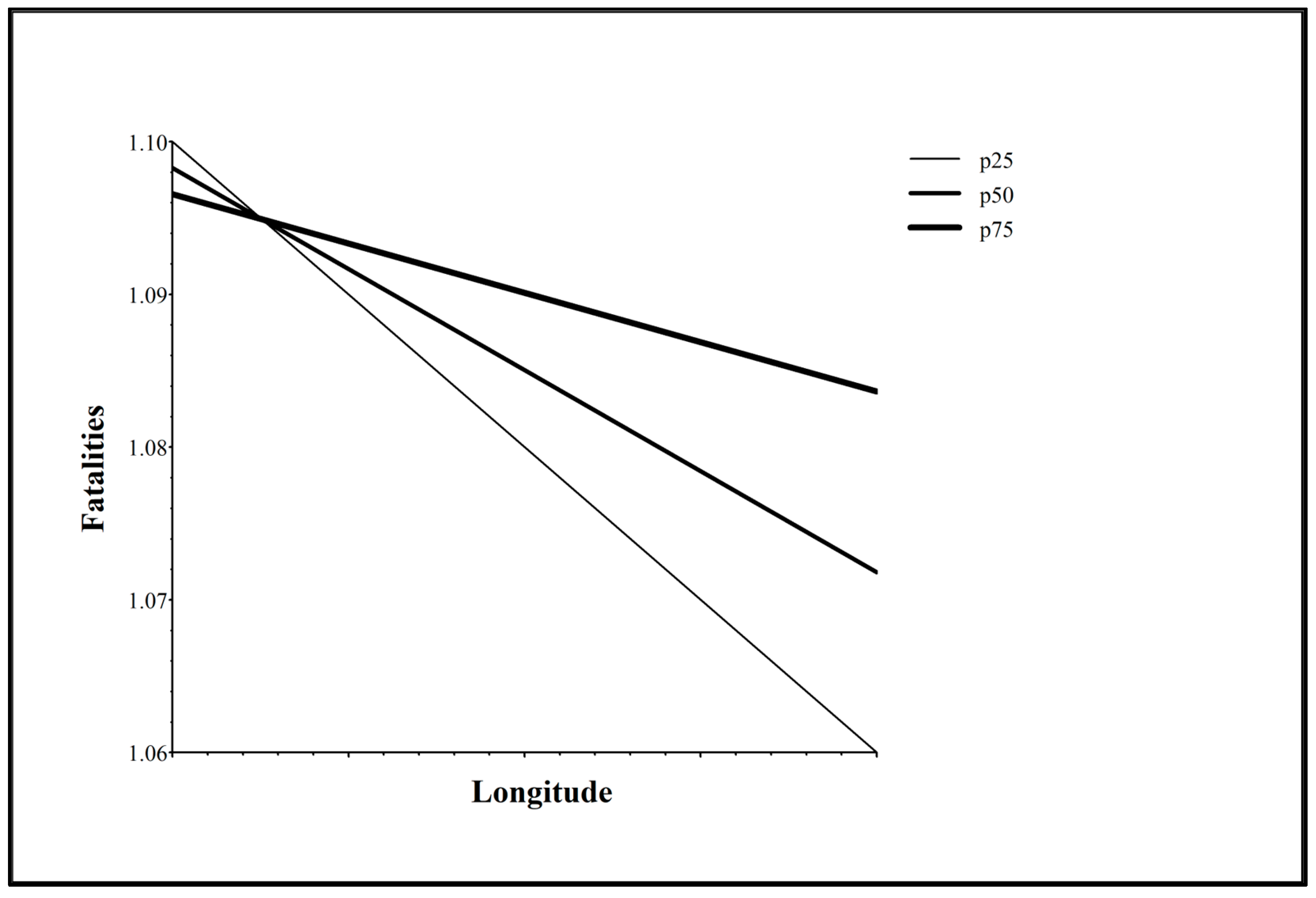
5.2.2. Random-Coefficients Model Results for Time Zones

Estimates from random-coefficients models for time zones are in Table 8. The left columns (Fatalities) present estimates for number of fatalities. The right columns (lnFatalities) present estimates for natural log of number of fatalities. The effects of licensed drivers on latitude and longitude are statistically significant in the Pacific plus Mountain and Eastern time zones, but not the Central time zone. With regard to the former, the effect of licensed drivers on fatalities decreases very slightly as latitude increases from south to north in the Pacific plus Mountain (by −0.01%) and Eastern time zones (by −0.002%). The effect of licensed drivers on fatalities changes from Pacific plus Mountain to Eastern time zones as longitude increases from west to east. The licensed drivers effect on fatalities decreases very slightly as longitude increases from west to east in the Pacific plus Mountain time zone (by −0.01%), but increases very slightly as longitude increases from west to east in the Eastern time zone (by +0.001%).

Figure 3 shows how the licensed-drivers effect on fatalities changes by longitude in the Pacific plus Mountain time zone. The positive slopes for p25, p50, and p75 show fatalities increase from west to east in the Pacific plus Mountain time zone. At the western extent of the Pacific plus Mountain time zone, fatalities are highest in states where licensed drivers are more numerous such as in Washington. At the eastern extent of the Pacific plus Mountain time zone, fatalities are highest in states where licensed drivers are less numerous such as in New Mexico. The point of intersection of the positive slopes for p25, p50, and p75 in Figure 3 represents the longitude where the licensed-drivers effect is null in the Pacific plus Mountain time zone.

Figure 4 shows how the licensed-drivers effect on fatalities changes by longitude in the Eastern time zone. The negative slopes for p25, p50, and p75 show fatalities decrease from west to east in the Eastern time zone. At the western extent of the Eastern time zone, fatalities are highest in states where licensed drivers are less numerous such as in Kentucky. At the eastern extent of the Eastern time zone, fatalities are highest in states where licensed drivers are more numerous such as in Vermont. The point of intersection of the negative slopes for p25, p50, and p75 in Figure 4 represents the longitude where the licensed-drivers effect is null in the Eastern time zone.

6. Discussion

Contiguous United States as well as (Pacific plus Mountain, Central, and Eastern) time zone analyses of DST-safety interactions reveal the following. The slight decrease in fatalities during DST in the contiguous United States masks an increase in fatalities during DST in the Pacific plus Mountain time zone. The slight increase in fatalities during sunrise or sunset in the contiguous United States is representative of the increase in fatalities during sunrise and sunset in the Central time zone, not the Pacific plus Mountain or Eastern time zones. The latter result is probably because of changes in relief from the Pacific plus Mountain to the Central to the Eastern time zones (Figure 5). The slight increase in fatalities as latitude increases from south to north in the contiguous United States is representative of the slight increase in fatalities as latitude increases from south to north in the Pacific plus Mountain and Eastern time zones, not the Central time zone. The latter result is probably because the clock times of sunrise and sunset vary more from season to season at the northern extent of latitude in the contiguous United States at +49 than at the southern extent of latitude in the contiguous United States at +25 [5]. For example, at +49 the clock time of sunrise ranges from about 0800 in January to about 0400 in June, but at +25 the clock time of sunrise ranges from about 0700 in January to about 0500 in June. And, at +49 the clock time of sunset ranges from about 0400 in January to about 0800 in June, but at +25 the clock time of sunset ranges from about 0500 in January to about 0700 in June. The time zone-effect in the contiguous United States where fatalities increase from east to west (Figure 1) masks offsetting effects from the Pacific plus Mountain time zone where fatalities decrease from east to west (Figure 3) to the Eastern time zone where fatalities increase from east to west (Figure 4). Interestingly, the magnitudes of the time zone-effects in the study are far lower than the magnitude of the time zone effect in the literature of +4.00% per five-degree change in longitude from east to west in a time zone [6]. The magnitudes in the study are probably far lower because of differences in measures of crash severity and temporal units of analysis. The measure of crash severity in the study is number of fatalities versus incidence rate ratio in Fritz et al. [6] and the temporal unit of analysis in the study is the year versus the week in Fritz et al. [6].

To return to the statistical problems with model specification, on the one hand, failure of full models of state-level independent variables to converge suggests that crash exposure in terms of aggregate travel demand, motor-vehicle crash fatalities, and registered vehicles are endogenous to DST-safety interactions. The latter result is inconsistent with the literature on the effect of traffic volumes on fatal crashes [3]. The result in the study is probably inconsistent because of differences in measurement and methodology. The study uses aggregate travel demand to measure traffic volumes while Fridstrøm, et al. [3] use traffic counts to measure traffic volumes in Denmark and gasoline sales to approximate traffic volumes in Finland, Norway, and Sweden. The similarity of sources for the forty-eight states plus the one state equivalent (District of Columbia) in the study creates one database amenable to exploration of both within- and between state, spatial and temporal variation. The dissimilarity of sources for the four countries in Fridstrøm, et al. [3] creates four databases amenable to exploration of only within country, spatial and temporal variation. Therefore, the effect of traffic volumes on fatal crashes is fixed from country to country in Fridstrøm, et al. [3] which is theoretically and empirically implausible.

On the other hand, the fact that models with information on differences from state to state in crash exposure in terms of licensed drivers successfully converge is worthy of discussion. Clearly, crash exposure in terms of licensed drivers effectively, if not modestly, explains spatial heterogeneity in the crash-level data. Policy implications for state government to intervene on crash exposure in terms of licensed drivers are as follows [16]. First, since state governments regulate operator licensure not the federal government, limit or eliminate the crash exposure of drivers whose records of impairment due to alcohol and/or drugs are known to law enforcement via temporary or permanent licensure forfeiture. Second, interdiction by law enforcement where impairment from alcohol and/or drugs amongst drivers is prevalent both within and between states.

7. Conclusions

The most important contributions of the study derive from measurement and methodological advancements to the literature on DST-safety interactions. Twenty years (from 2001 to 2020) of fatal crashes in the forty-eight states plus the one state equivalent in the contiguous United States approximate the temporal and spatial extent representative of the literature on DST-safety interactions. Adoption of a multilevel approach unmasks differences in DST-safety interactions both within and between time zones. The subsequent analyses answer a call [6] in the literature on DST-safety interactions to account for geographical differences [4] from state to state which affect the frequency and severity of motor-vehicle crashes in the context of DST-related natural phenomena. Results from multilevel models of fatal crashes which account for geographical differences in the contiguous United States and time zones help to contextualize DST-safety interactions which are ambiguous, at best, in the literature.

The most glaring omission is the absence of any analyses, regardless of scale, on DST-transition safety effects. Specifically, a multilevel approach which nests crashes within the hours, days, or weeks before and after DST transitions, both spring and fall, within states may help to contextualize the DST-transition safety effect in a new, empirically-justified model. Given the many past efforts to understand how DST transitions affect safety, the topic is ideally suitable for the next iteration of research on the general topic of DST-safety interactions.

References

1. Centers of Disease Control and Prevention. Top Ten Leading Causes of Death in the U.S. for Age 1-44 from 1981-2023. 2025. Available online: https://wisqars.cdc.gov/animated-leading-causes/ (accessed on 10 March 2025).
2. Smith, A. Spring forward at your own risk: daylight saving time and fatal vehicle crashes. Am. Econ. J.: Appl. Econ. 2016, 8, 65–91. [Google Scholar] [CrossRef]
3. Fridstrøm, L.; Ifver, J.; Ingebrigsten, S.; Kulmala, R.; Thomsen, L. Measuring the contribution of randomness, exposure, weather, and daylight to the variation in road accident counts. Accident Anal. Prev. 1995, 27, 1–20. [Google Scholar] [CrossRef] [PubMed]
4. Aries, M.; Newsham, G. Effect of daylight saving time on lighting energy use: a literature review. Energ. Policy 2008, 36, 1858–1866. [Google Scholar] [CrossRef]
5. Bartky, I.; Harrison, E. Standard and daylight-saving time. Sci. Am. 1979, 240, 46–53. [Google Scholar] [CrossRef]
6. Fritz, J.; VoPham, T.; Wright, K.; Vetter, C. A chronobiological evaluation of the acute effects of daylight saving time on traffic accident risk. Curr. Biol. 2020, 30, 729–735.e2. [Google Scholar] [CrossRef] [PubMed]
7. Meyerhoff, N. The influence of daylight saving time on motor vehicle fatal traffic accidents. Accident Anal. Prev. 1978, 10, 207–221. [Google Scholar] [CrossRef]
8. Ferguson, S.; Preusser, D.; Lund, A.; Zador, P.; Ulmer, R. Daylight saving time and motor vehicle crashes: the reduction in pedestrian and vehicle occupant fatalities. Am. J. Public Health 1995, 85, 92–95. [Google Scholar] [CrossRef] [PubMed]
9. Varughese, J.; Allen, R. Fatal accidents following changes in daylight savings time: the American experience. Sleep Med. 2001, 2, 31–36. [Google Scholar] [CrossRef] [PubMed]
10. Sood, N.; Ghosh, A. The short and long run effects of daylight saving time on fatal automobile crashes. The B.E. J. Econ. Anal. Poli. 2007, 7, 11. [Google Scholar] [CrossRef]
11. Huang, A.; Levinson, D. The effects of daylight saving time on vehicle crashes in Minnesota. J. Safety Res. 2010, 41, 513–520. [Google Scholar] [CrossRef] [PubMed]
12. Hicks, G.; Davis, J.; Hicks, R. Fatal alcohol-related traffic crashes increase subsequent to changes to and from daylight savings time. Percept. Motor Skill. 1998, 86, 879–882. [Google Scholar] [CrossRef] [PubMed]
13. Broughton, J.; Hazelton, M.; Stone, M. Influence of light level on the incidence of road casualties and the predicted effect of changing ‘summertime’. J. R. Statist. Soc. A 1999, 162, 137–175. [Google Scholar] [CrossRef]
14. Singh, R.; Sood, R.; Graham, D. Road traffic casualties in Great Britain at daylight savings time transitions: a casual regression discontinuity design analysis. BMJ Open 2022, 12, e054678. [Google Scholar] [CrossRef] [PubMed]
15. Carey, R.; Sarma, K. Impact of daylight saving time on road traffic collision risk: A systematic review. BMJ Open 2017, 7, e014319. [Google Scholar] [CrossRef] [PubMed]
16. Thomas, F.; Darrah, J.; Graham, L.; Berning, A.; Blomberg, R.; Finstad, K.; Griggs, C.; Crandall; Schulman, C.; Kozar, R.; Lai, J.; Mohr, N.; Chenoweth, J.; Cunningham, K.; Babu, K.; Dorfman, J.; Van Heukelom, J.; Ehsani, J.; Fell, J.; Whitehill, J.; Brown, T.; Moore, C. Alcohol and Drug Prevalence Among Seriously or Fatally Injured Road Users. 2022. Available online: https://www.nhtsa.gov/sites/nhtsa.gov/files/2022-12/Alcohol-Drug-Prevalence-Among-Road-Users-Report_112922-tag.pdf (accessed on 10 March 2025).
17. United States Department of Transportation. (2022a). Fatality Analysis Reporting System (FARS). Available online: https://www.nhtsa.gov/research-data/fatality-analysis-reporting-system-fars (accessed on 10 March 2025).
18. United States Department of Transportation. Highway Statistics. 2022b. Available online: https://www.fhwa.dot.gov/policyinformation/statistics.cfm (accessed on 10 March 2025).
19. Raudenbush, S.; Bryk, A. Hierarchical Linear Models: Applications and Data Analysis Methods. Sage: Thousand Oaks, CA, USA, 2002.
20. Monk, T. Traffic accident increases as a possible indicant of desynchronosis. Chronobiologia 1980, 7, 527–529. [Google Scholar] [PubMed]
21. Maas, C.; Hox, J. Sufficient sample sizes for multilevel modeling. Methods. 2005, 1, 86–92. [Google Scholar] [CrossRef]
22. United States Geological Survey. The National Map - Data Delivery. 2019. Available online: https://www.usgs.gov/NationalMap/data (accessed on 10 March 2025).
Disclaimer/Publisher’s Note: The statements, opinions, and data contained in all publications are solely those of the individual author(s) and contributor(s) and not of MDPI and/or the editor(s). MDPI and/or the editor(s) disclaim responsibility for any injury to people or property resulting from any ideas, methods, instructions, or products referred to in the content.
Figure 1. Changes in licensed-drivers effect on fatalities by longitude in the contiguous United States.
Preprints 152184 g001
Figure 2. Choropleth map of licensed drivers in the contiguous United States.
Preprints 152184 g002
Figure 3. Changes in licensed-drivers effect on fatalities by longitude in the Pacific plus Mountain time zones.
Preprints 152184 g003
Figure 4. Changes in licensed-drivers effect on fatalities by longitude in the Eastern time zones.
Preprints 152184 g004
Figure 5. Elevation profile from west (Los Angeles) to east (New York City) coasts of contiguous United States (X = Mississippi River) [22].
Preprints 152184 g005