
Submitted:
17 March 2025
Posted:
18 March 2025
You are already at the latest version
Abstract
Air temperatures are rising rapidly, and January 2025 was recorded as the warmest January ever, underscoring the urgent need to address increasing CO₂ levels. Carbon emissions, driven by energy-intensive household consumption, are a primary contributor to the climate crisis, making strategies for reducing emissions and transitioning to a low-carbon economy critical. Households account for a significant share of global emissions, and in Türkiye, rapid population growth and evolving consumption patterns have intensified energy demand. This study investigates two key research questions: (1) the relationship between household income distribution and the carbon footprint, and (2) how variations in consumption patterns influence the carbon footprint. Employing the PRICES microsimulation model (O’Donoghue et al., 2023), we integrate detailed expenditure data from Türkiye’s 2019 Household Budget Survey with a 2016 Input-Output table from the World Input-Output Database to simulate both direct and indirect CO₂ emissions. This study focuses on, understanding household distributional drivers of carbon emission.
Keywords:
households
; carbon emission
; distributional drivers
; microsimulation
1. Introduction
Air temperatures are rising rapidly, with increasing carbon emissions being a major cause. January 2025 was the warmest January ever recorded, according to the World Meteorological Organization, highlighting how rising CO2 levels are worsening the climate crisis. The urgent need to understand driver of carbon emissions and households play a critical role in this effort. Households account for approximately three-quarters of global carbon emissions, so household energy consumption is crucial to understanding the drivers of carbon emissions (Benders et al., 2006; Larsen and Hertwich, 2010; Zeng et al., 2021, Li et al., 2017)). In addition, middle-income countries have become major contributors of today’s new carbon emissions due to their growing economies. (World Emissions Clock, World Data Lab; Dorband, 2019; Steckel, 2012). As a result, strategies for reducing CO2 emissions and transitioning to a low-carbon economy have become key global priorities. Given concerns about the negative distributional impact of these strategies on households, it is important to understand the factors which drive these negative distributional outcomes. In this paper we develop a methodology to unpick these different drivers to understand these distributional forces in a middle-income setting.
Many of these studies have similarities in considering the distributional characteristics, both vertically and horizontally (Steckel et al., 2021) of carbon taxes and occasionally the joint impact of resulting revenue recycling (Can et al., 2025; Saelim, 2019; Renner, 2018). Even the basic science is the same, with consistent differential emissions per unit of energy, across countries, what is clear from distributional studies (Steckel et al., 2021, Linden et al. 2024; Elgouacem et al., 2024) is that there is significant cross-country heterogeneity. In this paper we explore the distributional characteristics of the underling drivers of carbon emissions and associated carbon pricing.
In order to effectively manage and reduce household-associated emissions (Xie et al., 2023) it is necessary therefore to understand these underling distributional drivers. Existing research based on survey data on household consumption expenditure has identified the key determinants of Carbon Footprints (CF) (e.g., Serino and Klasen, 2015; Druckman & Jackson, 2016, Ivanova et al., 2020). Wang et al. (2022) find (Household Carbon Footprints) HCFs are unevenly distributed because consumption patterns vary based on household characteristics and lifestyles. The carbon footprint of a region, whether a city or a country, includes emissions produced directly and indirectly throughout global supply chains to meet final consumption in that area (Matthews et al. 2008; Hertwich et al. 2009). Income is often considered the primary predictor of household carbon footprints (CF), although some studies, such as Minx et al. (2013), argue that other socio-economic characteristics can be equally important. In fact, Vita et al. (2020) found that higher income does not necessarily lead to a larger footprint, particularly among participants of environmental initiatives. This article provides a review of on the direct distributional drivers of carbon emission such as income, savings, budget shares, differential carbon emissions, prices and policy as opposed to indirect drivers such as household socio-economic characteristics. In addition instead of considering the mean impact of these drivers on emissions (Coruh et al., 2024), we consider the distributional characteristics of these drivers.
We are trying to draw a picture of the responsibility of household consumption patterns on carbon emissions with the income distribution decile. The aim of the study is to assess households on the basis of the factors that cause increased energy consumption and CO2 emissions in Türkiye and to shed light on the complex relationship between household distributional drivers of carbon emission. We consider to contribute with two dimensions. First, we explore the relationship between household income distribution and the carbon footprint. Second, we examine how variations in individual drivers of consumption patterns influence the carbon footprint.
In this paper we take as a case study a large rapidly changing middle income country, Türkiye that lies in an important geopolitical position on the border between Europe, the Middle East and Central Asia. Türkiye’s energy demand has risen sharply over the past two decades due to population growth and changing consumption trends. Energy use is essential for economic growth but also a major source of greenhouse gas emissions (Jacob et al. 2014). Households accounted for 8.8% of final energy use, while manufacturing had the largest share at 41.5%. In 2021, energy use reached 5,560 petajoules, up 9.8% from the previous year. In 2022, household energy consumption in Türkiye totalled 1.29 million terajoules, mainly from natural gas (48.3%), electricity (17.1%), and coal (14.3%) (TURKSTAT). It is in many ways typical of many middle-income countries in relation to the pressures it faces in to relation to decarbonisation. It faces a trade-off between the impact of climate change, given its geographical position, economic growth and energy security. Like many middle-income countries, difficulties in access gas during the Russian-Ukraine conflict saw the trend in relation to the reduction in coal powered electricity generation reversed.
This paper aims to provide a robust framework to discuss distributional drivers of carbon emission, taking into account the heterogeneous economic conditions of households, their wealth levels and their energy preferences, and to provide a guide for making effective policy choices. To realize this goal, we applied the PRICES microsimulation model (O’Donoghue et al., 2023). The model relies on household budget survey data, incorporating detailed spending patterns, self-consumption (where applicable), and socio-economic factors The PRICES model includes algorithms that can be adapted to different policy environments of countries, and these algorithms include comprehensive tools for assessing welfare and distributional impacts and for understanding the link between consumption behaviour and its environmental impact across different segments of the population
This article proceeds as follows: Section II outlines theoretical framework Section III explains data sources and methodology, Section presents IV the results, and Section V discusses policy implications and concludes the analysis.
2. Theoretical Framework
Human consumption activities have a permanent impact on nature. The carbon footprint is a concept that was developed in the mid-2000s to measure the damage that humans cause to nature through their activities in the form of carbon emissions. The carbon footprint consists of two parts: direct (primary) and indirect (secondary). The direct (primary) carbon footprint is the CO2 emissions that can result from household energy consumption, transportation, fossil fuel consumption and the consumption of goods and services. To understand the causes of the carbon footprint, it is important to know how household income is spent.Carbon footprint is a concept developed in the mid-2000s to measure the damage left on nature by human activities in terms of carbon emissions. Figure 1 illustrates how households distribute their consumption across different categories, including leisure, energy for private transport, electricity and non-energy goods, each of which contributes to emissions in different ways.
The biggest drivers of household carbon emissions tend to be transportation, housing and food (Jones & Kammen, 2011; Caeiro et al., 2012; Tukker & Jansen, 2006). It is important to distinguish between different types of energy used in households (Baker, Blundell, & Micklewright, 1989). Electricity is essential for various household activities such as lighting, cooling, cooking, cleaning and heating. Coal, natural gas and petroleum products, on the other hand, have more specific uses, mainly for heating and transportation. Research by Benders et al (2012) found that these three categories are responsible for around 75% of total emissions, which increases to 85% when leisure activities are included. Similarly, Jones & Kammen (2011) examined the carbon footprint of an average US household based on five categories and further divided them into direct and indirect emissions. Their study confirmed that transportation, housing and food contribute the most to household emissions, with fuel consumption being the largest direct source (about 20% of total emissions), followed by electricity consumption (15%) and meat consumption (5%).
Additionally, demographic factors influence household energy use and overall carbon footprints. Studies based on household surveys indicate that factors such as housing type, energy consumption, family size, age, education level, and marital status of the household head all effect emissions differently (Baiocchi et al., 2010; Golley & Meng, 2012; Büchs & Schnepf, 2013; Qu et al., 2013; Han et al., 2015; Choi & Zhang, 2017; Lévay et al., 2021).
The Determinants of Household Carbon Footprints
A key determinant of the carbon footprint in is household income (Total household expenditure is often used as a proxy for income, as total household expenditure is generally more accurately captured in surveys than income). The carbon footprints generally tend to increase with rising income levels (Wier et al., 2001; Weber & Matthews, 2008; Buchs & Schnepf, 2013; Baiocchi et al., 2010; Gough et al., 2011; Kerkhof et al., 2009; Chitnis et al., 2014). Weber and Matthews (2008) emphasize that households with higher incomes or total expenditures tend to exhibit greater variation in their carbon footprints. However, Kerkhof et al. (2009), in a comparative study of four countries, found exceptions to this trend, noting that lower-income households derive a larger share of their carbon emissions from direct energy consumption compared to wealthier households. While this pattern was observed in the UK and the Netherlands, contrasting trends were identified in other regions.
The Household Welfare Model
Household welfare WH(FH) as a function of household disposable income adjusted by equivalence scales ES(FH) to account for household size and composition (Equivalence scales modify household income to account for variations in size and composition, providing a more accurate indicator of economic well-being. The selection of an equivalence scale significantly influences evaluations of inequality and poverty levels (Coulter et al., 1994)):
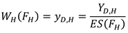
Equivalence scale-adjusted income serves as a measure of household welfare, enabling meaningful comparisons of well-being across households with varying sizes and compositions
Disposable income is a function of employment income , other income , benefits and taxes :
A vector of carbon intensity of each monetary unit of industrial production.
The carbon intensity of industry output represents the amount of carbon emissions produced per unit of monetary output in different industries. This vector helps measure the environmental impact of economic activities by linking industry production to emissions. It is commonly used in input-output analysis to assess the indirect carbon footprint of consumption and production processes. C be the carbon intensity vector (carbon emissions per unit of industry output), where each element represents the carbon emissions per monetary unit of output in industry i. E denote the vector of total emissions, where Eᵢ represents the total emissions from industry i. Let X be the vector of total output, where Xᵢ corresponds to the total monetary output of industry i. The carbon intensity vector can then be expressed as:
where each element is calculated as:
This approach determines emissions intensity per unit of output and is commonly applied in input-output analysis to estimate indirect emissions associated with both consumption and production.
Carbon Emissions Factors by Fuel Type
Each type of fuel has a unique emissions factor determined by its chemical makeup and energy content, typically measured in tCO₂/kWh. Biomass fuels like firewood are considered carbon-neutral if harvested sustainably. Among fossil fuels, coal has the highest carbon intensity due to its high carbon content and lower energy efficiency, while natural gas has the lowest, owing to its high hydrogen-to-carbon ratio. Diesel emits slightly more carbon than petrol because of its higher energy density. The carbon intensity of liquid fuels varies based on their composition and refining methods.
Total Emissions vs. Emissions Intensity
Distinguishing between total emissions and emissions intensity (emissions per unit of income) is essential for analyzing the distributional effects of carbon pricing. Total emissions represent the overall volume of greenhouse gases emitted, often linked to the scale of economic activity or energy use. In contrast, emissions intensity reflects the relative emissions burden in relation to income, revealing how carbon costs impact households and businesses across different income levels. Lower-income groups typically allocate a larger portion of their income to energy and carbon-intensive goods. As a result, despite having lower total emissions, they experience higher emissions intensity. This disparity means that carbon pricing policies tend to place a heavier financial burden on these groups, making emissions intensity a critical metric for evaluating distributional impacts and designing fair mitigation strategies.
Energy Intensity of Household Consumption
Household energy intensity, defined as energy consumption per unit of expenditure or income, plays a key role in evaluating the distributional effects of energy and carbon pricing policies. Lower-income households tend to have higher energy intensity since essential energy costs—such as heating, electricity, and transportation—make up a larger share of their total spending. Conversely, while higher-income households may consume more energy in absolute terms, energy accounts for a smaller proportion of their overall expenditures.
Heating Fuel Mix and Household Energy Costs
The mix of heating fuels—the blend of energy sources used for residential heating—significantly influences both household energy expenses and the distributional impact of carbon pricing. The cost of domestic energy per kWh is a crucial factor in determining energy affordability and how carbon pricing affects different income groups.
Effective Carbon Rates (ECR) Across Sectors and Fuel Types
Effective Carbon Rates (ECR), measured in currency units per ton of CO₂ emitted (tCO₂), vary across sectors and fuel types based on the OECD’s Effective Carbon Rates analysis. This framework classifies emissions by sector, including Agriculture & Fisheries, Buildings, Electricity, Industry, Off-road, and Road Transport, while also breaking down carbon pricing by fuel type, such as Coal, Fuel Oil, Kerosene, Natural Gas, Diesel, Gasoline, LPG, and other fossil fuels.
Direct Carbon Emissions from the Household Consumption
Direct carbon emissions from household consumption arise from activities such as burning fuels for heating, cooking, and personal transportation. These emissions are directly tied to household energy choices, including the use of electricity, natural gas, and fuels like gasoline or diesel.
In an input-output (IO) model, direct household emissions are estimated by applying emission factors to the final demand vector corresponding to household consumption. Specifically, emissions from each household activity are calculated by multiplying household expenditures on energy-intensive goods (represented in the final demand vector f ) by the direct emissions intensity for each sector (e).The total direct emissions where e is the direct emissions intensity vector that quantifies emissions per unit of output in each relevant sector, such as energy production, transportation, and heating. This formulation helps assess the direct carbon footprint of households and can guide policies aimed at reducing energy consumption and promoting cleaner technologies.
Indirect Carbon Emissions from the Household Consumption
Indirect carbon emissions stem from the production, transportation, and supply chain activities associated with the goods and services households consume. Although these emissions occur outside the household, they are driven by consumption choices.
To estimate indirect emissions, input-output (IO) models are commonly used, as they track carbon flows across different industries and capture the economic interconnections between sectors. This framework helps quantify the broader environmental impact of household consumption by considering emissions embedded in the production and distribution of goods and services. To estimate indirect carbon emissions from household consumption, we use an environmentally extended input-output (EEIO) model. Let E represent the vector of total sectoral emissions, A the technical coefficients matrix, and y the final demand vector representing household consumption. The Leontief inverse matrix, accounts for both direct and indirect effects across industries.
Decomposing the Distributional Impact of Carbon Taxation
The economy-wide emission intensity per unit of final demand is where γ is a row vector representing total emissions per unit of final demand; be the direct emissions intensity vector (1xn), where represents emissions per unit of output for sector i.
The total indirect carbon emissions from household consumption are:
The total indirect carbon emissions from household consumption are:
E is the total indirect carbon emissions from household consumption. The total emissions associated with household consumption can then be formulated as:
If disaggregated by household groups (e.g., by income deciles), household-specific final demand vectors can be used to compute emissions for different household types.
Decomposing the distributional impact of carbon taxation;
Disposable income after a carbon tax ():
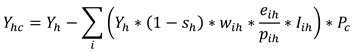
= savings rate
=“budget share of household expenditure allocated to expenditure group i”
= carbon intensity of expenditure category i expressed in t of CO2 per unit (kWh for energy goods2 and euro for non-energy goods)
= price per unit of energy paid by household ℎ
= indicator variable → household owns a carbon-emitting asset
= carbon price per ton of CO2
Equation (6) provides a framework for analyzing the distributional impact of carbon taxation by considering key drivers of household carbon emissions. One primary driver is household expenditure patterns, captured by the budget share . Households that allocate a higher proportion of their spending to energy-intensive goods and services will experience a greater reduction in disposable income due to carbon taxation. Another significant driver is the carbon intensity of consumption which varies by expenditure category. Energy goods, such as electricity and heating fuels, have higher direct carbon intensities, whereas non-energy goods contribute indirectly through supply chain emissions. The price per unit of energy further influences emissions, as households paying higher energy prices may be more incentivized to reduce consumption or switch to cleaner alternatives.
Household characteristics, such as ownership of carbon-emitting assets ,also shape emission levels. Households that own vehicles, use private transportation, or rely on fossil fuel-based heating systems will face a higher tax burden compared to those using cleaner technologies. Additionally, income and savings behavior play a role, as lower-income households tend to spend a larger share of their income on energy and have limited flexibility to adjust consumption in response to carbon price increases . This makes carbon taxation potentially regressive unless offset by revenue recycling or targeted support.
3. Methodology and Data
To capture the full impact of carbon emissions, we must account for both direct emissions and indirect emissions. This requires an Input-Output (IO) framework to trace emissions across the production chain. To assess the distributional effects of carbon pricing, Household Budget Survey (HBS) data provide valuable insights into how different income groups are impacted. By integrating these data with emissions estimation simulations, an input-output (IO) framework for indirect effects, and micro-level analysis to examine distributional impacts, we can create a thorough evaluation of how carbon pricing influences households across income levels
The study uses the PRICES (Prices, Revenue Recycling, Indirect Taxation, Carbon, Expenditure Simulation) microsimulation model (O’Donoghue et al., 2023), which can be used to simulate the effects of price increases from various sources, including external inflation shocks, changes in indirect taxes and environmental taxes. The PRICES framework offers two approaches to calculating CO2 emissions at sector level, providing a comprehensive tool for assessing the distributional and environmental impacts of tax policies. The first method applies an emissions vector from Corsatea et al. (2019), which takes into account both process-related and fugitive emissions in a country’s individual industries. The second, simpler approach calculates CO2 emissions from the energy industry and tracks energy consumption in each sector, focusing only on energy-related emissions and allowing simulations of carbon taxes based on energy consumption.The PRICES microsimulation model is structured as illustrated in Figure 2:
The methodological framework (Figure 2) contains,
Household Budget Survey (HBS) data, which captures consumption patterns and expenditure shares, enabling the assessment of fuel expenditures and the calculation of direct carbon emissions.
The Input-Output (I-O) database links sectoral economic data to household spending, estimating how price changes from fiscal policies, such as indirect and carbon taxes, impact expenditures
Ultimately, changes in income, prices, which shifts in consumption patterns influence emissions, reducing CO₂ output.
Data
The Household Budget Survey (HBS) 2019 was chosen over the Survey on Income and Living Conditions (SILC) because it provides detailed household expenditure data, which is essential for analyzing carbon pricing impacts and distributional effects. HBS is essential for analyzing consumption-based carbon emissions and the distributional effects of carbon pricing. Household Budget Survey (HBS) datasets provide detailed information on household expenditures by item, along with demographic, socioeconomic, and income data. The analysis uses the Turkish Household Budget Survey (HBS), collected by Statistics Turkey in 2019. To examine inter-industry relationships, the model incorporates the 2016 World Input-Output Database (WIOD) and its environmental extension, which includes industry-specific CO2 emissions data (Corsatea et al., 2019).
The focus of the analysis is on household consumption expenditure (as defined by Heinonen et al., 2020) to assess consumption-based carbon footprints (CF). A common approach for analyzing household CF is to combine HBS data with greenhouse gas (GHG) emissions intensities, as done in several countries including Finland (e.g., Ala-Mantila et al., 2014), Norway (Steen-Olsen et al., 2016), Germany (Gill and Moeller, 2018), and the Philippines (Seriño, 2017). Environmentally extended input-output (EEIO) models are frequently used to estimate consumption-based emissions intensities (e.g., Tukker and Jansen, 2006) and have been applied to evaluate impacts and prioritize policy measures to reduce GHG emissions and model lifestyle changes (Vita et al., 2019).
Input-output (IO) models and multiregional input-output (MRIO) models can be extended with environmental extensions to track the environmental impact of production processes across global supply chains. This leads to the development of environmentally extended input-output models (EEIO). These extensions account for the emissions or resource use linked to the production activities of various sectors across different regions. In the case of carbon emissions, EE-IO models create a connection between products and the indirect carbon emissions embedded in the production of goods and services. Kitzes (2013) presented the ecologically extended input-output analysis, while Minx et al. (2009) outlined its applications in estimating carbon footprints. It provides a valuable tool for analyzing changes in household consumption patterns, as shaped by national production technologies and emission intensities, and helps examine how income, demographics, and lifestyles influence variations in HCFs.
To model the indirect effects of producer price changes and carbon taxes, the pass-through of price changes to households is captured using an input-output (IO) table. Originally developed by Leontief (1951) and further refined in Miller and Blair (2009), IO modeling has been used in earlier studies such as O’Donoghue (1997) for Ireland, Gay and Proops (1993) in the United Kingdom, and Casler and Rafiqui (1993) to analyze the distributional effects of carbon taxation. More recent developments in distributional impact analysis, such as those by Sager (2019) and Feindt et al. (2021), use multi-regional IO (MRIO) models to further refine these assessments.
The central equation of our IO model, a Leontief quantity model, is the Leontief inverse matrix (I − A)−1, where is the identity matrix and is the technology matrix. The Leontief inverse gives the direct and indirect inter industry requirements for the economy:
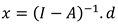
Transforming an IO model into an EE-IO requires a carbon intensity vector, capturing carbon emissions emitted by the industry in the production of a monetary unit of its output. Multiplying the Leontief inverse with the carbon intensity vector, we obtain a vector of the carbon intensity of each monetary unit of industrial production (, accounting for emissions released by the industry and by all downstream industries. Using bridging matrices we can translate the carbon emissions associated to industry outputs into indirect emissions associated to products consumed by households . To compute total household level emissions, we combined information on household fuel consumption with the carbon intensity of each fuel to create a vector of the household’s direct carbon emissions ( The sum of direct and indirect emissions gives households’ total carbon emissions associated to their consumption (:
Total emissions can be written as the product of the emission intensities per euro multiplied by the total expenditure for a given consumption category c,
where is a vector of (in-)direct emission intensities, expressed in kilograms of CO2 equivalent emissions per euro spent (kg CO2e/€), is a matrix of household expenditures (in €) for each household, capturing their associated spending patterns. This formulation allows for the calculation of household-level carbon footprints by linking emission intensities with specific expenditure data, enabling a detailed analysis of the environmental impact of consumption behaviors.
This study estimates household carbon footprints by combining Household Budget Survey (HBS) data with the World Input-Output Database (WIOD), mapping household consumption expenditures to emissions at the industry level. Since HBS follows the Classification of Individual Consumption by Purpose (COICOP) and WIOD utilizes ISIC rev. 4 or NACE rev. 2, a bridging matrix is necessary to connect consumption categories to industry outputs (Cai and Vandyck, 2020). For a more detailed explanation, refer to O’Donoghue et al. (2024).
4. Results
This section analyses household carbon emissions and energy consumption across income deciles, focusing on distributional impacts and energy affordability. It examines carbon emissions by fuel type, energy use and intensity, and domestic energy pricing and taxation. The results highlight differences in energy costs, tax burdens, and budget shares, showing how energy expenses affect households across income groups. Additionally, the comparison of direct and indirect emissions per expenditure provides insights into household carbon footprints and the equity implications of carbon pricing policies.
Different fuels have different carbon emissions depending upon their chemical structure. Different fuels emit varying amounts of carbon dioxide (CO₂) depending on their chemical composition and combustion characteristics. According to the Intergovernmental Panel on Climate Change (IPCC, 2019), coal has the highest carbon intensity, releasing approximately 90–100 kg of CO₂ per gigajoule (GJ) due to its high carbon content. Oil-based fuels, such as gasoline and diesel, emit less, typically around 70–75 kg CO₂/GJ, while natural gas, which consists primarily of methane (CH₄), has the lowest carbon intensity among fossil fuels, emitting approximately 50–55 kg CO₂/GJ. Biofuels, depending on their production process, may have lower net emissions due to carbon sequestration during biomass growth (Searchinger et al., 2008). The differences in carbon emissions across fuels play a crucial role in shaping climate policies and energy transition strategies (IEA, 2021).
Figure 3 illustrates fire wood has the highest carbon emissions per kWh among the fuels listed. While it is often considered a renewable resource, its high carbon emissions highlight the impact of inefficient burning and potential deforestation. Coal follows as the second-highest emitter, aligning with its reputation as a major contributor to global carbon emissions and reinforcing the push toward phasing out coal in favour of cleaner energy sources. Among fossil fuels, diesel, petrol, and liquid fuel show moderate emissions, with diesel being higher, often due to its use in industrial and heavy transportation sectors. Petrol, commonly used in transportation, has lower emissions than diesel and liquid fuel. Natural gas stands out as the lowest emitter among conventional fuels. It is often promoted as a transition fuel toward greener energy because of its relatively lower carbon footprint; however, methane leaks during extraction and transportation could undermine these benefits.
Analyzing carbon emissions by fuel type is necessary for designing effective, equitable, and targeted climate policies. It enables a better understanding of emission sources, helps identify distributional impacts, and supports the development of fuel-specific decarbonization strategies to achieve both environmental and social policy goals. Energy costs place a heavier financial burden on lower-income households Figure 4 highlights that lower-income deciles (1-3) exhibit higher energy intensity, meaning they use a larger proportion of their income on energy compared to higher-income groups. As income rises, the share of income spent on energy decreases, showcasing a falling share of income allocated to energy needs. The burden of energy costs is not equally distributed, as lower-income groups spend proportionally more on essential energy needs like home fuel and electricity, while higher-income groups have a greater proportion of their energy consumption in the motor fuel category, indicating more discretionary or mobility-related energy use.
Understanding the distributional impact of energy use is essential for developing policies that promote both equity and sustainability. Figure 5 illustrates the distributional impact of energy intensity, showing the ratio of energy consumption (kWh) to income across income deciles. The chart reveals an inverse relationship between income and energy intensity, with lower-income households (Decile 1) exhibiting significantly higher energy intensity. Decile 1’s high energy intensity is primarily driven by home fuel consumption, followed by electricity and motor fuel, indicating a large portion of their limited income goes toward basic energy needs. As income increases from Decile 2 to Decile 10, energy intensity decreases sharply. Higher-income groups consume more energy in absolute terms but allocate a smaller share of income to energy, reflecting their economic resilience. The blue segment (home fuel) dominates across all deciles but is most significant for lower-income groups, highlighting their reliance on energy for heating. Motor fuel (grey) becomes more prominent in middle-income deciles, reflecting greater mobility needs, while its share remains modest in higher-income deciles due to more energy-efficient transport options.
Addressing energy affordability and its impact on household budgets is crucial for fostering a fair and sustainable energy transition. Figure 6 illustrates the energy intensity of household consumption across income deciles, measured in kilowatt-hours (kWh) per unit of income. The chart highlights how lower-income households (Decile 1) have significantly higher energy intensity, meaning they spend a larger share of their income on energy consumption compared to wealthier households. As income increases, energy intensity declines, with the highest-income deciles (Decile 10) exhibiting the lowest energy usage relative to their income.
The chart categorizes energy consumption into three components:
Home Fuel (Blue): The dominant component, representing heating fuels like gas, coal, or wood.
Electricity (Orange): Covers household electricity consumption for appliances, lighting, and other uses.
Motor Fuel (Gray): Includes fuel used for personal transportation.
The figure reveals a regressive pattern, where low-income households bear a disproportionately higher energy burden. This suggests that energy cost policies, such as carbon taxes or subsidies, may have significant equity implications, particularly for vulnerable households.
Understanding the price of domestic energy per kWh across different equivalized disposable income deciles, as shown in Figure 7, is important for several reasons. It helps identify how energy costs are distributed across income groups and whether lower-income households pay higher prices for energy. Figure 7 shows that lower-income households (on the left side) pay more per kWh for heating fuel than higher-income households (on the right side). The price generally decreases as income increases, with some fluctuations in the middle deciles. This indicates a regressive pricing structure, where poorer households face a higher cost burden for energy, highlighting the need for more equitable pricing policies.
Effective Carbon Rates (ECRs) are essential for reflecting the true cost of carbon emissions, driving businesses and consumers to reduce their carbon footprint. By comparing ECRs across fuels and sectors, policymakers can identify carbon pricing gaps and craft fairer, more efficient environmental tax policies. Figure 8 illustrates the effective carbon rates across various sectors and fuel types, measured in currency units per ton of CO2 emitted (tCO2), based on the OECD’s Effective Carbon Rates (ECR) analysis. It categorizes emissions by sectors such as Agriculture & Fisheries, Buildings, Electricity, Industry, Off-road, and Road, and breaks down carbon rates by fuel types including Coal, Fuel Oil, Kerosene, Natural Gas, Diesel, Gasoline, LPG, and Other Fossil Fuels. Tax per tCO2 (Excise, ETS, Carbon Tax, 2021)
Figure 9, presents the budget share allocated to energy expenditures across different income deciles, with a focus on heating and electricity, motor fuel, and the ratio of home energy to motor fuels.
The x-axis represents equivalised expenditure deciles, ranging from the lowest (1st decile) to the highest (10th decile), while the left y-axis shows the budget share, and the right y-axis indicates the ratio of heating and electricity to motor fuels. The solid red line indicates the budget share for heating and electricity, the dashed red line represents motor fuel expenses, and the blue line shows the ratio of home energy to motor fuels. Key observations include:
Home Energy Concentration: The budget share for heating and electricity is significantly higher in the lowest income deciles, indicating that domestic fuel expenses are more concentrated at the very bottom of the income distribution.
Motor Fuel Profile: The budget share for motor fuels (dashed red line) is relatively flat in the middle of the income distribution, suggesting a more consistent expenditure pattern across these deciles.
Ratio of Home Energy to Motor Fuels: The blue line, showing the ratio of heating and electricity expenses to motor fuel costs, declines as income increases. This suggests that lower-income households allocate a much higher proportion of their energy budget to home heating and electricity than to motor fuels, compared to higher-income households.
Overall, the visualization highlights the regressive nature of home energy costs, with lower-income households facing a disproportionately high burden from heating and electricity expenses. Meanwhile, motor fuel expenses appear more evenly distributed across the middle-income deciles. The declining ratio of home energy to motor fuels with rising income further underscores the greater sensitivity of lower-income households to domestic energy costs.
Income-based disparities in spending patterns, showing how lower-income households allocate a much larger share of their income to essential goods like food and energy. Figure 10 shows the share of income spent on food, energy, and other expenses across income deciles. The lowest-income households (decile 1) spend a significantly larger share of their income on necessities than higher-income groups, making them more vulnerable to indirect taxation or price increases. As income rises, the proportion spent on essentials declines, reflecting greater financial flexibility among wealthier households. While energy costs (orange) are a smaller share overall, they remain a burden for low-income groups. Policy measures like carbon pricing or energy taxes could disproportionately affect lower-income households unless offset by subsidies or targeted transfers. Understanding these spending patterns is crucial for designing fiscal and environmental policies that avoid worsening inequality.
This graph highlights the distributional impact of carbon emissions across income groups, showing that direct emissions vary slightly with income, while indirect emissions are relatively constant. In the Figure 1, the blue line shows direct emissions from household energy use (fuel, heating, electricity), and the orange line represents indirect emissions embedded in goods and services (food, transport, manufactured goods). Direct emissions increase slightly with income, peaking in the middle deciles before declining at the highest levels, whereas indirect emissions remain relatively stable across all income groups. Higher-income households tend to produce more direct emissions due to greater energy consumption, such as larger homes and more vehicle use. This suggests that carbon pricing and energy taxes may have unequal effects across income groups, with higher-income households contributing more to direct emissions, while indirect emissions remain consistent across all deciles.
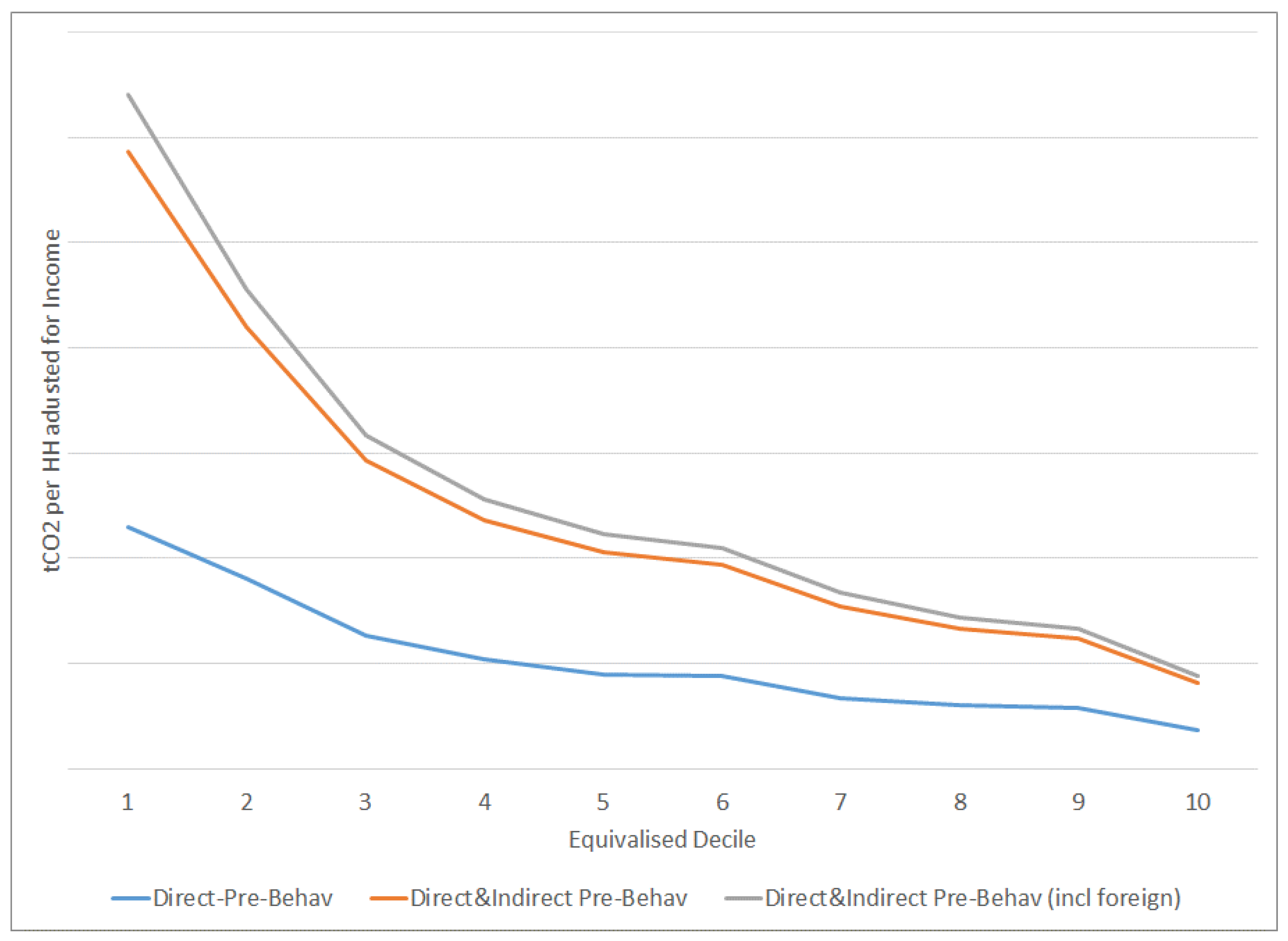
The graph aims to show how carbon pricing policies (like taxes or emissions trading) affect households at various income levels Figure 12 illustrates the carbon emissions per household expenditure, distinguishing between direct and indirect emissions across income deciles. The y-axis represents tons of CO₂ per household (adjusted for income), while the x-axis shows equivalized income deciles, from the lowest-income group (Decile 1) to the highest-income group (Decile 10).
The analysis of household emissions across income deciles reveals distinct patterns. Direct emissions (blue line) from fuel use, such as heating and transportation, are most intense in lower-income households (Decile 1) and decrease with higher income. Including indirect emissions (orange line) from goods and services, the trend remains similar, with intensity declining across deciles. When foreign supply chain emissions (gray line) are added, higher-income deciles show increased emissions due to greater consumption of imported goods. This highlights the regressive nature of energy taxation on lower-income households and the global impact of consumption-driven emissions in wealthier deciles. Policymakers must design targeted interventions to address these disparities, balancing direct and indirect carbon footprints while considering the broader implications of consumption patternsLower-income households have higher emissions per unit of expenditure, largely due to a greater reliance on carbon-intensive fuels for essential needs. Higher-income households have lower emissions per unit of expenditure but contribute more to total emissions, particularly through indirect and foreign-related emissions. This suggests that carbon pricing policies need to consider both direct household energy consumption and indirect emissions from consumption patterns, particularly in wealthier households.
5. Discussion and Conclusions
This paper examines the distributional drivers of carbon emissions in Türkiye, focusing on how different income groups contribute to carbon footprints. The study reveals significant disparities in carbon emissions across income deciles, showing the complex relationship between household income, consumption patterns, and environmental impact.
Lower-income households exhibit higher energy intensity, meaning they spend a larger proportion of their income on essential energy needs such as heating and electricity. This disproportionate expenditure highlights the vulnerability of these households to energy poverty, especially when energy prices rise due to carbon pricing policies. In contrast, while higher-income households consume more energy overall, they allocate a smaller share of their income to energy, which reflects their greater economic resilience. However, these households also contribute significantly to indirect emissions, primarily due to their consumption of energy-intensive goods and services, particularly imported products. This indicates that affluent consumption patterns have a broader environmental impact, beyond direct energy consumption.
The study emphasizes the distinction between direct and indirect emissions. Direct emissions, which primarily arise from home heating and personal transportation, are more prevalent among lower-income households, who rely on carbon-heavy fuels. Indirect emissions, on the other hand, are linked to the production and supply chain of consumed goods and services. These emissions are more significant in higher-income households due to their consumption of imported products. This duality in emissions underscores the need for policies that address both direct energy use and the wider environmental effects of consumption.
Middle-income countries, like Türkiye, face the challenge of balancing economic growth with emission reductions. Rising incomes and a growing middle class drive higher demand for energy-intensive goods and services, which could increase fossil fuel consumption. To mitigate this, policies promoting renewable energy, energy efficiency, and cleaner transportation are crucial. Targeted measures, such as energy subsidies and income support programs, are necessary to protect lower-income households from the regressive impacts of carbon pricing, ensuring energy equity.
In Türkiye, energy tax policy uses excise duties to regulate energy consumption. The rates vary across fuels and sectors, with some fuels benefiting from lower taxes or higher subsidies, particularly heating fuels. Türkiye’s Emissions Trading Scheme (ETS) aims to reduce greenhouse gas emissions through a market-driven approach. The introduction of a carbon tax could disproportionately impact lower-income households, as they spend a higher share of their income on energy costs that offer limited flexibility for reduction. In contrast, higher-income households may adapt by reducing discretionary energy use, such as motor fuel.
As middle-income countries see a growing middle class and rising energy demands, they face the challenge of managing energy consumption without undermining climate goals. The World Energy 2017-2050 report emphasizes that these countries are at a crossroads. To avoid increasing fossil fuel consumption, policies should prioritize renewable energy investments, energy efficiency improvements, and cleaner transportation solutions. Additionally, targeted subsidies and support programs for lower-income groups are necessary to shield them from the regressive impacts of carbon pricing.
This study offers valuable insights into the distributional factors that drive carbon emissions in Türkiye, highlighting the need for equitable and effective carbon pricing mechanisms. Carbon pricing disproportionately affects lower-income households, who spend a larger share of their income on energy. Compensatory measures, such as subsidies, income support, or energy efficiency programs, are essential to alleviate the burden on vulnerable populations and ensure a just transition to a low-carbon economy.
Higher-income households contribute significantly to indirect emissions, particularly through the consumption of energy-intensive and imported goods. Policies should target these consumption patterns by promoting energy-efficient technologies, sustainable practices, and investments in renewable energy. A comprehensive strategy that addresses both direct and indirect emissions is crucial. Policymakers should prioritize investments in public transportation, energy-efficient housing, and cleaner mobility solutions to reduce fossil fuel dependence and encourage sustainable consumption.
Rising middle classes in middle-income countries present a unique challenge in managing the demand for energy-intensive goods without exacerbating fossil fuel consumption. Policies should focus on balancing economic growth with emissions reductions, promoting renewable energy, and enhancing energy efficiency, particularly in urban and transport sectors.
In conclusion, by addressing both direct and indirect emissions and tailoring interventions to the needs of different income groups, it is possible to reduce carbon emissions significantly while promoting social equity and economic resilience. Policymakers in Türkiye can use these insights to develop more equitable and effective carbon pricing strategies that support both environmental and social goals.
References
- Ala-Mantila, S.; Heinonen, J.; Junnila, S. Relationship between urbanization, direct and indirect greenhouse gas emissions, and expenditures: A multivariate analysis. Ecological Economics 2014, 104, 129–139. [Google Scholar]
- Alexander-Haw, A.; Schleich, J. Low carbon footprint-A consequence of free will or of poverty? The impact of sufficiency orientation and deprivation on individual carbon footprints. Energy Policy 2024, 195, 114367. [Google Scholar]
- Baiocchi, G.; Minx, J.; Hubacek, K. The impact of social factors and consumer behavior on carbon dioxide emissions in the United Kingdom: A regression based on input? output and geodemographic consumer segmentation data. Journal of Industrial Ecology 2010, 14, 50–72. [Google Scholar]
- Baker, P.; Blundell, R.; Micklewright, J. Modelling household energy expenditures using micro-data. The Economic Journal 1989, 99, 720–738. [Google Scholar]
- Benders, R.M.; Moll, H.C.; Nijdam, D.S. From energy to environmental analysis: Improving the resolution of the environmental impact of Dutch private consumption with hybrid analysis. Journal of Industrial Ecology 2012, 16, 163–175. [Google Scholar]
- Benders, R.M.; Moll, H.C.; Nijdam, D.S. From energy to environmental analysis: Improving the resolution of the environmental impact of Dutch private consumption with hybrid analysis. Journal of Industrial Ecology 2012, 16, 163–175. [Google Scholar]
- Buchs, M.; Schnepf, S.V. (2013). UK households’ carbon footprint: a comparison of the association between household characteristics and emissions from home energy, transport and other goods and services (No. 7204). IZA Discussion Papers.
- Caeiro, S.; Ramos, T.B.; Huisingh, D. Procedures and criteria to develop and evaluate household sustainable consumption indicators. Journal of Cleaner Production 2012, 27, 72–91. [Google Scholar] [CrossRef]
- Cai, M.; Vandyck, T. Bridging between economy-wide activity and household-level consumption data: Matrices for European countries. Data in Brief 2020, 30, 105395. [Google Scholar]
- Can, Z.G.; O’Donoghue, C.; Sologon, D. (2025). The Distributional Effects of Carbon Pricing in Türkiye. IZA DISCUSSION PAPER SERIES IZA DP No. 17701.
- Casler, S.D.; Rafiqui, A. Evaluating fuel tax equity: Direct and indirect distributional effects. National Tax Journal 1993, 46, 197–205. [Google Scholar]
- Cazcarro, I.; Amores, A.F.; Arto, I.; Kratena, K. Linking multisectoral economic models and consumption surveys for the European Union. Economic Systems Research 2022, 34, 22–40. [Google Scholar] [CrossRef]
- Chitnis, M.; Sorrell, S.; Druckman, A.; Firth, S.K.; Jackson, T. Who rebounds most? Estimating direct and indirect rebound effects for different UK socioeconomic groups. Ecological Economics 2014, 106, 12–32. [Google Scholar]
- Choi, K.; Zhang, M. The net effects of the built environment on household vehicle emissions: A case study of Austin, TX. Transportation Research Part D: Transport and Environment 2017, 50, 254–268. [Google Scholar]
- Corsatea, T.D.; Lindner, S.; Arto, I.; Román, M.V.; Rueda-Cantuche, J.M.; Velázquez Afonso, A. ; .. & Neuwahl, F. World input-output database environmental accounts. Update 2000, 2016, 54. [Google Scholar]
- Coruh, E.; Bilgic, A.; Cengiz, V.; Urak, F. Uncovering the determinants of bottom-up CO2 emissions among households in Türkiye: Analysis and policy recommendations. Journal of Cleaner Production 2024, 469, 143197. [Google Scholar]
- Coruh, E.; Bilgic, A.; Cengiz, V.; Urak, F. Uncovering the determinants of bottom-up CO2 emissions among households in Türkiye: Analysis and policy recommendations. Journal of Cleaner Production 2024, 469, 143197. [Google Scholar] [CrossRef]
- Creedy, J. Lifetime versus annual income distribution. In Handbook of Income Inequality Measurement 1999, 513-534. Dordrecht: Springer Netherlands.
- Csutora, M. One more awareness gap? The behaviour-impact gap problem. Journal of Consumer Policy 2012, 35, 145–163. [Google Scholar]
- Dogan, E.; Madaleno, M.; Taskin, D. Which households are more energy vulnerable? Energy poverty and financial inclusion in Turkey. Energy Economics 2021, 99, 105306. [Google Scholar]
- Dorband, I.I.; Jakob, M.; Kalkuhl, M.; Steckel, J.C. Poverty and distributional effects of carbon pricing in low-and middle-income countries–A global comparative analysis. World Development 2019, 115, 246–257. [Google Scholar]
- Druckman, A.; Jackson, T. The carbon footprint of UK households 1990-2004: a Socio-economically disaggregated, Quasi-multi-regional input-output model. Ecological economics 2009, 68. [Google Scholar] [CrossRef]
- Druckman, A.; Jackson, T. Understanding households as drivers of carbon emissions. Taking Stock of Industrial Ecology 2016, 181–203. [Google Scholar]
- Dubois, G.; Sovacool, B.; Aall, C.; Nilsson, M.; Barbier, C.; Herrmann, A. ; .. & Sauerborn, R. It starts at home? Climate policies targeting household consumption and behavioral decisions are key to low-carbon futures. Energy Research & Social Science 2019, 52, 144–158. [Google Scholar]
- Elgouacem, A.; Immervoll, H.; Raj, A.; Linden, J.; O’Donoghue, C.; Sologon, D.M. (2024). Who pays for higher carbon prices? Mitigating climate change and adverse distributional effects. In OECD Employment Outlook 2024: The Net-Zero Transition and the Labour Market (pp. 226–268). OECD.
- Elgouacem, A.; Immervoll, H.; Raj, A.; Linden, J.; O’Donoghue, C.; Sologon, D.M. (2024). Who pays for higher carbon prices? Mitigating climate change and adverse distributional effects. In OECD Employment Outlook 2024: The Net-Zero Transition and the Labour Market (pp. 226–268). OECD.
- Feindt, S.; Kornek, U.; Labeaga, J.M.; Sterner, T.; Ward, H. Understanding regressivity: Challenges and opportunities of European carbon pricing. Energy Economics 2021, 103, 105550. [Google Scholar]
- Fremstad, A.; Underwood, A.; Zahran, S. The environmental impact of sharing: Household and urban economies in CO2 emissions. Ecological Economics 2018, 145, 137–147. [Google Scholar]
- Gay, P.W.; Proops, J.L. Carbon-dioxide production by the UK economy: An input-output assessment. Applied Energy 1993, 44, 113–130. [Google Scholar]
- Gevrek, Z.E.; Uyduranoglu, A. Public preferences for carbon tax attributes. Ecological Economics 2015, 118, 186–197. [Google Scholar]
- Gill, B.; Moeller, S. GHG emissions and the rural-urban divide. A carbon footprint analysis based on the German official income and expenditure survey. Ecological Economics 2018, 145, 160–169. [Google Scholar]
- Golley, J.; Meng, X. Income inequality and carbon dioxide emissions: The case of Chinese urban households. Energy Economics 2012, 34, 1864–1872. [Google Scholar] [CrossRef]
- Gough, I.; Abdallah, S.; Johnson, V.; Ryan-Collins, J.; Smith, C. (2011). The distribution of total greenhouse gas emissions by households in the UK, and some implications for social policy. LSE STICERD Research Paper No. CASE152.
- Han, L.; Xu, X.; Han, L. Applying quantile regression and Shapley decomposition to analyzing the determinants of household embedded carbon emissions: evidence from urban China. Journal of Cleaner Production 2015, 103, 219–230. [Google Scholar]
- Heinonen, J.; Jalas, M.; Juntunen, J.K.; Ala-Mantila, S.; Junnila, S. Situated lifestyles: II. The impacts of urban density, housing type and motorization on the greenhouse gas emissions of the middle-income consumers in Finland. Environmental Research Letters 2013, 8, 035050. [Google Scholar]
- Heinonen, J.; Ottelin, J.; Ala-Mantila, S.; Wiedmann, T.; Clarke, J.; Junnila, S. Spatial consumption-based carbon footprint assessments-A review of recent developments in the field. Journal of Cleaner Production 2020, 256, 120335. [Google Scholar] [CrossRef]
- Hertwich, E.G.; Peters, G.P. Carbon footprint of nations: a global, trade-linked analysis. Environmental science & technology 2009, 43, 6414–6420. [Google Scholar]
- International Energy Agency (IEA). (2021). Turkey 2021 Energy Policy Review.
- Ivanova, D.; Barrett, J.; Wiedenhofer, D.; Macura, B.; Callaghan, M.; Creutzig, F. Quantifying the potential for climate change mitigation of consumption options. Environmental Research Letters 2020, 15, 093001. [Google Scholar] [CrossRef]
- Ivanova, D.; Stadler, K.; Steen?Olsen, K.; Wood, R.; Vita, G.; Tukker, A.; Hertwich, E.G. Environmental impact assessment of household consumption. Journal of Industrial Ecology 2016, 20, 526–536. [Google Scholar] [CrossRef]
- Ivanova, D.; Vita, G.; Steen-Olsen, K.; Stadler, K.; Melo, P.C.; Wood, R.; Hertwich, E.G. Mapping the carbon footprint of EU regions. Environmental Research Letters 2017, 12, 054013. [Google Scholar] [CrossRef]
- Jakob, M.; Steckel, J.; Klasen, S.; et al. Feasible mitigation actions in developing countries. Nature Clim Change 2014, 4, 961–968. [Google Scholar] [CrossRef]
- Jones, C.M.; Kammen, D.M. Quantifying carbon footprint reduction opportunities for US households and communities. Environmental Science & Technology 2011, 45, 4088–4095. [Google Scholar]
- Jones, C.; Kammen, D.M. Spatial distribution of US household carbon footprints reveals suburbanization undermines greenhouse gas benefits of urban population density. Environmental Science & Technology 2014, 48, 895–902. [Google Scholar]
- Kerkhof, A.C.; Benders, R.M.; Moll, H.C. Determinants of variation in household CO2 emissions between and within countries. Energy Policy 2009, 37, 1509–1517. [Google Scholar] [CrossRef]
- Kitzes, J. An introduction to environmentally-extended input-output analysis. Resources 2013, 2, 489–503. [Google Scholar] [CrossRef]
- Larsen, H.N.; Hertwich, E.G. Implementing Carbon-Footprint-Based Calculation Tools in Municipal Greenhouse Gas Inventories: The Case of Norway. Journal of Industrial Ecology 2010, 14, 965–977. [Google Scholar] [CrossRef]
- Leontief, W.W. ; Input-output economics. Scientific American 1951, 185, 15–21. [Google Scholar]
- Lévay, P.Z.; Vanhille, J.; Goedemé, T.; Verbist, G. The association between the carbon footprint and the socio-economic characteristics of Belgian households. Ecological Economics 2021, 186, 107065. [Google Scholar]
- Li, J.; Huang, X.; Yang, H.; Chuai, X.; Li, Y.; Qu, J.; Zhang, Z. Situation and determinants of household carbon emissions in Northwest China. Habitat Int. 2016, 51, 178–187. [Google Scholar] [CrossRef]
- Li, M. (2017). World energy 2017-2050: Annual report. Department of Economics, University of Utah.
- Linden, J.; O’Donoghue, C.; Sologon, D.M. The many faces of carbon tax regressivity-Why carbon taxes are not always regressive for the same reason. Energy Policy 2024, 192, 114210. [Google Scholar]
- Matthews, H.S.; Hendrickson, C.T.; Weber, C.L. The importance of carbon footprint estimation boundaries Environ. Sci. Technol. 2008, 42, 5839–5842. [Google Scholar]
- Miller, R.E.; Blair, P.D. (2009). Input-output analysis: foundations and extensions. Cambridge university press.
- Minx, J.C.; Wiedmann, T.; Wood, R.; Peters, G.P.; Lenzen, M.; Owen, A. ; .. & Ackerman, F. Input-output analysis and carbon footprinting: An overview of applications. Economic Systems Research 2009, 21, 187–216. [Google Scholar]
- Minx, J.; Baiocchi, G.; Wiedmann, T.; Barrett, J.; Creutzig, F.; Feng, K. ; .. & Hubacek, K. Carbon footprints of cities and other human settlements in the UK. Environmental Research Letters 2013, 8, 035039. [Google Scholar]
- Mongelli, I.; Neuwahl, F.; Rueda-Cantuche, J.M. Integrating a household demand system in the input-output framework. Methodological aspects and modelling implications. Economic Systems Research 2010, 22, 201–222. [Google Scholar]
- Moser, S.; Kleinhückelkotten, S. Good intents, but low impacts: diverging importance of motivational and socioeconomic determinants explaining pro-environmental behavior, energy use, and carbon footprint. Environment and Behavior 2018, 50, 626–656. [Google Scholar]
- Nässén, J.; Andersson, D.; Larsson, J.; Holmberg, J. Explaining the variation in greenhouse gas emissions between households: socioeconomic, motivational, and physical factors. Journal of Industrial Ecology 2015, 19, 480–489. [Google Scholar]
- O’Donoghue, C. (1997). Carbon Dioxide, Energy Taxes and Household Income. ESRI WP90. November 1997.
- O’Donoghue, C.; Amjad, B.; Linden, J.; Lustig, N.; Sologon, D.; Wang, Y. (2023). The distributional Impact of a Price Inflation in Pakistan: A Case Study of a New Price Focused Microsimulation Framework, PRICES. LISER Working Paper Series. Luxembourg Institute of Socio-Economic Research (LISER).
- OECD Employment Outlook.
- Ottelin, J.; Ala-Mantila, S.; Heinonen, J.; Wiedmann, T.; Clarke, J.; Junnila, S. What can we learn from consumption-based carbon footprints at different spatial scales? Review of policy implications. Environmental Research Letters 2019, 14, 093001. [Google Scholar]
- Poom, A.; Ahas, R. How does the environmental load of household consumption depend on residential location? . Sustainability 2016, 8, 799. [Google Scholar] [CrossRef]
- Qu, J.; Zeng, J.; Li, Y.; Wang, Q.; Maraseni, T.; Zhang, L. ; .. & Clarke-Sather, A. Household carbon dioxide emissions from peasants and herdsmen in northwestern arid-alpine regions, China. Energy Policy 2013, 57, 133–140. [Google Scholar]
- Renner, S. Poverty and distributional effects of a carbon tax in Mexico. Energy Policy 2018, 112, 98–110. [Google Scholar] [CrossRef]
- Saelim, S. Carbon tax incidence on household consumption: Heterogeneity across socio-economic factors in Thailand. Economic Analysis and Policy 2019, 62, 159–174. [Google Scholar] [CrossRef]
- Sager, L. Income inequality and carbon consumption: Evidence from Environmental Engel curves. Energy Economics 2019, 84, 104507. [Google Scholar] [CrossRef]
- Schaltegger, S.; Csutora, M. Carbon accounting for sustainability and management. Status quo and challenges. Journal of cleaner production 2012, 36, 1–16. [Google Scholar] [CrossRef]
- Seriño, M.N. V. Is decoupling possible? Association between affluence and household carbon emissions in the Philippines. Asian Economic Journal 2017, 31, 165–185. [Google Scholar]
- Seriño, M.N. V.; Klasen, S. Estimation and Determinants of the P hilippines’ Household Carbon Footprint. The Developing Economies 2015, 53, 44–62. [Google Scholar] [CrossRef]
- Shei, C.H.; Liu, J.C. E.; Hsieh, I.Y. L. Distributional effects of carbon pricing: An analysis of income-based versus expenditure-based approaches. Journal of Cleaner Production 2024, 141446. [Google Scholar] [CrossRef]
- Steckel, J.C. (2012). Developing Countries in the Context of Climate Change Mitigation and Energy System Transformation.
- Steckel, J.C.; Dorband, I.I.; Montrone, L.; Ward, H.; Missbach, L.; Hafner, F. ; .. & Renner, S. Distributional impacts of carbon pricing in developing Asia. Nature Sustainability 2021, 4, 1005–1014. [Google Scholar]
- Steen?Olsen, K.; Wood, R.; Hertwich, E.G. The carbon footprint of Norwegian household consumption 1999-2012. Journal of Industrial Ecology 2016, 20, 582–592. [Google Scholar]
- Tukker, A.; Jansen, B. Environmental impacts of products: A detailed review of studies. Journal of Industrial Ecology 2006, 10, 159–182. [Google Scholar]
- Turkish Statistical Institute (TURKSTAT). (2022). Final Energy Consumption Statistics in Households, 2022, Available https://www.tuik.gov.tr/Home/Index.
- Uzar, U.; Eyuboglu, K. The nexus between income inequality and CO2 emissions in Turkey. Journal of Cleaner Production 2019, 227, 149–157. [Google Scholar]
- Vita, G.; Ivanova, D.; Dumitru, A.; García-Mira, R.; Carrus, G.; Stadler, K. ; .. & Hertwich, E.G. Happier with less? Members of European environmental grassroots initiatives reconcile lower carbon footprints with higher life satisfaction and income increases. Energy Research & Social Science 2020, 60, 101329. [Google Scholar]
- Vita, G.; Lundström, J.R.; Hertwich, E.G.; Quist, J.; Ivanova, D.; Stadler, K.; Wood, R. The environmental impact of green consumption and sufficiency lifestyles scenarios in Europe: connecting local sustainability visions to global consequences. Ecological Economics 2019, 164, 106322. [Google Scholar]
- Wang, K.; Cui, Y.; Zhang, H.; Shi, X.; Xue, J.; Yuan, Z. Household carbon footprints inequality in China: Drivers, components and dynamics. Energy Economics 2022, 115, 106334. [Google Scholar] [CrossRef]
- Weber, C.L.; Matthews, H.S. Quantifying the global and distributional aspects of American household carbon footprint. 2008, 66(2-3), 379-391. Ecological Economics 2008, 66, 379–391. [Google Scholar]
- Wiedenhofer, D.; Guan, D.; Liu, Z.; Meng, J.; Zhang, N.; Wei, Y.M. Unequal household carbon footprints in China. Nature Climate Change 2017, 7, 75–80. [Google Scholar]
- Wiedenhofer, D.; Smetschka, B.; Akenji, L.; Jalas, M.; Haberl, H. Household time use, carbon footprints, and urban form: a review of the potential contributions of everyday living to the 1. 5 C climate target. Current Opinion in Environmental Sustainability 2018, 30, 7–17. [Google Scholar] [CrossRef]
- Wier, M.; Lenzen, M.; Munksgaard, J.; Smed, S. Effects of household consumption patterns on CO2 requirements. Economic Systems Research 2001, 13, 259–274. [Google Scholar] [CrossRef]
- World Data Lab, Available https://worlddatalab.com/.
- World Emissions Clock, Available https://worldemissions.io/.
- Xie, J.; Zhou, S.; Teng, F.; Gu, A. The characteristics and driving factors of household CO2 and non-CO2 emissions in China. Ecological Economics 2023, 213, 107952. [Google Scholar] [CrossRef]
- Yan, J.; Yang, J. Carbon pricing and income inequality: A case study of Guangdong Province, China. Journal of Cleaner Production 2021, 296, 126491. [Google Scholar] [CrossRef]
- Zeng, J.; Qu, J.; Ma, H.; Gou, X. Characteristics and Trends of household carbon emissions research from 1993 to 2019: A bibliometric analysis and its implications. Journal of Cleaner Production 2021, 295, 126468. [Google Scholar] [CrossRef]
- Zhang, J.; Terrones, M.; Park, C.R.; Mukherjee, R.; Monthioux, M.; Koratkar, N. ; .. & Bianco, A. Carbon science in 2016: Status, challenges and perspectives. Carbon 2016, 98, 708–732. [Google Scholar]
- Zhang, Y.; Jiang, S.; Lin, X.; Qi, L.; Sharp, B. Income distribution effect of carbon pricing mechanism under China’s carbon peak target: CGE-based assessments. Environmental Impact Assessment Review 2023, 101, 107149. [Google Scholar]
Figure 1.
Structure of Household Consumption Decisions. Source: Authors’ elaboration.
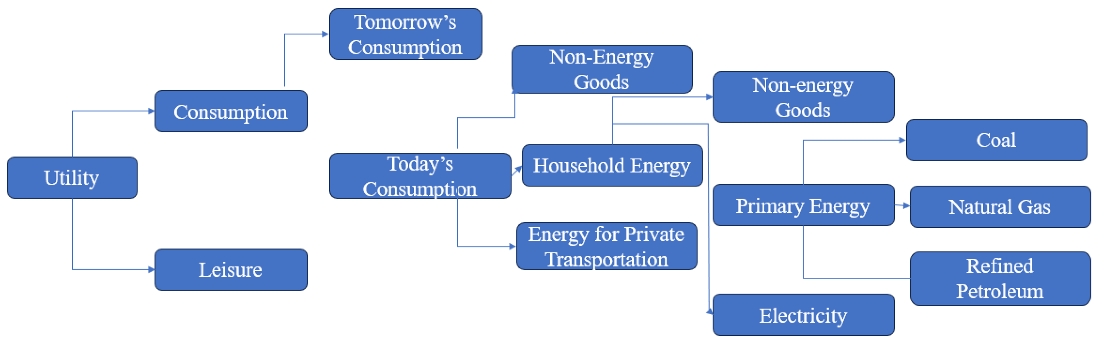
Figure 2.
Microsimulation Model Framework. Source: Modelling the distributional impact of a carbon tax requires therefore both micro units and a simulation framework, known as a microsimulation model (Hynes and O’Donoghue, 2014; O’Donoghue, 2021).
Figure 2.
Microsimulation Model Framework. Source: Modelling the distributional impact of a carbon tax requires therefore both micro units and a simulation framework, known as a microsimulation model (Hynes and O’Donoghue, 2014; O’Donoghue, 2021).
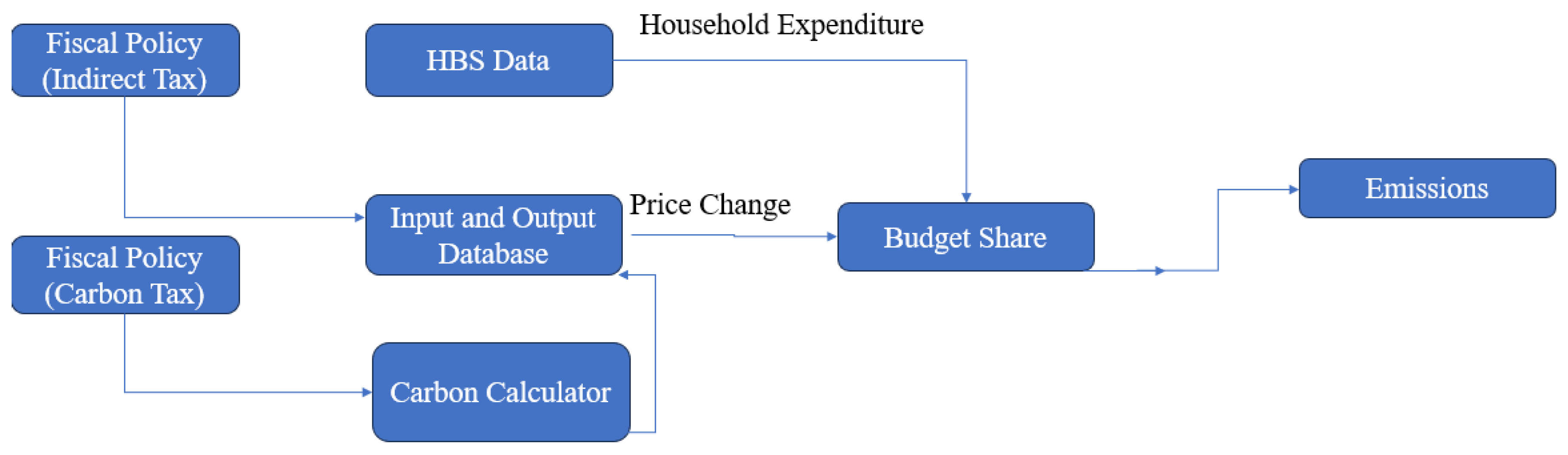
Figure 3.
Carbon Emissions by Fuel Type (Emissions (tCO2) per kwh).
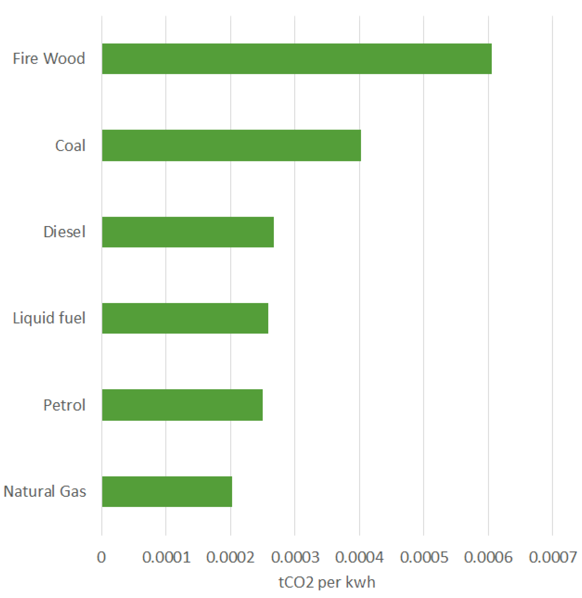
Figure 4.
Distributional impact of energy use (Kwh per equivalent adult by decile).
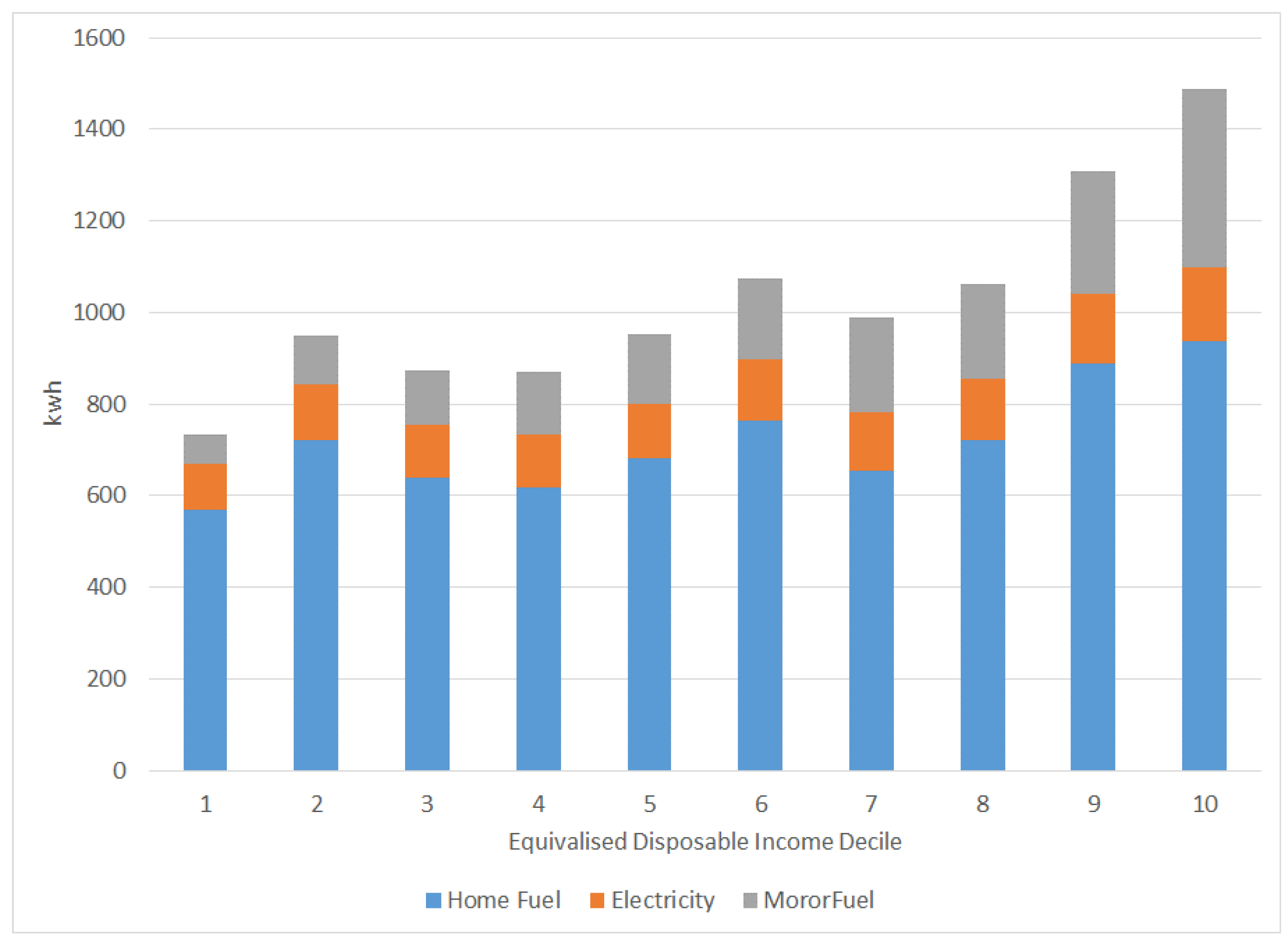
Figure 5.
Distributional impact of energy intensity (Energy intensity (kwh) by decile.
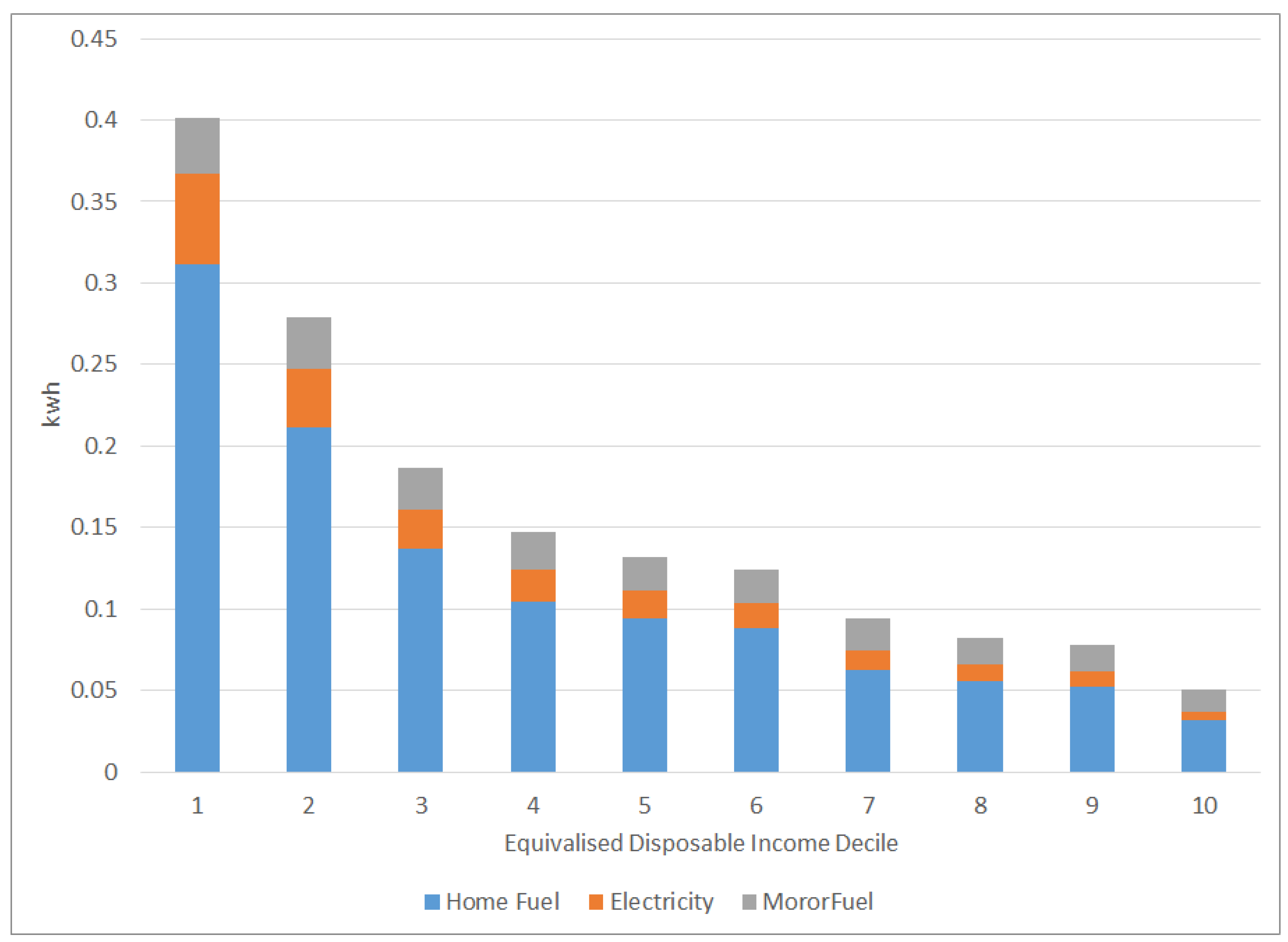
Figure 6.
Heating fuel mix.
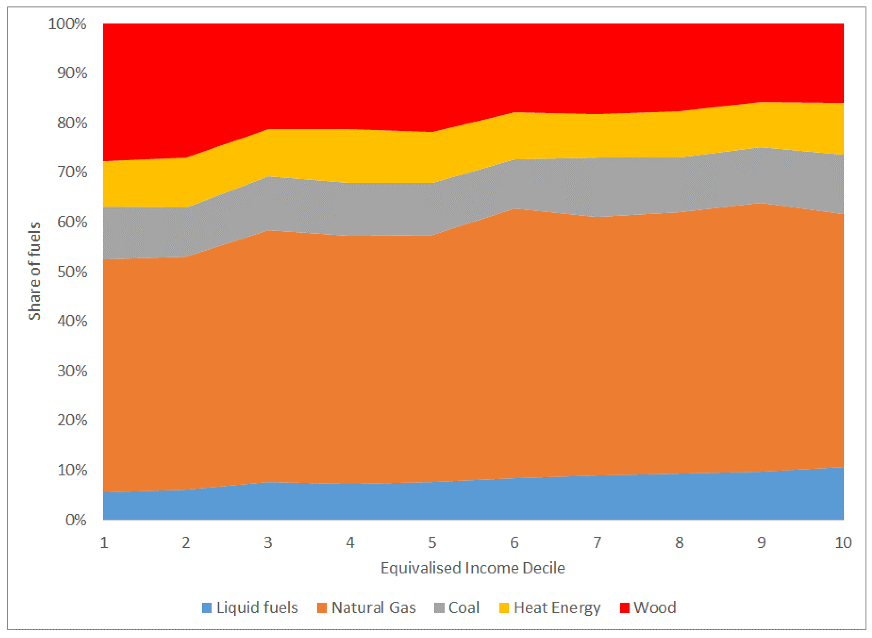
Figure 7.
Price of domestic energy (per kwh by decile).
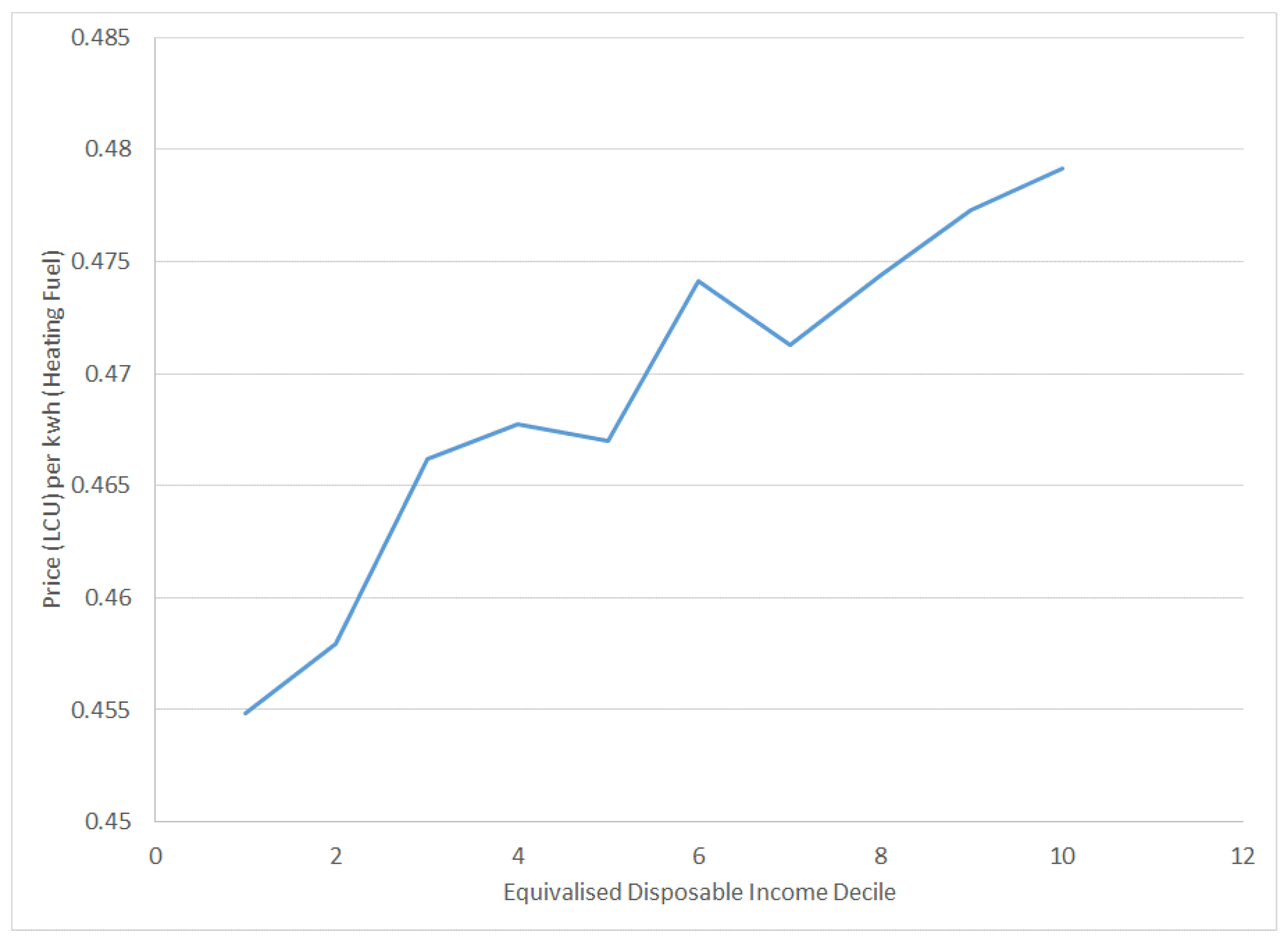
Figure 8.
Tax per tCO2 (Excise, ETS, Carbon tax, 2021).
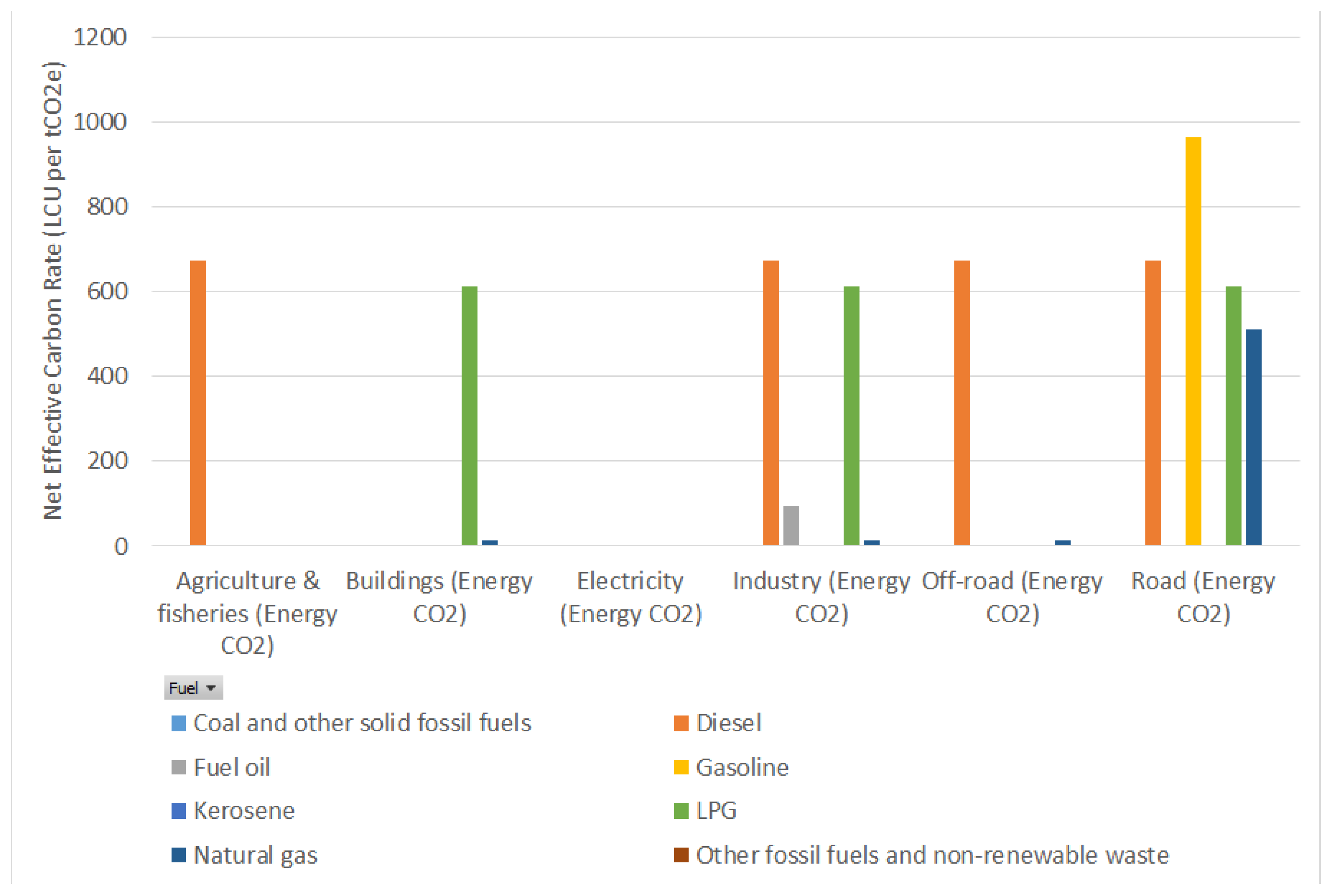
Figure 9.
Budget share in income for energy by decile.
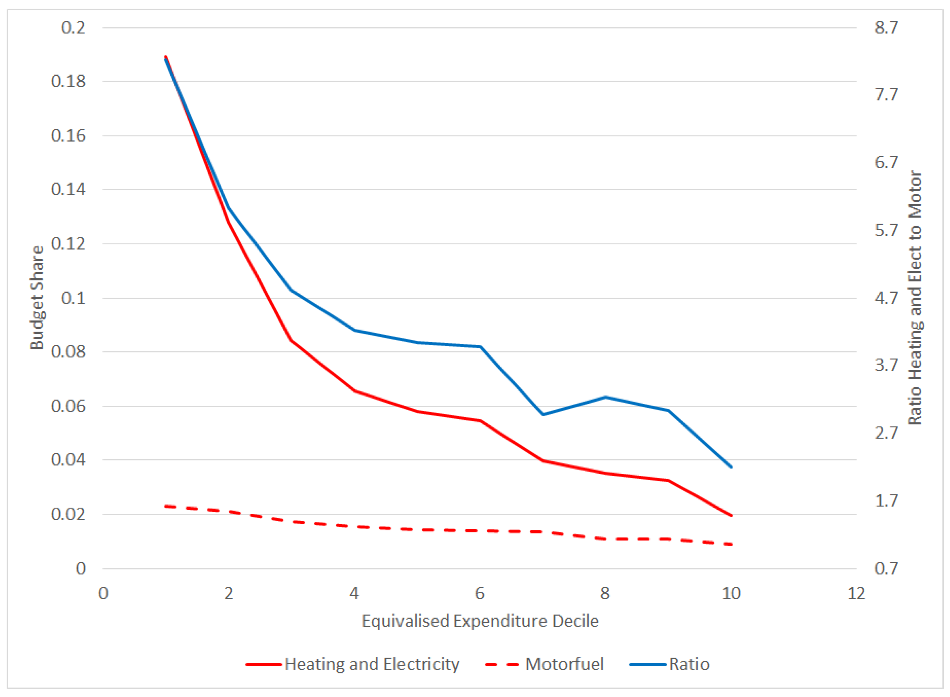
Figure 10.
Budget share in income for energy by decile.
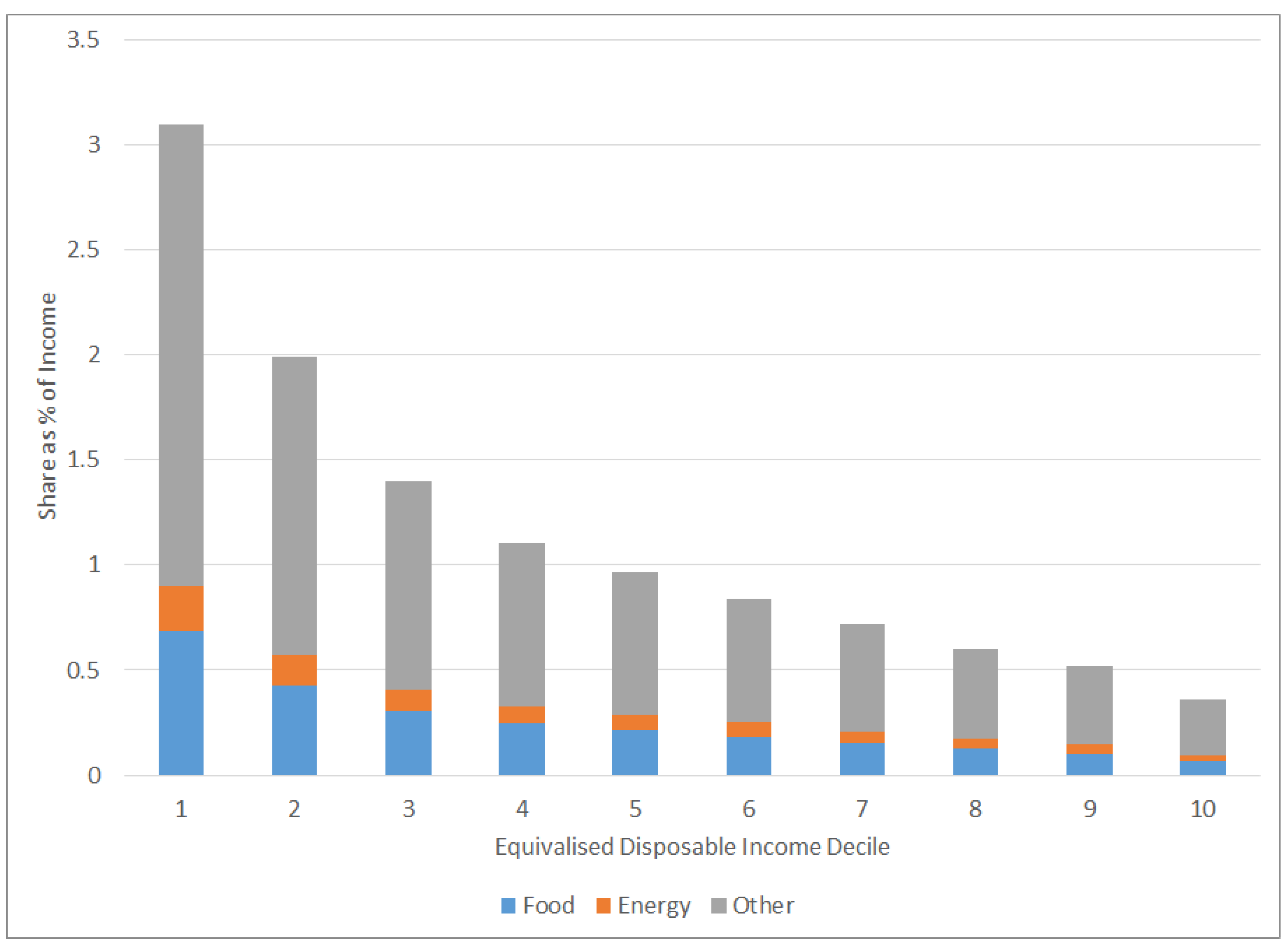
Figure 11.
Emissions per expenditure direct vs indirect.
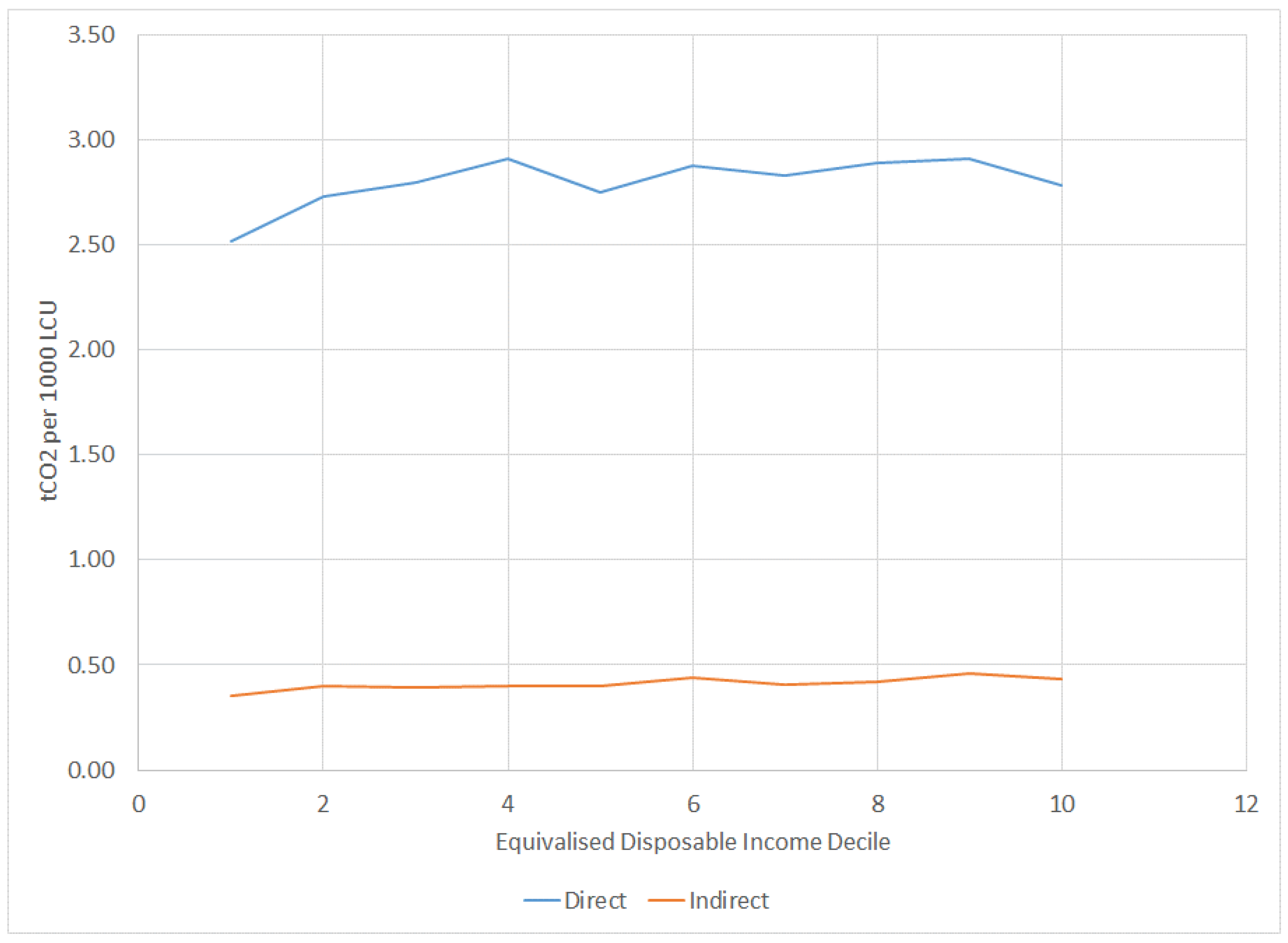
Figure 12.
Emissions per expenditure (direct vs indirect).
Disclaimer/Publisher’s Note: The statements, opinions and data contained in all publications are solely those of the individual author(s) and contributor(s) and not of MDPI and/or the editor(s). MDPI and/or the editor(s) disclaim responsibility for any injury to people or property resulting from any ideas, methods, instructions or products referred to in the content. |
© 2025 by the authors. Licensee MDPI, Basel, Switzerland. This article is an open access article distributed under the terms and conditions of the Creative Commons Attribution (CC BY) license (http://creativecommons.org/licenses/by/4.0/).
Copyright: This open access article is published under a Creative Commons CC BY 4.0 license, which permit the free download, distribution, and reuse, provided that the author and preprint are cited in any reuse.


