
Submitted:
27 March 2025
Posted:
28 March 2025
You are already at the latest version
Abstract
Corals in the Galápagos present diverse reef configurations from biogenic coral reefs to coral communities growing on rocks and sand. These corals have experienced decades of disturbances including recurring El Niño and mass bleaching events. However, traditional methods in ecology have limited capacity in describing coral demographic trends across large spatial scales. Therefore, the adverse effects of climate change on these reefs remains unclear. To bridge this gap we surveyed seven reef sites across the archipelago using underwater photogrammetry. We present new methods for 3D annotation and fractal dimension calculation. Our findings reveal variation in coral cover, diversity, and structural complexity across the archipelago. Our results align with previous studies in the region and add important information on reef structural complexity which was not measured here before. We release a unique dataset: Galápagos_3D, including seven 3D models and over 17,000 annotated images from the region. Our study provides an important baseline for long-term monitoring, research, and conservation in the Galápagos. Such studies can lead to new discoveries in coral ecology regarding for example recovery capacity and resilience, and help to establish evidence-based policies in the region and beyond.
Keywords:
Underwater photogrammetry
; Coral community structure
; Structural complexity
; Rugosity
; Fractal dimension
; 3D dataset
1. Introduction
The Galapagos archipelago, located in the Eastern Tropical Pacific approximately 1000 km west of Ecuador, is globally renowned for its biodiversity and unique ecological systems [1].
Among its marine ecosystems, coral communities range from those growing on volcanic rocks to fully developed biogenic reefs, such as Wellington Reef in Darwin [2,3].
Despite their relatively small size, these reefs play a crucial role in increasing regional marine connectivity and supporting diverse marine life [4]. However, Galápagos corals face numerous threats including climate change, oscillations in ocean currents, cold-water stress [5], warm-water bleaching events [6,7,8], urban development, tourism impacts [1], intense grazing pressure [9], coral diseases, pollution, habitat destruction [8], and invasive species [10].
Several studies have examined the coral communities in the Galápagos and their responses to environmental disturbances [11]. Over the past four decades, extreme climatic events such as the 1982–1983 and 1997–1998 El Niño events have caused severe coral bleaching and mortality, leading to long-term declines in reef cover and biodiversity [6,7,12]. Additionally, cold-water upwelling events, such as the 2007 La Niña, have further impacted these ecosystems [13,14,15].
More recently, marine heatwaves linked to consecutive El Niño years have raised concerns about the ability of Galápagos corals to withstand recurrent disturbances [13,16].
Despite several studies documenting these impacts, many knowledge gaps remain regarding coral recovery dynamics, resilience mechanisms, and spatial variation in reef complexity across the archipelago [13].
Moreover, much remains to be learned on how the recent marine heat waves caused by consequent el Nino years [17] will affect these heavily disturbed reefs.
To bridge these gaps we started a long-term monitoring effort at seven sites around the archipelago using underwater photogrammetry (image-based mapping). Photogrammetry is a form of 3D imaging that has been used extensively by marine ecologists in the past decade (e.g., [18,19,20]). Using a series of subsequent images as input, Structure-from-Motion photogrammetry builds a 3D model of the scene and estimates the relative camera locations. The 3D models capture the community structure together with the structural complexity of the site and are thus useful for ecological studies.
Traditionally, measuring coral reef structural complexity and biodiversity was done in situ by divers swimming along transect tapes [21,22,23]. These were later replaced and supplemented with photographic methods such as photo quadrats [24,25] and video surveys [23]. With the advent of photogrammetry, dozens of works have dealt with extracting community composition and structural metrics from 3D models of coral reefs [26].
Structural complexity was historically measured in situ using a chain draped over the reef surface and a measuring tape to compare surface contour versus planar distance within a quadrat [21,27]. This foundational approach led to the chain intercept transect method, which extended the same ratio-based principle across longer transects [23,28,29,30]. Although these manual approaches provided critical baseline data on reef complexity, photogrammetry has largely supplanted them by enabling high-resolution 3D reconstructions of reef environments [31].
The first predominant works on measuring structural complexity from 3D models of the seabed replicated the rugosity metric in 2D and 3D [32,33,34], followed by more metrics such as shelter space, vector dispersion, and fractal dimension [35,36,37,38].
Fractal dimension (FD) is a unitless measure of how a structure fills space, based on how spatial details change with measurement scale [39]. Fine-scale measuring tools capture more features in complex surfaces, leading to a higher FD values. While FD has been measured in situ [30,40] and from photogrammetric models of coral colonies and reefs [37,41,42,43,44,45], earlier approaches often relied on top-down projections that neglect overhangs and crevices. Since many cryptic reef organisms inhabit these hidden or vertical surfaces [22,46], our method extends FD calculation to account for such complex habitats. An important work in this context measured fractal dimension from digital rugosity [45] similar to our work. the main difference is that they used top down projection to calculate the chain while we use directed geodesic walks making our method more sensitive to overhangs and crevices, accounting for full 3D (see Figure 4).
Similarly, approaches to measuring biodiversity have evolved from diver-based surveys [22,47], photo quadrats [24,25], and video surveys [23] to photogrammetric surveys, which are increasingly used to analyze benthic communities [18,44,48,49]. Many studies utilize photomosaics derived from 3D models to examine coral community structure [26]; however, because photomosaics are 2D images generated from a single point of view, they inevitably lose some of the 3D information. Despite offering large spatial coverage (commonly on the order of 100 m2 at sub-centimeter resolution) and enabling advanced analyses via semantic segmentation [50,51], orthomosaics overlook the three-dimensional complexity of reefs— particularly overhangs and crevices— where numerous cryptic organisms reside [46].
Alternative approaches for analyzing coral communities from 3D models include 3D point annotations [52,53], and several works that employed deep learning for full segmentation of 3D models [54,55,56,57]. In this work we perform 3D annotations from multiple views using a synthetic view on each annotation point providing the annotator 3D context (See Methods Section 2.5), which to the best of our knowledge was not done before.
In this study we applied underwater photogrammetry to assess coral community structure and reef complexity at seven sites across the Galápagos archipelago. Specifically, we introduce two novel analytical approaches: a 3D point-annotation technique for benthic classification and a fractal dimension assessment using directed geodesic walks, which improves upon traditional rugosity and fractal dimension measurements by accounting for the Z axis and incorporating overhangs and cryptic spaces. By integrating these techniques, we seek to provide a baseline for long-term coral monitoring, contribute to the understanding of reef resilience mechanisms, and inform conservation strategies to prioritize structurally diverse reefs that may serve as climate refugia.
2. Materials and Methods
2.1. Study Sites
The locations are distributed throughout the archipelago (Figure 1,Figure 2) and were selected based on the Charles Darwin Foundation team’s long-term monitoring sites [13] and earlier research in the area [2,4,8,9,12,58]. At each location, we began by examining the area to find a section featuring the highest coral density and species diversity at a depth of 8–12 m. Balancing these criteria is challenging, as the area with the most coral coverage is often not the most diverse. Additionally, the reef depth varies at each site, as outlined in Table 2. Once the plot was selected and its boundaries marked using a transect tape and a compass we installed permanent metal stakes at each corner of the plot.
2.2. Image Acquisition and Scene Set-Up
Before image acquisition we placed a set of photogrammetric markers and color cards in the plot. These are used for scaling the map and assessing the quality of the images in terms of sharpness and illumination during image acquisition and also in post-processing. Moreover, the targets are placed in a way that helps the diver swim in a systematic manner while maintaining overlap between reciprocal legs.
Image acquisition was done using a Nikon D850 DSLR camera with a 35 mm Nikkor lens and two BigBlue video lights. Images were acquired from a 2-3 m distance to the substrate at one frame per second while the diver holding the camera maintained a slow and steady swimming pace and a downward-looking angle. The diver swam in a boustrophedonic pattern (lawn-mower pattern) across the plot to complete image acquisition from the first distance. Then the diver changed depth to a ∼ 5m distance from the substrate and imaged the plot again. Imaging from two distances helps the image alignment process of the 3D reconstruction [20].
2.3. 3D Processing:
Agisoft Metashape software (version 2.12) was used to reconstruct the 3D models from the series of subsequent images. We used the parameters described in (Table 1).
We scaled the models using the photogrammetric targets as scale bars. 10-15 scale bars were defined per model in order to minimize the scaling error. For each scale bar we marked the points of known distance in several input images and entered the known distance value. We marked these points in several images until the scale errors were reduced to sub-centimeter values.
2.4. 3D Model Alignment and Export
After the models were constructed and scaled we aligned them to the XY axis. This step is important for the structural complexity measurements as we don’t want the effect of aspect (slope of the reef— differences in depth between corners of the plot) to affect the measurement. We first fit a plane to each model using the open3D python [59] package. The normal of this plane is used for finding the 3D rotation that aligns the model on the XY plane. We find the rotation matrix of the normal and rotate the model by the inverse. We then use the model’s bounding box to find a translation to the center of the axis (this is detailed in the supplementary code "orient model and set region limits").
After rotating and translating the model, we build a point cloud from the 3D mesh using a distance-based sampling at 1 cm point density in Metashape. Finally, a region around the center of the axes was defined and the point clouds were exported for further analysis (cube counting and directed geodesic walks).
The point clouds are released as part of the dataset, please see section Supp. 1.2 and Figure Supp. 2 for more details.
2.5. 3D Annotation
We developed a novel approach for annotating 3D models using the best camera view and a synthetic image. First, we use the sparse point cloud generated in image alignment and read it using the open3D library [59]. We build a mesh from these points using the open3D alpha shapes surface reconstruction method. We sample points on this mesh using the open3D sample_points_poisson_disk method where each point has approximately the same distance to the neighbor points. Then we use a KD-tree to find the closest point in the sparse cloud to each of the points. We then read these points back as markers on the 3D model. The number of points per model is determined by measuring the surface area of the model in the region and multiplying it by ten in order to achieve approximately ten points per m2.
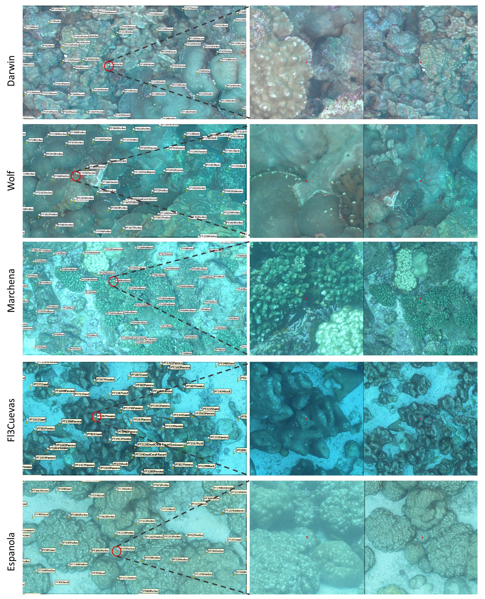
For each marker, we extract the image with the smallest reprojection error. Reprojection error is measured by projecting the point from the 3D model (origin point) to the image and back to the 3D model (target point) and calculating the distance between them. After selecting the image with minimal error, it is cropped around the point in 1600 X 1600 pixels. Eventually we resized the images by half to enable their upload resulting in 800X800 pixels per image. We also extract a novel view for each point- a synthetic image of the 3D model using a top-down projection. This image is called synthetic because it was never taken by a camera. It is a rendering of the 3D model from a given viewpoint. We used Metashape’s functions to produce these images with each marker as the center of each image and a fixed size of 1600 X 1600 pixels (Figure 3). The advantage of using both images is that the close up camera image helps to identify the class of the object while the synthetic view helps to put that in context. This is helpful for distinguishing corals such as Porites and Montipora which look similar from a close up view but have different 3D structure in the colony.
The pair of images (best camera view and synthetic image) per point was uploaded to labelbox [60], an online platform for image annotation. The camera view is a close up on the point while the synthetic image shows the 3D context of the point. Therefore, using the image pairs helps to annotate the points rapidly and accurately.
The annotations are released as part of the dataset, please see section Supp. 1.2 and Figure Supp. 2 for more details.
2.6. Classification
A total of 17,807 image pairs were annotated in 12 classes (results are detailed in Table 2): Pavona, Pocillopora, Porites, Psammocora, Rock, Sand, Tubastraea, Caulerpa, Dead Coral-Framework, Dead Coral-Rubble, Other, and Unknown. The class Dead Coral-Framework was used to describe biogenic substrate found mostly in Darwin. The class Unknown was used for points where the images (best camera view and synthetic image) did not show the same point. The class Other was used for points that were not in any category.
The images were annotated by three members of the marine monitoring team of the Charles Darwin Foundation (W.I, F.T, and W.B.S) including reviewing all image pairs to validate the classifications.
We also used a classification: "Projection quality", to describe the fit between the synthetic image and the best camera view. When both images showed the same point, we classify it as good, and when the synthetic view does not exactly align with the best camera view we classify it as bad. This can happen if the 3D point is obscured by an overhang, since the synthetic views are generated only from a top down view. We used this classification becuase in the future we aim to use these synthetic images together with the best camera view to train a neural network for coral identification, and using the synthetic views can increases the amount of training data almost twofold. Please see section Supp. 1.1 and Figure Supp. 1 for more information on using this data for training a classifier.
Figure 3.
Method for 3D annotation using the best camera and synthetic views: each row is from a different site. The left images show a 2X1 m close-up of the 3D model with the markers and their identities. The right images show the pair of images that were used to annotate a marker. For each point, two images are extracted: a 1600-pixel crop around the annotation point on the best image that depicts the point, and a novel synthetic image from a top-down view of the point.
2.7. Community Metrics
We calculated the relative abundance of each class per site by dividing the number of observations from each genus by the total number of observations in the model. We calculated the Shannon diversity only for coral classes: Pavona, Pocillopora, Porites, and Psammocora. We used R Statistical Software (v4.1.2; R Core Team 2021) and the R package vegan [61,62]. Shannon diversity is calculated as:
where is the proportion of species i, and S is the number of species.
We calculated percent coral cover calculating the proportions of four coral classes— Pavona, Pocillopora, Porites, and Psammocora, out of all classes.
We used Principal Component Analysis (PCA) to visualize the difference in community structure on two axes. We ommited the classes Unknown, Other, and Caulerpa, and from this analysis, thus reducing nine dimensions to two (Figure 5). PCA is a linear method that identifies the axes (principal components) along which the data has the greatest variance, projecting the data onto these components.
2.8. Structural Complexity Metrics
2.8.1. Fractal Dimension from Cube Counting
We previously worked on cube-counting for assessing fractal dimension of coral reefs and detailed the method extensively [37]. In short, the cube-counting method [63] enables to calculate the fractal dimension of objects as:
where is the length of the cube and N() is the number of cubes required to cover the object at a given length. N() is calculated for several cube-lengths () and the fractal dimension is calculated as the slope of the fitted line between log(N()) and log(1/).
We take each pointcloud and bound it with a minimal bounding cube ( m3). The cube is then divided into 8 equal cubes by dividing each axis. In each iteration, cubes that contain a part of the mesh are counted (Eq. 2) and used in the next iteration.
For flat shapes, the size of the cube should not affect the measurement while in complex shapes more surface detail is revealed with smaller cube sizes, and the number of cubes increase exponentially when decreasing the cube-length. flat reefs are expected to have lower values close to two, and reefs that are rich in structural features— i.e., structurally complex reefs, are expected to have values closer to three [37].
2.8.2. Fractal Dimension from Directed Geodesic Walks
This is a novel method for calculating the fractal dimension that elaborates the classic rugosity metric and applies a similar measurement over multiple scales of measurement across the full model.
We first construct a mesh from the point cloud using the Open3D Python package. The mesh is then cropped into 5 cm-wide slices with 5 cm intervals along both axes, resulting in approximately 200 slices per site. To measure the structural complexity of these slices we simulate a walk along each slice over a range of step sizes. The starting and ending points of the walk are defined as the minimal and maximal coordinates along the slice. Using PyVista [64] python package we calculate the geodesic path: the shortest path along the mesh surface—between these points. This path determines the order of points for subsequent walks therefore we call this method directed geodesic walks. We use the recorded vertices of the geodesic path as a baseline for building a new point cloud by densifying these points. This enables us to maintain the order of points rather than their coordinates for the walk algorithm.
It is crucial to balance the slice width: too wide, and the walk avoids the actual terrain, underestimating complexity; too thin, and the mesh fragments, making the walk ineffective. Moreover, we had several cases (57 out of 29,343) where the walk did not work because the algorithm was unable to find points in the specified step size. We excluded these from the FD assessment.
The algorithm follows two key rules: avoid revisiting previous points (using point indices rather than coordinates), and choose the minimal point on the axis of the walk, for example if the walk is along the x axis, choose the point with the minimal x coordinate (see Figure 4). For each slice, the walk is conducted twice per step-size : once from start to finish and then in reverse. The average number of steps is recorded, and the walk ratio is calculated as the distance traveled divided by the geodesic path length. A linear model is then fitted to the log relationship between walk ratio and step size for each slice, with the overall score per site being the mean of these measurements.
This method captures structural complexity by observing how the walk ratio decreases with increasing step size (Figure 4). For flat surfaces, step size has little effect, as both small and large steps cover similar distances. For complex surfaces, however, smaller steps traverse more intricate paths, highlighting structural complexity. This difference provides an estimate of the dimension and complexity of the reef structure. The idea is that for complex structures the walk ratio will decrease when increasing the step size. For flat surfaces, the step size r has no influence on the distance of the walk. To portray this, imagine an ant, a horse, and an elephant crossing a surface from start to end. If the surface is flat they will all travel the same distance. If the surface is wavy, rugged, and complex, the ant will travel a larger distance than the horse and elephant. Measuring how the distance traveled changes by step size gives an estimation of the dimension of the mesh and the structural complexity of the reef.
Figure 4.
Method for calculating fractal dimension from geodesic walks: A) A slice is extracted from the 3D model (left) and used to calculate the geodesic path between start and end points. This process is repeated at 5 cm intervals to extract approximately 100 slices per side (top, right). The model is then rotated 90° around the z-axis, and the process is repeated to capture slices on both axes. B) A profile of a geodesic path extracted from the 3D model. c) a close up on the slice of the mesh and the geodesic path. The geodesic path links vertices and enables us to assign the walk order by their index (ordinal) and not only their position. The algorithm works by finding points in radius (step-size) and choosing the point with the minimal coordinate on the walk axis. The bottom image in (C) shows the steps of the walk and a red circle with radius step size to illustrate how steps are chosen. the right image is a close up of the secyion outlined in dashed blue that shows step n and possible points within the radius(marked with asterisk).The chosen point n+1 is the point with minimal x coord. D) a walk ratio is determined for each step-size and used to calculate FD for the slice of the mesh. On complex paths, increase in step size causes a decrease in walk ratio. The overall score per site is the average of 200 slices (A, right).

3. Results
We studied seven reefs using 3D point annotations and structural complexity metrics. All results are summarized in Table 2:

Table 2.
Summary table of all counts, structural complexity measurements, GPS coordinates, and depth per site
Table 2.
Summary table of all counts, structural complexity measurements, GPS coordinates, and depth per site
| site name | Caulerpa | DeadCoral-Framwork | DeadCoral-Rubble | Other | Pavona | Pocillopora | Porites | Rock | Sand | Tubastraea |
|---|---|---|---|---|---|---|---|---|---|---|
| Darwin- Wellington Reef | 105 | 66 | 1 | 46 | 566 | 29 | 1108 | 855 | 177 | 9 |
| Española- Xarifa | 1 | 31 | 65 | 7 | 0 | 0 | 584 | 353 | 800 | 0 |
| Floreana- Tres Cuevitas | 0 | 11 | 12 | 12 | 731 | 1 | 0 | 1409 | 463 | 1 |
| Floreana-Punta Cormorant | 0 | 16 | 0 | 13 | 351 | 0 | 16 | 1317 | 485 | 1 |
| Marchena -Roca Espejo | 0 | 90 | 38 | 18 | 35 | 613 | 361 | 1063 | 265 | 1 |
| Pinta - Cabo Ibetson | 0 | 332 | 39 | 18 | 3 | 674 | 10 | 1423 | 64 | 0 |
| Wolf - Corales | 0 | 40 | 0 | 12 | 812 | 7 | 961 | 580 | 93 | 2 |
| Site name | Unknown | Psammocora | Cube Counting FD | mean_slope | lacunarity | SurfaceArea | Lat | Lon | Depth | |
| Darwin - Wellington Reef | 129 | 0 | 2.267 | 0.108951 | 1.495 | 309 | -91.995824 | 1.67824 | 15 | |
| Española - Xarifa | 8 | 1 | 2.138 | 0.035663 | 1.626 | 185 | -89.644622 | -1.357863 | 5 | |
| Floreana- Tres Cuevas | 130 | 8 | 2.229 | 0.101956 | 1.998 | 225 | -90.408089 | -1.236136 | 10 | |
| Floreana- Punta Cormorant | 51 | 1 | 2.202 | 0.074877 | 1.615 | 276 | -90.419325 | -1.223949 | 12 | |
| Marchena - Roca Espejo | 74 | 19 | 2.212 | 0.062882 | 1.458 | 258 | -90.401241 | 0.312162 | 8 | |
| Pinta - Cabo Ibetson | 71 | 18 | 2.208 | 0.062978 | 1.536 | 265 | -90.720945 | 0.544216 | 8 | |
| Wolf - Corales | 101 | 0 | 2.225 | 0.096196 | 1.684 | 261 | -91.815861 | 1.386624 | 12 |
3.1. Community Metrics from 3D Annotations
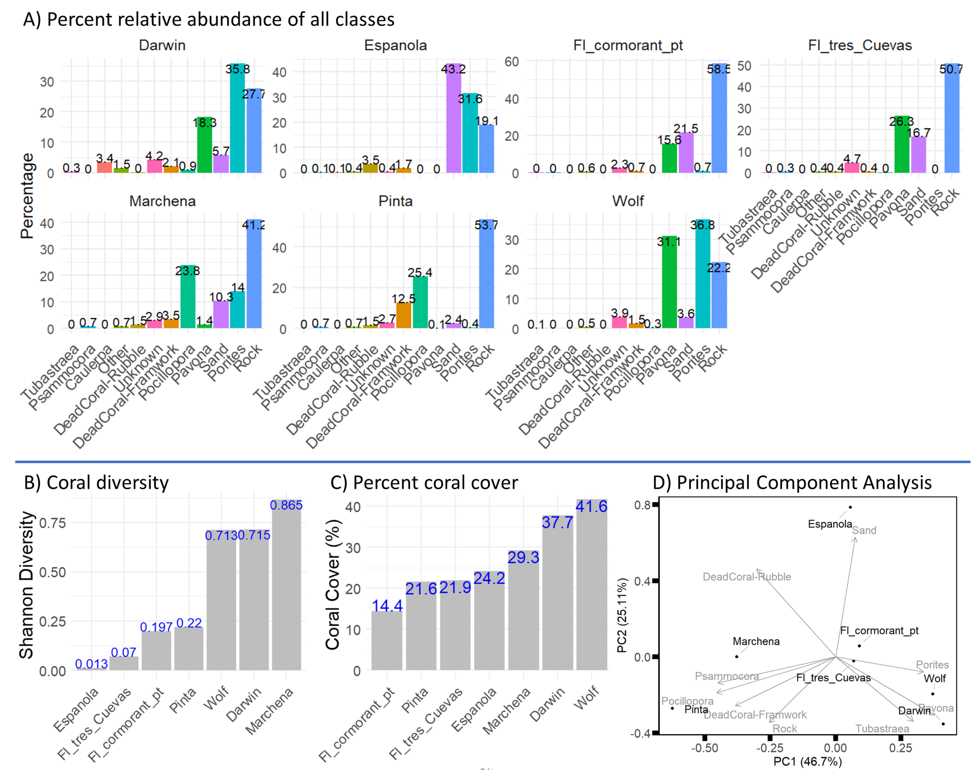
First, we examined the relative abundance of each class. The results (Figure 5, A) show that Darwin (n=3091) is dominated by Porites (36%) and Pavona (18%). Española (n = 1850) is characterized by Sand (43%) and Porites (32%). Fl_cormorant_pt (n = 2251) is dominated by rock (58%) with contributions from Sand (21%) and Pavona (15%).Fl_tres_Cuevas (n=2778) shows a high abundance of rock (51%) and Pavona (26%). Marchena (n=2577) is characterized by rock (41%) and Pocillopora (24%), with higher evenness among coral classes. Pinta (n = 2652) has substantial rock cover (54%) and Pocillopora (25%). Wolf (n=2608) is dominated by Porites (37%) and Pavona (31%).
Coral diversity (Figure 5, B) was calculated based on the coral classes Pavona, Pocillopora, Porites, and Psammocora. The results show that Marchena has the highest diversity (0.87), followed by Darwin and Wolf (0.71). Española and Fl_tres_cuevas have the lowest diversity. When examining the relative abundance of coral classes, it shows that Española is dominated by Porites, while Fl_cormorant_pt and Fl_tres_cuevas are dominated by Pavona. In contrast, Marchena, Darwin, and Wolf exhibit higher evenness among coral classes.
The results of coral cover per site (Figure 5, C) varied from 14% in Fl_cormorant_pt to 42% in Wolf. Darwin had 38% coral cover, while Fl_tres_cuevas, Pinta, and Española had 21–24%. Marchena showed 29% coral cover.
3.2. Multidimensional Scaling
We performed a Principal Component Analysis (PCA) to reduce the dimensionality of the data (Figure 5, D) and visualize site similarity and class contributions. The first and second PCs explain 49% and 25% of the variation in the data. Caulerpa and Tubastraea classes were only apparent in Darwin and Unknown and Other classes are points that were not identified and therefore we dropped them from the PCA.
The PCA biplot (Figure 5, D) shows that Darwin and Wolf are close due to their higher proportions of Porites and Pavona. Floreana sites (Fl_tres_cuevas and Fl_cormorant_pt) cluster together and are affected by Pavona, Sand, and Rock. Pinta and Marchena group together due to higher proportions of Pocillopora, and Psammocora, Española is separate from all sites due to the high proportion of Sand.
Figure 5.
A) Percent relative abundance of benthic classes across surveyed sites in the Galápagos Archipelago, highlighting site-specific trends in coral and non-coral categories. Darwin (n = 3091) is dominated by Porites and Pavona. Española (n = 1850) is characterized by Sand and Porites. Fl_cormorant_pt (n = 2251) is dominated by rock with contributions from Sand and Pavona. Fl_tres_cuevas (n = 2778) shows a high abundance of rock and Pavona. Marchena (n = 2577) is characterized by rock and Pocillopora, with higher evenness among coral classes. Pinta (n = 2652) has substantial rock cover and Pocillopora. Wolf (n = 2608) is dominated by Porites and Pavona. B) Shannon diversity index (H’) of coral genera, Marchena is the most diverse site followed by Darwin and Wolf, Española has the lowest diversity. C) Percentage of coral cover calculated as the proportion of annotations from Pavona, Pocillopora, Porites, Psammocora and Tubastraea out of all annotations, showing the highest cover in Wolf (42%) and Darwin (38%), and the lowest in Fl_cormorant_pt (14%). D) Principal Component Analysis (PCA) biplot illustrating the separation of reef sites based on their class compositions. Vectors represent the contributions of individual classes (e.g., Porites, Pavona, Pocillopora, etc.) to the variance in the data. The first and second PCs explain 49% and 25% of the variation in the data. Darwin and Wolf cluster close to one another, primarily influenced by the Porites and Pavona vectors. Floreana sites also group together, with the rock and Pavona vectors driving their composition. Pinta and Marchena are positioned further apart but are influenced by Psammocora and Pocillopora classes. Española is situated further from the other sites, with Sand contributing the most to its separation.
3.3. Structural Complexity from Cube Counting and Walk Ratios
The results of these two metrics show similar trends. To compare them we normalized them using min-max scaling and plotted them against each other (Figure 6, C). Darwin, Fl_tres_cuevas, Wolf, and Española Maintain their ranks of structural complexity in both methods. However, the sites Marchena and Pinta have the same cube counting results and slightly different walk results. Fl_cormorant_pt has higher Geodesic walk scores than these two sites, but lower FD from cube counting.
These findings emphasize the importance of using complementary metrics to understand reef structural complexity.
4. Discussion
Galápagos coral reefs have experienced severe and recurrent environmental disturbances over the past four decades, yet the extent of their resilience remains uncertain. El Niño events of 1982 and 1997 [8,11] and a La Niña event in 2007 caused cold-water upwelling and bleaching [13]. More recently, the third global bleaching event (2014–2017) led to widespread coral mortality worldwide [65], although in the Galápagos reefs displayed some resilience, potentially due to localized upwelling [66] or possible shifts in symbiont associations [11]. The fourth global bleaching event was preceded by El Niño conditions [17] and declared in March 2024 [67]. Predictions indicated that the 2024 El Niño could transition to La Niña [68] possibly adding stress to Galápagos reefs through cold-water fluxes [5]. We initiated this program in 2024 to document the corals before the El Niño and during the transition to colder water from La Niña using new technologies. Our findings provide critical new insights into the spatial variation of coral cover, diversity, and structural complexity across seven reef sites, offering a valuable baseline for future ecological assessments.
This study demonstrates the advantages of photogrammetry over traditional chain transects and planar rugosity indices, which often underestimate structural complexity by failing to capture overhangs and crevices. The high-resolution 3D models produced here not only provide greater spatial accuracy but also enable automated analyses that can be replicated across time and space, facilitating long-term coral monitoring efforts.
High structural complexity is often correlated with increased biodiversity and reef resilience, as complex habitats provide refuges for juvenile corals and associated reef organisms. Our findings suggest that reefs with high fractal dimensions, such as those at Darwin and Wolf, may serve as ecological strongholds capable of supporting diverse marine life despite environmental stressors.
Protocols for annotating photogrammetric models from underwater environments usually use the photomosaic [50,51] which is a 2D representation of the 3D model. We aimed to segment the 3D model in order to obtain samples that are obscured in the photomosaic such as from overhangs and crevices. A similar method for pointcloud annotation was previously presented [52,69] however it requires additional software. Our workflow operates in Metashape and the annotations can be distributed online, e.g., on Labelbox [60]. Moreover, using the synthetic image (the 3D model view) improves the annotation accuracy and speed because it enables to view the point in context while the close-up images facilitate precise identification. Previous research on 3D semantic segmentation of coral reef models was done via deep learning and multiview images (e.g., [54,55,56,57]). In this work, we have taken the first step toward semantic segmentation of 3D models from the region by compiling a large dataset of annotations (see section Supp. 1.1 and Supp. 1.2). An important follow up study will focus on training a deep neural net based on the image pairs presented here and testing if the novel views increase the accuracy in predicting benthic classes.
Our results reveal significant variation in coral cover and diversity across sites. Northern sites, such as Darwin and Wolf, exhibited the highest coral cover, primarily dominated by Porites and Pavona species. In contrast, Marchena demonstrated the highest species diversity, with more even representation among Pavona, Pocillopora, Psammocora, and Porites. Floreana sites had relatively lower coral cover but exhibited high structural complexity, suggesting that these reefs may still provide essential habitat for reef-associated organisms despite their lower coral abundance. These patterns suggest that both geographical location and depth significantly influence coral community composition, although this was not directly tested. Our findings align with previous research, which documented higher coral cover in northern sites and patchier distributions in central and southern locations. However, our study expands upon prior work by incorporating 3D structural complexity assessments, which provide a more comprehensive understanding of reef habitat variation.
Previous studies in the region showed that coral cover is highest at the northern sites and that diversity however was highest at Marchena to the south. Coral cover at Darwin was quantified very close to our site using 0.25 m2 photo quadrats sampling 37.5 m2 per site (15 transects × 10 photos × 0.25 m2) [70]. The authors reported a total coral cover of 21.1%, with Porites contributing 19.5%, and Pavona and Pocillopora spp. each contributing less than 0.4%. By comparison, we sampled a 100 m2 area at Darwin and found 41.7% coral cover, with Porites contributing 35.8%, Pavona 18.4%, and Pocillopora 1%.
Point-intercept methods along several 100 m transects per site at Wolf, Darwin, and Marchena were previously conducted [13]. At Wolf (Bahía Tiburón B), the authors reported 48% live coral, 25% rock, and 5% sand, with Porites and Pavona as the most abundant corals. For comparison, we found 42% coral cover, also dominated by Porites and Pavona. At Darwin (Anchorage Point 4), they observed 53% live coral, 37% dead coral, and 11% sand, with Porites and Pavona as the dominant genera. Our results were similar, with 38% coral cover dominated by Porites and Pavona. At Marchena, they noted high diversity and recorded 7% live coral, 34% rock, and 25% sand, with Porites, Pavona, and Pocillopora as the most abundant genera. In comparison, we found 29% live cover, dominated by Pocillopora and Porites. Moreover, we found that Fl_tres_cuevas had low coral cover and diversity but exhibited high structural metrics suggesting that it provides a rich habitat for reef organisms via diverse structural features.
Calculating fractal dimension from geodesic walks is a novel method developed for analyzing wide-scale reef models. Cube counting for fractal dimension was implemented by us previously on smaller models [37], however, it’s less effective for large area models because of their extensive lateral extent and relatively shallow vertical features, which result in larger cube sizes being mostly empty. In Figure 6, A and B appear different primarily due to the range on the y-axis. Since cube counting operates in 3D space its slope is steeper compared to walk ratios which operate in 1D. Darwin, Fl_tres_cuevas, and Wolf exhibit the highest fractal dimension from box counting and geodesic walks. Española has the lowest slope, suggesting a more flat reef structure. Geodesic walks enable to depict structural complexity in large area models effectively. This is evident in the results (Figure 6c) where geodesic walks maintain similar rank orderings among sites as cube counting. Nevertheless, there are some discrepancies, most notably between Pinta/Marchena and Fl_cormorant_pt. Here, cube counting overestimates structural complexity. The first two are relatively flat models abundant in Pocillopora. On the other hand, Fl_cormorant_pt has an abundance of Pavonas colonies scattered across the substrate in different sizes (Figure 2). Cube counting rated these sites high probably because of differences in the small box sizes.
Our application of novel photogrammetric techniques represents a significant methodological advancement in Galápagos coral research. Traditional reef complexity measurements, such as chain transects and planar rugosity indices, often fail to capture the full three-dimensionality of reef structures, especially overhangs and crevices where cryptic species reside. By implementing fractal dimension analysis through directed geodesic walks, we introduce a refined approach that better quantifies fine-scale reef complexity across multiple spatial scales. This method enhances our ability to compare reefs with different structural compositions and provides a robust metric for monitoring long-term changes in habitat complexity. We release a new dataset: Galápagos_3D, including the 3D models used in this study together with 3D annotations and classified image pairs. This data is useful for studies in ecology and computer graphics such as 3D segmentation from sparse labels via region growing [71].
While our study provides a valuable baseline, several limitations should be considered. First, although photogrammetry allows for detailed 3D modeling, manual annotation of benthic classes remains labor-intensive. Future research should explore machine-learning approaches to automate annotation, potentially improving efficiency and scalability. Additionally, while we documented spatial variation in reef complexity, temporal monitoring is needed to assess long-term resilience. Repeated surveys, particularly following extreme climatic events, will be crucial in understanding whether certain coral communities are developing adaptive responses to recurring stressors.
Given the increasing frequency of marine heatwaves and El Niño events, understanding which coral communities are most resilient and why will be critical for conservation planning. Our findings suggest that structural complexity may play a key role in reef persistence by providing refuges for coral recruits and associated marine life. Conservation efforts should prioritize sites with high coral cover and structural heterogeneity, as these areas may serve as ecological strongholds in the face of climate change.
Future studies should focus on longitudinal assessments, combining photogrammetry with genetic and physiological analyses to identify potential resilience mechanisms in Galápagos corals. Additionally, integrating satellite remote sensing data with underwater photogrammetry could enhance large-scale monitoring efforts, providing a more comprehensive picture of coral ecosystem health. In conclusion, this study highlights the importance of high-resolution 3D mapping for understanding coral reef dynamics and sets a new standard for reef monitoring in the Galápagos. By continuing this long-term research effort, we can contribute to evidence-based conservation policies, ensuring the preservation of these ecologically vital ecosystems for future generations.
- The authors used chatGPT and the Metashape online forum to generate the code and figures in the mansucript.
Supplementary Materials
The following supporting information can be downloaded at the website of this paper posted on Preprints.org.
Author Contributions
Methodology, software, formal analysis, investigation, data curation, writing—original draft preparation, visualization: M.Y.; Conceptualization, resources, project administration, writing—review and editing: M.Y., W.B.S., I.K.; image annotation and validation, fieldwork assistance: F.T., W.B.S., W.I.; supervision, funding acquisition: I.K.; All authors have read and agreed to the published version of the manuscript.
Funding
Research funding was provided by the Mark and Rachael Rohr Foundation, Ocean Finance Company, the Paul M. Angell Family Foundation, Lindland, National Geographic, and Ken Collins and Jennifer Mallinson.
Data Availability Statement
The Galápagos_3D dataset including 3D point clouds, image pairs, and annotations will be made available on Zenodo. The code is for structural complexity analysis is available at https://github.com/MatanYuval/Galapagos-Community-structure.
Acknowledgments
We thank Johny Mason of the Charles Darwin Foundation for his excellent work on the map in Figure 1. All authors gratefully acknowledge the Galapagos National Park for authorizing this investigation (research permit: PC-31-24). This publication is contribution number 2711 of the Charles Darwin Foundation for the Galapagos Islands.
Conflicts of Interest
The authors declare no conflicts of interest.
Abbreviations
The following abbreviations are used in this manuscript:
| Principal Component Analysis | PCA |
| Fractal Dimension | FD |
References
- Izurieta, A.; Delgado, B.; Moity, N.; Calvopina, M.; Cedeno, Y.; Banda-Cruz, G.; Cruz, E.; Aguas, M.; Arroba, F.; Astudillo, I.; et al. A collaboratively derived environmental research agenda for Galápagos. Pacific Conservation Biology 2018, 24, 207. [Google Scholar]
- Glynn, P.W.; Wellington, G.M. Corals and coral reefs of the Galápagos Islands; Univ of California Press, 1983.
- Riegl, B.; Johnston, M.; Glynn, P.W.; Keith, I.; Rivera, F.; Vera-Zambrano, M.; Banks, S.; Feingold, J.; Glynn, P.J. Some environmental and biological determinants of coral richness, resilience and reef building in Galápagos (Ecuador). Scientific Reports 2019, 9, 10322. [Google Scholar]
- Dawson, T.; Henderson, S.; Banks, S. Galapagos coral conservation: impact mitigation, mapping and monitoring. Galapagos Res 2009, 66, 65–74. [Google Scholar]
- Foreman, A.D.; Duprey, N.N.; Yuval, M.; Dumestre, M.; Leichliter, J.N.; Rohr, M.C.; Dodwell, R.C.; Dodwell, G.A.; Clua, E.E.; Treibitz, T.; et al. Severe cold-water bleaching of a deep-water reef underscores future challenges for Mesophotic Coral Ecosystems. Science of the Total Environment 2024, 951, 175210. [Google Scholar] [CrossRef] [PubMed]
- Hickman Jr, C.P. Evolutionary responses of marine invertebrates to insular isolation in Galapagos. Galapagos Research 2009. [Google Scholar]
- Edgar, G.J.; Banks, S.A.; Brandt, M.; Bustamante, R.H.; Chiriboga, A.; Earle, S.A.; Garske, L.E.; Glynn, P.W.; Grove, J.S.; Henderson, S.; et al. El Niño, grazers and fisheries interact to greatly elevate extinction risk for Galapagos marine species. Global Change Biology 2010, 16, 2876–2890. [Google Scholar] [CrossRef]
- Glynn, P.W.; Feingold, J.S.; Baker, A.; Banks, S.; Baums, I.B.; Cole, J.; Colgan, M.W.; Fong, P.; Glynn, P.J.; Keith, I.; et al. State of corals and coral reefs of the Galápagos Islands (Ecuador): Past, present and future. Marine Pollution Bulletin 2018, 133, 717–733. [Google Scholar]
- Glynn, P.W.; Riegl, B.; Purkis, S.; Kerr, J.M.; Smith, T.B. Coral reef recovery in the Galápagos Islands: the northernmost islands (Darwin and Wenman). Coral Reefs 2015, 34, 421–436. [Google Scholar] [CrossRef]
- Keith, I.; Dawson, T.P.; Collins, K.J.; Campbell, M.L. Marine invasive species: establishing pathways, their presence and potential threats in the Galapagos Marine Reserve. Pacific Conservation Biology 2016, 22, 377–385. [Google Scholar]
- Feingold, J.S.; Glynn, P.W. Coral research in the Galápagos Islands, Ecuador. In The Galápagos marine reserve: a dynamic social-ecological system; Springer, 2013; pp. 3–22.
- Glynn, P.W. State of coral reefs in the Galápagos Islands: natural vs anthropogenic impacts. Marine Pollution Bulletin 1994, 29, 131–140. [Google Scholar]
- Banks, S.; Vera, M.; Chiriboga, A. Establishing reference points to assess long-term change in zooxanthellate coral communities of the northern Galápagos coral reefs. Galapagos Research 2009. [Google Scholar]
- Glynn, P.J.; Glynn, P.W.; Riegl, B. El Niño, echinoid bioerosion and recovery potential of an isolated Galápagos coral reef: a modeling perspective. Marine Biology 2017, 164, 1–17. [Google Scholar]
- Rhoades, O.K.; Brandt, M.; Witman, J.D. La Niña-related coral death triggers biodiversity loss of associated communities in the Galápagos. Marine Ecology 2023, 44, e12767. [Google Scholar]
- Peñaherrera-Palma, C.; Harpp, K.; Banks, S. Rapid seafloor mapping of the northern Galapagos Islands, Darwin and Wolf. Galapagos Research 2016. [Google Scholar]
- López-Pérez, A.; Granja-Fernández, R.; Ramírez-Chávez, E.; Valencia-Méndez, O.; Rodríguez-Zaragoza, F.A.; González-Mendoza, T.; Martínez-Castro, A. Widespread Coral Bleaching and Mass Mortality of Reef-Building Corals in Southern Mexican Pacific Reefs Due to 2023 El Niño Warming. In Proceedings of the Oceans. MDPI. 2024; 5, 196–209. [Google Scholar]
- Burns, J.; Delparte, D.; Gates, R.; Takabayashi, M. Integrating structure-from-motion photogrammetry with geospatial software as a novel technique for quantifying 3D ecological characteristics of coral reefs. PeerJ 2015, 3, e1077. [Google Scholar]
- Ferrari, R.; Figueira, W.F.; Pratchett, M.S.; Boube, T.; Adam, A.; Kobelkowsky-Vidrio, T.; Doo, S.S.; Atwood, T.B.; Byrne, M. 3D photogrammetry quantifies growth and external erosion of individual coral colonies and skeletons. Scientific Reports 2017, 7, 16737. [Google Scholar]
- Yuval, M.; Alonso, I.; Eyal, G.; Tchernov, D.; Loya, Y.; Murillo, A.C.; Treibitz, T. Repeatable semantic reef-mapping through photogrammetry and label-augmentation. Remote Sensing 2021, 13, 659. [Google Scholar]
- Risk, M.J. Fish diversity on a coral reef in the Virgin Islands. Atoll research bulletin 1972. [Google Scholar]
- Loya, Y. Plotless and transect methods. Coral reefs: research methods. UNESCO, Paris 1978, pp. 197–217.
- Hill, J.; Wilkinson, C. Methods for ecological monitoring of coral reefs. Australian Institute of Marine Science, Townsville 2004, 117. [Google Scholar]
- Laxton, J.; Stablum, W. Sample design for quantitative estimation of sedentary organisms of coral reefs. Biological Journal of the Linnean Society 1974, 6, 1–18. [Google Scholar]
- Ott, B. Community patterns on a submerged barrier reef at Barbados, West Indies. Internationale Revue der gesamten Hydrobiologie und Hydrographie 1975, 60, 719–736. [Google Scholar]
- Remmers, T.; Grech, A.; Roelfsema, C.; Gordon, S.; Lechene, M.; Ferrari, R. Close-range underwater photogrammetry for coral reef ecology: a systematic literature review. Coral Reefs 2024, 43, 35–52. [Google Scholar]
- Luckhurst, B.; Luckhurst, K. Analysis of the influence of substrate variables on coral reef fish communities. Marine Biology 1978, 49, 317–323. [Google Scholar]
- Rogers, C.S.; Garrison, G.; Grober, R.; Hillis, Z.M.; Franke, M.A. Coral Reef Monitoring Manual for the Caribbean and Western Atlantic. Technical report, Virgin Islands National Park., 1994.
- Rogers, C.S.; Miller, J. Coral bleaching, hurricane damage, and benthic cover on coral reefs in St. John, US Virgin Islands: a comparison of surveys with the chain transect method and videography. Bulletin of Marine Science 2001, 69, 459–470. [Google Scholar]
- Knudby, A.; LeDrew, E. Measuring Structural Complexity on Coral Reefs. Proceedings of the American Academy of Underwater Sciences 26th Symposium, 2007; 181–188. [Google Scholar]
- Bryson, M.; Ferrari, R.; Figueira, W.; Pizarro, O.; Madin, J.; Williams, S.; Byrne, M. Characterization of measurement errors using structure-from-motion and photogrammetry to measure marine habitat structural complexity. Ecology and Evolution 2017, 7, 5669–5681. [Google Scholar] [PubMed]
- Friedman, A.; Pizarro, O.; Williams, S.B.; Johnson-Roberson, M. Multi-scale measures of rugosity, slope and aspect from benthic stereo image reconstructions. PloS one 2012, 7, e50440. [Google Scholar]
- Ferrari, R.; McKinnon, D.; He, H.; Smith, R.N.; Corke, P.; González-Rivero, M.; Mumby, P.J.; Upcroft, B. Quantifying multiscale habitat structural complexity: a cost-effective framework for underwater 3D modelling. Remote Sensing 2016, 8, 113. [Google Scholar]
- González-Rivero, M.; Harborne, A.R.; Herrera-Reveles, A.; Bozec, Y.M.; Rogers, A.; Friedman, A.; Ganase, A.; Hoegh-Guldberg, O. Linking fishes to multiple metrics of coral reef structural complexity using three-dimensional technology. Scientific Reports 2017, 7, 13965. [Google Scholar]
- Hylkema, A.; Debrot, A.O.; Osinga, R.; Bron, P.S.; Heesink, D.B.; Izioka, A.K.; Reid, C.B.; Rippen, J.C.; Treibitz, T.; Yuval, M.; et al. Fish assemblages of three common artificial reef designs during early colonization. Ecological Engineering 2020, 157, 105994. [Google Scholar]
- Urbina-Barreto, I.; Chiroleu, F.; Pinel, R.; Fréchon, L.; Mahamadaly, V.; Elise, S.; Kulbicki, M.; Quod, J.P.; Dutrieux, E.; Garnier, R.; et al. Quantifying the shelter capacity of coral reefs using photogrammetric 3D modeling: From colonies to reefscapes. Ecological Indicators 2021, 121, 107151. [Google Scholar]
- Yuval, M.; Pearl, N.; Tchernov, D.; Martinez, S.; Loya, Y.; Bar-Massada, A.; Treibitz, T. Assessment of storm impact on coral reef structural complexity. Science of The Total Environment 2023, 891, 164493. [Google Scholar] [CrossRef] [PubMed]
- Aston, E.A.; Duce, S.; Hoey, A.S.; Ferrari, R. A Protocol for Extracting Structural Metrics From 3D Reconstructions of Corals. Frontiers in Marine Science 2022, 9, 854395. [Google Scholar] [CrossRef]
- Mandelbrot, B.B.; Passoja, D.E.; Paullay, A.J. Fractal character of fracture surfaces of metals. Nature 1984, 308, 721–722. [Google Scholar] [CrossRef]
- Nash, K.L.; Graham, N.A.; Wilson, S.K.; Bellwood, D.R. Cross-scale habitat structure drives fish body size distributions on coral reefs. Ecosystems 2013, 16, 478–490. [Google Scholar] [CrossRef]
- Reichert, J.; Backes, A.R.; Schubert, P.; Wilke, T. The power of 3D fractal dimensions for comparative shape and structural complexity analyses of irregularly shaped organisms. Methods in Ecology and Evolution 2017, 8, 1650–1658. [Google Scholar]
- Fukunaga, A.; Burns, J.H. Metrics of coral reef structural complexity extracted from 3D mesh models and digital elevation models. Remote Sensing 2020, 12, 2676. [Google Scholar]
- Torres-Pulliza, D.; Dornelas, M.A.; Pizarro, O.; Bewley, M.; Blowes, S.A.; Boutros, N.; Brambilla, V.; Chase, T.J.; Frank, G.; Friedman, A.; et al. A geometric basis for surface habitat complexity and biodiversity. Nature Ecology & Evolution 2020, 4, 1495–1501. [Google Scholar]
- Miller, S.; Yadav, S.; Madin, J.S. The contribution of corals to reef structural complexity in Kāne ‘ohe Bay. Coral Reefs 2021, 40, 1679–1685. [Google Scholar] [CrossRef]
- McCarthy, O.S.; Smith, J.E.; Petrovic, V.; Sandin, S.A. Identifying the drivers of structural complexity on Hawaiian coral reefs. Marine Ecology Progress Series 2022, 702, 71–86. [Google Scholar] [CrossRef]
- Kornder, N.A.; Cappelletto, J.; Mueller, B.; Zalm, M.J.; Martinez, S.J.; Vermeij, M.J.; Huisman, J.; de Goeij, J.M. Implications of 2D versus 3D surveys to measure the abundance and composition of benthic coral reef communities. Coral Reefs 2021, 40, 1137–1153. [Google Scholar] [CrossRef]
- Loya, Y. Community structure and species diversity of hermatypic corals at Eilat, Red Sea. Marine Biology 1972, 13, 100–123. [Google Scholar] [CrossRef]
- Ferrari, R.; Lachs, L.; Pygas, D.R.; Humanes, A.; Sommer, B.; Figueira, W.F.; Edwards, A.J.; Bythell, J.C.; Guest, J.R. Photogrammetry as a tool to improve ecosystem restoration. Trends in Ecology & Evolution 2021, 36, 1093–1101. [Google Scholar]
- Pavoni, G.; Corsini, M.; Callieri, M.; Palma, M.; Scopigno, R. SEMANTIC SEGMENTATION OF BENTHIC COMMUNITIES FROM ORTHO-MOSAIC MAPS. International Archives of the Photogrammetry, Remote Sensing & Spatial Information Sciences, 2019. [Google Scholar]
- Pavoni, G.; Corsini, M.; Ponchio, F.; Muntoni, A.; Edwards, C.; Pedersen, N.; Sandin, S.; Cignoni, P. TagLab: AI-assisted annotation for the fast and accurate semantic segmentation of coral reef orthoimages. Journal of field robotics 2022, 39, 246–262. [Google Scholar]
- Remmers, T.; Boutros, N.; Wyatt, M.; Gordon, S.; Toor, M.; Roelfsema, C.; Fabricius, K.; Grech, A.; Lechene, M.; Ferrari, R. RapidBenthos: Automated segmentation and multi-view classification of coral reef communities from photogrammetric reconstruction. Methods in Ecology and Evolution 2024. [Google Scholar]
- Petrovic, V.; Vanoni, D.J.; Richter, A.M.; Levy, T.E.; Kuester, F. Visualizing high resolution three-dimensional and two-dimensional data of cultural heritage sites. Mediterranean Archaeology and Archaeometry 2014, 14, 93–100. [Google Scholar]
- Pavoni, G.; Pierce, J.; Edwards, C.B.; Corsini, M.; Petrovic, V.; Cignoni, P. Integrating Widespread Coral Reef Monitoring Tools for Managing both Area and Point Annotations. The International Archives of the Photogrammetry, Remote Sensing and Spatial Information Sciences 2024, 48, 327–333. [Google Scholar]
- King, A.; M Bhandarkar, S.; Hopkinson, B.M. Deep Learning for Semantic Segmentation of Coral Reef Images Using Multi-View Information. In Proceedings of the Proceedings of the IEEE Conference on Computer Vision and Pattern Recognition Workshops, 2019, pp. 1–10.
- Pierce, J.; Butler IV, M.J.; Rzhanov, Y.; Lowell, K.; Dijkstra, J.A. Classifying 3-D models of coral reefs using structure-from-motion and multi-view semantic segmentation. Frontiers in Marine Science 2021, 8, 706674. [Google Scholar]
- Marlow, J.; Halpin, J.E.; Wilding, T.A. 3D photogrammetry and deep-learning deliver accurate estimates of epibenthic biomass. Methods in Ecology and Evolution 2024, 15, 965–977. [Google Scholar] [CrossRef]
- Sauder, J.; Banc-Prandi, G.; Meibom, A.; Tuia, D. Scalable semantic 3D mapping of coral reefs with deep learning. Methods in Ecology and Evolution 2024, 15, 916–934. [Google Scholar] [CrossRef]
- Vera, M.; Banks, S. Health status of the coral communities of the northern Galapagos Islands Darwin, Wolf and Marchena. Galapagos Res 2009, 66, 3–5. [Google Scholar]
- Zhou, Q.Y.; Park, J.; Koltun, V. Open3D: A Modern Library for 3D Data Processing. arXiv:1801.09847, 2018; arXiv:1801.09847. [Google Scholar]
- Labelbox. Online, 2025.
- R Core Team. R: A Language and Environment for Statistical Computing. R Foundation for Statistical Computing, Vienna, Austria. 2021.
- Oksanen, J.; Simpson, G.L.; Blanchet, F.G.; Kindt, R.; Legendre, P.; Minchin, P.R.; O’Hara, R.; Solymos, P.; Stevens, M.H.H.; Szoecs, E.; et al. vegan: Community Ecology Package, 2024. R package version 2.6-8.
- Schroeder, M. Fractals, Chaos, Power Laws: Minutes from an infinite paradise, 1991.
- Sullivan, C.B.; Kaszynski, A. PyVista: 3D plotting and mesh analysis through a streamlined interface for the Visualization Toolkit (VTK). Journal of Open Source Software 2019, 4, 1450. [Google Scholar] [CrossRef]
- Eakin, C.M.; Sweatman, H.P.; Brainard, R.E. The 2014–2017 global-scale coral bleaching event: insights and impacts. Coral Reefs 2019, 38, 539–545. [Google Scholar]
- Riegl, B.; Glynn, P.W.; Banks, S.; Keith, I.; Rivera, F.; Vera-Zambrano, M.; D’Angelo, C.; Wiedenmann, J. Heat attenuation and nutrient delivery by localized upwelling avoided coral bleaching mortality in northern Galapagos during 2015/2016 ENSO. Coral Reefs 2019, 38, 773–785. [Google Scholar]
- Reimer, J.D.; Peixoto, R.S.; Davies, S.W.; Traylor-Knowles, N.; Short, M.L.; Cabral-Tena, R.A.; Burt, J.A.; Pessoa, I.; Banaszak, A.T.; Winters, R.S.; et al. The Fourth Global Coral Bleaching Event: Where do we go from here? Coral Reefs 2024, pp. 1–5.
- NOAA. ENSO Diagnostic Discussion, 2024. Retrieved December 29, 2024.
- Fox, M.D.; Carter, A.L.; Edwards, C.B.; Takeshita, Y.; Johnson, M.D.; Petrovic, V.; Amir, C.G.; Sala, E.; Sandin, S.A.; Smith, J.E. Limited coral mortality following acute thermal stress and widespread bleaching on Palmyra Atoll, central Pacific. Coral Reefs 2019, 38, 701–712. [Google Scholar]
- Glynn, P.W.; Riegl, B.; Correa, A.; Baums, I.B. Rapid recovery of a coral reef at Darwin Island, Galapagos Islands. Galapagos Research 2009, 66, 6. [Google Scholar]
- Zhan, Q.; Liang, Y.; Xiao, Y. Color-based segmentation of point clouds. Laser scanning 2009, 38, 155–161. [Google Scholar]
Figure 1.
Overview of the Galápagos Archipelago and study sites: Map of the Galápagos Archipelago with the study sites shown in red triangles within the marine reserve (outer line). The Galápagos Archipelago lies on the equator in the Eastern Tropical Pacific approx. 1000 km off the coast of Ecuador.
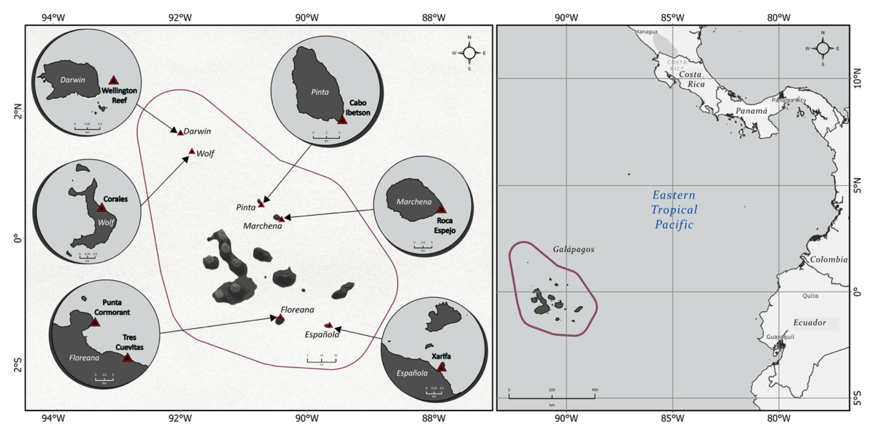
Figure 2.
The 3D models from Darwin, Wolf, Marchena, Pinta, Floreana, and Española: each image shows the 3D model of a site. The models are . A grid is shown in the background of each model.
Figure 2.
The 3D models from Darwin, Wolf, Marchena, Pinta, Floreana, and Española: each image shows the 3D model of a site. The models are . A grid is shown in the background of each model.
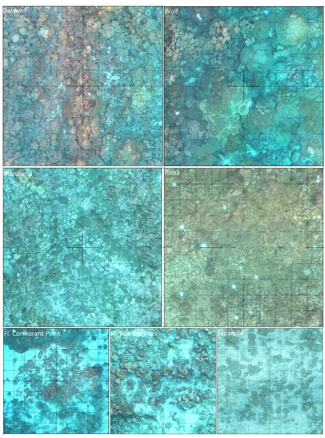
Figure 6.
Relationships between structural complexity methods: (A) Linear fit of log(Number of Cubes) vs. log(1 / Side Length), showing slopes for each site. The slopes represent fractal dimensions estimated through cube counting, with values ranging from 2.138 in Española to 2.267 in Darwin. (B) Linear fit of log(Walk Ratio) vs. log(1 / Step Size) was calculated for each slice of the mesh, we then calculated the average slope for each site (shown in legend). The slopes represent the Fractal dimension from geodesic walk ratios, ranging from 0.040 in Española to 0.122 in Darwin. (C) Cube Counting Fractal Dimensions (FD) plotted against Geodesic Walk Slopes. The data was normalized between 0-1, and the order of the sites is mostly conserved illustrating a strong correlation.
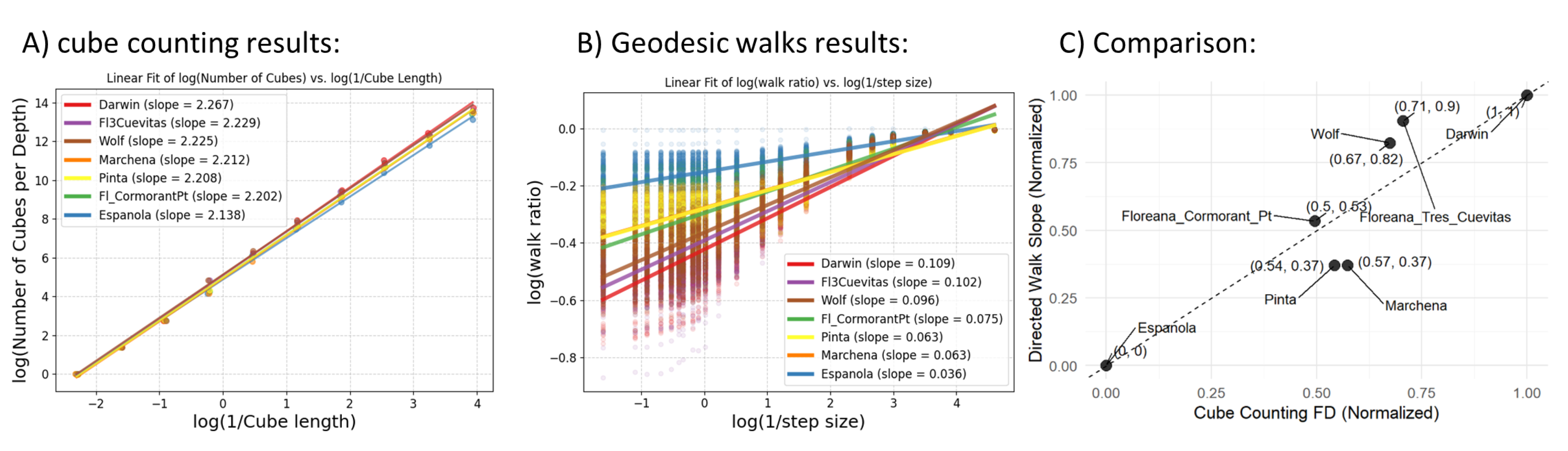
Table 1.
3D Processing Parameters in Metashape software
| Alignment Parameters | Values |
|---|---|
| Accuracy | High |
| Generic preselection | Yes |
| Reference preselection | No |
| Key point limit | 40,000 |
| Key point limit per Mpx | 1,000 |
| Tie point limit | 4,000 |
| Exclude stationary tie points | Yes |
| Guided image matching | No |
| Adaptive camera model fitting | Yes |
| Depth Maps Generation Parameters | Values |
| Quality | High |
| Filtering mode | Mild |
| Reconstruction Parameters | Values |
| Surface type | Arbitrary |
| Source data | Depth maps |
| Interpolation | Enabled |
Disclaimer/Publisher’s Note: The statements, opinions and data contained in all publications are solely those of the individual author(s) and contributor(s) and not of MDPI and/or the editor(s). MDPI and/or the editor(s) disclaim responsibility for any injury to people or property resulting from any ideas, methods, instructions or products referred to in the content. |
© 2025 by the authors. Licensee MDPI, Basel, Switzerland. This article is an open access article distributed under the terms and conditions of the Creative Commons Attribution (CC BY) license (http://creativecommons.org/licenses/by/4.0/).
Copyright: This open access article is published under a Creative Commons CC BY 4.0 license, which permit the free download, distribution, and reuse, provided that the author and preprint are cited in any reuse.


