
Submitted:
31 March 2025
Posted:
31 March 2025
You are already at the latest version
Abstract
The increasing adoption of deep neural networks (DNNs) in critical domains such as healthcare, finance, and autonomous systems underscores the growing importance of explainable artificial intelligence (XAI). In these high-stakes applications, understanding the decision-making processes of models is essential for ensuring trust and safety. However, traditional DNNs often function as "black boxes," delivering accurate predictions without providing insight into the factors driving their outputs. Expected Gradients (EG) is a prominent method for making such explanations by calculating the contribution of each input feature to the final decision. Despite its effectiveness, conventional baselines used in state-of-the-art implementations of EG often lack a clear definition of what constitutes "missing" information. In this work, we propose DeepPrior-EG, a deep prior-guided EG framework for leveraging prior knowledge to more accurately align with the concept of missingness and enhance interpretive fidelity. It resolves the baseline misalignment by initiating gradient path integration from learned prior baselines, which derived from the deep features of CNN layers. This approach not only mitigates feature absence artifacts but also amplifies critical feature contributions through adaptive gradient aggregation. We further introduce two probabilistic prior modeling strategies: a multivariate Gaussian model (MGM) to capture high-dimensional feature interdependencies and a Bayesian nonparametric Gaussian mixture model (BGMM) that autonomously infers mixture complexity for heterogeneous feature distributions. We also develop an explanation-driven model retraining paradigm to valid the robustness of the proposed framework. Comprehensive evaluations across various qualitative and quantitative metrics demonstrate the its superior interpretability. The BGMM variant achieves state-of-the-art performance in attribution quality and faithfulness against existing methods. DeepPrior-EG advances the interpretability of complex models within the XAI landscape and unlocks its potential in safety-critical applications.
Keywords:
explainable AI
; expected gradients
; prior baseline
; feature attributions
1. Introduction
The rapid advancement of Artificial Intelligence (AI) technologies has profoundly transformed a wide range of fields, including natural sciences, medicine, and engineering [1,2,3]. In these domains, AI has not only improved the efficiency of data analysis but also optimized experimental processes and design workflows. However, as deep neural networks (DNNs) achieve remarkable success in areas such as computer vision, their "black-box" nature has become increasingly apparent. This lack of transparency in decision-making processes raises significant concerns about trust and safety in critical applications such as medical diagnostics, financial decision-making, and autonomous driving [4]. Consequently, enhancing model interpretability has emerged as a crucial research objective [5,6].
Explainable AI (XAI) addresses this challenge by developing models that provide not only accurate predictions but also transparent explanations of their decision-making processes, thereby improving reliability and enabling users to better understand their internal mechanisms [7]. XAI methods are generally categorized into two main types: intrinsically interpretable models and post-hoc explanation techniques [8,9]. Intrinsically interpretable models, such as decision trees, linear regression, and logistic regression, generate predictions based on clear rules or linear relationships, making them inherently traceable and interpretable [10,11,12]. However, these models are often limited in their ability to handle high-dimensional data and complex nonlinear relationships [13,14,15]. As a result, for complex models like DNNs, post-hoc explanation methods have become the dominant approach.
Among post-hoc explanation methods, feature attribution techniques have emerged as essential tools for interpreting the behavior of DNNs [16]. These methods aim to reveal the influence of input features on model predictions, providing insights into how decisions are made. For example, interpretable deep learning models have been shown to assist medical professionals in understanding prediction rationales, ultimately improving decision-making in clinical settings [17,18,19,20].
Gradient-based attribution methods are among the most widely used approaches in feature attribution. Integrated gradients, a prominent technique within this category, quantify the contribution of each input feature by integrating gradients along the path from a baseline to the input [21]. This method addresses key limitations of earlier gradient-based approaches, particularly regarding sensitivity and implementation invariance. For instance, the sensitivity axiom ensures that a feature’s significant influence is reflected in the attribution results, while implementation invariance guarantees consistent attributions for functionally equivalent neural networks [22]. In contrast, methods like DeepLIFT [18] and Layer-wise Relevance Propagation [19], which rely on discrete gradients, fail to satisfy these axioms. Expected gradients extend integrated gradients by using the dataset expectation as a baseline, reducing dependency on a single baseline and addressing the "blindness" issue inherent in integrated gradients [23]. This approach provides smoother interpretations and greater robustness to noise.
In both integrated gradients and expected gradients, the baseline plays a critical role as a hyperparameter, representing the starting point for simulating feature "missingness" [17]. From a game-theoretic perspective, the contribution of participants is measured by incremental changes, analogous to evaluating feature importance by assessing the impact of transitioning from "missing" to "present" on model output. In practice, selecting an appropriate baseline in integrated gradients can be challenging. For example, in medical datasets, setting a blood glucose value of zero to represent missingness is inappropriate, as low blood glucose itself may indicate a hazardous condition. Similarly, in image data, a zero baseline can lead to "blindness" in scenarios where pixels identical to the baseline color (e.g., black pixels) fail to be distinguished. Expected gradients mitigate this issue by sampling multiple baselines from a distribution and averaging them, resulting in smoother and more robust explanations. Nevertheless, questions remain about whether the average of these baselines truly represents feature missingness.
To address these challenges, we propose incorporating prior knowledge into baselines to better align them with the concept of missingness. Prior information is widely used in traditional tasks such as image segmentation, where it often includes appearance priors and shape priors. For instance, appearance priors leverage distributions of intensity, color, or texture characteristics in target objects to construct segmentation models that match expected appearances, often modeled using Multivariate Gaussian Models. Shape priors, on the other hand, utilize typical geometric shapes of objects, such as organ structures, to guide segmentation boundaries [24]. While priors are extensively applied in computer vision, their integration into interpretability methods remains limited. Existing methods that incorporate priors, such as BayLIME [25], introduce prior knowledge during linear model training, which is unsuitable for addressing baseline alignment issues in gradient-based attribution methods.
This study introduces a framework for expected gradient explanations that incorporates a novel prior-based baseline. The core concept of expected gradients is to quantify the contribution of each input feature to the final decision by integrating gradients along the path from the baseline to the input image x, and then taking the expectation. However, traditional baselines in expected gradients often fail to effectively align with the concept of missingness, potentially introducing interpretive bias. To address this limitation, we propose using a prior baseline defined as , which incorporates prior information to enable a more precise representation of "missing." Unlike conventional baselines, which serve as simple statistical measures of the original data, our prior baseline acts as a flexible reference point that emphasizes prior information, enhancing interpretive fidelity by accurately reflecting feature absence. By subtracting a probability distribution, we create a neutral and objective reference that strengthens the capacity of expected gradients to reveal feature contributions, particularly those distinguishing objects from their background.
The primary contributions of this paper are as follows.
- We propose DeepPrior-EG, a deep prior-guided EG framework for addressing the longstanding issue of misalignment between baselines and the concept of missingness. It strategically initiates gradient path integration from the prior baselines, computing expectation gradients along the trajectory spanning to the input image. It autonomously also extracts priors from the intrinsic deep features of the CNN layers.
- We achieve these priors through two strategies: a multivariate Gaussian model (MGM) formulation that captures high-dimensional feature interdependencies, and a Bayesian nonparametric Gaussian mixture model(BGMM) approach that adaptively infers mixture complexity while representing heterogeneous feature distributions.
- We re-train models by incorporating the explanations from the proposed framework. It improves model robustness to noise and minimizes interference from irrelevant background features. Experimental evaluations across multiple metrics demonstrate that our approach outperforms traditional methods, while the BGMM approach achieves the best performances.
- We conduct extensive experiments using a range of evaluation metrics (e.g., KPM, KNM) to comprehensively assess the interpretability of our method. Results confirm its superiority in capturing relevant features and enhancing interpretive fidelity.
The remainder of this work is structured as follows. Section 2 reviews gradient-based explanation methods especially for integrated and expected gradients. Section 3 formalizes our proposed framework and details methodological components. Section 4 presents a comparative analysis across various qualitative and quantitative metrics. Section 5 explores additional dimensions to further validate the effectiveness of the proposed methods. Section 6 concludes with key insights and identifies promising directions for future research.
2. Related Work
Explaining model decisions has become a cornerstone of research in explainable artificial intelligence (XAI), particularly as machine learning models are increasingly deployed in high-stakes domains that demand transparency and trustworthiness. Among the various approaches to model interpretability, gradient-based explanation methods have gained widespread adoption due to their ability to quantify feature contributions through sensitivity analysis of model predictions. These methods provide insights into how input features influence model outputs, thereby elucidating the "black-box" nature of deep neural networks (DNNs). However, traditional gradient-based methods often suffer from limitations such as vanishing gradients, exploding gradients, and the arbitrary selection of baseline references, which can introduce interpretive bias and undermine the robustness of feature attribution. To address these challenges, advanced techniques such as Integrated Gradients (IG) and Expected Gradients (EG) have been developed, which incorporate path integration and ensemble averaging to enhance interpretability. Recent research has also explored the integration of prior knowledge into these methods, enabling more meaningful and context-aware explanations. In this section, we review these methods in detail, examining their theoretical foundations, practical applications, and associated strengths and limitations.
2.1. Gradient-Based Explanation Methods
Gradient-based explanation methods are widely used to interpret the decision-making processes of machine learning models, particularly DNNs. These methods compute the gradient of the output with respect to the input features, quantifying how sensitive the model’s predictions are to changes in each feature [26]. For a neural network with an input vector x and an output scalar y, the relationship is expressed as , where represents the model parameters. The influence of each input feature is measured by the partial derivative .
Gradients are typically computed using the backpropagation algorithm, which efficiently calculates gradients by propagating errors backward through the network. For a loss function , the gradient with respect to each parameter is computed, and the gradient with respect to the input feature is derived as:
This gradient information provides a foundation for interpreting model predictions. A higher magnitude of indicates that the input feature significantly influences the output y. This approach is particularly valuable in image classification tasks, where gradients can generate sensitivity maps that highlight important pixels.
Building on traditional gradient-based methods, researchers have proposed enhancements such as Layer-wise Relevance Propagation (LRP) [18] and Layer-wise Relevance Framework (LRF) [19]. LRP analyzes the contribution of features at each layer by propagating relevance scores layer by layer, aiding in the interpretation of complex models. LRF, on the other hand, leverages the hierarchical structure of DNNs to clarify the importance of input features across different layers, thereby improving the accuracy of model interpretations. Despite these advancements, gradient-based methods remain susceptible to issues such as vanishing or exploding gradients, which can complicate feature importance assessments and reduce interpretability.
2.2. Integrated Gradients
Integrated Gradients (IG) addresses the limitations of traditional gradient methods by calculating gradients along a path from a baseline input (often a zero vector) to the actual input, providing a more stable and accurate evaluation of feature importance [17]. The method computes the importance of each feature by integrating the gradients along this path:
where represents the interpolation path from the baseline to the actual input, typically chosen as a linear interpolation . The attribution property of IG ensures that the sum of importance scores equals the difference between the prediction score and the baseline prediction score:
By accumulating gradient information, IG provides a robust measure of each feature’s contribution to the model’s predictions. While IG effectively mitigates the vanishing gradient problem and is computationally straightforward, it involves multiple gradient calculations, which can be resource-intensive in high-dimensional settings. Additionally, the choice of the interpolation path can influence results, potentially leading to variability in feature importance assessments.
IG has demonstrated strong performance across various applications, including image classification, text analysis, and medical diagnosis. In image classification, IG generates heatmaps that highlight regions contributing significantly to predictions [17]. In text classification, it identifies key words or phrases influencing model decisions [27]. In healthcare, IG explains the rationale behind predictions in disease classification tasks, enhancing trustworthiness in high-stakes applications [28].
2.3. Expected Gradients
Expected Gradients (EG) builds upon IG by addressing the issue of reference point selection, which can introduce bias in feature attribution. EG averages gradients computed from multiple reference points sampled from a distribution, providing a more robust evaluation of feature importance [20]. The EG for feature i is defined as:
which can be expanded as:
or equivalently:
This equation highlights the process of calculating the gradients of the model output f along the path between the reference point and the input x. Each gradient value is scaled by the difference between the input feature and the reference feature , reflecting the contribution of that feature to the prediction of the model. By sampling reference points and the integration variable , the integral is approximated as an expectation, leading to an efficient calculation of the Expected Gradients.
Expected Gradients can also be integrated into model training, optimizing feature attributions for properties like smoothness and sparsity. In doing so, EG not only improves interpretability, but also reduces the risk of overfitting, enhancing robustness in real-world applications.
Key goals in using Expected Gradients during training include ensuring smoothness to mitigate prediction fluctuations and promoting sparsity to focus on relevant features. This method can improve model performance in tasks such as image classification and natural language processing by extracting more accurate features.
Compared to traditional methods, EG offers significant advantages by sampling multiple references to reduce bias and embedding attribution of features directly into the training objective, ensuring that models enhance both performance and interpretability.
As an emerging feature-attribution technique, Expected Gradients has broad application prospects. In practice, Expected Gradients can be used to explain the predictions of deep learning models and can also be incorporated into model design and training to improve model transparency and interpretability[20]. In the future, as deep learning technology continues to evolve, Expected Gradients is expected to play a key role in a wide range of applications, including autonomous driving, medical diagnosis, and financial forecasting.
3. Methodology
3.1. Motivation and Proposed Framework
This paper proposes DeepPrior-EG, a prior-guided EG explanation framework that initiates path integration from knowledge-enhanced baselines. As illustrated in Figure 1, the framework computes expectation gradients along trajectories spanning from prior-based baselines to input images, addressing feature absence while amplifying critical feature contributions during gradient integration.
The DeepPrior-EG architecture comprises four core components: deep feature extraction, prior knowledge modeling, prior baseline construction, and expected gradient computation, detailed as follows:
Deep Feature Extraction: Leveraging convolutional neural networks (CNNs), we process input images to obtain feature representations from final convolutional layers. The extracted high-dimensional tensor , where C denotes feature map channels and represent spatial dimensions, is flattened along spatial axes into a 2D matrix . Each row corresponds to feature vectors at specific spatial locations, forming the basis for subsequent probabilistic analysis.
Our methodology draws inspiration from Ulyanov et al.’s deep image prior work [22], with CNN-based feature extraction justified by four key advantages:
- Inherent Prior Encoding: CNNs naturally encode hierarchical priors through layered architectures, capturing low-level features (edges/textures) and high-level semantics (object shapes/categories), enabling effective modeling of complex nonlinear patterns.
- Superior Feature Learning: Unlike traditional methods (SIFT/HOG) limited to low-level geometric features, CNNs automatically learn task-specific representations through end-to-end training, eliminating manual feature engineering.
- Noise-Robust Representation: By mapping high-dimensional pixels to compact low-dimensional spaces, CNNs reduce data redundancy while enhancing feature robustness.
- Transfer Learning Efficiency: Pretrained models (ResNet/VGG) on large datasets (ImageNet) provide transferable general features, improving generalization and reducing training costs.
Prior Knowledge Modeling: Flattened feature vectors undergo probabilistic modeling using Multivariate Gaussian (MGM) and Bayesian Gaussian Mixture Models (BGMM) to capture distribution characteristics. These models structurally represent feature occurrence likelihoods, serving as crucial components for baseline optimization (detailed in subsequent sections).
Prior Baseline Construction: The prior distribution is upsampled to match input spatial dimensions and integrated into the baseline via:
where denotes the prior probability map. This translation adapts baselines to simulate clinically meaningful "missingness" rather than artificial null references. Let’s illustrate the meanings of 7 by the scenario in explaining diabetic diagnosis models. In diabetic prediction, replacing conventional baselines ( blood glucose) with clinical reference-adjusted baselines (≈5 mmol/L) redefines pathological deviations. For a glucose level of , the attribution shift from (artificial absence) to (clinical absence) amplifies sensitivity to true anomalies while suppressing spurious signals.
This baseline adjustment mechanism provides four key benefits:
1) Adaptive Reference Points: Baselines function as flexible anchors rather than fixed statistical measures.
2) Bias Mitigation: Subtracting prior distributions neutralizes feature biases toward specific classes.
3) Mathematical Flexibility: The translation preserves baseline functionality while enhancing contextual adaptability.
4) Clinical Relevance: Prior integration aligns explanations with domain-specific knowledge, as evidenced by reduced background attributions in experiments.
Expected Gradient Computation: With prior-guided baselines, we reformulate expected gradients as in equation 8:
where the integrated gradient is:
Key variables include: input sample x, prior-adjusted baseline , prior distribution , reference distribution , and feature index i. The framework computes feature importance by averaging gradients along interpolated paths between prior baselines and inputs during back-propagation.
By embedding knowledge-specific priors into baseline design, DeepPrior-EG generates more accurate and interpretable attributions, particularly valuable in domains requiring rigorous model validation. This approach enhances explanation fidelity while maintaining mathematical rigor in gradient-based interpretation.
3.2. Multivariate Gaussian Model for Deep Priors
This section presents the Multivariate Gaussian Model (MGM) [23] for capturing image appearance priors. The MGM provides an intuitive probabilistic modeling approach particularly suitable for scenarios where feature space data of specific categories exhibits concentrated distributions. Our rationale for selecting MGM includes four key considerations:
1) Compact Feature Representation: MGM compactly models feature spaces through first-order (mean vector) and second-order (covariance matrix) statistics. The mean vector captures central tendencies while the covariance matrix encodes linear correlations between feature channels (e.g., co-occurrence patterns of textures/colors). This explicit parameterization enables interpretable mathematical analysis - eigenvalue decomposition of covariance matrices reveals principal variation directions corresponding to semantically significant regions.
2) Computational Efficiency: With complexity (N: pixel count, C: feature dimension), MGM requires only mean/covariance calculations compared to kernel evaluations in Kernel Density Estimation (KDE) or backpropagation-intensive training in Variational Autoencoders (VAEs). This makes MGM preferable for real-time applications like medical imaging analysis.
3) Data Efficiency: Unlike overparameterized generative models (VAEs/GANs) prone to overfitting with limited data (e.g., rare disease imaging), MGM demonstrates superior performance in low-data regimes.
4) Automatic Spatial Correlation: Off-diagonal covariance terms automatically capture global spatial statistics without manual neighborhood definition required in Markov Random Fields (MRFs). Cross-regional feature correlations reflect anatomical topology constraints, enhancing robustness to local deformations.
Following the our proposed framework, we model appearance priors using final convolutional layer features. The implementation proceeds as:
Feature Flattening: Given feature map , reshape into matrix ():
Parameter Estimation: Compute mean vector and covariance matrix :
Probability Computation: Define multivariate Gaussian distribution:
Per-pixel class probabilities are calculated as:
The resultant probability distribution serves as the appearance prior for baseline enhancement, improving feature attribution interpretability through explicit modeling of feature co-occurrence patterns and spatial dependencies.
3.3. Bayesian Gaussian Mixture Models for Deep Priors
The Bayesian Gaussian Mixture Model (BGMM) [35] provides enhanced capability to model complex and heterogeneous data distributions. Our rationale for selecting BGMM encompasses three principal advantages:
1) Automatic Component Selection: Through Dirichlet Process Priors, BGMM dynamically infers the optimal number of mixture components K without manual specification. Traditional Gaussian Mixture Models (GMMs) require cross-validation or information criteria (AIC/BIC) for K selection, which often leads to under/over-fitting with dynamically changing distributions (e.g., lesion morphology variations in medical imaging). BGMM’s nonparametric Bayesian framework enables adaptive complexity control.
2) Hierarchical Feature Modeling: BGMM’s hierarchical structure captures both global and local feature relationships. Globally, mixture coefficients quantify component significance across semantic patterns. Locally, individual Gaussians model subclass-specific distributions (e.g., normal vs. pathological tissues in medical images). This dual-level modeling enhances interpretability for heterogeneous data.
3) Conjugate Prior Regularization: BGMM imposes conjugate priors (Normal-Inverse-Wishart distributions) on parameters , constraining the parameter space to prevent overfitting in low-data regimes. This regularization ensures numerical stability, particularly in covariance matrix estimation.
Following the deep priors framework, we implement BGMM-based appearance prior modeling through these steps:
Feature Flattening: Reshape convolutional feature map into matrix ():
Model Fitting: Train BGMM with automatic component selection:
Posterior Computation: For each pixel , calculate component membership probabilities:
where denotes the Gaussian probability density function. The resultant posterior matrix provides fine-grained appearance priors for baseline enhancement.
Compared to alternative approaches, BGMM offers three key advantages:
- vs GMM: Avoids preset K and singular covariance issues through nonparametric regularization
- vs KDE: Explicitly models multimodality versus kernel-based density biases
- vs VAE: Maintains strict likelihood-based generation unlike decoder-induced distribution shifts
This adaptive modeling capability makes BGMM particularly effective for heterogeneous data distributions, multimodal features, and limited-sample scenarios, providing a robust probabilistic framework for deep feature space interpretation.
4. Experiments
4.1. ImageNet Dataset
The ImageNet dataset stands as one of the most influential and widely utilized visual databases in the field of computer vision. Introduced in 2009 by Fei-Fei Li’s team [31], this large-scale hierarchical image database contains over 15 million labeled images spanning more than 20,000 categories. The dataset is organized using WordNet’s hierarchical structure, which ensures semantic relationships between object classes, making it a rich resource for training and evaluating machine learning models. ImageNet’s introduction revolutionized the field of machine learning, particularly in deep learning for image recognition tasks, and has since become a benchmark for evaluating performance in image classification, object detection, and segmentation.
The prominence of ImageNet was further amplified by the ImageNet Large-Scale Visual Recognition Challenge (ILSVRC), an annual competition launched in 2010. In this challenge, top research teams competed to achieve state-of-the-art performance across various visual tasks. A landmark breakthrough occurred in 2012 with the introduction of AlexNet [32], a deep convolutional neural network (CNN) that demonstrated unparalleled performance improvements in image classification. This achievement marked the beginning of the deep learning era, catalyzing the development of increasingly sophisticated architectures such as VGG, ResNet, and GoogLeNet.
In this study, we utilize a subset of the ImageNet 2012 dataset, comprising 600 images across 12 specific categories, to evaluate our proposed interpretable methods. The selected subset focuses on domains where prior shape and appearance information can be effectively integrated, enabling a robust assessment of our framework’s performance.
4.2. Evaluation Metrics
To comprehensively assess the performance of different interpretation methods, we employ a suite of evaluation metrics, including KPM (Keep Positive Mean), KNM (Keep Negative Mean), KAM (Keep Absolute Mean), RPM (Remove Positive Mean), RNM (Remove Negative Mean), and RAM (Remove Absolute Mean) [33]. These metrics are designed to evaluate how effectively explanation methods prioritize positive, negative, and overall important features, providing a nuanced understanding of their interpretability.
- KPM/KAM: Measure the ability of the model to recover positive or important features, respectively. These metrics highlight the extent to which explanations emphasize feature contributions that positively influence predictions.
- RPM/RNM: Assess the impact of removing important features on model predictions. These metrics quantify how sensitive the model is to the absence of critical features, thereby evaluating the robustness of the explanation method.
- RAM: Provides a general measure of feature importance based on absolute values, capturing the overall contribution of features irrespective of their directionality.
For each metric, the area under the curve (AUC) is computed, with larger values indicating superior performance in highlighting the most relevant features. These metrics collectively ensure a rigorous evaluation of the interpretability and effectiveness of the proposed methods.
4.3. Results
4.3.1. Evaluation on ImageNet
We evaluated our proposed explanation methods using ResNet50 and VGG16, both pretrained on ImageNet, and tested their performance on unseen ImageNet images using the SHAP library. These images were not part of the training data.
Figure 3.
In the original images of bulbul, studio couch, orange, American egret, and ox (a), the prediction results of VGG16 are explained using Expected Gradients (b), DeepBGMM-EG (c), and DeepMGM-EG (d) methods, presenting the corresponding feature attribution maps.
Figure 3.
In the original images of bulbul, studio couch, orange, American egret, and ox (a), the prediction results of VGG16 are explained using Expected Gradients (b), DeepBGMM-EG (c), and DeepMGM-EG (d) methods, presenting the corresponding feature attribution maps.
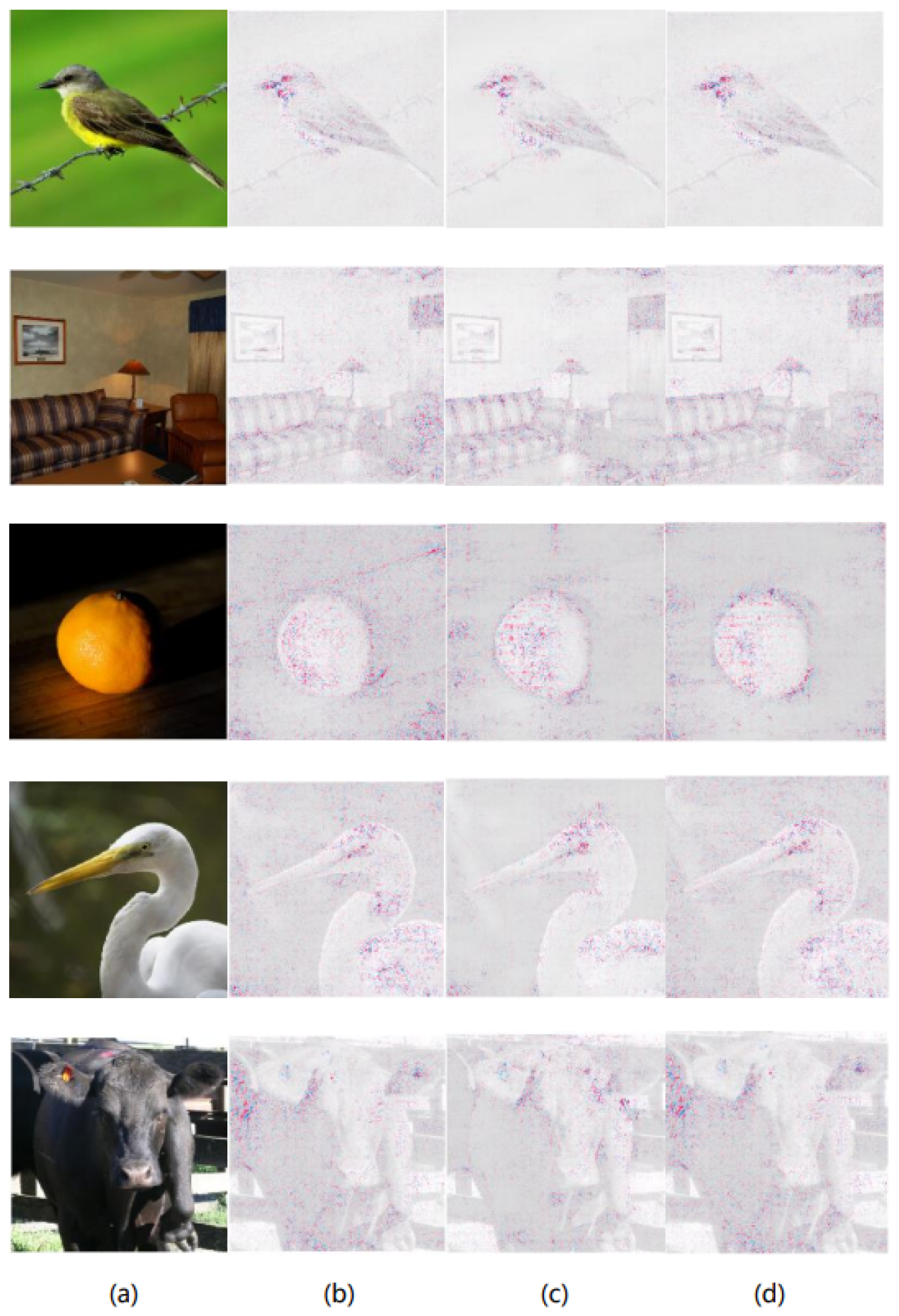
From these visual comparisons, it is evident that for both ResNet50 and VGG16, Expected Gradients (EG) tends to highlight important features distributed in the background rather than on the object itself, which contradicts human intuition. Model-learned features should ideally be object-centric rather than background-related. The proposed deep prior-based baselines—DeepBGMM-EG and DeepMGM-EG—better align with the definition of "missing" and mitigate the attribution of background features to varying extents. These methods concentrate important features more effectively on the object, aligning better with human cognition and providing more faithful explanations of the model’s reasoning. Comparing DeepBGMM-EG and DeepMGM-EG, it is clear that in most cases, DeepBGMM-EG emphasizes object outlines and object-specific features more effectively.
Figure 4.
In the original images of agama and American egret(a), the prediction results of ResNet50 are explained using Expected Gradients (b), DeepBGMM-EG (c) and DeepMGM-EG (d) methods, presenting the corresponding feature attribution maps.
Figure 4.
In the original images of agama and American egret(a), the prediction results of ResNet50 are explained using Expected Gradients (b), DeepBGMM-EG (c) and DeepMGM-EG (d) methods, presenting the corresponding feature attribution maps.
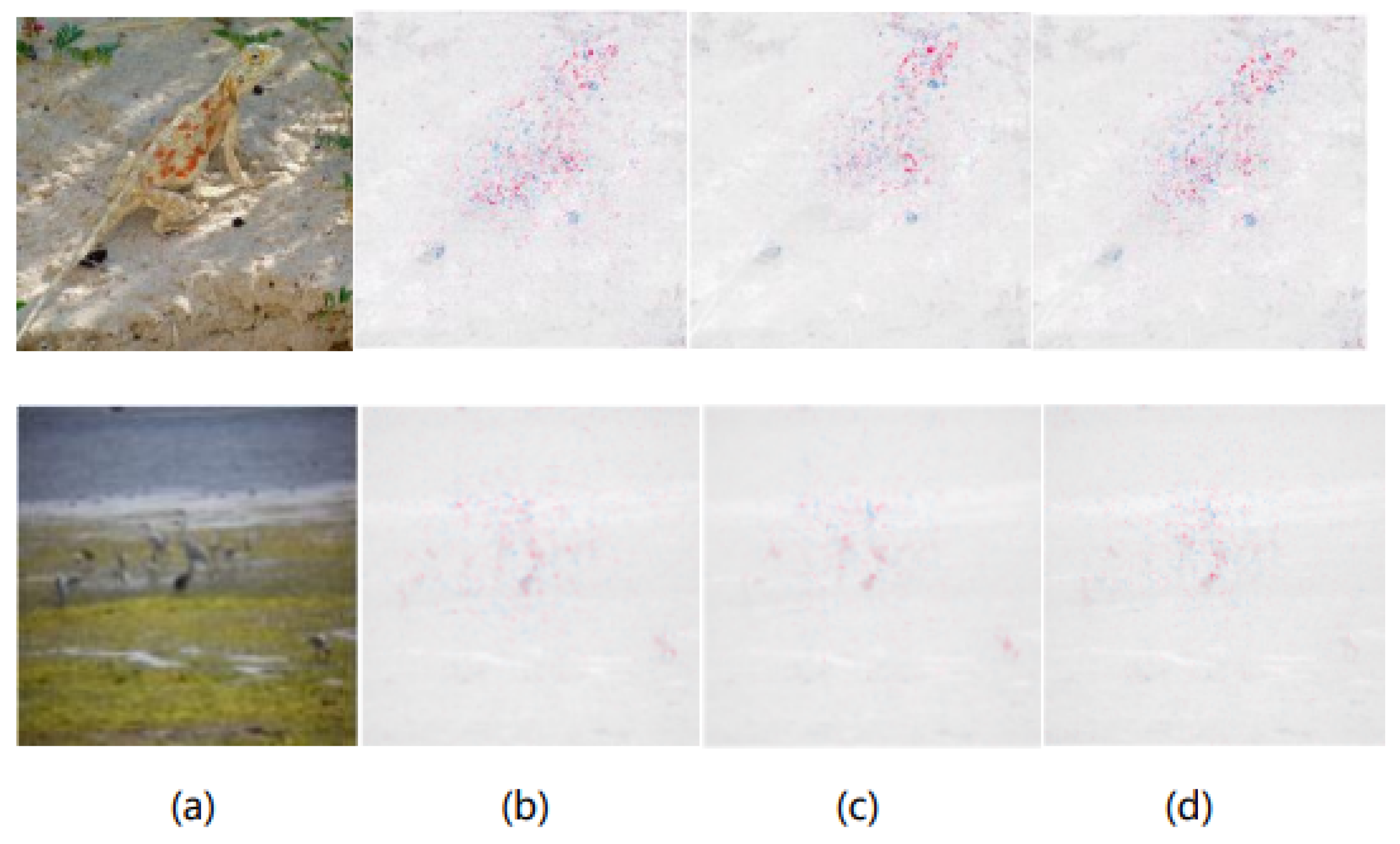
Figure 5.
In the original images of agama and American egret(a), the prediction results of VGG16 are explained using Expected Gradients (b), DeepBGMM-EG (c) and DeepMGM-EG (d) methods, presenting the corresponding feature attribution maps.
Figure 5.
In the original images of agama and American egret(a), the prediction results of VGG16 are explained using Expected Gradients (b), DeepBGMM-EG (c) and DeepMGM-EG (d) methods, presenting the corresponding feature attribution maps.

ResNet50’s attributions proved to be better than those of VGG16 due to the correct prediction of agama, whereas VGG16 incorrectly predicted starfish, which negatively affected the attribution results. From the feature attribution maps generated for the American egret using ResNet50 and VGG16, it is evident that the explanatory results of ResNet50 and the predictive results of VGG16 are suboptimal. This can be largely attributed to the models’ prediction outcomes, as both ResNet50 and VGG16 identified the image as a crane rather than an American egret. Consequently, inaccurate predictions significantly affect the performance of the explanation methods used. We selected 50 images from the ImageNet validation set for each of the 12 categories, resulting in a total of 600 images, to compare the performance of the four explanation methods across the metrics presented in the table.
The performance of EG, DeepBGMM-EG, DeepMGM-EG, and LIFT was compared for ResNet50 in Table 1. DeepBGMM-EG and DeepMGM-EG showed significant advantages in KPM, RNM, and RAM, outperforming other methods in handling feature importance and feature recovery. For KAM, both methods performed similarly to EG, indicating stability in handling important features. In contrast, EG demonstrated stronger performance on KNM and RPM, suggesting greater efficiency in recovering negative feature importance. From the perspective of feature recovery (KPM, KNM, KAM), gradually unmasking features based on their attributed importance (high to low) and observing prediction accuracy can reveal feature importance: significant accuracy improvement indicates higher importance, demonstrating the DeepPrior-EG’s fidelity to the model. Conversely, from the feature masking perspective (RPM, RNM, RAM), gradually masking features (high to low) and observing accuracy can similarly identify important features: significant accuracy decline confirms higher importance, further validating the DeepPrior-EG’s alignment with the model’s behavior. In general, DeepBGMM-EG and DeepMGM-EG outperformed EG in most metrics, particularly in comprehensive assessments of the importance of features.
Similarly, Table 2 reports the comparison for VGG16. DeepBGMM-EG outperformed other methods in KPM, KAM, RPM, RNM, and RAM, demonstrating its strong capability in handling feature importance and recovery, which enhanced model interpretability and reliability. Although EG and LIFT performed comparably on the KNM metric, DeepBGMM-EG exhibited superior performance on most metrics. DeepMGM-EG also performed well but was slightly less effective than DeepBGMM-EG on KPM and KAM. These results indicate that DeepBGMM-EG provides more comprehensive and accurate feature evaluations, contributing to improved interpretability in deep learning models. In general, DeepBGMM-EG performance in VGG16 further validates its potential as an effective interpretability method,In general, DeepBGMM-EG performance in VGG16 further validates its potential as an effective interpretability method, as DeepBGMM-EG demonstrates a stronger alignment with the model’s behavior.
4.3.2. Improving Noise Robustness of Model Re-trained with Attribution Priors
In traditional deep learning training, the optimization objective is to minimize the loss function , where represents the model parameters, X are the input data, and y is the labels. Regularization terms are often added to prevent overfitting, and the optimization problem can be expressed as:
where is the regularization term for the model parameters, and controls the regularization strength.
When incorporating attribution priors, the model must minimize both the loss function and constraints on feature attributions. Let represent the feature attribution matrix, where each element denotes the importance of feature i in sample l. The prior attribution is introduced as a penalty function , with controlling the regularization strength. The optimization objective is modified as follows:
This formulation ensures that the model not only minimizes prediction error but also adheres to attribution constraints, enhancing robustness and interpretability.
In this experiment, we assessed the noise robustness of different models by progressively introducing Gaussian noise into the test data of the MNIST handwritten digit dataset. Four models were evaluated: DeepBGMM-EG (Bayesian prior-based Expected Gradients), DeepMGM-EG (Gaussian prior-based Expected Gradients), EG (standard Expected Gradients), and a baseline model with no attribution priors. The objective was to observe how the classification accuracy of each model changed as the noise level increased.
As shown in Figure 6, the test precision of the four models was plotted against different noise levels, ranging from 0% to 100%. For noise levels below 0.3, all models exhibit similar performance, maintaining a test accuracy close to 0.9, with DeepBGMM-EG and DeepMGM-EG performing slightly better. However, as the noise percentage increased, both DeepBGMM-EG and DeepMGM-EG significantly outperformed the base and EG models, particularly at higher noise levels.
The base and EG models showed a steep decline in accuracy when the noise level exceeded 0.5, indicating poor performance in high-noise environments. In contrast, models trained with prior attribution—especially those using DeepBGMM-EG and DeepMGM-EG—showed notable improvements in noise robustness. These models effectively maintained higher accuracy rates as noise increased from 0.3 to 1.0, highlighting the impact of incorporating prior attribution on improving the model’s resilience to noisy data.
5. Discussion
Based on the experiments conducted in this work, we explored additional dimensions to further validate the effectiveness of the proposed methods. Two supplementary experiments—an evaluation of improved model robustness to noise in a classification task and a comparison using Class Activation Mapping (CAM)—were performed to strengthen our findings.
5.1. Comparison with Shape Priors
We selected 12 categories from the ImageNet 2012 dataset and annotated 50 binary contour images per category, resulting in 600 high-quality shape priors. These annotated images were processed using the PaddleSeg toolkit, which enabled precise annotation and correction of object contours. Figure 7 demonstrates the original and annotated contour images used as shape priors.
To compare the traditional histogram-based shape prior (Shape-EG) with the deep appearance prior based on Bayesian Gaussian Mixture Models (DeepBGMM-EG), it is evident from the metrics that the introduction of the histogram-based shape prior baseline leads to an overall improvement in performance for Shape-EG compared to EG. However, this enhancement is not as significant as that achieved by DeepBGMM-EG, which consistently outperforms Shape-EG across most metrics.
5.2. Comparison of Methods with CAM
To further evaluate the quality of the explanations, we conducted a comparison using Class Activation Mapping (CAM) and calculated Insertion and Deletion scores. These scores are analogous to the Average Drop (AD) and Increase in Confidence (IC) metrics, aiming to assess whether the importance of pixels in CAM maps aligns with the actual relevance of the image content [34]. Specifically, the deletion score measures how much the classification probability drops when important pixels are removed, while the insertion score tracks how much the probability increases when key pixels are added to a blank image. A lower deletion score and a higher insertion score indicate more interpretable and reasonable CAM maps.
The calculation of the Deletion (Del) score follows a specific procedure: pixels corresponding to an image are removed in descending order based on their weights in the Class Activation Map (CAM). The original model is then utilized to compute the classification probabilities for the images after pixel removal. A curve is generated to illustrate the relationship between the classification probabilities and the proportion of removed pixels, and the area under this curve is calculated as the Del value.
Similarly, the process for calculating the Insertion (Ins) score is analogous to that of Del. Pixels are introduced in descending order of their weights, and the original model computes the classification probabilities for the images after pixel addition. A curve is created to represent the relationship between the classification probabilities and the proportion of introduced pixels, with the area under this curve being calculated as the Ins value.
As illustrated in Table 4, the EG-based methods produced the most interpretable and coherent CAM maps, with DeepBGMM-EG achieving particularly strong results. DeepBGMM-EG had the highest Insertion score and one of the lowest Deletion scores, demonstrating its ability to effectively explain the decision-making process of the model. DeepMGM-EG and Shape-EG also performed well, consistently generating reasonable CAM visualizations. However, methods such as Lime and Grad-CAM, while offering some level of interpretability, were outperformed by the EG series in both metrics, highlighting the superiority of the proposed approach.
Summary: The findings from the noise robustness and CAM comparison experiments further confirm the efficacy of the proposed methods. By integrating attribution priors, particularly through DeepBGMM-EG and DeepMGM-EG, the models demonstrate enhanced robustness to noise while producing more interpretable and meaningful feature importance maps. These results underscore the versatility and improved interpretability of these approaches across diverse scenarios, highlighting their potential to advance the robustness, transparency, and reliability of deep learning models in practical applications.
6. Conclusion
In this paper, we introduced a novel framework that enhances the interpretability of deep learning models by incorporating prior-based baselines into the Expected Gradients (EG) method. By leveraging shape and appearance priors, our approach addresses a critical limitation of traditional gradient-based attribution methods: the challenge of selecting appropriate baselines. Our experiments on the ImageNet and MNIST datasets demonstrated that the proposed DeepBGMM-EG and DeepMGM-EG methods significantly outperform existing techniques in focusing on object-specific features while minimizing the influence of irrelevant background information. These improvements were validated across multiple evaluation metrics, underscoring the robustness and effectiveness of our approach. The results highlight the potential of integrating domain-specific priors to align feature attributions more closely with human intuition, thereby providing more accurate and meaningful explanations for model decisions.
Building on the proposed framework, several promising directions for future research emerge. First, exploring alternative methods for computing prior-based baselines—such as task-specific priors or adaptive priors learned directly from data—could further enhance the flexibility and precision of feature attribution. Additionally, investigating advanced feature extraction techniques that combine visual and non-visual priors may yield deeper insights into improving interpretability across diverse applications. Expanding the evaluation to other datasets and models, particularly in high-stakes domains like healthcare, finance, and autonomous systems, would further validate the generalizability and practical impact of our framework. Finally, integrating our prior-based approach with other explainability methods could pave the way for a comprehensive suite of tools to foster trust and transparency in AI systems, ultimately contributing to their broader adoption and responsible use.
Acknowledgments
This work is partly supported by the Special Project of Scientific and Technological Basic Resources Survey of the Ministry of Science and Technology of China under Grant No 2019FY100100, the the Special Project of Natural Science Foundation of China under Grant No 72442029.
Conflicts of Interest
All authors disclosed no relevant relationships.
References
- Wang H, Fu T, Du Y, et al. Scientific discovery in the age of artificial intelligence[J]. Nature, 2023, 620(7972): 47-60. [CrossRef]
- Alowais S A, Alghamdi S S, Alsuhebany N, et al. Revolutionizing healthcare: the role of artificial intelligence in clinical practice[J]. BMC medical education, 2023, 23(1): 689. [CrossRef]
- Khaleel M, Ahmed A A, Alsharif A. Artificial Intelligence in Engineering[J]. Brilliance: Research of Artificial Intelligence, 2023, 3(1): 32-42.
- Nazir S, Dickson D M, Akram M U. Survey of explainable artificial intelligence techniques for biomedical imaging with deep neural networks[J]. Computers in Biology and Medicine, 2023, 156: 106668. [CrossRef]
- Hassija V, Chamola V, Bajpai B C, et al. Security issues in implantable medical devices: Fact or fiction?[J]. Sustainable Cities and Society, 2021, 66: 102552.
- Wichmann F A, Geirhos R. Are deep neural networks adequate behavioral models of human visual perception?[J]. Annual Review of Vision Science, 2023, 9(1): 501-524.
- Hassija V, Chamola V, Mahapatra A, et al. Interpreting black-box models: a review on explainable artificial intelligence[J]. Cognitive Computation, 2024, 16(1): 45-74. [CrossRef]
- Slack D, Hilgard A, Singh S, et al. Reliable post hoc explanations: Modeling uncertainty in explainability[J]. Advances in neural information processing systems, 2021, 34: 9391-9404. [CrossRef]
- Ai Q, Narayanan. R L. Model-agnostic vs. model-intrinsic interpretability for explainable product search[C]//Proceedings of the 30th ACM International Conference on Information & Knowledge Management. 2021: 5-15.
- Song Y Y, Ying L U. Decision tree methods: applications for classification and prediction[J]. Shanghai archives of psychiatry, 2015, 27(2): 130. [CrossRef]
- Su X, Yan X, Tsai C L. Linear regression[J]. Wiley Interdisciplinary Reviews: Computational Statistics, 2012, 4(3): 275-294.
- LaValley M, P. Logistic regression[J]. Circulation, 2008, 117(18): 2395-2399.
- Rigatti S, J. Random forest[J]. Journal of Insurance Medicine, 2017, 47(1): 31-39.
- Kontschieder P, Fiterau M, Criminisi A, et al. Deep neural decision forests[C]//Proceedings of the IEEE international conference on computer vision. 2015: 1467-1475.
- Chen T, Guestrin C. Xgboost: A scalable tree boosting system[C]//Proceedings of the 22nd acm sigkdd international conference on knowledge discovery and data mining. 2016: 785-794.
- Fernando T, Gammulle H, Denman S, et al. Deep learning for medical anomaly detection–a survey[J]. ACM Computing Surveys (CSUR), 2021, 54(7): 1-37. [CrossRef]
- Sundararajan M, Taly A, Yan Q. Gradients of counterfactuals[J]. arxiv preprint arxiv:1611.02639, 2016.
- Shrikumar A, Greenside P, Kundaje A. Learning important features through propagating activation differences[C]//International conference on machine learning. PMlR, 2017: 3145-3153.
- Bach S, Binder A, Montavon G, et al. On pixel-wise explanations for non-linear classifier decisions by layer-wise relevance propagation[J]. PloS one, 2015, 10(7): e0130140. [CrossRef]
- Erion G, Janizek J D, Sturmfels P, et al. Improving performance of deep learning models with axiomatic attribution priors and expected gradients[J]. Nature machine intelligence, 2021, 3(7): 620-631.
- Hamarneh G, Li X. Watershed segmentation using prior shape and appearance knowledge[J]. Image and Vision Computing, 2009, 27(1-2): 59-68.
- Ulyanov D, Vedaldi A, Lempitsky V. Deep image prior[C]//Proceedings of the IEEE conference on computer vision and pattern recognition. 2018: 9446-9454.
- Do C, B. The multivariate Gaussian distribution[J]. Section Notes, Lecture on Machine Learning, CS, 2008, 229.
- Nosrati, Masoud S., and Ghassan Hamarneh. "Incorporating prior knowledge in medical image segmentation: a survey." arXiv preprint (2016). arXiv:1607.01092 (2016).
- Zhao X, Huang W, Huang X, et al. Baylime: Bayesian local interpretable model-agnostic explanations[C]//Uncertainty in artificial intelligence. PMLR, 2021: 887-896.
- Baehrens D, Schroeter T, Harmeling S, et al. How to explain individual classification decisions[J]. The Journal of Machine Learning Research, 2010, 11: 1803-1831.
- Enguehard, J. Sequential Integrated Gradients: a simple but effective method for explaining language models[J]. arxiv preprint arxiv:2305.15853, 2023.
- Sayres R, Taly A, Rahimy E, et al. Using a deep learning algorithm and integrated gradients explanation to assist grading for diabetic retinopathy[J]. Ophthalmology, 2019, 126(4): 552-564.
- Sturmfels P, Lundberg S, Lee S I.Visualizing the Impact of Feature Attribution Baselines[J].Distill, 2020, 5(1). [CrossRef]
- Pignat E, Calinon S. Bayesian Gaussian mixture model for robotic policy imitation[J]. IEEE Robotics and Automation Letters, 2019, 4(4): 4452-4458. [CrossRef]
- Deng J, Dong W, Socher R, et al. Imagenet: A large-scale hierarchical image database[C]//2009 IEEE conference on computer vision and pattern recognition. Ieee, 2009: 248-255.
- Krizhevsky A, Sutskever I, Hinton G E. 2012 AlexNet[J]. Adv. Neural Inf. Process. Syst, 2012: 1-9.
- Lundberg S M, Erion G, Chen H, et al. From local explanations to global understanding with explainable AI for trees[J]. Nature machine intelligence, 2020, 2(1): 56-67. [CrossRef]
- Petsiuk, V. Rise: Randomized Input Sampling for Explanation of black-box models[J]. arxiv preprint arxiv:1806.07421, 2018.
- Lu, J. A survey on Bayesian inference for Gaussian mixture model[J]. arXiv preprint. arXiv:2108.11753, 2021.
Figure 1.
The architecture of DeepPrior-EG.

Figure 2.
In the original images of bulbul, studio couch, orange, American egret and ox (a), the prediction results of ResNet50 are explained using Expected Gradients (b), DeepBGMM-EG (c) and DeepMGM-EG (d) methods, presenting the corresponding feature attribution maps.
Figure 2.
In the original images of bulbul, studio couch, orange, American egret and ox (a), the prediction results of ResNet50 are explained using Expected Gradients (b), DeepBGMM-EG (c) and DeepMGM-EG (d) methods, presenting the corresponding feature attribution maps.
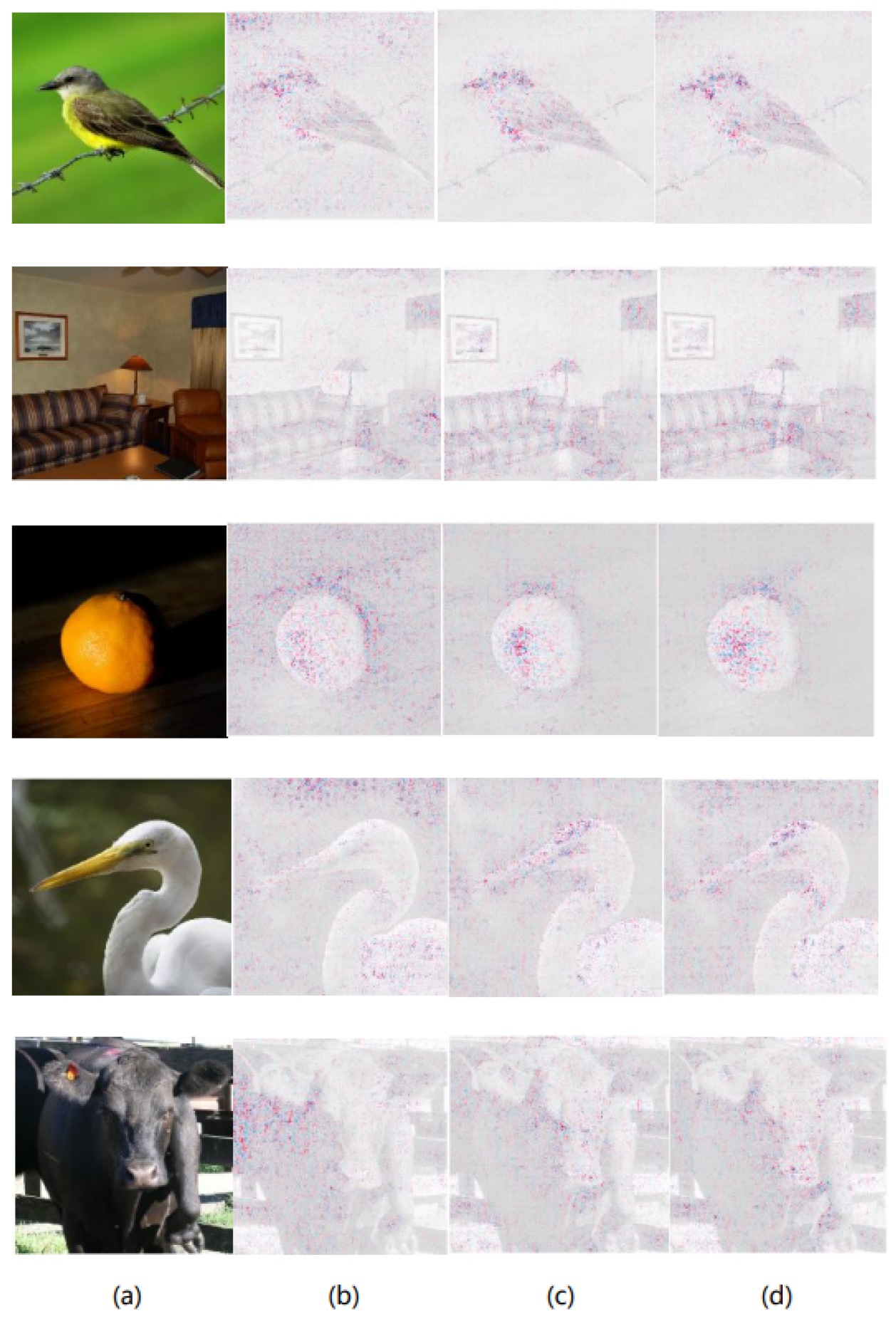
Figure 6.
Accuracy variations in image predictions as Gaussian noise is progressively introduced for four models: Base (without explainability priors, green), EG (blue), DeepBGMM-EG (red), and DeepMGM-EG (yellow). All models were trained with their respective explainability priors except where noted.
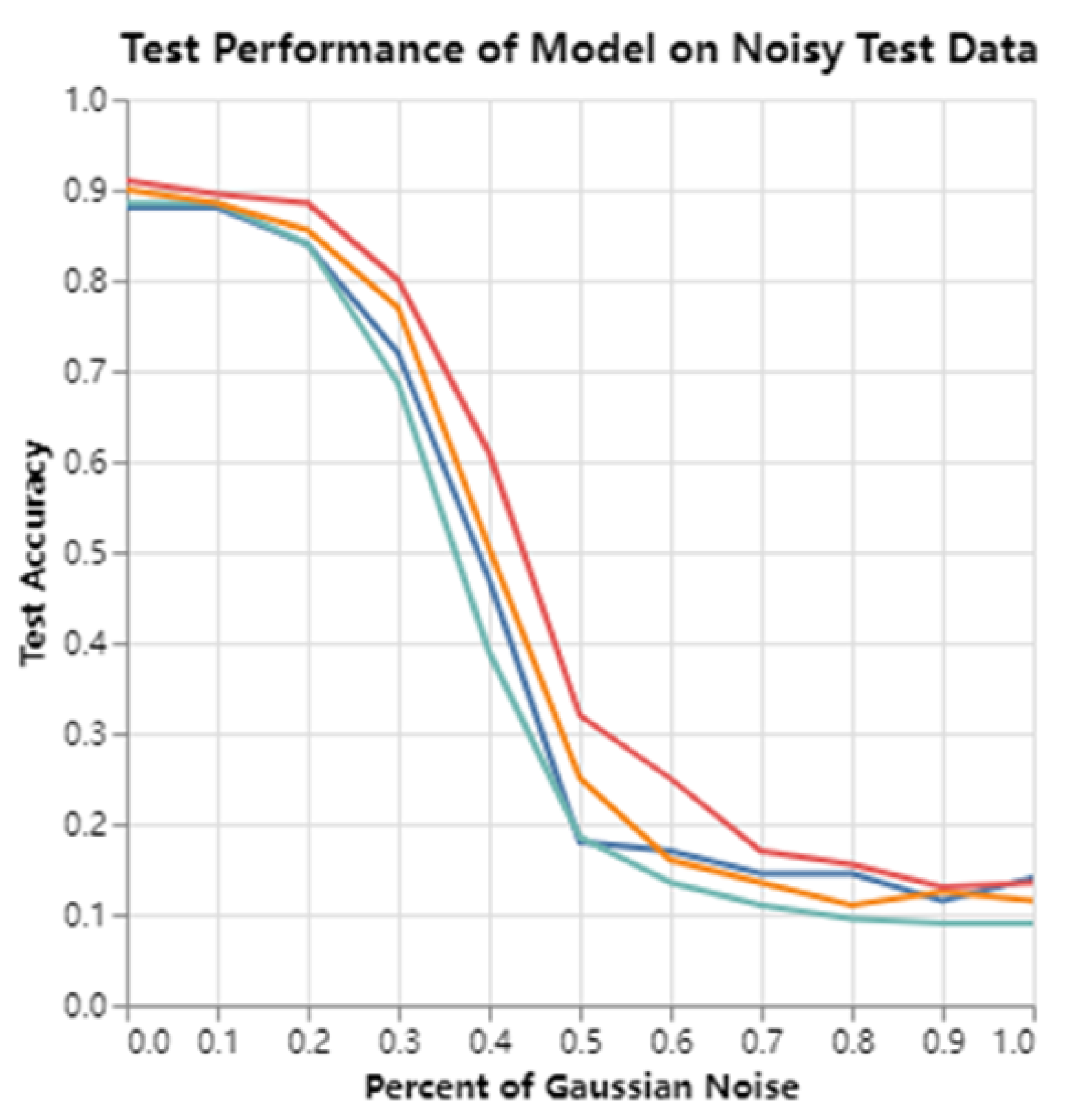
Figure 7.
(a) Original Image (b) Annotated Contour Image.
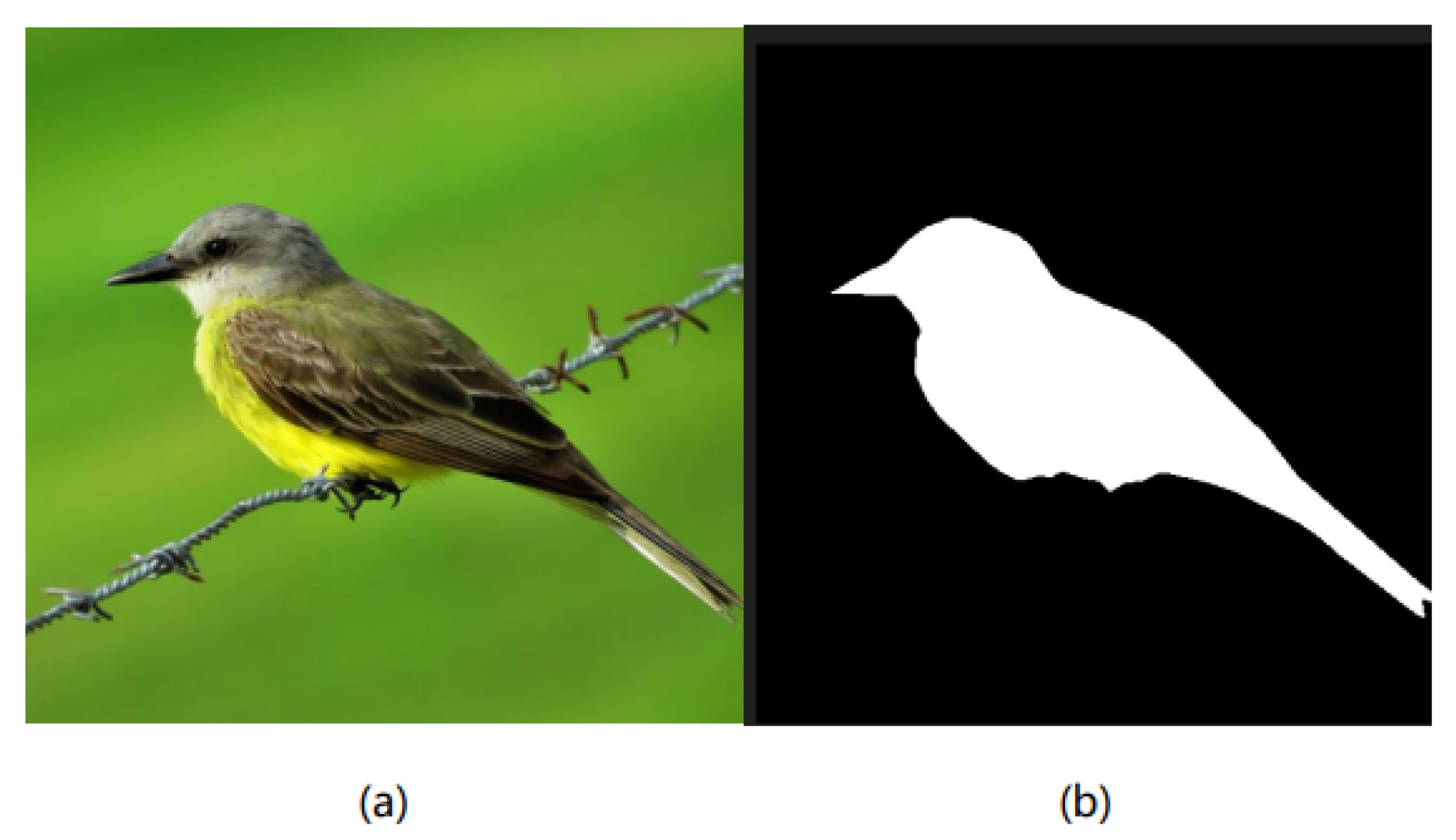

Table 1.
Comparison of different explanation methods (EG, DeepBGMM-EG, DeepMGM-EG, and LIFT) based on various metrics (KPM, KNM, KAM, RPM, RNM, RAM) for ResNet50 predictions. The dataset consists of 600 images selected from the ImageNet validation set, with 50 images per category from 12 categories.
| method | KPM | KNM | KAM | RPM | RNM | RAM |
|---|---|---|---|---|---|---|
| EG | 1.0952 | -1.1014 | 0.9653 | 1.2502 | -1.2558 | 1.4305 |
| LIFT | 1.1027 | -1.1283 | 0.9288 | 1.2120 | -1.2316 | 1.4432 |
| DeepBGMM-EG | 1.1193 | -1.1279 | 0.9580 | 1.2224 | -1.2340 | 1.4361 |
| DeepMGM-EG | 1.1192 | -1.1283 | 0.9565 | 1.2217 | -1.2333 | 1.4342 |
Table 2.
Comparison of different explanation methods (EG, DeepBGMM-EG, DeepMGM-EG, and LIFT) based on various metrics (KPM, KNM, KAM, RPM, RNM, RAM) for VGG16 predictions. The dataset consists of 600 images selected from the ImageNet validation set, with 50 images per category from 12 categories.
Table 2.
Comparison of different explanation methods (EG, DeepBGMM-EG, DeepMGM-EG, and LIFT) based on various metrics (KPM, KNM, KAM, RPM, RNM, RAM) for VGG16 predictions. The dataset consists of 600 images selected from the ImageNet validation set, with 50 images per category from 12 categories.
| method | KPM | KNM | KAM | RPM | RNM | RAM |
|---|---|---|---|---|---|---|
| EG | 1.2418 | -1.2390 | 1.0217 | 2.4655 | -2.4639 | 2.8490 |
| LIFT | 1.0055 | -0.8827 | 0.9758 | 2.7043 | -2.6894 | 2.8403 |
| DeepBGMM-EG | 1.2603 | -1.2412 | 1.0244 | 2.3692 | -2.3510 | 2.7601 |
| DeepMGM-EG | 1.2540 | -1.2416 | 1.0131 | 2.4678 | -2.4566 | 2.8758 |
Table 3.
Comparison of different explanation methods (EG, DeepBGMM-EG,Shape-EG) based on various metrics (KPM, KNM, KAM, RPM, RNM, RAM) for ResNet50 predictions. The dataset consists of 600 images selected from the ImageNet validation set, with 50 images per category from 12 categories.
Table 3.
Comparison of different explanation methods (EG, DeepBGMM-EG,Shape-EG) based on various metrics (KPM, KNM, KAM, RPM, RNM, RAM) for ResNet50 predictions. The dataset consists of 600 images selected from the ImageNet validation set, with 50 images per category from 12 categories.
| method | KPM | KNM | KAM | RPM | RNM | RAM |
|---|---|---|---|---|---|---|
| EG | 1.0952 | -1.1014 | 0.9653 | 1.2502 | -1.2558 | 1.4305 |
| DeepBGMM-EG | 1.1193 | -1.1279 | 0.9580 | 1.2224 | -1.2340 | 1.4361 |
| Shape-EG | 1.1018 | -1.1044 | 0.9649 | 1.2485 | -1.2504 | 1.4317 |
Table 4.
Comparison of Insertion and Deletion Scores for Different Explanation Methods on 600 Images from the ImageNet Validation Set. The table presents the insertion and deletion scores for various explanation methods, showing that the EG-based methods generate more accurate and interpretable CAM visualizations compared to Lime and Grad-CAM.
| method | insertion | deletion |
|---|---|---|
| Lime | 0.1178 | 0.1127 |
| Grad-CAM | 0.1233 | 0.1290 |
| Baylime | 0.1178 | 0.1127 |
| EG | 0.6849 | 0.1206 |
| DeepBGMM-EG | 0.6849 | 0.1202 |
| DeepMGM-EG | 0.6842 | 0.1204 |
| Shape-EG | 0.6841 | 0.1207 |
Disclaimer/Publisher’s Note: The statements, opinions and data contained in all publications are solely those of the individual author(s) and contributor(s) and not of MDPI and/or the editor(s). MDPI and/or the editor(s) disclaim responsibility for any injury to people or property resulting from any ideas, methods, instructions or products referred to in the content. |
© 2025 by the authors. Licensee MDPI, Basel, Switzerland. This article is an open access article distributed under the terms and conditions of the Creative Commons Attribution (CC BY) license (http://creativecommons.org/licenses/by/4.0/).
Copyright: This open access article is published under a Creative Commons CC BY 4.0 license, which permit the free download, distribution, and reuse, provided that the author and preprint are cited in any reuse.


