
Submitted:
29 March 2025
Posted:
01 April 2025
You are already at the latest version
Abstract
Given the variety of focus measure operators, selecting an appropriate one based on scene requirements is critical. Based on the evaluation of the focusing curve morphology and considering the accuracy and robustness of metrics, four metrics were designed: the steep region width (Ws), the steep to gentle ratio (Rsg), the curvature of peak point (Cp), and the relative root mean square error (RRMSE). Several typical focus measure operators were chosen for experimental evaluation. The results demonstrate that the proposed metrics effectively characterize the performance and features of various operators. These metrics serve as a valuable reference for selecting appropriate operators and provide a theoretical foundation for designing new ones.
Keywords:
automatic focusing
; focus measure operator
; Measure indexes
; focusing curve
Highlights
This study proposes a method for determining the cutoff point between steep and gentle regions of focusing curves using multipoint linear fitting, significantly improving adaptability to diverse curve morphologies. Four quantitative metrics namely, Ws, Rsg, Cp and RRMSE were designed to evaluate focus measure operators based on focusing curve morphology were designed to systematically evaluate the sensitivity, robustness, and noise resistance of focus measure operators. These metrics provide a theoretical foundation for optimizing operator selection in autofocus systems and offer insights for designing novel focus algorithms.
What are the main findings?
- Multipoint linear fitting is adopted, and the intersection of fitting lines is used as the cutoff point between the gentle and steep regions of the focusing curve.
- When designing evaluation metrics, considerations were given to the issues of accuracy and robustness of these metrics.
What is the implication of the main finding?
- The method proposed to determine the cutoff point between gentle and steep regions is relatively robust and can adapt to different shapes of focusing curves.
- Provides a theoretical foundation for selecting the optimal focus measure operator and the designing new focus measure operators.
1. Introduction
The focus measure operator, namely focusing function, recognized as a critical tool for assessing image sharpness, has been extensively utilized within the domains of automatic focusing systems and three-dimensional surface reconstruction[1]. Selecting an appropriate focus measure operator based on scene characteristics and system requirements is challenging due to the variety of available operators.
Selecting a focus measure operator requires consideration of multiple factors, such as image content characteristics, real-time performance requirements of the focusing algorithm, and sensitivity to various image quality metrics. The performance of different operators varies significantly under identical scenarios, highlighting the need for objective assessment methods. Frans C.A. Groen and colleagues conducted experimental comparisons of 11 distinct autofocus functions, analyzing them based on metrics such as unimodality, accuracy, repeatability, range, and generality[2]. Similarly, Sun and colleagues compared 18 different focusing algorithms for microscopic images, proposing metrics such as accuracy, range, number of false maxima, width, and noise level to evaluate and rank the performance of operators[3]. Sun and collaborators analyzed the computational speed and operational efficiency of various focus measure operators, utilizing the sharpness of focusing curves as a measure of their sensitivity[4]. Zhai and colleagues conducted an in-depth analysis of focus measure function curves and proposed six quantitative metrics—steep region width, sharpness ratio, steepness, fluctuation in gentle regions, local extremum factor, and sensitivity—to assess operator performance, selecting 12 focus measure operators for comparative measure[5]. Similarly, Said Pertuz and his team explored the application of different focus measure operators in depth recovery, employing these operators in conjunction with depth information to reconstruct three-dimensional topographies, and further evaluated the reconstructed topographies using metrics such as root mean square error in combination with various focus measure operators[6].
Improving existing focus measure operators is also an important research direction[7,8]. This involves using appropriate quantitative metrics to measure the performance of improved operators. Some researchers have designed quantitative metrics from the perspective of focusing on the shape of focusing curve. But the focusing curve will change with the change of the image scene. This may lead to changes in the evaluation index, or even the evaluation index cannot correctly reflect the performance of the operator. Therefore, when designing the evaluation index, the adaptability of the index to the curve shape change should be comprehensively considered to ensure the accuracy and robustness of the index. On the basis of comprehensive consideration of the above issues, this paper designs a quantitative index to measure the performance of focus measure operators.
2. Design of Quantitative Metrics
2.1. Selection of the Cutoff Point
The focusing function value changes rapidly near the focus, resulting in a steep curve, while it changes slowly away from the focus, leading to a relatively flat curve. Therefore, the focusing curve can be segmented into steep region near the focus and gentle region away from the focus, as illustrated in Figure 1.
Determining these cutoff points between the gentle region and the steep region is a critical issue. The focusing curve in the gentle and steep regions has approximately linear sections. These sections can be fitted with straight lines, and the intersection of these lines can be used to determine the horizontal coordinates of the cutoff points. The points on the focusing curve with the same horizontal coordinates as these intersections can then be used as the cutoff points between the gentle and steep regions, as shown in Figure 2. Due to the adoption of multipoint linear fitting, this method of determining the cutoff point has good stability.
The Mean Square Error (MSE) between the focusing curve and the fitted straight line serves as a metric for evaluating the fitting accuracy. For the steep region, the slope is much larger than that of the gentle region, resulting in a significantly larger MSE. This poses challenges when using MSE as a metric in practical applications. In general, as the curve value increases, the slope of the fitted straight line typically increases initially and then decreases. There is a region where the fitted straight line has the maximum slope. This region usually overlaps with the linear region of the steep region. Even if the fitted straight line and the steep region do not completely overlap, the difference in their slopes is minimal. Therefore, the slope of the fitted straight line can serve as a discriminative basis for measuring the fitting accuracy of the steep region. The fitted straight line with the largest slope is considered the fitted straight line of the steep region.
The horizontal coordinates of the intersection points are denoted as klcp and krcp,and the focusing function values are denoted as F(klcp) and F(krcp). Since the focusing curve only takes values at discrete points, and klcp and krcp are not integers, F(klcp) and F(krcp) cannot be directly obtained. The method of linear interpolation is used to obtain the values of F(klcp) and F(krcp).
2.2. Steep Region Width (Ws)
The steep region width (Ws) is an important feature of the focusing curve. A narrow Ws indicates high sensitivity to focus changes, while a wider width suggests lower sensitivity. The Ws is defined in equation (1),

2.3. Steep to Gentle Ratio (Rsg)
The focusing curve is significantly different in steep and gentle region. Generally, the flatter the gentle region is, the steeper the steep region is. In order to comprehensively measure this morphological feature of the focusing curve, the steep to gentle ratio (Rsg) is proposed, which is defined in equation (2),
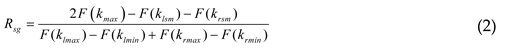
In equation (2), F(kmax) is the peak point of the focusing function. F(klsm) and F(krsm) are the lowest points in the left and right steep regions, respectively. F(klmax) and F(krmax) are the highest points in the left and right gentle regions, while F(klmin) and F(krmin) are the lowest points in those same gentle regions. The Rsg serves as a sensitivity index: a higher value indicates better ability to distinguish between clear and blurred images.
It should be noted that the number of collected Images affects the Rsg index. Therefore, this paper stipulates that the number of collected images should be more than twice the Ws. Generally, as long as this requirement is met, increasing the number of collected images will not significantly change the Rsg index.
2.4. Curvature at Peak (Cp)
For applications such as autofocus systems and shape from focus (SFF), the sensitivity of the focusing function to focus position shift is crucial. The shape of the focusing curve directly reflects the operator’s ability to detect focus position shift. Generally, a steeper focusing curve at its peak indicates greater sensitivity to focus position shift. The peak point of the focusing curve and the focus position generally do not coincide, as shown in Figure 3.
Due to the variability in the distance between the peak point and the focus during each measurement, methods that assess the sensitivity of the focusing function by calculating the distance or slope between the peak point and its neighboring points are not sufficiently robust. Noting that the second-order difference at the peak point changes in the same direction as the absolute value of the first-order difference between two adjacent points, this paper proposes to use the curvature at peak (Cp) to measure the sensitivity of the focus measure operator at the focus, as defined equation (3),
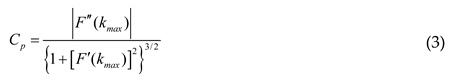
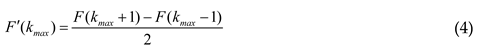
F′(kmax) is the first derivative of the focusing curve at the peak point, as shown in equation (4); F″(kmax) is the second derivative of the focusing curve at the peak point, as shown in equation (5),

The Cp describes the bending degree of the focusing curve at the focus. The greater the Cp, the higher the sensitivity of the operator near the focus is.
2.5. Relative Root Mean Square Error (RRMSE)
During the focusing process, the complexity of the image acquisition environment and image noise can cause the focusing function value to change. To evaluate the performance of different focusing functions under noise, Gaussian white noise was added to the image sequence. After noise processing, the focusing function values generally deviate from the original values, as shown in Figure 4.
A larger deviation between the original curve and the curve added noise indicates reduced robustness of the focusing function. Therefore, this paper proposes using the relative root mean square error (RRMSE) to measure the robustness of the focus measure operator. RRMSE is defined in equation (6).
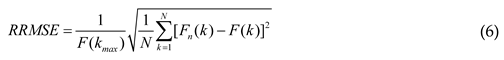
In equation (6), Fn(k) represents the focusing function value after noise processing, and N represents the total number of images. Specifically, a smaller RRMSE indicates stronger resistance to noise interference, suggesting better robustness in practical applications. It should be noted that due to the randomness of noise, the RRMSE may vary with each calculation, but the variation is generally small and negligible.
3. Focus Measure Operators
Focus measure operators based on the spatial domain assess image sharpness by calculating the difference or gradient of a pixel’s gray value. These operators are characterized by low computational effort and good real-time performance [8], making them ideal for real-time applications. In this paper, we select eight spatial-domain focus measure operators that are currently in common use, and use the proposed metrics for quantitative measure.
(1) SMD
The Sum of Modified Differences (SMD) function evaluates the sharpness of an image by summing the absolute values of gray differences between adjacent pixels in the horizontal and vertical directions[9].

(2) Roberts
The squared sum derived from the cross subtraction of the grayscale values of four adjacent pixels is adopted as the gradient value at each pixel in the Roberts operator[10]. The gradient values of all pixels are then summed up to obtain the value of the measure function, as shown in equation (8).

(3) Tenengrad
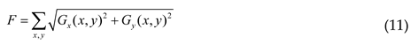
The Tenengrad focus measure function can be viewed as a treatment of Sobel enhancement, which calculates the horizontal and vertical gradients of the image by the Sobel operator, which in turn measures the sharpness of the image edges[11]. Equation (9) and (10) are the horizontal gradient Gx and vertical gradient Gy of the image by the Sobel operator, respectively.
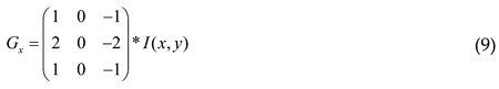
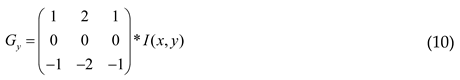
The * in equation (9) and (10) represents the convolution symbol, and the Tenengrad focus measure operator is shown in equation (11).
(4) Brenner
The Brenner focus measure operator is a simple and effective method for image sharpness measurement, which obtains the focus measure value by squaring the difference of adjacent 2-unit image pixel[12].

(5) EOG
Energy of Gradient (EOG) focus measure operator is an image focus measure method based on gradient energy[13]. By calculating the square sum of the difference between the grey values of adjacent pixels in the x and y directions in the image as the evaluation value of each pixel as shown in equation (11).

(6) EOL
The EOL focus measure function is based on the Laplace operator, which is used as the focus measure function by calculating the square of the difference between the center point and the grayscale values in the four directions[14]. As shown in equation (14):

(7) SML
The SML focus measure operator is an improvement upon the EOL operator. It measures image sharpness by calculating the square of the sum of the absolute values of the second-order differences in the horizontal and vertical directions[15]. As shown in equation (15).

(8) Variance
The Variance function is used to measure the degree of dispersion in the distribution of image gray values[16]. And is achieved by calculating the squared cumulative deviation of each pixel’s gray level from the mean value as shown in equation (16).

In equation (16), Ī represents the mean gray value of the image.
4. Experimental Analyses
4.1. Image Acquisition
To validate the performance of different focus measure function metrics, this study constructed a microscopic imaging system, which adopts reflective lighting mode, as shown in Figure 5. The camera used in the setup is the Hikvision MV-CA050-10GM black-and-white camera. The objective lens uses Mitutoyo M Plan APO 10X/0.28. The computer used in the setup runs on the Windows 11(64bit) operating system, equipped with an Intel Corei5-10210U CPU (2.11 GHz) processor.
In the industrial sector, planing and grinding are two common machining processes, and the surface textures produced by these processes show significant differences. The texture of planed surfaces is more complex and irregular. In contrast, the texture of ground surfaces appears as more regular micro-textures in images, with stronger directionality and a gentler overall surface. Utilizing these two types of machined surfaces helps to evaluate the performance of different algorithms when processing various surfaces. In this paper, 90 images were captured from both planed and ground surfaces; some examples are shown in Figure 6.
4.2. Analysis of Results
In order to facilitate the comparison of the performance of different focusing functions, it is generally necessary to normalize the function values. This study employs individual function normalization, which each focusing function is divided by its maximum value.
The normalized focusing curves derived from the planed surface images using different focus measure operators are illustrated in Figure 7.
The normalized focusing curves derived from the ground surface images using different focus measure operators are illustrated in Figure 8.
The metrics proposed in Section 2 are used to analyze different focus measure operators. The fitted straight line consists of 7 points. In order to verify the RRMSE index, Gaussian white noise with variance of 5 is added to the images.
The metrics from the planed surface images are shown in Table 1.
The metrics from the ground surface images are shown in Table 2.
Based on their metrics, the focus measure operators can be divided into two main groups: SMD, Roberts, Tenengrad, and Variance in one category, and Brenner, EOG, EOL, and SML in the other. The former show wider Ws and smaller Rsg and Cp, while the latter show narrower Ws and larger Rsg and Cp. The former reduces the nonlinear amplification effect brought by the squaring operation, making it less sensitive but more robust. The latter amplifies the effect of gradient changes by squaring operation, thus highlighting the edges and details of the image more. These operators are more sensitive to changes in the sharpness of the image, with higher sensitivity.
A side-by-side comparison of the three operators (SMD, Roberts, and Tenengrad) reveals that there is little difference in Cp and Ws. The Rsg metric of SMD operator is large, and the RRMSE metric of Tenengrad operator is small. The Variance operator exhibits the largest Ws metric among all operators, the best RRMSE metric, and the worst Rsg and Rpg metrics.
The four operators Brenner, EOG, EOL and SML can be categorized into two groups. Brenner belongs to one group with EOG. EOL and SML belong to one group. The former has better robustness, while the latter has higher sensitivity.
The sensitivity indices of the Brenner and the EOG operators shows no significant difference. The EOG holds a slight advantage in Rsg. In contrast, in the RRMSE index, the Brenner operator demonstrates a greater advantage.
The SML operator is an improved form based on the EOL operator, which avoids the problem of positive and negative difference cancelation by calculating the gradient change in the horizontal and vertical directions separately, and adding the absolute value operation to the second-order difference in each direction. It can be seen that the difference between the EOL operator and the SML operator is very small in terms of the sensitivity index, but the SML operator is better than the EOL operator in terms of the RRMSE index, which indicates that the SML operator has a better robustness. In general, both of them have outstanding sensitivity but poor robustness.
In summary, the EOL and SML operators exhibit the highest sensitivity but demonstrate limited robustness. The performance of the Variance operator is more extreme, showing the best robustness but poor sensitivity. The Brenner and Tenengrad operators strike a relatively good balance between sensitivity and robustness.
From the experimental results, it can be seen that, although the application scenarios are different, the results of the proposed metrics are basically consistent on both the planed and ground surfaces. Combined with the analysis of the algorithmic principles of various focus measure operators, the proposed metrics are reasonable and can effectively distinguish the differences between different focus measure operators. Researchers can weigh the sensitivity, robustness, and computational complexity of operators based on scene requirements, enabling optimal selection of focus measure operators using the proposed metrics. Meanwhile, these metrics also provide a theoretical foundation for designing new ones.
5. Conclusions
This study quantitatively assesses the performance of focus measure operators by analyzing the shape of the focusing curve. The focusing curve can be divided into steep and gentle regions, with the division method being a critical aspect. A method to divide the steep and gentle regions was proposed. Four metrics, namely, Ws, Rsg, Cp, and RRMSE were designed. To validate their effectiveness, commonly used operators were selected for experimental testing. The results show that the proposed metrics are basically consistent in different scenarios. They can effectively evaluate the performance of different operators. These metrics provide a theoretical foundation for the selection of appropriate operators in tasks such as autofocus systems.
Acknowledgments
This work was supported by Natural Science Foundation of Heilongjiang Province of China (LH2022F028).
Conflicts of Interest
The authors declare that they have no known competing financial interests or personal relationships that could have appeared to influence the work reported in this manuscript.
References
- Nayar, S.K.; Nakagawa, Y.J.I.T.o.P.a.; intelligence, m. Shape from focus. 1994, 16, 824–831.
- Groen, F.C.; Young, I.T.; Ligthart, G. A comparison of different focus functions for use in autofocus algorithms. Cytometry 1985, 6, 81–91. [Google Scholar] [CrossRef] [PubMed]
- Sun, Y.; Duthaler, S.; Nelson, B.J. Ieee. Autofocusing algorithm selection in computer microscopy. In Proceedings of the IEEE/RSJ International Conference on Intelligent Robots and Systems, Edmonton, CANADA, 2005 Aug 02-06, 2005; pp. 419–425.
- Sun, J.; Yuan, Y.; Wang, C. Comparison and Analysis of Algorithms for Digital Image Processing in Autofocusing Criterion %J Acta optica sinica. 2007, 35-39.
- Zhai, Y.; Zhou, D.; Liu, Y.; Liu, S.; Peng, K. Design of Evaluation Index for Auto-Focusing Function and Optimal Function Selection %J Acta optica sinica. 2011, 31, 242–252.
- Pertuz, S.; Puig, D.; Angel Garcia, M. Analysis of focus measure operators for shape-from-focus. Pattern Recognition 2013, 46, 1415–1432. [Google Scholar] [CrossRef]
- Zhang, L.; Tian, Y.; Yin, Y. An Improved Image Sharpness Assessment Method Based on Contrast Sensitivity. In Proceedings of the Conference on Applied Optics and Photonics (AOPC) - Image Processing and Analysis, Beijing, PEOPLES R CHINA, 2015 May 05-07, 2015.
- He, C.; Li, X.; Hu, Y.; Ye, Z.; Kang, H. Microscope images automatic focus algorithm based on eight-neighborhood operator and least square planar fitting. Optik 2020, 206. [Google Scholar] [CrossRef]
- Zhang, J.; Zhang, T. Focusing Algorithm of Automatic Control Microscope Based on Digital Image Processing. Journal of Sensors 2021, 2021. [Google Scholar] [CrossRef]
- Sha, X.; Wang, P.; Shan, P.; Li, H.; Li, Z. A fast autofocus sharpness function of microvision system based on the Robert function and Gauss fitting. Microscopy Research and Technique 2017, 80, 1096–1102. [Google Scholar] [CrossRef] [PubMed]
- Ko, P.; Li, D.; Hoenig, P.; Bailey, I.; Rempel, D. Effect of computer monitor distance on visual symptoms and changes in accommodation and binocular vision. In Proceedings of the Proceedings of the Human Factors and Ergonomics Society Annual Meeting, 2009; pp. 1447–1451.
- Brenner, J.F.; Dew, B.S.; Horton, J.B.; King, T.; Neurath, P.W.; Selles, W.D. An automated microscope for cytologic research a preliminary evaluation. The journal of histochemistry and cytochemistry : official journal of the Histochemistry Society 1976, 24, 100–111. [Google Scholar] [CrossRef] [PubMed]
- Li, Z.; Dong, J.; Zhong, W.; Wang, G.; Liu, X.; Liu, Q.; Song, X. Motionless shape-from-focus depth measurement via high-speed axial optical scanning. Optics Communications 2023, 546. [Google Scholar] [CrossRef]
- Russell, M.J.; Douglas, T.S. Ieee. Evaluation of autofocus algorithms for tuberculosis microscopy. In Proceedings of the 29th Annual International Conference of the IEEE-Engineering-in-Medicine-and-Biology-Society, Lyon, FRANCE, 2007 Aug 22-26, 2007; pp. 3489–+.
- Fu, B.; He, R.; Yuan, Y.; Jia, W.; Yang, S.; Liu, F. Shape from focus using gradient of focus measure curve. Optics and Lasers in Engineering 2023, 160. [Google Scholar] [CrossRef]
- Wang, Y.; Jia, H.; Jia, P.; Chen, K.; Zhang, X. A novel algorithm for three-dimensional shape reconstruction for microscopic objects based on shape from focus. Optics and Laser Technology 2024, 168. [Google Scholar] [CrossRef]
Figure 1.
Diagram of the focusing curve.
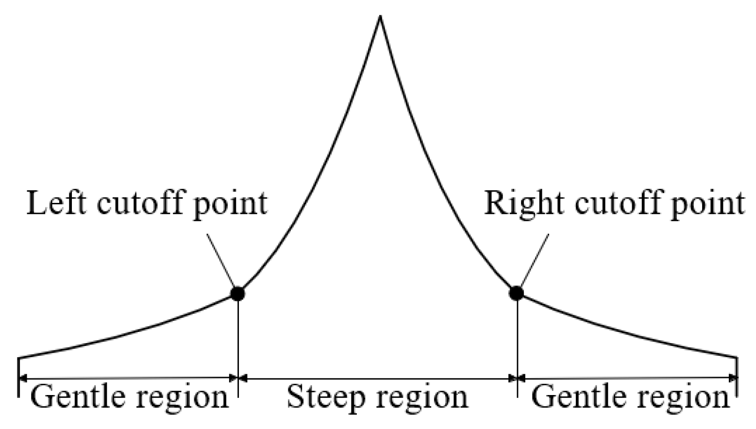
Figure 2.
Diagram of the left and right cutoff points.
Figure 3.
Peak point out of focus.
Figure 4.
Comparison of curve added noise and original curve.
Figure 5.
Microscopic imaging system.
Figure 6.
Planed surface image:(a)1st, (b)45th, (c)90th; Ground surface image: (d)1st, (e)45th, (f)90th.
Figure 6.
Planed surface image:(a)1st, (b)45th, (c)90th; Ground surface image: (d)1st, (e)45th, (f)90th.
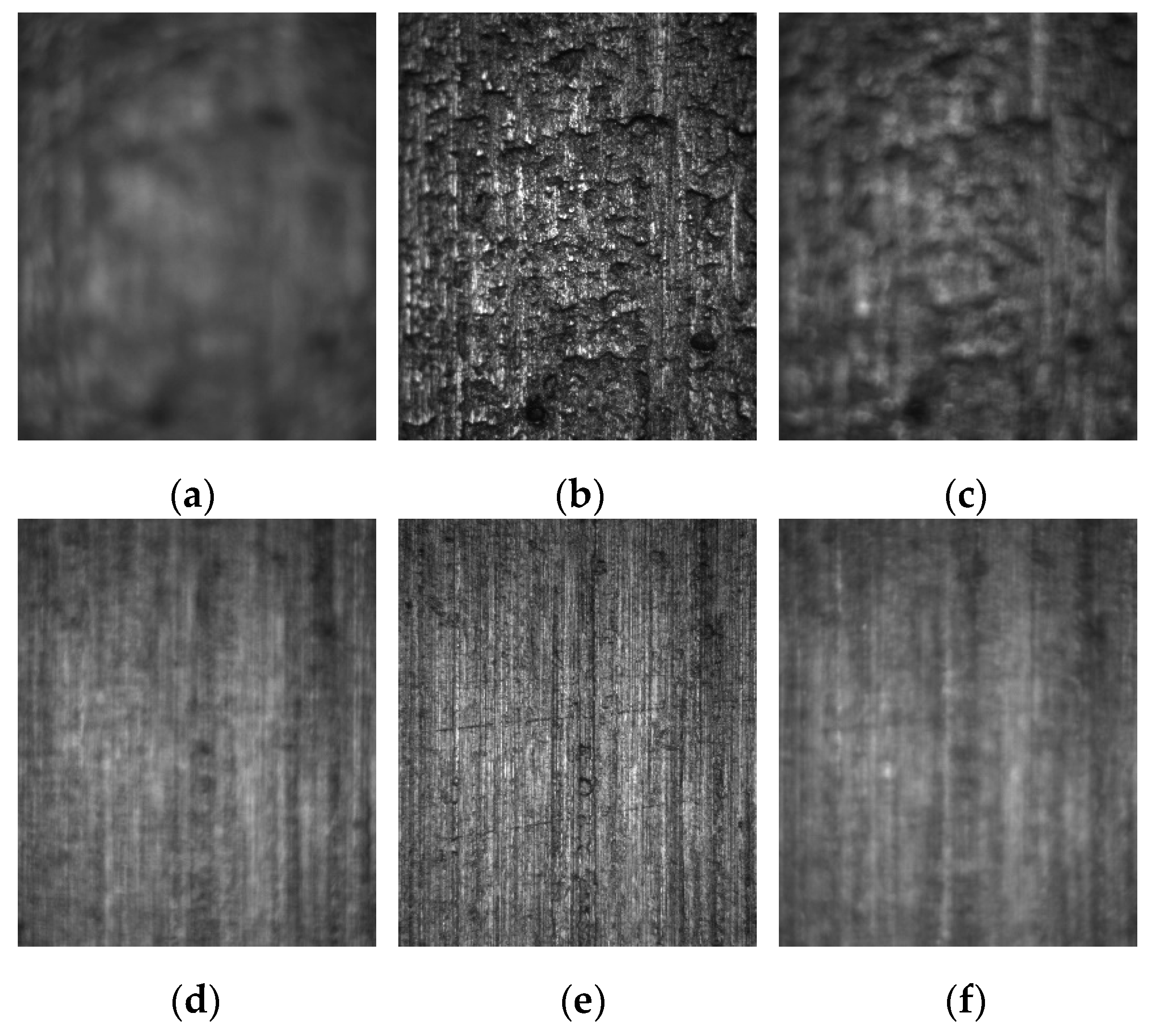
Figure 7.
Focusing curves from the planed surface images.
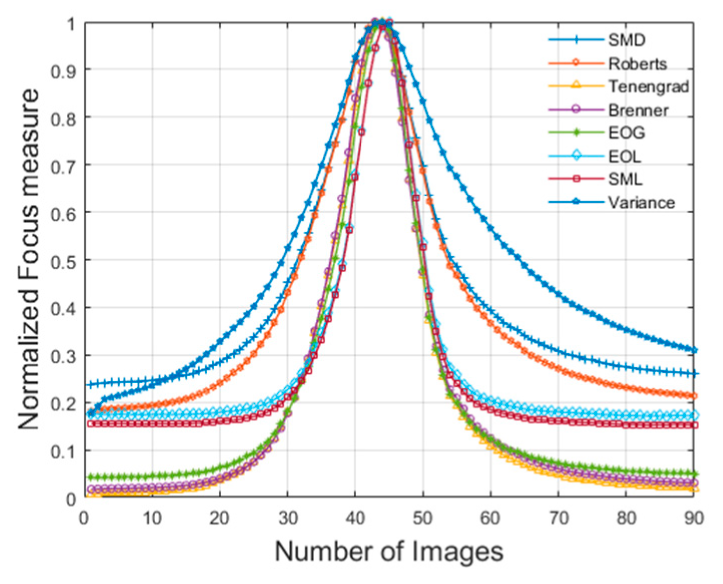
Figure 8.
Focusing curves from the ground surface images.
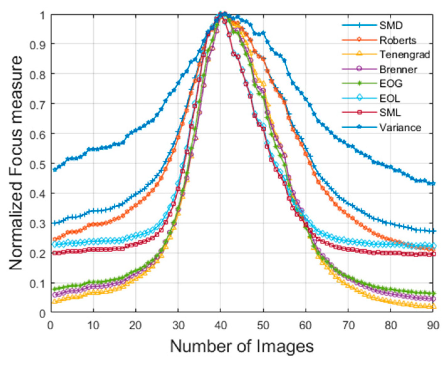

Table 1.
Metrics comparison of different operators (Planed Surface).
| SMD | Roberts | Tenengrad | Brenner | EOG | EOL | SML | Variance | |
|---|---|---|---|---|---|---|---|---|
| Ws | 30.18 | 31.82 | 32.19 | 24.44 | 23.92 | 21.21 | 21.34 | 35.83 |
| Rsg | 3.8391 | 3.4109 | 3.0901 | 4.6899 | 5.1242 | 6.6608 | 6.7004 | 2.2664 |
| Cp | 0.0159 | 0.0156 | 0.0153 | 0.0085 | 0.0307 | 0.0303 | 0.0489 | 0.0500 |
| RRMSE | 0.1679 | 0.0756 | 0.0400 | 0.0375 | 0.0949 | 0.4133 | 0.3687 | 0.0041 |
Table 2.
Metrics comparison of different operators (Ground Surface).
| SMD | Roberts | Tenengrad | Brenner | EOG | EOL | SML | Variance | |
|---|---|---|---|---|---|---|---|---|
| Ws | 40.00 | 40.90 | 41.20 | 36.75 | 36.00 | 31.53 | 31.75 | 41.73 |
| Rsg | 3.4043 | 2.8756 | 2.6686 | 4.7012 | 5.3235 | 6.3045 | 6.2466 | 2.2776 |
| Cp | 0.0123 | 0.0122 | 0.0121 | 0.0091 | 0.0250 | 0.0241 | 0.0381 | 0.0395 |
| RRMSE | 0.1278 | 0.0521 | 0.0247 | 0.0594 | 0.0991 | 0.3998 | 0.3505 | 0.0050 |
Disclaimer/Publisher’s Note: The statements, opinions and data contained in all publications are solely those of the individual author(s) and contributor(s) and not of MDPI and/or the editor(s). MDPI and/or the editor(s) disclaim responsibility for any injury to people or property resulting from any ideas, methods, instructions or products referred to in the content. |
© 2025 by the authors. Licensee MDPI, Basel, Switzerland. This article is an open access article distributed under the terms and conditions of the Creative Commons Attribution (CC BY) license (http://creativecommons.org/licenses/by/4.0/).
Copyright: This open access article is published under a Creative Commons CC BY 4.0 license, which permit the free download, distribution, and reuse, provided that the author and preprint are cited in any reuse.


