
Submitted:
01 April 2025
Posted:
01 April 2025
You are already at the latest version
Abstract
With random graph generation, most of the previously described algorithms were not related to graphs arising in any particular subject area, so in this paper we generate random graphs for a specific area, namely, models of real communication networks. In the paper we propose a method that determines the “best” invariant; the corresponding basic algorithm is as follows. For the generated set of graphs, we calculate the numerical values of each of the pre-selected invariants. For all graphs, we arrange these numerical values in descending order, after which, for each of the 10 pairs of invariants, we calculate the rank correlation of these orders; for such calculations, we use 5 different variants of rank correlation algorithms. In such a way, we get 10 pairs of rank correlation values, then we arrange them as the values of 10 independent elements of the 5x5 table (rows and columns of this table correspond to the 5 invariants under consideration). If the rank correlation values are negative, we record the absolute value of this value in the table. The basic idea is that the “most independent” invariant of the graph gets the minimum sum when summing 4 values of its row, i.e. less than for other invariants (other rows). For our subject area, we got the same result for 5 different variants of calculating the rank correlation: the value obtained for the vector of second-order degrees is significantly better than all the others, and among the usual invariants, the global clustering coefficients invariant is significantly better than others ones; this fact corresponds to our previous calculations, in which we ordered the graph invariants according to completely different algorithms.
Keywords:
random graph
; communication networks
; rank correlation
; Graovac-Ghorbani index
; graph invariants
; global clustering coefficient
MSC: 05C09; 05C07; 05C99; 05C85; 60E99
1. Introduction
At the beginning, We should note that an alternative, and longer and more complete, title of the paper could be as follows: “Random graphs, generated according to the Erdős – Rényi algorithm, as models of communication networks, some of their invariants and a statistical study of the values of these invariants using various rank correlation algorithms”. This title can be even considered as a very brief summary of the entire paper.
Then let us move on to a brief description of modeling large communication networks. Modeling of such high-dimensional networks usually involves not only the generation of graphs of communication networks, but also the so-called flow matrix. Such matrix is a set of pairs of vertices with certain characteristics assigned to each pair. Based on the flow matrix, communication channels are organized, and communication nodes are equipped with equipment and other technical and organizational resources are allocated.
An interesting subject of research is precisely the generation of the flow matrix. This process can be identified with the generation of so-called social connections in random graphs. That is, the edges of random graphs can be considered as a kind of flow in the communication network between some communication nodes.
As practice shows, there are various “drawings” of the flow matrix. In particular, the fact of the occurrence of triangles may be typical for one user of communication services and less typical for another user. The patterns of the appearance of such triangles and some other “unsuccessful” constructions during random graph generation are described in [1,2] etc.; we also note the mention of such constructions in a paper [3] related to another field, namely AI. Therefore, it is necessary to consider various models for generating scale-free graphs, namely edges in them to approximate the behavior of a particular user of the communication network. In addition, when generating, attention should be paid to the connectivity of so-called supergraph forming the flow matrix, since this fact is an indicator of the reliability of the model of random generation of the flow matrix.
In general, the generation of random graphs is extremely relevant due to the need for a test base for an extremely popular task in communication networks, called the organization of a digital transmission system. In order to increase the efficiency of software development that solves such problems, it is advisable to pay attention to the qualitative modeling of the flow matrix in communication networks. This, in turn, will be a qualitative step towards the development of a digital twin of the communication network.
At the same time, such a question may arise. In some previous publications ([5,6], see also some little discussion in the next sections), we considered “in what order” several invariants from a given set (of invariants) should be considered: in order to “more quickly” obtain a result on the non-isomorphism of any two given graphs of the set under consideration (i.e., in our case, graphs of different communication network models); then why conduct further research if we can relatively quickly determine such an order? The answer to this question is the following: we set a more general task by examining the same invariants. Exactly, we set the following problem: does a certain graph belong to some set of graphs? (We repeat that in the case considered in the paper, we mean communication network models.) Of course, this question can only be answered with some degree of certainty.
At the end of the introduction, we note that, of course, we are familiar with the monograph [4] and other publications on similar topics; however, they seem to be of interest only from a theoretical point of view and are unlikely to have an impact on the practical creation of algorithms related to the study of various invariants of specific random graphs.
Here is a summary of the paper by sections.
In Section 2 (“Motivation”), we formulate an approach to a possible solution to the problems of classification and clustering of a certain set of graphs, in particular, to the models of real communication networks.
A brief outline of algorithms considered in this paper is discussed in Section 3.
In Section 4, we consider the description of the special graph invariant, i.e., the second-order degree vector. And the main material of Section 5 (“Description of the second-order degree vector as a numerical invariant of the graph”) is not only the continuation of such description, but also the formulation of an algorithm that reduces this invariant to a numerical characteristic; all this is done in the form of an injective function.
Section 6 (“On the used standard statistical characteristics”) it can be considered as some part of preliminaries. The content of this section is clear from its title. In addition to the standard algorithms for calculating rank correlation described in it, we shall consider the original algorithms in Section 7 (“The proposed approach to calculation of the pair correlation”).
A brief description of the results of computational experiments is given in Section 8.
Section 9 is the conclusion, In it, we briefly define the directions of further work related to the topics discussed in the paper.
We also note that the data sets according to which the calculations were performed in this paper, in particular the generated graphs, are available in the archive, which can be downloaded from the link https://disk.yandex.ru/d/Ad3EiIAMZDRQeg. In the text of the paper, we shall explain the formats of the data provided there, as necessary.
2. Motivation
Obviously, graph invariants can be used to check the non-isomorphism of two graphs. When developing heuristic algorithms that perform such verification, the question often arises about which invariants and in which order it is desirable to check in order to get an answer to this question faster. At the same time, as a rule, the term “faster” requires a special mathematical justification, related, in particular, to the specific algorithms used for generating (obtaining) processed graphs. However, we shall not raise this issue in this paper, we shall only provide the link [6], some related papers in Russian were also published.
However, in this paper we shall try to apply algorithms for calculating graph invariants to other problems. All the invariants known to the authors are set in such a way that for similar graphs (for example, those differing only in the presence/absence of one or two edges), the invariants have similar values. In this way, in the future we shall be able to formulate an approach to a possible solution to the problems of classification and clustering of a certain set of graphs under consideration, in particular, to the models of real communication networks.
In this section, we look at simpler examples, which, apparently, cannot yet be called models of communication networks. We randomly generate several graphs according to the Erdős – Rényi algorithm (9 pieces), and these graphs are obtained for a different number of vertices (10, 20, or 30) and for different saturation (i.e., different probabilities of each edge, namely , , and ). After that, for each of these 9 graphs, we also consider randomly generated changes to it; exactly, for each of the originally generated graphs, we add either 1 random edge (5 variants for each original graph) or 2 random edges (3 variants each). Using the described actions, we get 81 source graphs, while, as follows from the previous one, we specially generated them so that they are clearly divided into 9 clusters of 9 graphs in each cluster. All these randomly generated graphs are listed in the “simple” folder of the aforementioned archive, the format of each graph is obvious.
Next, we consider several invariants for all 81 graphs. In order to actually confirm the assumption that “similar graphs have similar invariants”, there are two of the following ways to proceed.
- (1)
-
For each of the 9 generated graphs, calculate the average values:
- (a)
- for all those generated from it,
- (b)
- for all the others ones;
and the same is for each invariant; we have to get the difference. - (2)
- For some ordering of the graphs (for instance, the one that exists according to the numbers we use), calculate the rank correlation lists of invariants; in this case, sufficiently large values of the correlation coefficients should be obtained.
Here are brief calculation results, most of which can be seen in the file “OUTPUT.xlsx” of the mentioned archive.
- (1)
- Everything turns out quite well, the hypothesis is confirmed.
- (2)
- The GCC invariant stands apart from the other three and correlates little with them; the remaining 3 are interconnected (3 pairs of lists of values, for each pair there are 4 ways to calculate the correlation, for a total of 12 values). We obtained these 12 values in the range from to (the average value is , although it is unlikely that this average value has any meaning), which also confirms the hypothesis.
3. The General Description of the Work Performed
Now let us move on to the description of the main ideas and provisions of this paper. All further randomly generated graphs, as well as the calculation results, are listed in the “main” folder of the aforementioned archive.
As we said before, earlier, in previous publications [5,6,7,8] (see also [9]), we investigated graph invariants, in particular, we determined in which order it is desirable to check them in order to positively answer the question about this in the shortest average time in case of their non-isomorphism; usually, a set of invariants was set in advance. It is important to note that
the work described in the paper can be generalized: not only for some other subject area and corresponding generating algorithms, but also for some other set of invariants.
In the paper, we propose a method that determines “the best” invariant for the subject area under consideration. Thus, with continued research and computational experiments, we shall obtain a sequence of invariants in descending order of preference for their verification; it is clear that this sequence should depend on the considered subject area. We hope that this sequence of invariants will be similar to the sequence we built earlier using completely different algorithms (“similar” means that the coefficient of rank correlation between the sequences will significantly exceed ); at least, preliminary computational experiments confirm this hypothesis. It is worth noting that the main application of rank correlation for this paper will be discussed some later.
Now it is necessary to say which graph invariants we are considering in this paper. These are the following ones:
Next, we shall use exactly this order of these invariants 2.
The basic algorithm that we use for our method is as follows. For a selected set of graphs (in our case, for 81 graphs of “medium” size generated using the Erdős – Rényi model), we calculate the numerical values of each of the 5 selected invariants; remark that for an invariant representing a vector of second-order degrees that does not have an explicit numerical value, we describe a possible variant of the injective mapping that gives such a value (Section 5).
Then we arrange these numerical values in descending order, after which, for each of the 10 pairs of different invariants, we calculate the rank correlation of these orders; note that for such calculations, we use 5 different variants of rank correlation algorithms. Thus, we get 10 pairs of rank correlation values, we arrange them as the values of 10 independent elements of the table (rows and columns of this table correspond to the 5 invariants under consideration); so, for each variant of calculating the rank correlation (recall that this number for our article is also 5), we get a similar table. With negative values of the rank correlation (this rarely happened in our calculations, in less than of cases), we record the absolute value of this value in the table.
Our basic idea is that the “most independent” invariant of the graph gets the minimum sum when summing 4 values of its row, i.e. less than for other invariants (other rows). For our subject area, for any of the 10 counting options 3, the result is the same: the value obtained for the vector of second-order degrees is significantly better than all the others. Among the “usual” invariants (i.e., without considering the vector of second-order degrees), the global clustering coefficients invariant is significantly better than others ones. Again, this roughly corresponds to our previous calculations, in which we ordered the graph invariants according to completely different algorithms 4
4. The Second-Order Degree Vector
Apparently, the least well-known among the listed invariants is the vector of second-order degrees, so let us talk about it in more detail. However, the proposed article is not on pure mathematics, but on mathematical modeling and heuristic algorithms, so in this section we will limit ourselves to an example; this example, we hope, will completely clarify everything. A strict definition of the algorithm will be given below.
Thus, on Figure 1 we see an example of the graph with the designation of the number of vertices adjacent to each one. Therefore, the vector of degrees (of the first order) is obtained as follows:
(in the literature, square brackets are more often used instead of round ones), The vector of degrees of the second order is as follows:
here, the order of the vertices of external level is as follows:
Certainly, both of these options are graph invariants.
At the same time, we note that we write out the usual vector of degrees in the order of non-growth of elements, and the elements of the vector of degrees of the second order are also naturally ordered, which is easy to see based on the example considered 5.
However, it is not difficult to notice the following. Of course, based on the above description, it is simply to formulate a strict definition of this invariant. But such a strict definition does not agree with the work plan of the paper briefly described above, exactly that numerical values of graph invariants are needed to calculate any variants of the correlation coefficient. A similar reduction of the described invariant to a number, while designed as an injective mapping, will be considered in the next section.
5. The Second-Order Degree Vector as a Numerical Invariant
The full name of this section could be as follows: “Description of the second-order degree vector as a numerical invariant of the graph”.
Thus, let us describe the strict definition of the second-order degree vector and its reduction to the number; at the same time, it must have the above-mentioned convenient properties. We repeat once again, that for the material in this section, stricter definitions and constructions are needed than for the previous one.
Let be an undirected graph, where V is the set of vertices and E is the set of edges. For it:
- let be the number of vertices;
- the degree of vertex v denoted is the number of edges incident to v;
- the set of neighbors of vertex v is denoted by ;
- sorted neighbor degrees: for each vertex v, let be the list of degrees of its neighbors sorted in descending order, where and .
Next, the algorithm for constructing the vector of second-order degrees (i.e., the main object of this section) is described. Since the algorithm is constructive, it can be considered as the definition of such a vector.
Step 1: Ordering vertices with comparison function .
We define a comparison function to order the vertices. This function returns:
- a positive value, if v is considered greater than w;
- a negative value, if v is considered less than w;
- 0, if v and w are considered equal.
Denoting and , the comparison function is defined as follows.
-
Compare and :
- if , then v is greater than w;
- if , then v is less than w;
- if , proceed to the next step.
-
For to p (assuming ):
- if , then v is greater than w;
- if , then v is less than w;
- if , continue to the next i.
- If all compared neighbor degrees are equal, v and w are considered equal.
Step 2: Building the second-order degree vector.
Using the comparison function , we order all vertices in V to obtain an ordered list , such that
Then the second-order degree vector S is defined as follows:
Step 3: Converting the second-order degree vector into an invariant.
To obtain an invariant from S, we perform three the following steps.
- For each vertex , we construct its sorted neighbor degree list .
- Flatten the degree lists. For this, we link all neighbor degree lists into a single sequence, inserting a separator 0 between the lists. Then the sequence L is as follows:where .
- Construct the invariant number. We consider L as a sequence of digits in a positional numeral system with the base . Then the invariant I is calculated as follows:where is the k-th element of L, and m is the length of L. The sequence is traversed from the least significant digit (rightmost) to the most significant digit (leftmost).
Let us consider a simple example, Figure 2.
We have a graph with vertices, and the degrees and neighbor degrees are as follows:
- Vertex A: , ,
- Vertex B: , ,
- Vertex C: , ,
- Vertex D: ,
(using D for two different purposes is unlikely to cause problems in reading the text).
The vector of second-order degrees is as follows:
Then the flattening degree lists is as follows:
The number invariant is the number 32203220320320 in the number system with base 4.
Thus, the result in a unique integer I representing the second-order degree vector of the graph.
In conclusion of the section, we say the following. The authors understand that here is not the most successful algorithm describing the injective mapping of a vector of powers of the second order into a number. However, the description of more successful algorithms is the topic of further work, and, as we shall see from the further material of this paper, even such an algorithm gives acceptable results.
6. On the Used Standard Statistical Characteristics
This section is the first part of preliminaries. In it, we consider some usual statistical characteristics used in the paper, are agreed with [20,21]; sometimes, however, we use “some more mathematical” notation, for example, we do not use etc. The two random variables under consideration are denoted by X and Y; their observed implementations are denoted in the same way with the corresponding subscripts, i.e.,
Firstly, let us formulate the usual definition of correlation: recall that the pair correlation coefficient can be calculated using the usual formulas:
where
In our further tables, this variant of the coefficient will have the number 0.
Secondly, let us formulate some modificated Kendall’s correlation coefficient 6. For it, we define the number of discrepancies (“entropy coefficient”): a discrepancy holds if for some pair where , we have
Let us denote the number of such discrepancies by , or simple E in the next formula.
Since the maximum possible number of such discrepancies is , we shall consider the modificated Kendall’s correlation coefficient by
this value is equal to 1 in case of 0 discrepancies, and is equal to in case of maximum possible number of discrepancies. In our further tables, this variant of the coefficient will have the number 2.
Note that we could calculate this coefficient as follows. We define the “entropy coefficient” considered before for each pair of pairs by (1), then we calculate the sum of these coefficients and divide the result by the value already used earlier.
However, different publications provide different versions of criticism of the Kendall criterion, but the authors of the current paper consider such a flaw to be the most important: it does not give very adequate results with a large number of coincidences in the values of the considered random variables. Therefore we shall also consider the following “very modificated” Kendall’s correlation coefficient.
It is most convenient to consider it as a search for pairs of pairs, like in the last remark. However, unlike (1), we also use values 0 (not only 1 and ): the value 0 is selected if and only if the values of at least one of the random variables in the considered pairs match.
In our further tables, this variant of the coefficient will have the number 3.
7. The Proposed Approach to Calculation of the Rank Correlation
In this section, we consider our approach to calculation of the pair correlation proposed by us.
First, it is necessary to say how exactly the sequences of triangles are obtained, the sequences of the badness of which are the subject of analysis using various pair correlation algorithms. The answer to this is very simple: for fixed vertices having numbers 1 and 2, we consider as the third all other possible options in ascending order, then fix vertices 1 and 3 (instead of 1 and 2) and do the same, etc.
Thus, we obtain two different sequences of badness for the same sequence of triangle numbers. For these sequences, we calculate the pair correlation in all the methods described above (recall that they were designated from (0) to (3)), and, in addition, we also use method (4), which we shall briefly describe further. We also remind you that in this method, we tried to take into account both the relative values of the elements in pairs (like methods (1), (2) and (3)) and their exact values (like method (0), i.e. in the case of the usual calculation of the correlation coefficient).
Thus, like methods (2) and (3), we consider the set of pairs of pairs: the first pair is and (for random variable X implementations), and the second one is and (for Y). Similarly, like methods (2) and (3), each value can be in the range from to 1 (with the usual meaning of these values), and the final correlation value is obtained by averaging all obtained values.
For these pairs, we obtain the value shown on Figure 3. In it, values and are on the left side, and values and are on the right side.
It is important that and (otherwise, we change its order, changing also the sign of the answer), and (otherwise, we change the names, not changing the sign of the answer). The answer is
two other values are shown on Figure 3.
The proposed version of the calculation of the rank correlation will have the number 4.
8. A Brief Description of Computational Experiments
The performed computational experiments were already described in Section 3; in this section, we shall present the results and describe their format.
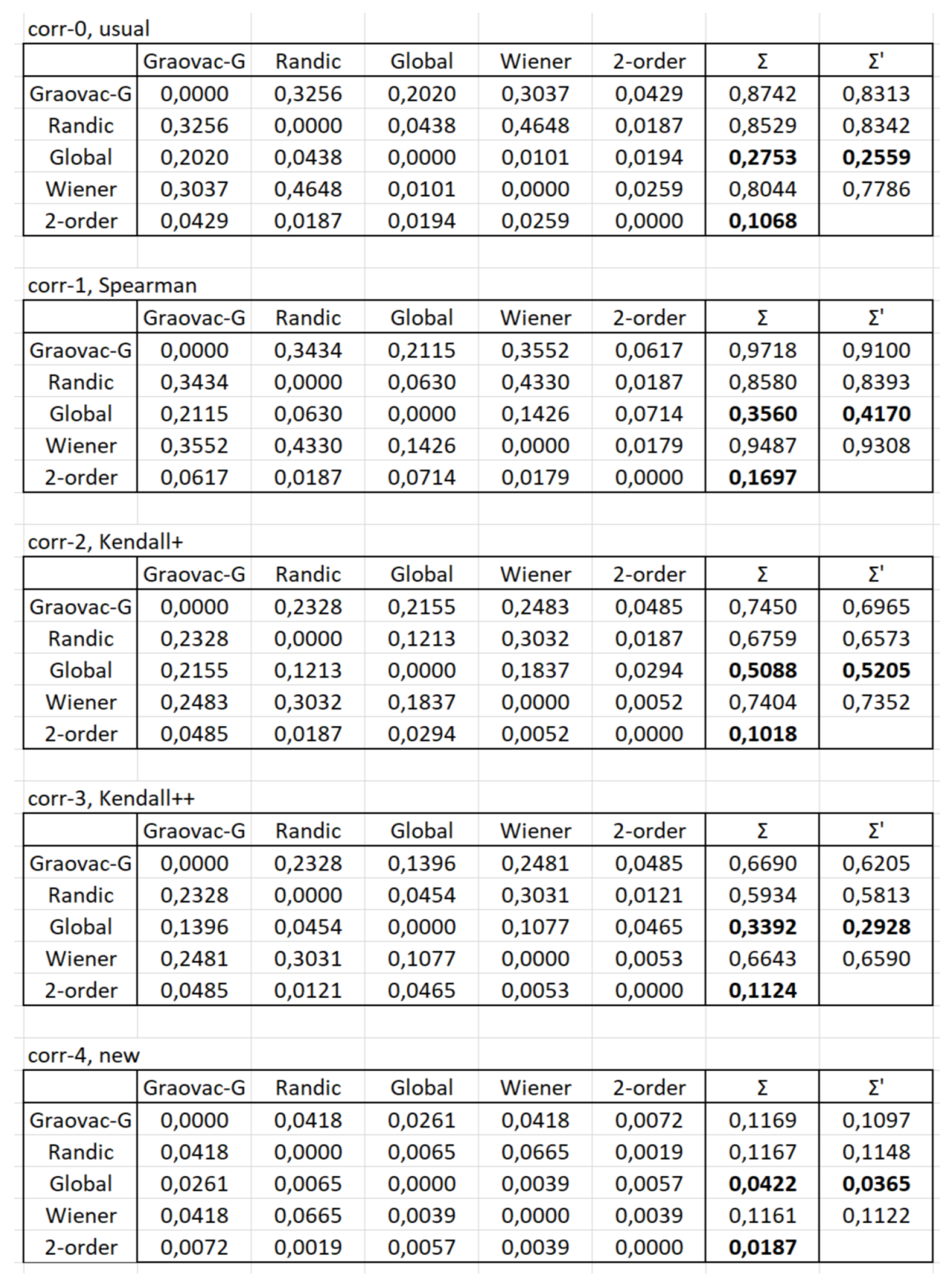
Thus, we are considering 5 options for calculating the rank correlation coefficient. For each of them, we build a table with dimension , since the number of invariants we consider is also 5. Each element of the table is equal to the value of the rank correlation for a pair of invariants corresponding to this cell of the table. For the convenience of further calculations, we fill the main diagonal with values of 0 (although in the sense there should be values of 1) 7. The sum of the values is calculated for each row (column ).
Since the authors are currently not sure that the injective mapping of a vector of second-order degrees to a number is adequately described (we believe that this needs further improvement), the sums of elements without a column corresponding to this vector of second-order degrees are calculated separately (column ).
As we expected, the ordering of the results for any of the 5 options for calculating the rank correlation coefficient is practically the same. Some surprise in the results obtained is that the vector of second-order degrees and the Randić index give completely different results (although the algorithms for these invariants are based on the same principles); however, this, of course, is far from the most significant result of calculations.
Other results obtained are of much greater interest. As we have already noted in the general description of the calculations, we believe that the small value of the sum obtained in the row indicates that such an invariant is “further” from others, i.e. it better reflects the belonging/non-belonging of some graph to the class of graphs under consideration. For each calculation method, the vector of second-order degrees turns out to be the best, and if it is excluded from consideration, the global clustering coefficients index becomes such; in each table of Figure 4, we have highlighted in bold the two best results for the first method of calculation and one best result for the second method.
9. Conclusions
Thus, we consider the main results of this paper to be the description of an approach to the study of random graphs based on their invariants and correlation coefficients between sequences of such invariants. In our opinion, this approach allows us to obtain quite a lot of results based on the proposed heuristics; we consider the following two to be the main such results.
- First, it is a heuristic that determines whether the graph in question belongs to a certain class of graphs with corresponding ranges of invariant values.
- Secondly, it is a heuristic that determines the order of consideration of invariants for various graph studies.
Both results are obtained by considering matrices containing rank correlation coefficients for sequences of invariant values.
Before formulating the most important direction for continuing the research discussed in this paper, we repeat the following. The authors really understand that we have given not the most successful (although quite possible) algorithm that forms an injective mapping of a vector of degrees of the second order into a number. In the next publication, we propose to publish an algorithm that, from our point of view, is more successful, and to present computational experiments corresponding to this algorithm.
Funding
This work was partially supported by a grant from the scientific program of Chinese universities “Program to support the stability of Higher Education” (section “Shenzhen 2022 – Commission on Science, Technology and Innovation of the Shenzhen Municipality”).
Acknowledgments
The work of the first author was partially supported by a grant from the scientific program of Chinese universities “Program to support the stability of Higher Education” (section “Shenzhen 2022 – Commission on Science, Technology and Innovation of the Shenzhen Municipality”).
Conflicts of Interest
The authors declare no conflicts of interest.
References
- R. Blanco-Rodríguez, J.N.A. Tetteh, E. Hernández-Vargas. Assessing the impacts of vaccination and viral evolution in contact networks. Scientific Reports, vol. 14, iss. 1, no. 15753 (2024). [CrossRef]
- N.-C. Yang, S.-T. Zeng, W.-Ch. Tseng. Three-phase power flow using binary tree search algorithm for unbalanced distribution networks. Electric Power Systems Research, vol. 237, no. 111019 (2024). [CrossRef]
- N. Garg, S. Singhal, N. Aggarwal, A. Sadashiva, P.K. Muduli, D. Bhowmik. Improved time complexity for spintronic oscillator ising machines compared to a popular classical optimization algorithm for the Max-Cut problem. Nanotechnology, vol. 35, iss. 4611, no. 465201 (2024). [CrossRef]
- T.A. Springer. Invariant theory. Berlin: Springer-Verlag, 1977, 120 p.
- B.F. Melnikov, E.F. Sayfullina. Applying multiheuristic approach to randomly generating graphs with a given degree sequence. News of Higher Educational Institutions. Volga Region. Physical and Mathematical Sciences, vol. 3 (27), pp. 70-83 (2013). (In Russian.). https://elibrary.ru/item.asp?id=21315166.
- E. Sayfullina. A heuristic approach to the verification of isomorphic graphs. Proc. of International Conference Information Technology and Nanotechnology, pp. 838–842 (2016). [CrossRef]
- B.F. Melnikov, E.F. Sayfullina, Y.Y. Terentyeva, N.P. Churikova. Application of algorithms for generating random graphs for investigating the reliability of communication networks. Informatization and communication, vol. 1, pp. 71-80 (2018). (In Russian.). https://elibrary.ru/item.asp?id=32651307.
- B. Melnikov, A. Samarin, Y. Terentyeva. Using Special Graph Invariants in Some Applied Network Problems. 7th Computational Methods in Systems and Software, CoMeSySo-2023, Lecture Notes in Networks and Systems, vol. 935, pp. 388–392 (2024). [CrossRef]
- M.A. Khan, K.K. Kayibi, Sh. Pirzada. Random generation of graphs with a given degree sequence. Proc. of 8th French Combinatorial Conference, University of Paris Sud, France (2010). https://www.researchgate.net/publication/276355068.
- S.M. Ergotić. On Unicyclic Graphs with Minimum Graovac–Ghorbani Index. Mathematics, vol. 12(3):384 (2024)). [CrossRef]
- I. Gutman, B. Furtula, V. Katanić. Randić index and information. AKCE International Journal of Graphs and Combinatorics, vol. 15, pp. 307–312 (2018). [CrossRef]
- R.J.M. Damalerio, R.G. Eballe, I. Jr. Serino Cabahug, Ch.M. Rivas Balingit, A.L. Ong Vicedo. Global clustering coefficient of the join and corona of graphs. Asian Research Journal of Mathematics, vol. 18, iss. 12, pp. 128–140, article no. ARJOM.95267 (2022). https://www.researchgate.net/publication/366982948.
- S. Nikolić, N. S. Nikolić, N. Trinajstić, Z. Mihalić. The Wiener index: development and applications. Croatica Chemica Acta 68(1), pp. 105-129 (1994). https://www.researchgate.net/ publication/263274230.
- B.F. Melnikov, S.V. Pivneva, M.A. Trifonov, Various algorithms, calculating distances of DNA sequences, and some computational recommendations for use such algorithms CEUR Workshop Proceedings, 1902, pp. 43–50 (2017). [CrossRef]
- B. Melnikov, M. Trenina, A. Nichiporchuk, E. Melnikova, M. Abramyan. Some new approaches to comparative evaluation of algorithms for calculating distances between genomic sequences Advances in Intelligent Systems and Computing, 1294, pp. 633–642 (2020). [CrossRef]
- P. Erdős, Graph theory and probability. Canad. J. Math., 11 (1959), 34-38. [CrossRef]
- P. Erdős, A. Rényi, On random graphs. I. Publ. Math. Debrecen, 6 (1959), 290–297. MathSciNet: 0120167.
- P. Erdős, A. Rényi, On the evolution of random graphs. Magyar Tud. Akad. Mat. Kutató Int. Közl., 5 (1960), 17–61. MathSciNet: 0125031.
- M.E. Zhukovskii, A.M. Raigorodskii. Random graphs: models and asymptotic characteristics. Russian Mathematical Surveys. 2015. vol. 70. no. 1. pp. 33–81. [CrossRef]
- M. Lagutin. Visual mathematical statistics. Moscow: Binom, 2012, 472 p. (in Russian).
- L. Wasserman. All of statistics: a concise course in statistical inference. Berlin: Springer Science & Business Media, 2013. 442 p.
- B.F. Melnikov, A.A. Melnikova. Edge-minimization of non-deterministic finite automata. The Korean Journal of Computational and Applied Mathematics (Journal of Applied Mathematics and Computing), 2001, vol. 8, no. 3, pp. 469–479.
- B.F. Melnikov, A.A. Melnikova. Some properties of the basis finite automaton The Korean Journal of Computational and Applied Mathematics (Journal of Applied Mathematics and Computing), 2002, vol. 9, no. 1, pp. 135–150.
| 1 |
In these papers, among other things, we compared the descriptive capabilities of the Randić index and the vector of second-order degrees, while also gaining the advantage of the vector; regarding the material of these articles, it is important to note the following.
|
| 2 | At the same time, of course, do not confuse the numbers of invariants (we use 5 items) with the numbers of variants of the correlation coefficient (we shall also use 5 items, see below). |
| 3 | 10 counting options are obtained as follows: we have 5 options for calculating rank correlation; for each of them, we can use either all 5 graph invariants or not use a vector of second-order degrees. |
| 4 |
To the basic idea formulated before, let us note the following.
|
| 5 | It is clear that there are other natural ways to arrange the vertices of a second-order vector, and they can be used in some other tasks. It is convenient for us to apply exactly the described method. |
| 6 | We should immediately note that the correlation calculated in any way between the usual Kendall’s correlation coefficient and our variant is always equal to 1 (“correlation between correlations”), this is easily obtained by trivially considering the formulas. |
| 7 | A complete analogy can be seen in the fact that when solving the traveling salesman problem by the method of branches and boundaries, it is convenient to set infinity values (∞) on the main diagonal of the matrix (although in the sense there should be values of 0). |
Figure 1.
The example of the graph with the number of vertices adjacent to each one
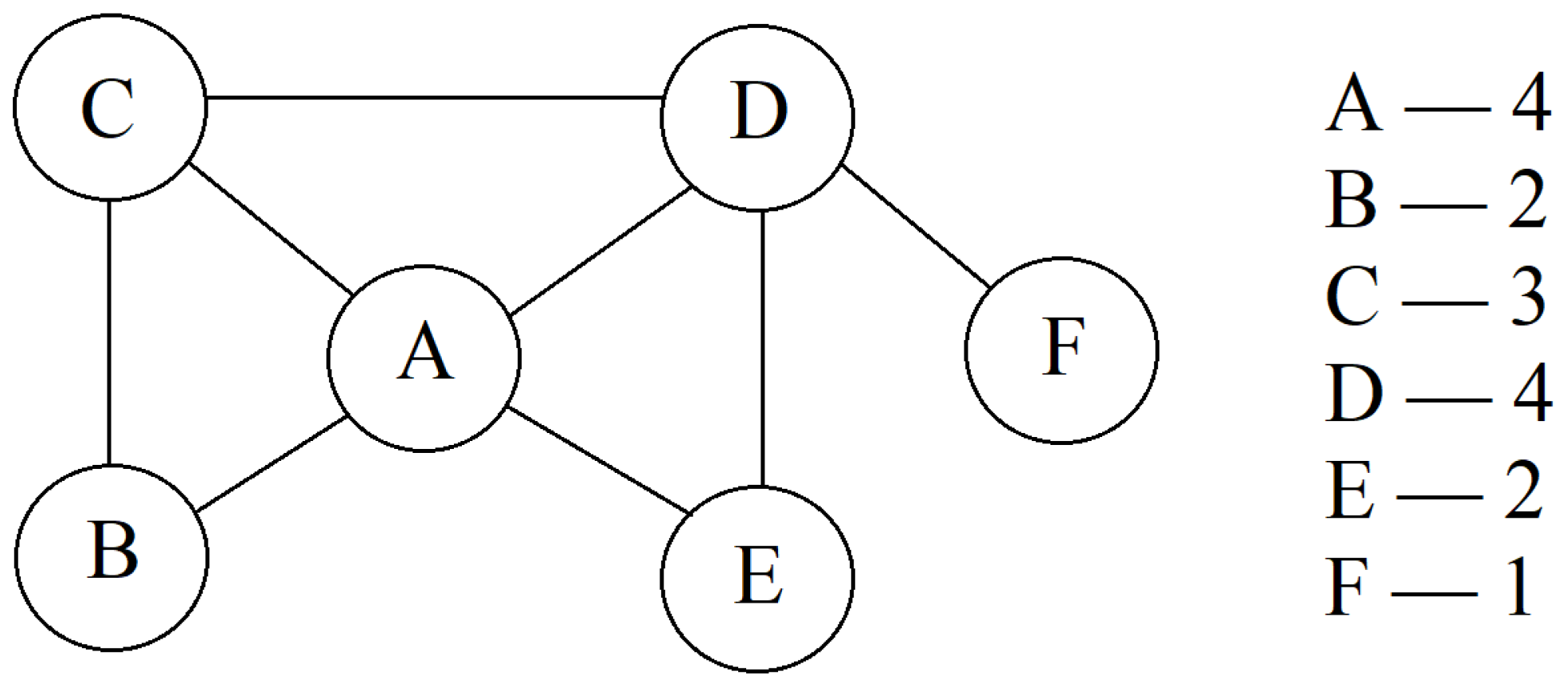
Figure 2.
The simple example of the graph with the number of vertices adjacent to each one
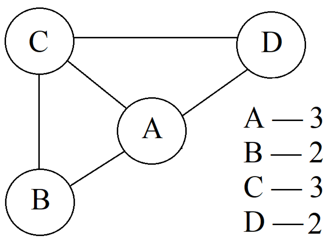
Figure 3.
The proposed calculation of the pair correlation
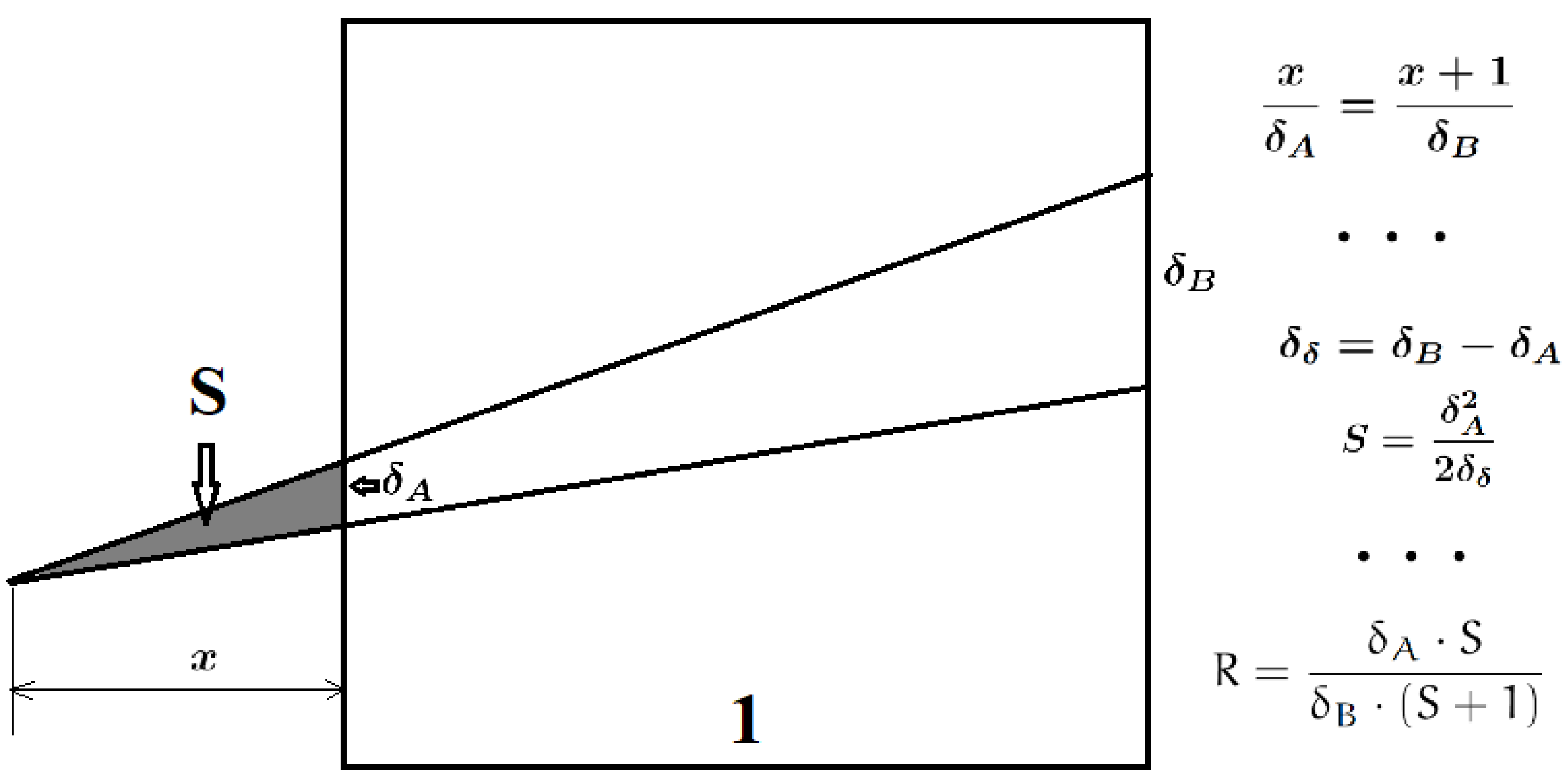
Figure 4.
The main results of calculations
Disclaimer/Publisher’s Note: The statements, opinions and data contained in all publications are solely those of the individual author(s) and contributor(s) and not of MDPI and/or the editor(s). MDPI and/or the editor(s) disclaim responsibility for any injury to people or property resulting from any ideas, methods, instructions or products referred to in the content. |
© 2025 by the authors. Licensee MDPI, Basel, Switzerland. This article is an open access article distributed under the terms and conditions of the Creative Commons Attribution (CC BY) license (http://creativecommons.org/licenses/by/4.0/).
Copyright: This open access article is published under a Creative Commons CC BY 4.0 license, which permit the free download, distribution, and reuse, provided that the author and preprint are cited in any reuse.


