
Submitted:
01 April 2025
Posted:
01 April 2025
You are already at the latest version
Abstract
We compare the “classical” equations of type-token systems, namely Zipf’s laws, Heaps’ law and the relationships between their indices, with data selected from the Standardized Project Gutenberg Corpus (SPGC). Selected items all exceed 100,000 word-tokens and are trimmed to 100,000 word-tokens each. With the most egregious anomalies removed, a dataset of 8,432 items is examined in terms of the relationships between the Zipf and Heaps indices computed using the Maximum Likelihood algorithm. Zipf’s second (size) law indices suggest that the types vs. frequency distribution is log-log convex, the high and low frequency indices showing weak but significant negative correlation. Under certain circumstances the classical equations work tolerably well, though the level of agreement depends heavily on the type of literature and the language (Finnish being notably anomalous). The frequency vs. rank characteristics exhibit log-log linearity in the “middle range” (ranks 100-1000), as characterized by the Kolmogorov-Smirnoff significance. For most items, the Heaps’ index correlates strongly with the low-frequency Zipf index in a manner consistent with classical theory, while the high frequency indices are largely uncorrelated. This is consistent with a simple simulation.
Keywords:
language statistics
; Zipf’s laws
; Heaps’ law
1. Introduction
Type-token systems consist of “types” of object, whose individual occurrences are referred to as “tokens”. In a biological habitat, types might represent species and tokens individual organisms [1,2]. Type-token models have been applied to galactic superclusters [3], the popularity of musical works [4], the sizes of software components [5] and the statistics of written and spoken texts (including dialogues) [6]. In the latter case, unique lexical units (lemmas, wordforms, bi- or trigrams) form types and their specific instances form tokens. The early work of Zipf [7,8], Mandelbrot [9] and Simon [10] have identified underlying power laws, especially the two laws of Zipf and Heaps’ law, whose exponents are supposedly linked by a series of mathematical relationships. We shall call this the “classical model”.
Here we compare this classical model with data extracted from the Standardized Project Gutenberg Corpus (SPGS) [11], which comprises nearly 60,000 works of literature, mostly English, spanning many genres and historical periods. For the purposes of this work, we define types as complete wordforms, regardless of common stems. It thus extends our two earlier two papers [12,13] with a larger and more consistent dataset and demonstrates the ranges of applicability of the classical equations.
2. The Classical Model
Although Zipf’s first law (the “types” law) was named for George Kingsley Zipf following his famous treatise of 1948 [8], it was known at least 35 years before this when it was observed in the distribution of city-sizes [14]. It links the frequency of a type to its “rank” ( being the most frequent type, the second most frequent etc.):
Where (the “Zipf alpha index”) is typically in the region of 1. Figure 1 shows the log-log frequency vs. rank distributions for two typical English texts, showing that changes significantly between different ranges of . Nevertheless, both exhibit a “middle range” () over which α is approximately constant. The reduced log-log slope for small is embraced by the Zipf-Mandelbrot law [9] where is an additional constant, which is asymptotically equivalent to (1) when .
If word type selection were statically independent, with a probability distribution , normalization would require that at the upper extremity of , though may exist in other regions. Indeed, from an aggregate frequency/rank plot of over 2,606 English books, Montemurro [15] observed for , an effect also seen in the BNC corpus [16] and the Gutenberg corpus for [17]. It has been suggested that the switchover between low and high domains may correspond to the transition from a common kernel lexicon to vocabularies used for specific communications; the latter limited only by the capacity of the human brain [16]. The graphs of Figure 1 relate to individual 100,000-word texts, where discrete plateaux in their upper tails (representing … etc. [18]) are difficult to interpret in terms of (1). However, there is a strong suggestion of downward “droop” and hence increasing with increasing .
Zipf’s second (or “size”) law relates the token frequency to the number of types exhibiting that frequency (i.e. the widths of the low frequency plateaux in Figure 1):
where the , the “Zipf beta index”, is typically between 1 and 2. Like the first law, it predates Zipf’s work and was noted by Corbet in a 1941 a study of Malayan lepidoptera [19]. Figure 2 shows Corbet’s data, indicating across , an abnormally low value compared with that of the more typical distribution of the King James Bible also shown (). Simon [10] noted that for both words and biological genera, (), comprising approximately half the token population. We note from Figure 2 that while the log-log slopes are approximately constant at low frequencies, extrapolating the law for mostly overestimates the data, suggesting a general log-log convexity or an increasing with increasing frequency. Many authors talk of a“low frequency cut-off (the law only valid for ), estimated 6, 8 and 51 for different English novels [20]. In view of this, one might suppose that Zipf’s second law is only truly valid in the noisy discretized part of the graph, and the seemingly smooth section is in fact the anomaly.
The third power relationship is Heaps’ (or Herdan’s) law, which is an observed sublinear increase in the total number of types as the total number of tokens t increases [21]
where the constant , the “Heaps index”, lies between zero and one. Figure 3 shows how this law holds roughly across at least two decades for two randomly selected documents (one English, the other Finnish).
Although an unbounded increase (both of hapaxes and total types) suggests an infinite accessible vocabulary, this cannot literally be true: a 20-year-old English speaker knows approximately 42,000-word lemmas [22] while the OED of 2020 has 171,476 [13]. Estimating that English lemmas have around four common variations and allowing for proper names and spelling alternatives, the maximum English vocabulary could contain around a million unique wordforms. However, no English text even approaches this: the entire King James Bible has only 12,143 unique wordforms and the aggregate corpus analyzed by Montemurro [15] contains no more than 448,359. The latter comprises 2,626 volumes, each with its own unique jargon and terminology; one cannot suppose that this comes close to exhausting all possible wordforms, especially as language constantly evolves with the introduction of new words (neologisms). Despite this, vs. saturation is seen in ideogrammic languages like Chinese where the dictionary of semantic characters does have a finite limit [23].
It is often claimed (e.g. [24]) that (2) and (3) are inevitable consequences of (1) with the two indices inextricably related
Similar relationships exist between the Zipf and Heaps indices:
and the Zipf and Heaps indices:
Under certain assumptions and approximations, these equations are reasonably self-consistent. Lü et al. [25] (amongst others) take (1) as the most fundamental law, describing the selection probability for different types, each characterized by an underlying “rank” (not necessarily its rank within any given sample). If this is approximated by a continuous probability density function
(where is a constant) then the frequency range associated with a small number of contiguous ranks is given by
Solving (7) for and substituting into (8) gives , which approximates the number of types (ranks) associated with a single frequency (). We thus obtain expressions (2) and (4). Some workers (e.g. [3,26]) have taken the opposite approach, making (2) the fundamental law and inferring (1) and (4), though the analysis is largely equivalent. As for Heaps’ law (3), several quite rigorous proofs exist (e.g. [27]) but the following provides a useful intuition [25]: loosely interpreting as the rank at which , we note that (1) can be rewritten . Since the token population must be approximately the integral of this function across we find that
Although this is not analytically solvable for , if then which gives (3) and (5). Finally (6) is obtained by a simple substitution of (5) into (4).
The most glaring assumption so far is that the continuous probability distribution (7) provides an adequate approximation for what is actually a discrete stochastic process. Discrete analysis based on fixed and unlimited word types [28] shows that although (3) and (5) are valid, (2) and (4) are asymptotically true only for large [13,29]. At smaller frequencies, is predicted to increase with decreasing , contradicting a general observation that decreases slightly as approaches 1 [13] (mirroring the low frequency “droop” observed in Figure 1). This effect can be duplicated in the model by imposing an upper limit on the number of accessible types (a “closed vocabulary”), but this is clearly an artificial “fudge” [13]. Furthermore, when this model is optimised to fit a random selection of texts, the resulting low frequency exhibits a greater variability than the corresponding directly measured value. When extended beyond the sample to which it was optimised, the model must inevitably predict a rapid decrease in the numbers of low-ranking types as potential new word-types are exhausted. This clearly contradicts the common observation that the numbers of hapax legomena (types represented by only one token) always increase without saturation, as required by Heaps’ law.
A second assumption is that word selection is an independent random process governed by a statical probability distribution. Common sense tells us this cannot be true, since the sample space for each successive word is generally dictated by its predecessors [30]. There are also empirical reasons to be suspicious: during population growth, observed ranks change much more frequently than the model would predict, and their relative frequencies do not always converge towards stable values [24]. Tria et al. [17] point out that (5) is only true under random word selection when , and would require .
There have been many attempts to develop all three laws from an underlying dynamical framework in which the type-selection probability is not static (e.g. [26,31]). These are mostly variants of the Pólya urn model, in which the probability of a type’s future selection increases in proportion to its past selection; the so-called “rich get richer” principle. As early as 1955 Simon [10] showed that if the selection probability of a word type with frequency is proportional to , and the generation probability of new word types is constant, then an approximation to Zipf’s second law emerges. This idea has been developed and expanded over several decades, recently by Tria et al. [17] who suggested that the appearance of a new type triggers expansion into an “adjacent possible”, introducing further types not hitherto accessible.
We note these models for the sake of completeness but do not attempt to expand upon them in this paper. We concentrate instead on the equations themselves and their relationship with observation.
3. Materials and Methods
As previously noted, and are not a truly constant but vary between different sections of their respective distributions. To investigate the variation of with frequency we define the seven frequency ranges shown in Figure 4, overlaid upon a typical size/frequency distribution (the Project Gutenberg item PG10, the King James Bible). While the log-log slope over Range 1 (frequencies 1-10) is clearly perceived, the same cannot be said of Range 7 (frequencies 64-640) where the underlying continuous curve is obscured by discretization and random noise. Nevertheless, the Maximum Likelihood (ML) method [32] gives optimum for Ranges 1 to 7 respectively. Previous observations (see Section 2) suggest a degree of log-log convexity, meaning that (2) will not be strictly valid even within an individual range: nevertheless, if we assume that it is approximately valid then the optimized may be considered representative of range and compared with the values obtained for other ranges.
The following procedure is used to select a “clean” subset of this SPGC, allowing general statistics to be studied with minimal disturbance from unrepresentative and anomalous phenomena.
1. To eliminate document length as an interfering variable, all items with less than 100,000 word tokens are rejected. The remainder are trimmed to exactly 100,000 tokens each.
2. The item PG4656 “Checkmates for Four Pieces” by W.B. Fishburne is removed. (This consists almost entirely of chess notation, which is not amenable to iterative process of optimizing maximum likelihood).
3. While most of the remaining data follow a clear “main sequence” (a term we borrow from star classification [33]), anomalies still exist in the data. To classify these anomalies consistently we define where is a Gaussian “support” function with standard deviation and is the Zipf index computed for item over the frequency range ( in this case being 7). For item , the average support from the other items , where is the total number of items.
4. If (where is some arbitrary threshold) then item is classified as anomalous.
Figure 5 shows the cumulative distribution of for four possible values of . The classification clearly depends on as well as , and while the choice is ultimately subjective, we use since it creates a clear dichotomy at .
Of the 57,713-item SPGC, approximately 16% survive this winnowing process and are included in our main study. Table 1 lists the seven anomalies identified in stage 3, along with the seven highest-scoring items.
Figure 6 shows some example plots of for different frequency ranges. We note that while some anomalies appear close to the non-anomalous data, this is an illusion of perspective in 7-dimensional space; the rightmost column of Table 1 shows the shortest Euclidean distance of any anomaly to its nearest neighbour is 0.594, while for the seven highest scoring items this is at least an order of magnitude lower.
This procedure only removes anomalies manifested in the -data, when the full 100,000 tokens of each item are analyzed. Remaining anomalies appearing in the and indices are considered as and when they arise.
4. Observations on the Zipf Indices
Figure 7(a) shows the resulting mean values of together with the corresponding upper and lower quartiles. While statistical variation is large, the mean shows a gradually slowing increase with increasing frequency, peaking at a little under 2 before falling very slightly at the highest range 7. This agrees with the long-established log-log convexity of vs. , being smallest for the smallest frequencies (though never becoming negative as a closed vocabulary model would require [13]). Figure 6(b) shows the corresponding KS-significance [34], a measure of how plausibly the distributions follow the power law (1 being the most plausible and 0 the least). Median values and upper and lower quartiles are also shown. Note that when the frequency is low, the median is at 0.7 with an almost maximal interquartile range. As frequency increases, the median rises to a maximum of about 0.9 while the interquartile range narrows. For higher frequencies still, the median falls very slightly with a steady interquartile range; we may suppose that in this region most items are above the “low frequency cut-off” (as defined by Corral et al. [20]). For the combined range 1-640 (ranges 1-7 combined) only 10% of items have KS-significance exceeding 0.01, and the interquartile range cannot meaningfully be plotted on this scale. Zipf’s second law is therefore approximately valid across the individual ranges but generally does not apply across the entire range of frequencies.
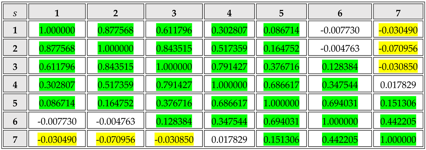
Table 2 shows a matrix of the Pearson correlation coefficients between -values computed across different frequency ranges: adjacent (overlapping) ranges have a strong positive correlation, while those far apart show a very weak negative correlation. For example, a higher than average tends accompany a lower than average , which suggests that that beneath the noise, size/frequency distributions differ not so much in their absolute slopes but in their respective log-log convexities.
5. Zipf Indices in the Middle Range
It has long been recognized that Zipf’s frequency/rank law is most accurate in the “middle range”, with major deviations appearing for high and low ranks [24]. However, it is by no means obvious where the boundaries of this “middle range” lie, nor whether a common definition can be applied to different items. Qualitative examination suggests that many items have an approximately log-log linear range (characterizable by a constant between ranks 100 and 1000, although many exceptions can be found. We therefore apply the Kolmogorov-Smirnov (KS) test [34] to the ML frequency vs. rank best-fits for ranks 100-1000, for all the non-anomalous items identified in Section 2. Figure 8 shows the cumulative distribution of KS-significance, along with highlighted items whose frequency/rank distributions are shown in Figure 9. We see that for KS significances greater than about 0.01 the graph has tolerable log-log linearity, whereas lower KS values are indicative of an increasing log-log convexity.
Somewhat arbitrarily (based on a qualitative assessment of “what looks right”) we choose a boundary value of 0.03 to classify items into “low” and “high” KS-significance groups, the former comprising the lowest decile. Figure 10 shows the cumulative distributions for mid-range for these two groups, indicating that the low KS-significance -values are on average significantly higher than those of the low KS-significance group. (We recognise however that -values obtained with a low KS-significance may not be entirely meaningful, since linear spacing of ranks creates a bias towards the upper end of the middle range, where the log-log slope is higher.)
6. Alpha vs. Beta
Figure 11, Figure 12, Figure 13, Figure 14, Figure 15, Figure 16 and Figure 17 show the indices plotted against the corresponding mid-range for low and high KS significance items, along with the theoretical curve predicted by (4). The cumulative distributions of are also shown. Figure 18 summarizes the correlation coefficient magnitudes for all seven graphs. Our initial qualitative observations are as follows:
1. For the low frequency ranges the correlation coefficient magnitude is very low. It rises close to unity for range 6, where the frequencies correspond roughly to the middle range ranks across which was computed. It then falls again in range 7. (See Figure 18).
2. Agreement with (4) generally improves as the frequencies increase, the best fit being for Range 5 (Figure 15). Here items with higher KS-significance are distributed almost symmetrically around the theoretical line, while items with lower KS-significance exist in separate clusters above and below. There is a hint of this behaviour for ranges 4 and 7, though it is curiously it is absent for range 6 (Figure 16).
3. Throughout all frequency ranges there is a clear difference between the mean for high and low KS-significance. While in the low frequency ranges, low KS-significance items have a lower average , the difference narrows with increasing frequency. The difference eventually reverses for range 7 (Figure 17), though here there is an intersection of the two cumulative distributions created by the clustering above and below the model.
4. For range 1 (and to some extent 2) there is a distinct cluster of high- points, also characterized by a narrower -range than the main population. These points are numerically quite close to the theoretical curve, though they show no obvious indication of following it. Nearly all these items belong to the high KS-significance group and nearly all of them are Finnish; we therefore refer to this feature as the “Finnish cluster”. (The main cluster centred around is dominated by English items.)
5. For range 5 there is a distinct “filament” of data points exhibiting low , all of which belong to the low KS-significance group.
6.1. The “Finnish Cluster”
Figure 11 shows a prominent cluster of high items, nearly all of which are Finnish, which belong exclusively to the high KS-significance group. (Finnish items do not appear anywhere else in this graph.) For analytical purposes, we define this cluster as containing all items whose indices fall within the rectangle , (shown on Figure 10) and plot the cluster size as a function of a KS-significance limit between 0.01 and 1 (see Figure 19). We find the cluster only exists for KS-significances above 0.048, beyond which its relative size increases approximately linearly with the increasing logarithm of the KS-significance.
Comparison between the Finnish cluster and the main (mostly English) population suggests significant differences between the statistical properties of languages. English is well known for its limited inflexion and agglutination, while Finnish is heavily agglutinated and inflected (more so even than German), giving it a much larger variety of wordforms. Our results also suggest that compared to English, Finnish has a closer adherence to Zipf’s first law (evidenced by the high KS-significance) and a significantly higher -index for lower frequencies. We intend to investigate this further, along with the statistical differences between other languages.
6.2. The Middle Range and the “Low Beta Filament”
Here we examine the filament of low , low KS-significance data points seen in Figure 15 (and to a lesser extent 16). In this range the frequencies correspond most closely to the middle range of ranks across which the -indices were measured. This is evidenced by the close adherence (at least amongst the high KS-significance data) to the model (4). To obtain a more precise correspondence we calculate the average upper and lower frequencies corresponding to the ranks 100 and 1000 across the entire dataset and Figure 20(a) and (b) show the values recomputed for this range. The “low beta filament” is visible in Figure 20(a), though maybe not quite so clearly as in Figure 15. This filament comprises items of the lowest KS-significance, including those less than highlighted in Figure 20(c). It includes many editions of the CIA World Factbook and other works of reference. Meanwhile the highest KS-significant data in Figure 20(d) are those in closest agreement with (4).
7. Vocabulary Growth and Heaps’ Law
So far we have applied Zipf’s first and second laws to documents with a fixed length of 100,000 word tokens. Meanwhile Heaps’ law (3) describes the growth of documents and is theoretically linked to Zipf’s laws by (5) and (6). An optimum Heaps’ index was obtained for each item by iteratively adjusting to minimize the mean square difference between (3) and the measured vocabulary profile across 100 intervals of 1000 tokens each. Figure 21 shows the cumulative frequency distributions for optimized Heaps’ indices obtained for items with high and low KS-significance. Our first observation is that for the low KS-significant items, the average Heaps index is significantly lower than for the high KS-significant items, with a larger standard deviation.
Figure 22, Figure 23, Figure 24, Figure 25, Figure 26, Figure 27 and Figure 28 show plotted against the indices for the seven frequency ranges, compared with the prediction of (6). (We again separate items into the high and low KS-significance groups.) For range 1 (Figure 22) the data in both groups are strongly correlated. The bulk of points agree roughly with the theoretical curve (6), although items in the “Finnish cluster” (which have a considerably higher than average ) lie well above the theoretical prediction. Figure 29 summarises the correlation coefficients. As the frequencies increase, the correlation coefficient falls as correspondence with (6) is gradually lost. This makes sense, since is associated with the rate at which new types (types with frequency 1) appear and would be mostly associated with the lowest frequency statistics.
However, vocabulary growth is also retarded by the reappearance of existing types, so one would expect some correlation with higher frequency statistics. To investigate this, we propose a simplified model to represent the frequency-rank distribution and obtain the corresponding profile of vocabulary growth. To represent the imperfect adherence to Zipf’s first law we propose an -value which changes abruptly at some rank , from a high-frequency value to a low-frequency value :
Following (4) we define high and low frequency indices, and respectively. Log-log convexity requires that so .
Since high- and low-frequency have no meaningful correlation (see Table 2) we generate and as independent Gaussian random variables. Substituting (10) into (9) we obtain the corresponding expression for the token population :
allowing to be computed iteratively for any value of . From the profile of vs. (using 100 steps of 1000 tokens) optimal values of obtained by minimizing the mean square error. While this model is not precise, it nevertheless provides an insight into the observed behaviour of real texts. We generate values of and with means 1.9 and 1.6 respectively (corresponding roughly to the middle values in Figure 11 and Figure 17), with both standard deviations set to 0.15. Combinations for which are rejected and recomputed to ensure a minimum degree of log-log convexity. The transitional rank is set to 1000, to correspond with the upper limit of the middle range as defined in Section 5.
Figure 30 shows scattergrams of (a) and (b) plotted against the optimised Heaps index : while the latter shows little correlation with (as in the experiment), the former is strongly correlated and approximately follows (6) (though deviating somewhat for large ). Statistical scatter is far less than observed in Figure 22, though this is to be expected with a simplified model with far fewer variables than the reality. The parallelism between the base of the data clusters in Figure 25 and Figure 26 is reproduced in Figure 30(b) where it is clearly related to log-log convexity (i.e. ; note that if then (11) would become identical to (9) and all points would lie on the theoretical line).
8. Discussions and Conclusions
This paper examines the agreement between data taken from the Standardized Project Gutenberg Corpus (SPGC) and the classical type-token equations used by (amongst many others) Kornai [24] and Lü et al. [25]. Items selected for study are all truncated to exactly 100,000 word tokens, and the Zipf indices are computed across seven logarithmically frequency ranges. Outliers are identified in terms of their proximity to other data-points by means of a Gaussian support function and eliminated from the main study. Our findings can be summarised as follows.
1. Outlying items identified in the -data are all dictionaries, while items with the highest support are dominated by religious works.
2. Although wide statistical variations exist, the average index generally increases with increasing frequency, corresponding to a log-log convexity of the types vs. frequency distribution.
3. The indices measured for closely overlapping frequency ranges show a strong positive correlation, while those for frequency ranges widely separated show a weak negative correlation. (For example, if is above average in the frequency range 1 to 10, then it is likely to be below average in the range 64-640,)
4. Adherence to Zipf’s first law across the middle range (defined as the interval between ranks 100 to 1000 inclusive) may be characterised by the Kolmogorov-Smirnoff (KS) significance. Items with a high KS-significance in this region tend to have a slightly lower Zipf index and a higher index across all but the highest frequency range.
5. When the frequency range used to compute corresponds roughly to the previously defined middle range (Figure 15), the points roughly follow the classical equation (4). Of these, items with the highest KS-significance follow the equation most closely (Figure 20).
6. Two notably anomalous phenomena appear in the plots of vs. . Firstly, for range 1 (frequencies 1 to 10) there exists a distinct secondary cluster of points, all with high and all of which have high KS-significance (>0.048). Nearly all of these are Finnish. Secondly for frequencies corresponding to the middle range we note a “filament” of low- points, all of which have especially low KS-significance (). All of the latter are reference books.
7. For the lowest frequency range, the index correlates strongly with the optimised Heaps index in a manner roughly consistent with the equation (6). (The Finnish items noted in point 6 are an exception.) This correlation gradually disappears as the frequencies increase.
8. A simplified model based upon an abrupt change in and between high and low frequencies (to create a convex distribution) reproduces the basic features observed in the data. We note that the Heaps’ index is largely dependent on the statistics of the lowest-frequency types and is affected only weakly by the high-frequency indices.
While all these points merit further study, we are particularly fascinated by the dichotomy between the Finnish items and the main body of data. We are furthermore interested to discover if other languages have similar peculiarities and what mathematical models can be used to describe their behaviour. The SPGC has a paucity of Finnish: our selection (based on document length and -statistics alone) contains only 165 Finnish items, compared to 7,932 items in English. We therefore intend to compile a much larger corpus of items in Finnish and other languages in order to investigate further.
Author Contributions
Conceptualization, M.T.; methodology, M.T.; software, M.T.; validation, M.T.; formal analysis, M.T and G.H.; investigation, M.T.; resources, M.T.; data curation, M.T.; writing—original draft preparation, M.T.; writing—review and editing, M.T. and G.H.; visualization, M.T..; supervision, G.H.; project administration, M.T.; All authors have read and agreed to the published version of the manuscript.
References
- Mora, C.; Tittensor, D.P.; Adl, S.; Simpson, A.G.B.; Worm, B. How Many Species are there on Earth and in the Ocean? PLoS Biology 2011, 9, e1001127. [Google Scholar] [CrossRef] [PubMed]
- Costello, M.J.; Wilson, S.; Houlding, B. Predicting Total Global Species Richness Using Rates of Species Description and Estimates of Taxonomic Effort. Syst. Biol. 2011, 61, 871–871. [Google Scholar] [CrossRef] [PubMed]
- de Marzo, G.; Labini, D.; Pietronero, L. Zipf's Law for Cosmic Structures: How Large are the Greatest Structures in the Universe? Astronomy and Astrophysics 2021, 651, A114. [Google Scholar] [CrossRef]
- Dodd, J.; Letts, P. Types, Tokens, and Talk about Musical Works. Journal of Aesthetics and Art Criticism 2017, 75, 249–1963. [Google Scholar] [CrossRef]
- Hatton, L. Power-Law Distributions of Component Size in General Software Systems. IEEE Trans. Softw. Eng. 2008, 35, 566–572. [Google Scholar] [CrossRef]
- Linders, G.; Louwerse, M. Zipf's Law Revisited: Spoken Dialog, Linguistic Units, Parameters and the Princip. Psychonomic Bulletin & Review 2023, 30, 77–101. [Google Scholar]
- Zipf, G. The Unity of Nature, Least-Action, and Natural Social Science. Sociometry 1942, 5, 48–62. [Google Scholar] [CrossRef]
- Florence, P.S.; Zipf, G.K. Human Behaviour and the Principle of Least Effort. Econ. J. 1950, 60, 808. [Google Scholar] [CrossRef]
- Mandelbrot, B. An informational theory of the statistical structure of language. In Communication Theory,; Jackson, W., Ed.; Butterworths Scientific Publications: London, 1953; pp. 486–502. [Google Scholar]
- Simon, H.A. On a Class of Skew Distribution Functions. Biometrika 1955, 42, 425–440. [Google Scholar] [CrossRef]
- Gerlach, M.; Fon-Clos, F. A Standardized Project Gutenberg Corpus for Statistical Analysis of Natural Language and Quantitative Linguistics. Entropy 2020, 22, 126. [Google Scholar] [CrossRef]
- Tunnicliffe, M.; Hunter, G. The predictive capabilities of mathematical models for the type-token relationship in English language corpora. Comput. Speech Lang. 2021, 70, 101227. [Google Scholar] [CrossRef]
- Tunnicliffe, M.; Hunter, G. Random sampling of the Zipf–Mandelbrot distribution as a representation of vocabulary growth. Phys. A: Stat. Mech. its Appl. 2022, 608. [Google Scholar] [CrossRef]
- Auerbach, F. The Law of Population Concentration. EPB: Urban Analytics and City Science 2023, 50, 290–298. [Google Scholar] [CrossRef]
- Montemurro, M.A. Beyond the Zipf–Mandelbrot law in quantitative linguistics. Phys. A: Stat. Mech. its Appl. 2001, 300, 567–578. [Google Scholar] [CrossRef]
- Ferrer-i-Cancho, R.; Sole, R. Two Regimes in the Frequency of Words and the Origin of Complex Lexicons: Zipf's Law Revisited. Journal of Quantitative Linguistics 2001, 8, 165–173. [Google Scholar] [CrossRef]
- Tria, F.; Loreto, V.; Servedio, V.D.P. Zipf’s, Heaps’ and Taylor’s Laws are Determined by the Expansion into the Adjacent Possible. Entropy 2018, 20, 752. [Google Scholar] [CrossRef] [PubMed]
- Bolea, S.C.; Pirnau, M.; Bejinariu, S.-I.; Apopei, V.; Gifu, D.; Teodorescu, H.-N. Some Properties of Zipf’s Law and Applications. Axioms 2024, 13, 146. [Google Scholar] [CrossRef]
- Corbet, S.A. The Distribution of Butterflies in the Malay Peninsula (Lepid.). Proc. R. Ent. Soc. Lond. (A) 1941, 16, 101–116. [Google Scholar] [CrossRef]
- Corral, Á.; Boleda, G.; Ferrer-I-Cancho, R. Zipf’s Law for Word Frequencies: Word Forms versus Lemmas in Long Texts. PLOS ONE 2015, 10, e0129031. [Google Scholar] [CrossRef]
- Ross, A.S.C.; Herdan, G. Type-Token Mathematics: A Textbook of Mathematical Linguistics. J. R. Stat. Soc. Ser. A (General) 1960, 123, 341. [Google Scholar] [CrossRef]
- Brysbaert, M.; Stevens, M.; Mandera, P.; Keuleers, E. How Many Words Do We Know? Practical Estimates of Vocabulary Size Dependent on Word Definition, the Degree of Language Input and the Participant’s Age. Front. Psychol. 2016, 7, 1116. [Google Scholar] [CrossRef] [PubMed]
- Kornai, A. How Many Words Are There? Glottometrics 2002, 4, 61–86. [Google Scholar]
- Kornai, A. Zipf’s Law Outside the Middle Range, in 6th Meeting on Mathematics of Language, 1999, University of Central Florida.
- Lü, L.; Zhang, Z.-K.; Zhou, T. Zipf's Law Leads to Heaps' Law: Analyzing Their Relation in Finite-Size Systems. PLOS ONE 2010, 5, e14139. [Google Scholar] [CrossRef]
- De Marzo, G.; Gabrielli, A.; Zaccaria, A.; Pietronero, L. Dynamical approach to Zipf's law. Phys. Rev. Res. 2021, 3, 013084. [Google Scholar] [CrossRef]
- van Leijenhorst, D.; van der Weide, T. A Formal Derivation of Heaps' Law. Information Sciences 2005, 170, 263–272. [Google Scholar] [CrossRef]
- Mandelbrot, B. On the Theory of Word Frequencies and on Related Markovian Models of Discourse. In Structure of Language and its Mathematical Aspects; Jakobson, R., Ed.; American Mathematical Society: Rhode Island, 1961; pp. 190–219. [Google Scholar]
- Corral, Á.; Serra, I.; Ferrer-I-Cancho, R. Distinct flavors of Zipf's law and its maximum likelihood fitting: Rank-size and size-distribution representations. Phys. Rev. E 2020, 102, 052113. [Google Scholar] [CrossRef]
- Thurner, S.; Hanel, R.; Liu, B.; Corominas-Murtra, B. Understanding Zipf's law of word frequencies through sample-space collapse in sentence formation. J. R. Soc. Interface 2015, 12, 20150330. [Google Scholar] [CrossRef]
- Zanette, D.; Montemurro, M. Dynamics of Text Generation with Realistic Zipf's Distribution. J. Quant. Linguistics 2005, 12, 29–40. [Google Scholar] [CrossRef]
- Bauke, H. Parameter estimation for power-law distributions by maximum likelihood methods. Eur. Phys. J. B 2007, 58, 167–173. [Google Scholar] [CrossRef]
- ANTF. The Hertzsprung-Russell Diagram, Commonwealth Scientific and Industrial Research Organization, n.d. [Online]. Available: https://www.atnf.csiro.au/outreach/education/senior/astrophysics/stellarevolution_hrintro.html. (Accessed 15 July 2024).
- Press, W.H.; Teukolsky, S.A.; Vetterling, W.T.; Flannery, B.P. Numerical Recipes in C: The Art of Scientific Computing (2nd. Ed.); Cambridge University Press, 1992. [Google Scholar]
Figure 1.
Frequency vs. rank for two typical English texts. While the log-log slope varies between different ranges of , it remains approximately constant in the “middle range” () where it is marginally greater than unity. For ranks above the middle range, each graph discretizes into a series of plateaux, each representing a particular value of . Both graphs suggest the beginnings of a downward “droop” in this region.
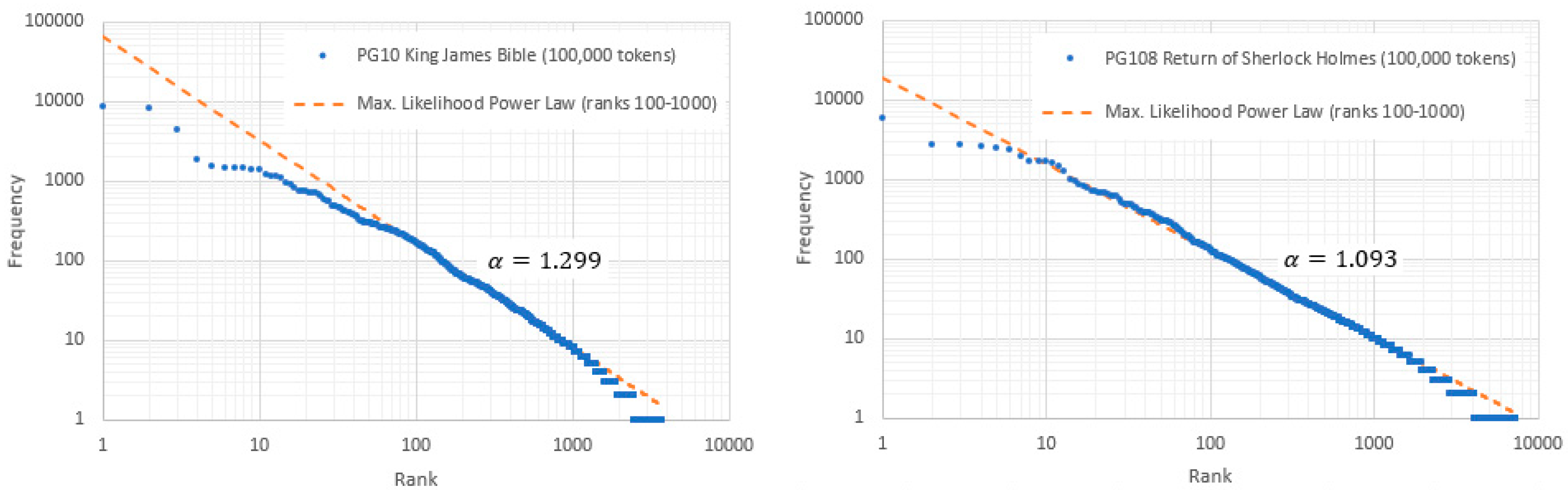
Figure 2.
Types vs. frequency plot for Corbet’s butterfly data [19] and the King James Bible (data collected by the authors), both exhibiting the Zipf size law.
Figure 2.
Types vs. frequency plot for Corbet’s butterfly data [19] and the King James Bible (data collected by the authors), both exhibiting the Zipf size law.

Figure 3.
Heaps vocabulary plots for typical English and Finnish texts, with best fit power laws overlaid.
Figure 3.
Heaps vocabulary plots for typical English and Finnish texts, with best fit power laws overlaid.

Figure 4.
Typical types vs. frequency distribution (PG10: King James Bible, first 100,000 tokens) with frequency ranges overlaid. The Zipf indices across these ranges were computed using the maximum likelihood estimation (MLE) for all 9,312 selected corpus items.
Figure 4.
Typical types vs. frequency distribution (PG10: King James Bible, first 100,000 tokens) with frequency ranges overlaid. The Zipf indices across these ranges were computed using the maximum likelihood estimation (MLE) for all 9,312 selected corpus items.

Figure 5.
Cumulative distributions of the neighbour support, for all items, using four different values of . The most extreme outliers are trimmed from the left, as (even on a logarithmic scale) their inclusion would have intolerably compressed the right-hand portion of the distribution.
Figure 5.
Cumulative distributions of the neighbour support, for all items, using four different values of . The most extreme outliers are trimmed from the left, as (even on a logarithmic scale) their inclusion would have intolerably compressed the right-hand portion of the distribution.
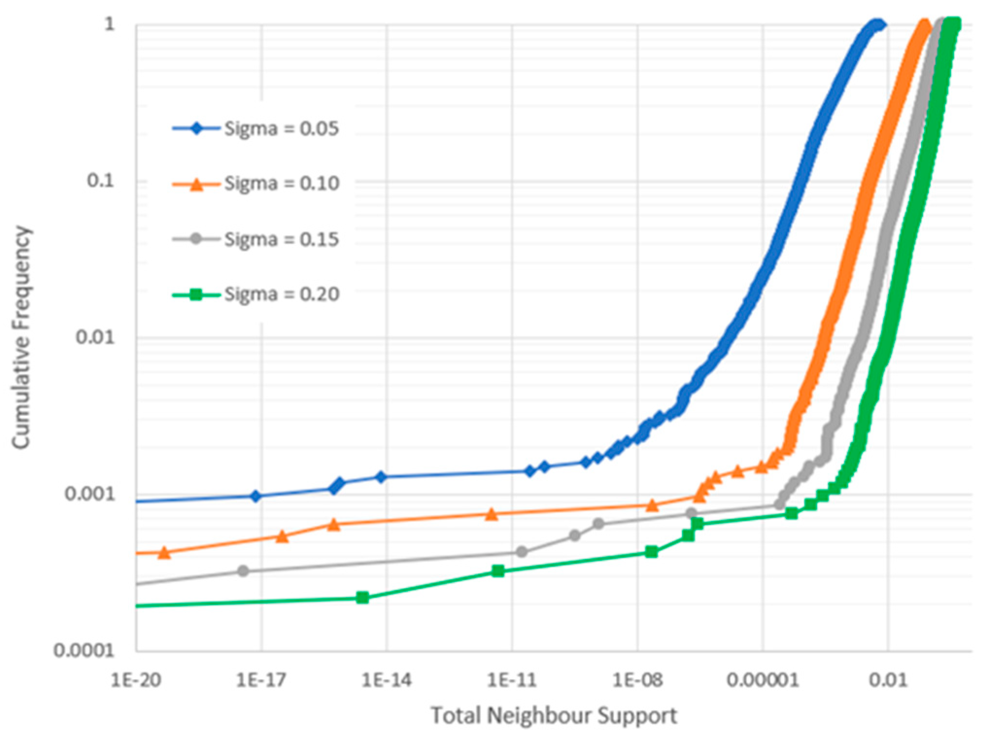
Figure 6.
Example scatter plots of obtained using different frequency ranges for items classified as anomalies and non-anomalies. The algorithm rejects egregious anomalies while accepting most plausible outliers. (a) Low and medium frequency ranges show a strong positive correlation, while (b) low and high frequency ranges exhibit a weak negative correlation (see also Table 2).
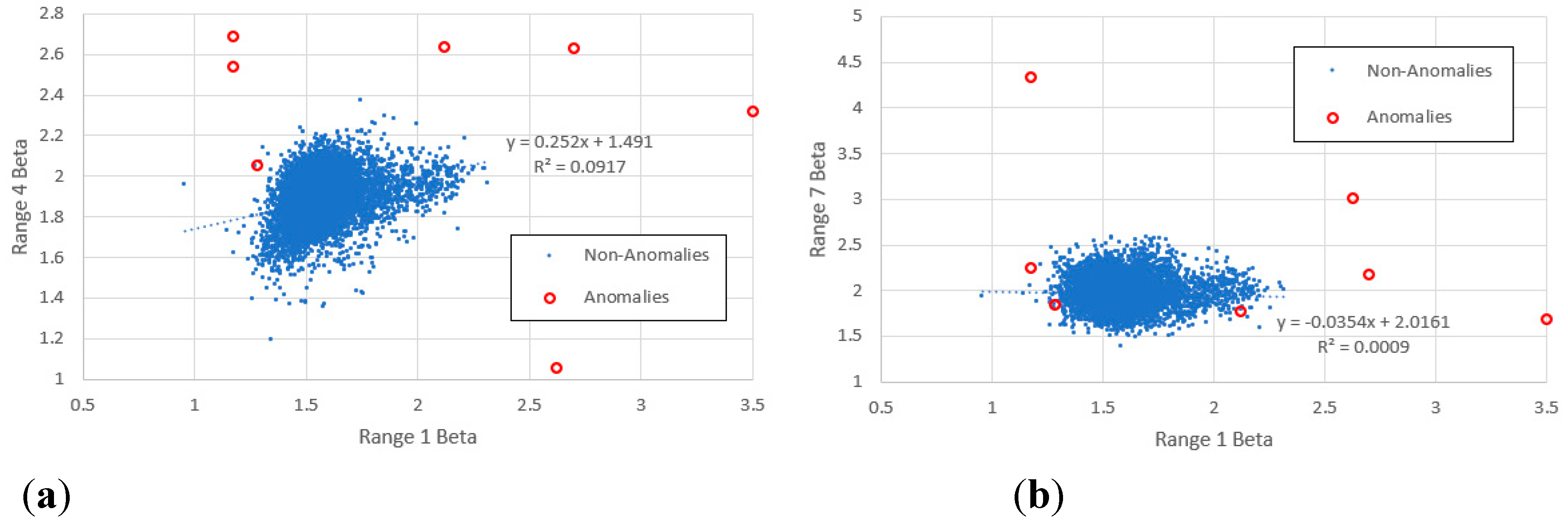
Figure 7.
(a) Median and upper and lower quartile Zipf indices computed for all seven frequency ranges and for the complete range 1-640. (b) KS significance information for the values, showing the mean and the upper and lower quartiles. The values for the frequency range 1-640 are too small to be shown meaningfully on the graph and are quoted a text box.
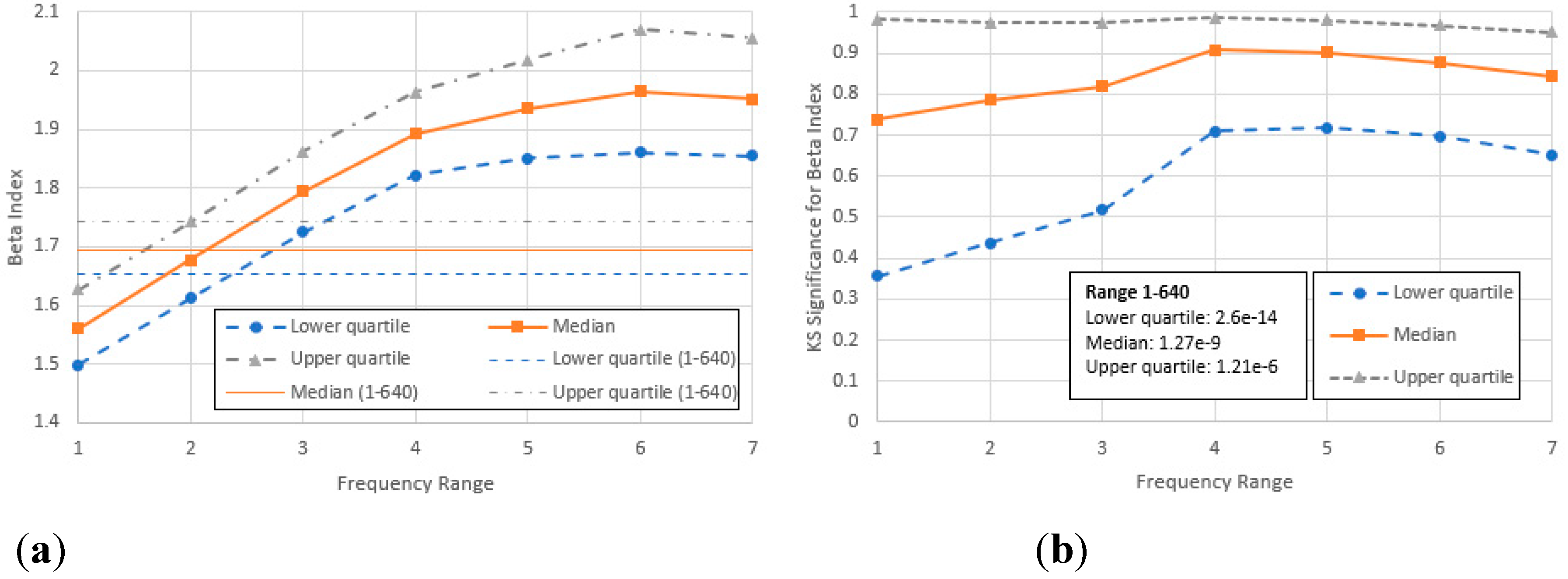
Figure 8.
Part of the cumulative frequency distribution of KS significance values obtained from ML power law fitting to ranks 100-1000, for 100,000 tokens for all PG items previously classified as non-anomalies. KS-significance represents the strength of the null hypothesis that the power law is true. Items whose distributions are shown in Figure 9 are highlighted. (The leftmost portion of the graph is truncated for greater clarity: the lowest KS significance recorded is for PG14, The 1990 CIA World Factbook.).
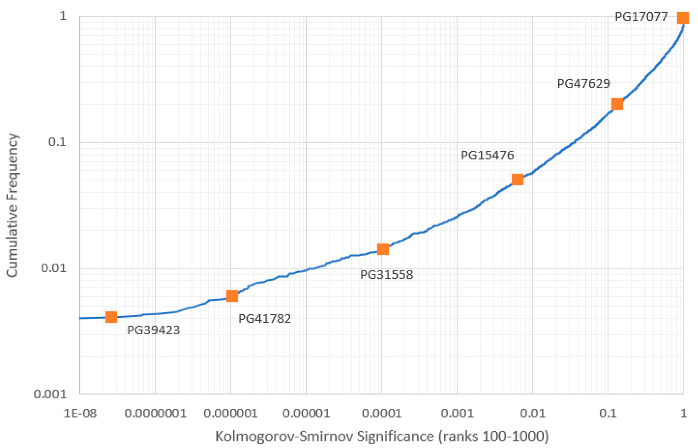
Figure 9.
Frequency/rank distributions for six PG items with different KS significances for the ML power law computed across ranks 100-1000 for 100,000 tokens. Smoothed curves were obtained using logarithmic binning. (See also Figure 8.).
Figure 9.
Frequency/rank distributions for six PG items with different KS significances for the ML power law computed across ranks 100-1000 for 100,000 tokens. Smoothed curves were obtained using logarithmic binning. (See also Figure 8.).
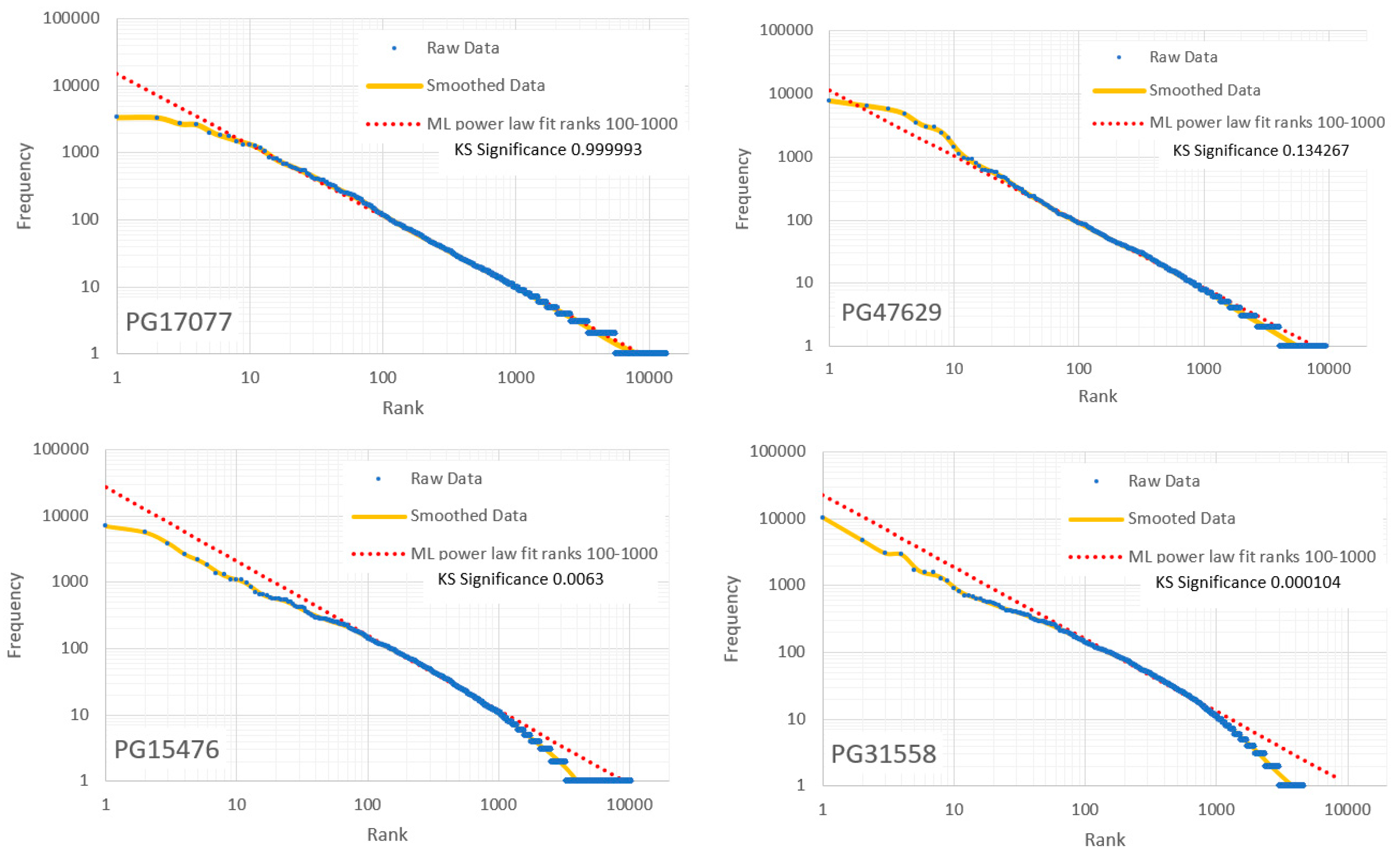
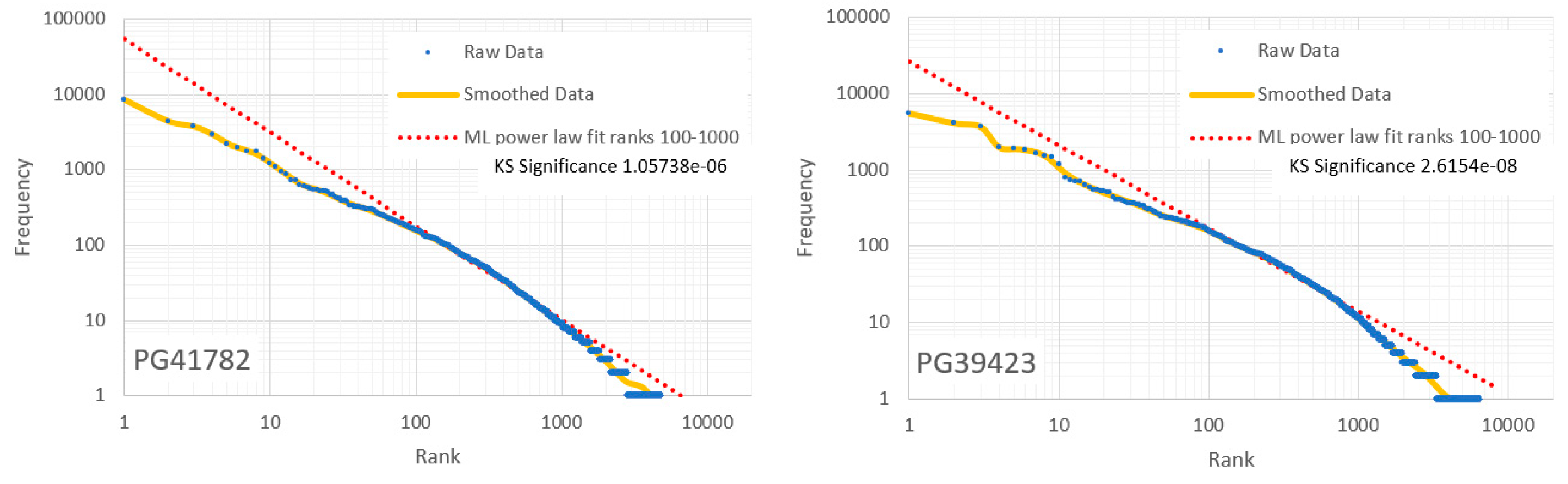
Figure 10.
Cumulative distributions of mid-range obtained for items with KS significance above and below 0.03. Note that the mean is significantly larger for the latter, but the standard deviations are almost identical.
Figure 10.
Cumulative distributions of mid-range obtained for items with KS significance above and below 0.03. Note that the mean is significantly larger for the latter, but the standard deviations are almost identical.
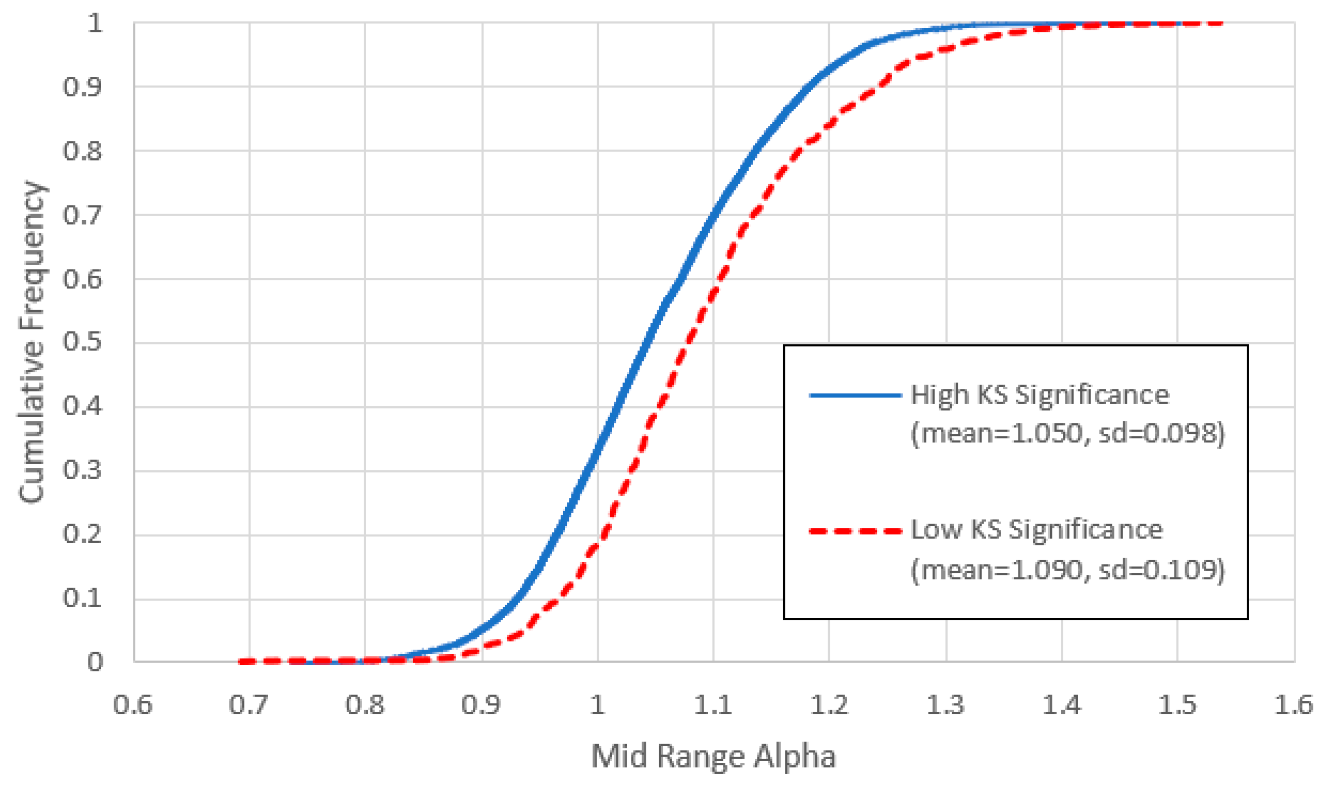
Figure 11.
(a) Non anomalous () vs. mid-range () log-log linear KS significance below and above 0.03. (b) Cumulative frequency distributions of for the lower and upper KS significances. We note the distinct cluster for the higher KS significance items (dashed rectangle, mostly Finnish items), not replicated in the lower KS items, with generally lower than those of the high KS items.
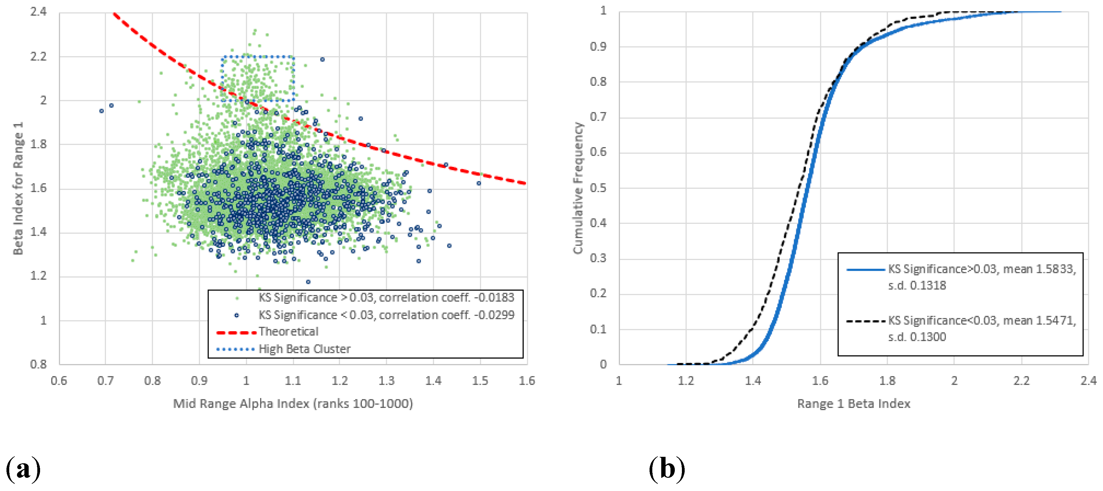
Figure 12.
(a) Non anomalous () vs. mid-range () log-log linear KS significance below and above 0.03. (b) Cumulative frequency distributions of for the lower and upper KS significances. (b) Cumulative frequency distributions of for the lower and upper KS significances. The upper cluster observed in Figure 11 has become less pronounced, though the -values for the low KS significance group are significantly lower than those of the high KS significance group and show a wider standard deviation.
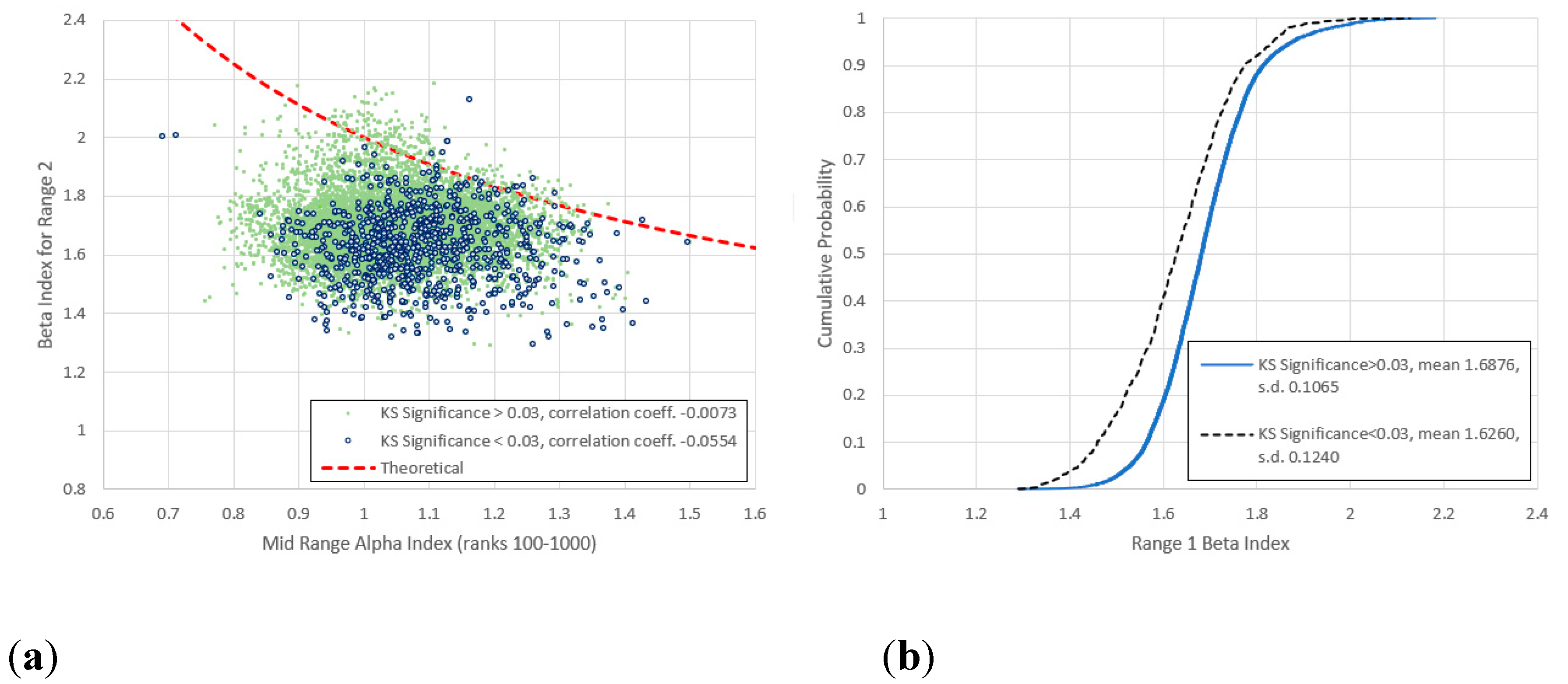
Figure 13.
(a) Comparison of mid-range and for range 3 (frequencies 4-40) for all items not previously identified as anomalies, with frequency vs. rank log-log linear KS significance below and above 0.03. (b) Cumulative frequency distributions of for the lower and upper KS significances. The upper cluster observed in Figure 11 and Figure 12 has now vanished, though the -values for the lower KS group are still significantly lower than those of the high KS significance group.
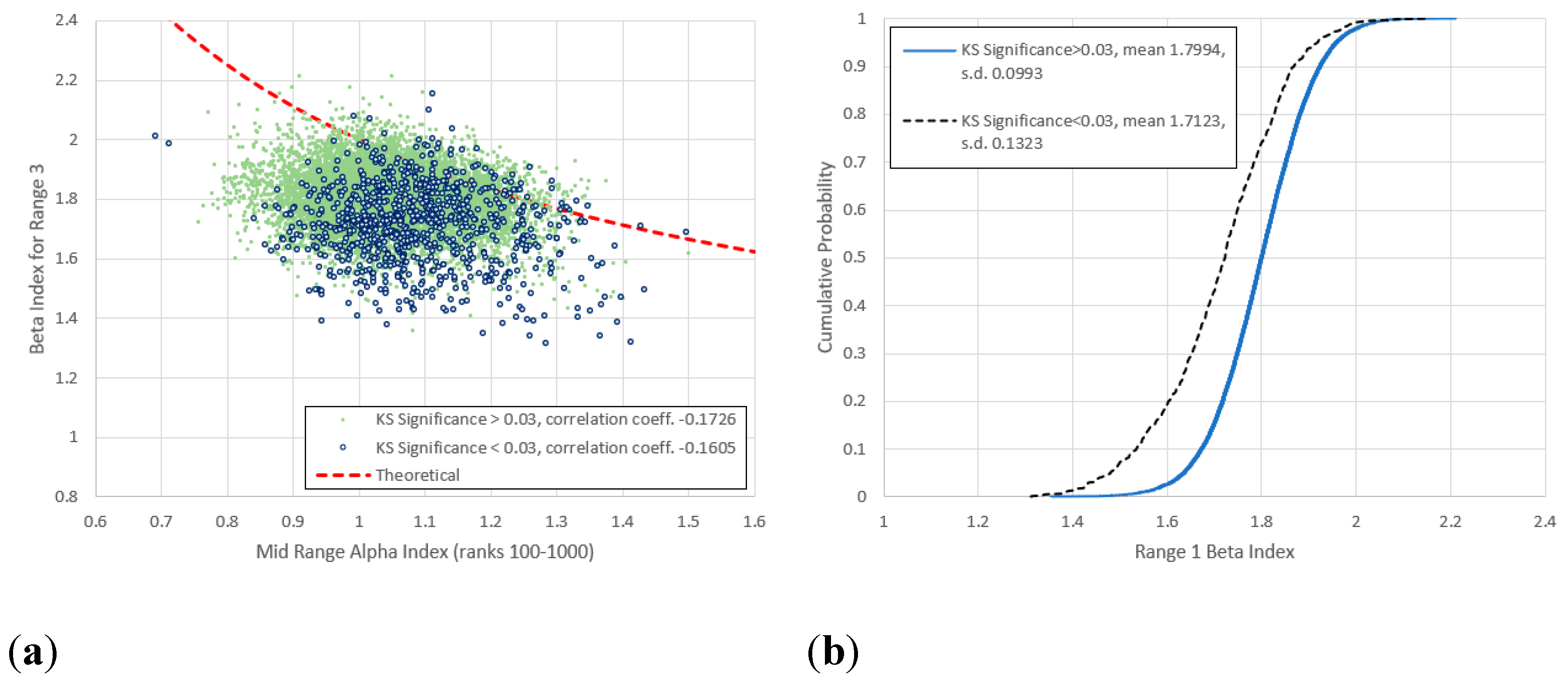
Figure 14.
(a) Comparison of mid-range and for range 4 (frequencies 8-80) for all items not previously identified as anomalies, with frequency vs. rank log-log linear KS significance below and above 0.03. (b) Cumulative frequency distributions of for the lower and upper KS significances. We note a hint of bifurcation within the low KS significance data around the theoretical line.
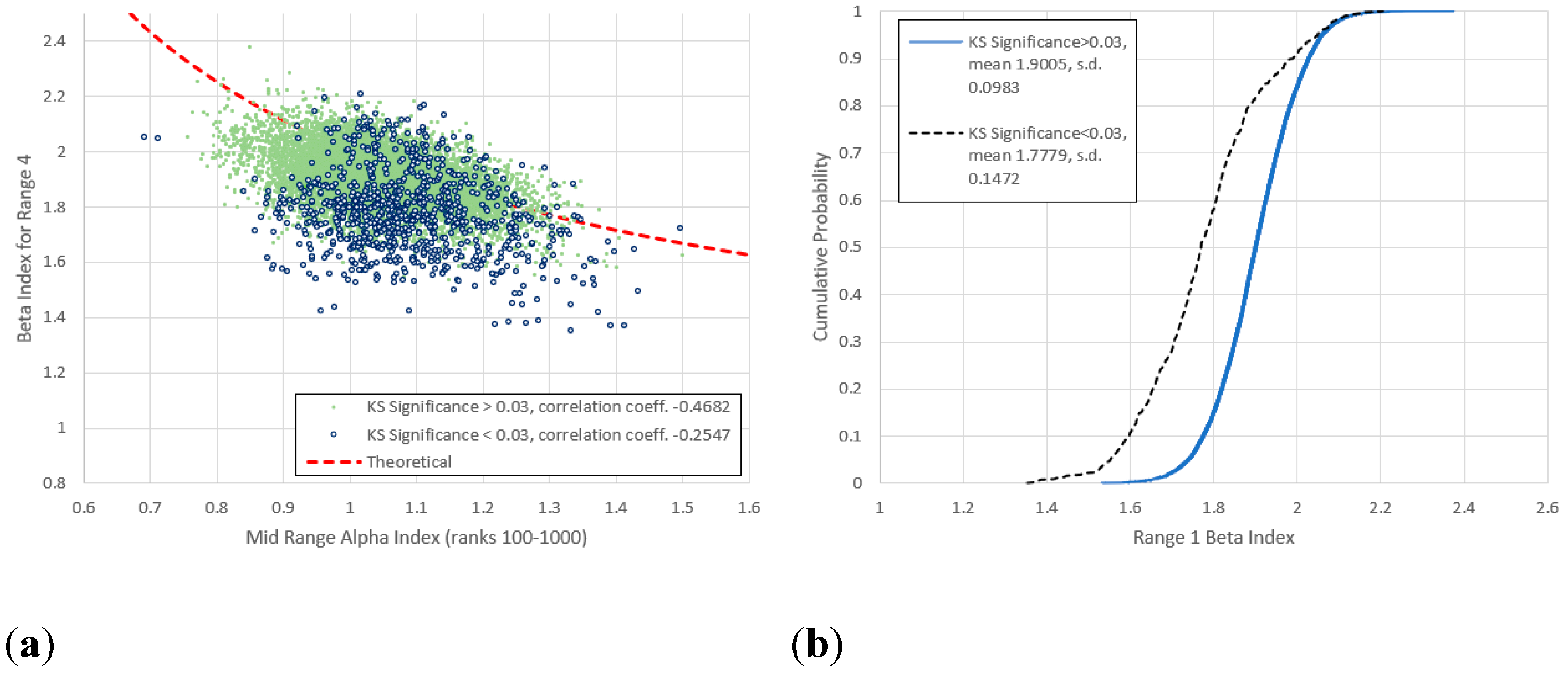
Figure 15.
(a) Comparison of mid-range and for range 5 (frequencies 16-160) for all items not previously identified as anomalies, with frequency vs. rank log-log linear KS significance below and above 0.03. (b) Cumulative frequency distributions of for the lower and upper KS significances. The bifurcation observed in Figure 15 has become much more pronounced and a low- “filament” of low KS significance items has appeared. The high KS significance items are now distributed more-or-less evenly around the theoretical curve.
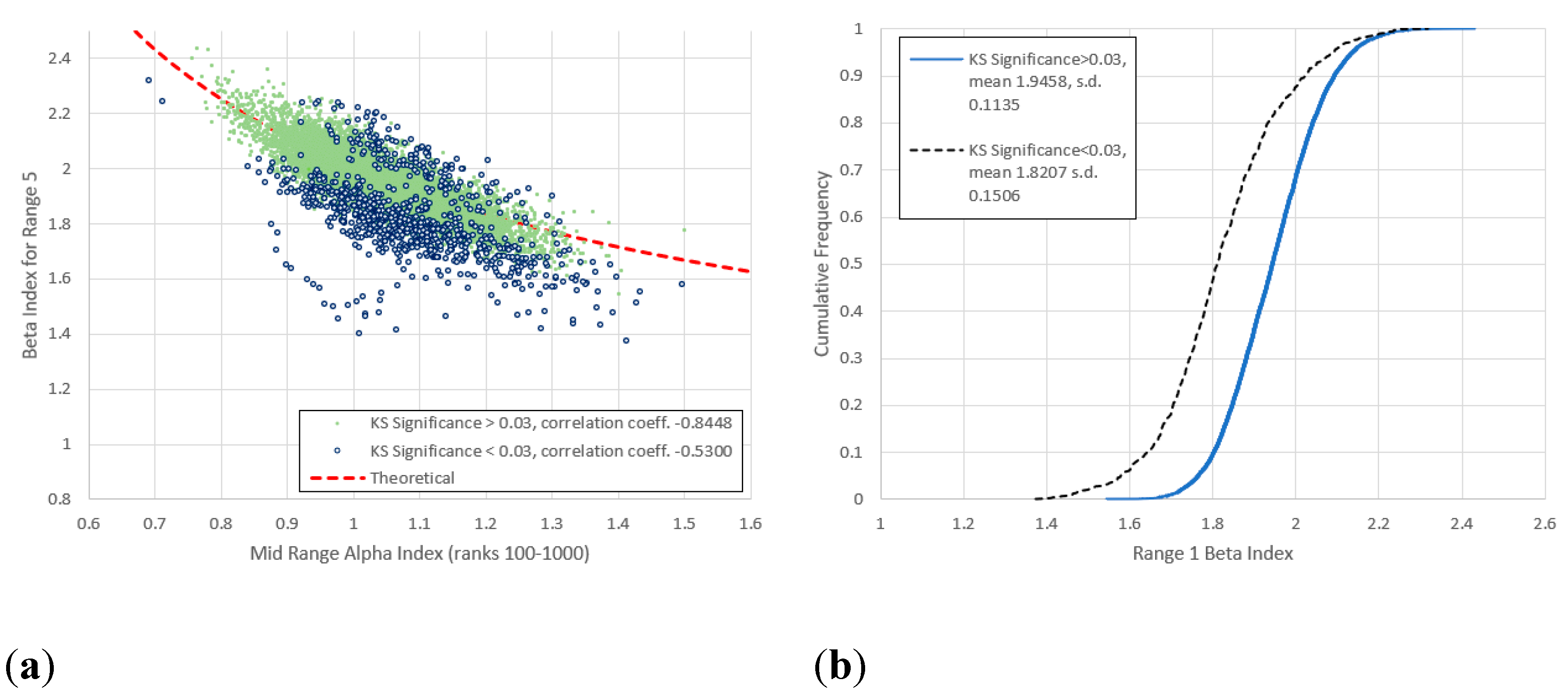
Figure 16.
(a) Comparison of mid-range and for range 6 (frequencies 32-320) for all items not previously identified as anomalies, with frequency vs. rank log-log linear KS significance below and above 0.03. (b) Cumulative frequency distributions of for the lower and upper KS significances. Bifurcation amongst the low KS significance data has now disappeared, both groups being similarly distributed. Agreement with the theoretical curve is less than in Figure 15.
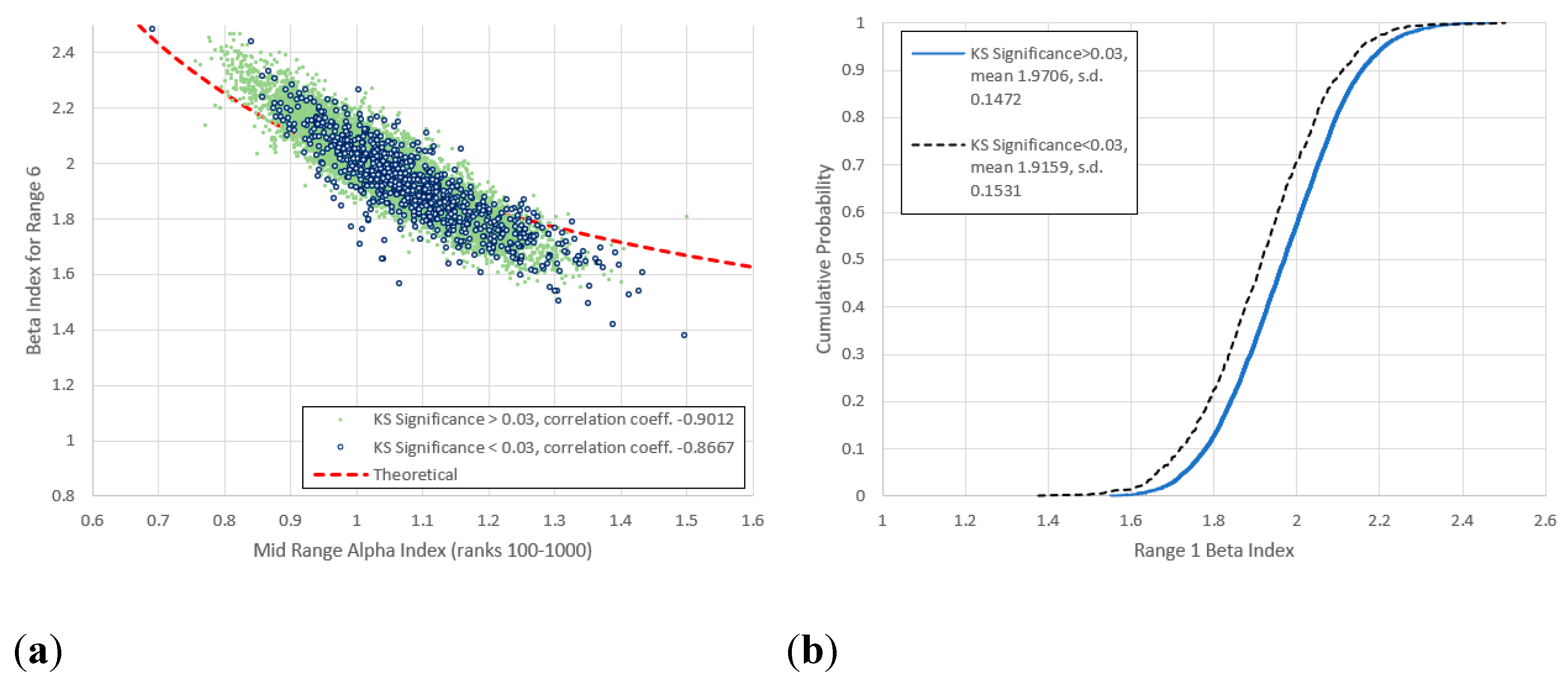
Figure 17.
(a) Comparison of mid-range and for range 7 (frequencies 64-640) for all items not previously identified as anomalies, with frequency vs. rank log-log linear KS significance below and above 0.03. (b) Cumulative frequency distributions of for the lower and upper KS significances. The high KS significance group is once again distributed evenly about the theoretical line, though the scatter is wider. Bifurcation begins to re-emerge for the low KS significance group.
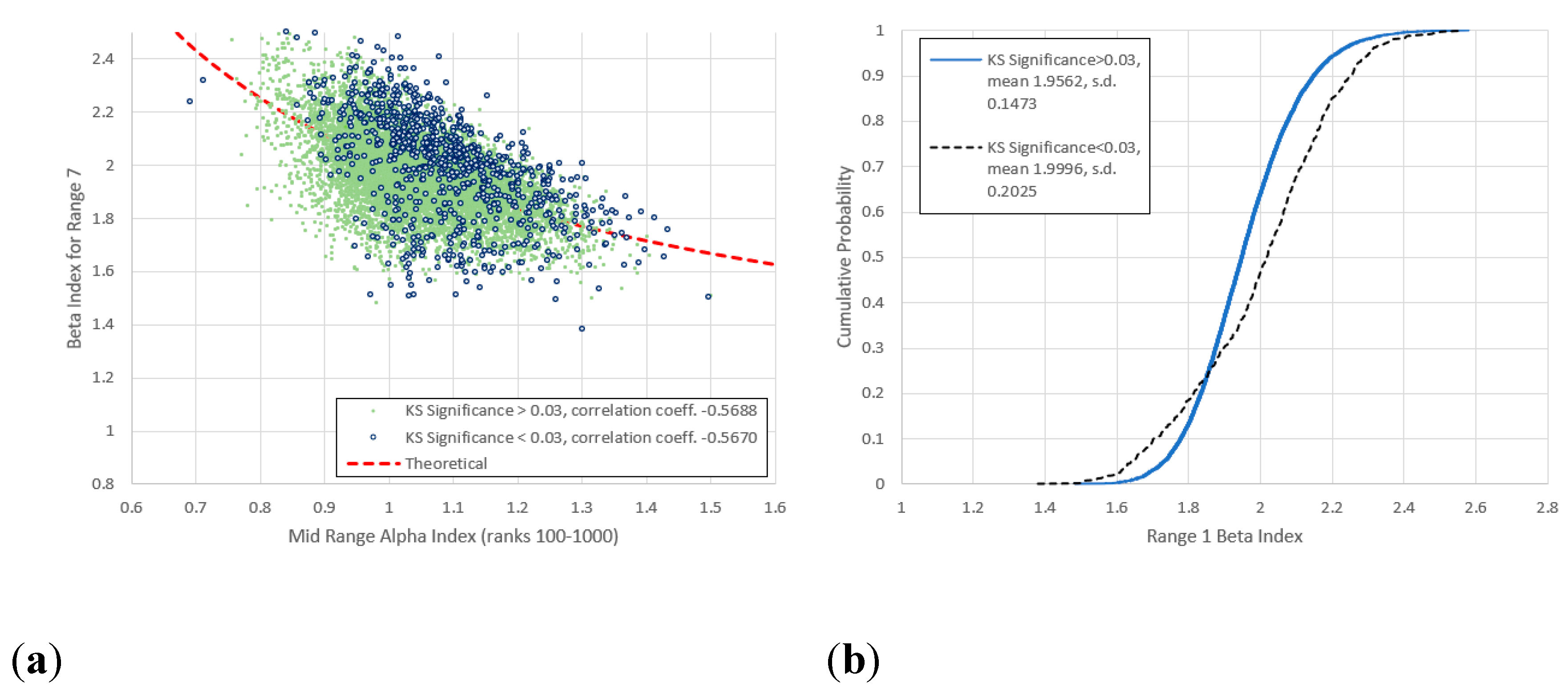
Figure 18.
Pearson correlation coefficients for vs. middle range for low and high KS-significance items across different frequency ranges. For both groups, the correlation is highest for range 6 (frequencies 32-320).
Figure 18.
Pearson correlation coefficients for vs. middle range for low and high KS-significance items across different frequency ranges. For both groups, the correlation is highest for range 6 (frequencies 32-320).
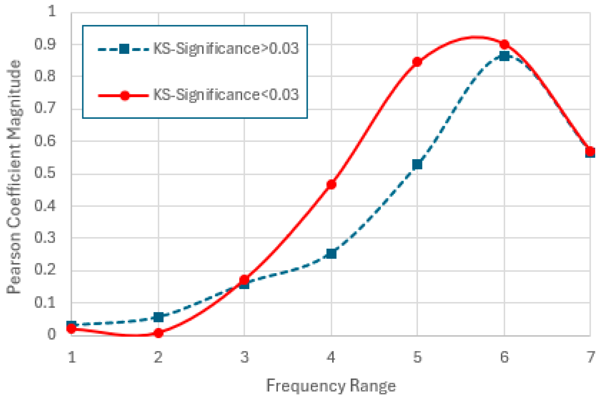
Figure 19.
Number of items in the “Finnish cluster” in range 1 (frequencies 1-10) found amongst items below a variable maximum KS-significance for mid-range . The cluster disappears amongst items with KS-significance below 0.048 beyond which it increases with the KS-significance until the latter approaches 1. The inset graph shows cluster size relative to the total number of items below the KS-significance limit, the maximum being approximately 1.55%.
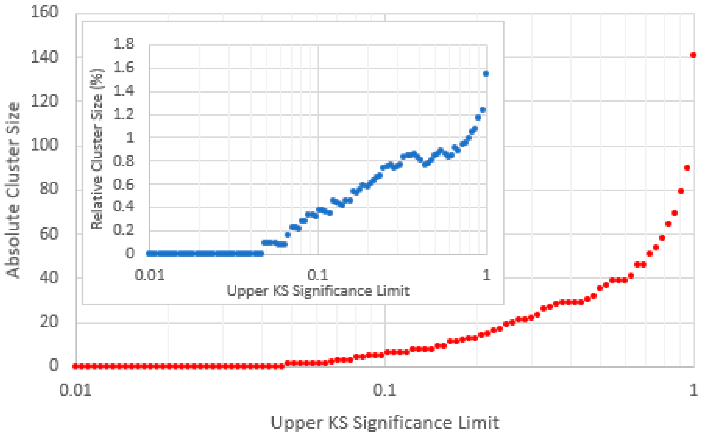
Figure 20.
Comparison of mid-range and for frequency range 11 to 120 (average range for rank range 100 to 1000 used in the calculations) with theoretical curve of (4). (a) All items not previously classified as anomalies, (b) items with a frequency vs. rank log-log linear KS-significance exceeding 0.03, (c) all items with KS-significance below 0.03 (below highlighted) and (d) items with KS-significance exceeding 0.99999.
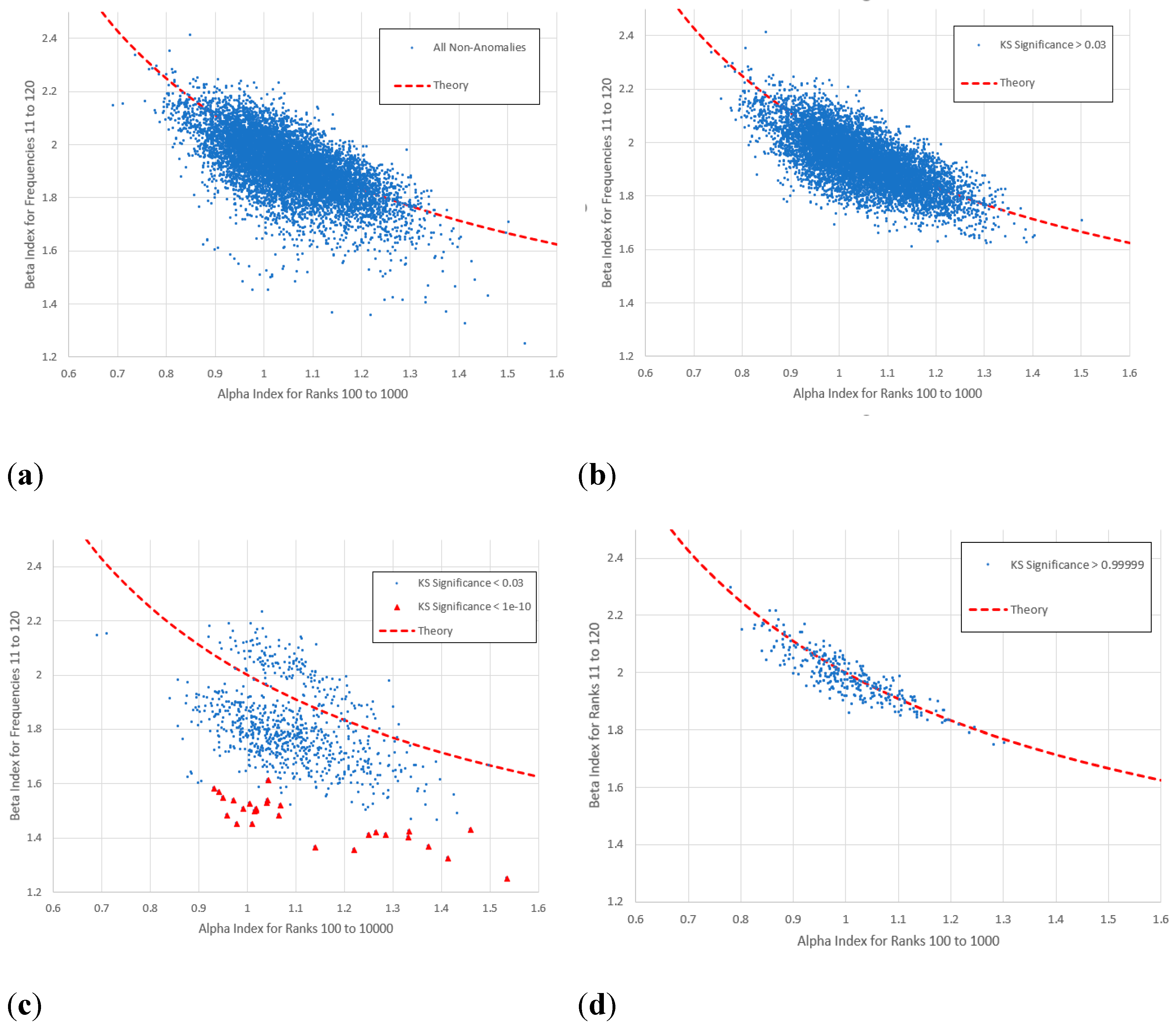
Figure 21.
Cumulative frequency distributions for optimized Heaps’ indices obtained for items with high and low KS-significance of in the middle range. We note that for the low KS-significance items, the average Heaps index is significantly lower, with a larger standard deviation.
Figure 21.
Cumulative frequency distributions for optimized Heaps’ indices obtained for items with high and low KS-significance of in the middle range. We note that for the low KS-significance items, the average Heaps index is significantly lower, with a larger standard deviation.
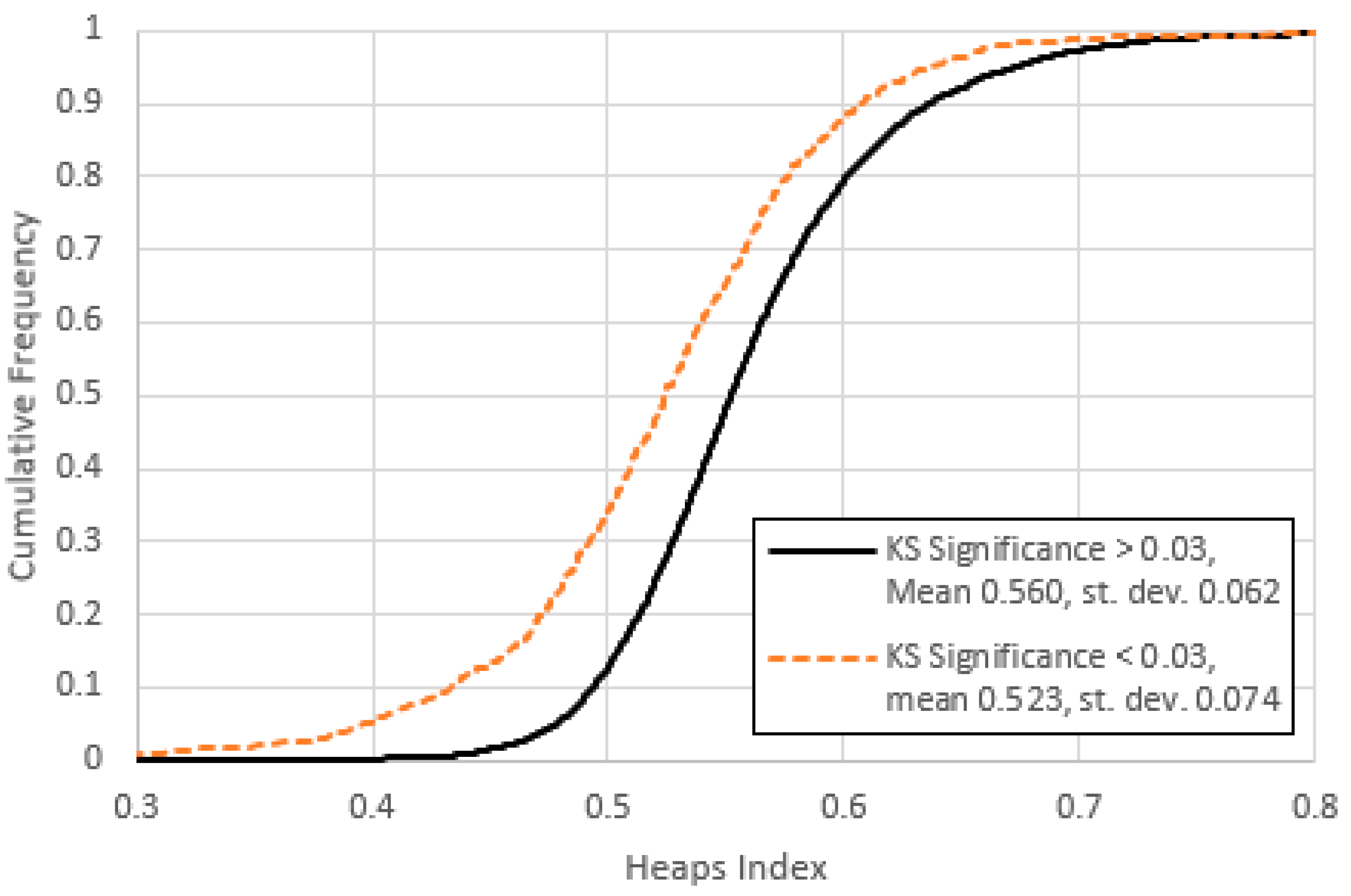
Figure 22.
Heaps index plotted against for range 1 (frequencies 1-10) for items with high and low KS-significance of in the middle range. The bulk of the data for both groups agree roughly with the theoretical line of (6). Items in the “Finnish cluster” have considerably higher than average and lie significantly above the theoretical line.
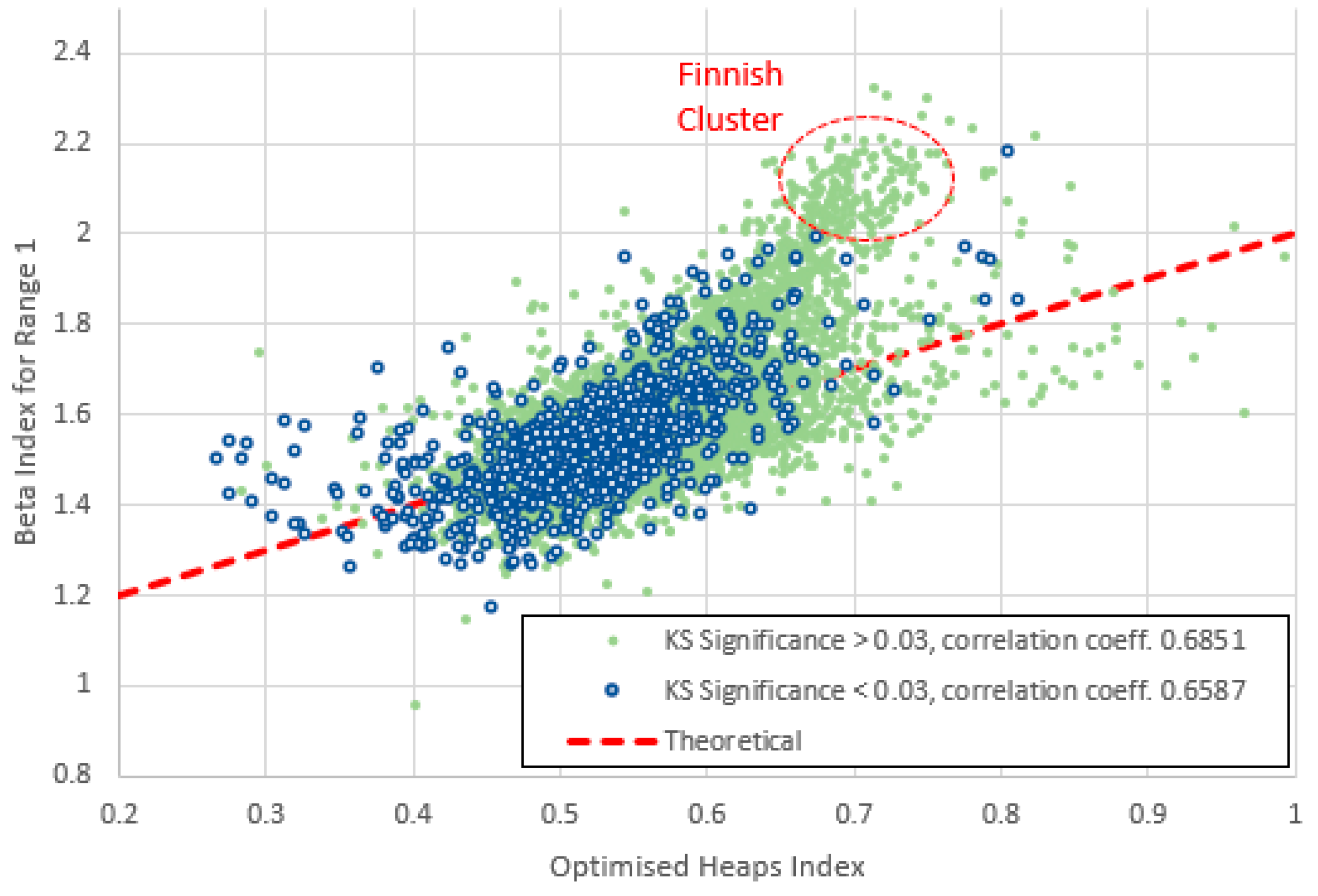
Figure 23.
Heaps index plotted against for range 2 (frequencies 2-20) for items with high and low KS-significance of in the middle range. Although the data are still strongly correlated, they now generally lie above the theoretical line of (6). The “Finnish cluster” is no longer noticeably distinct from the main body of data.
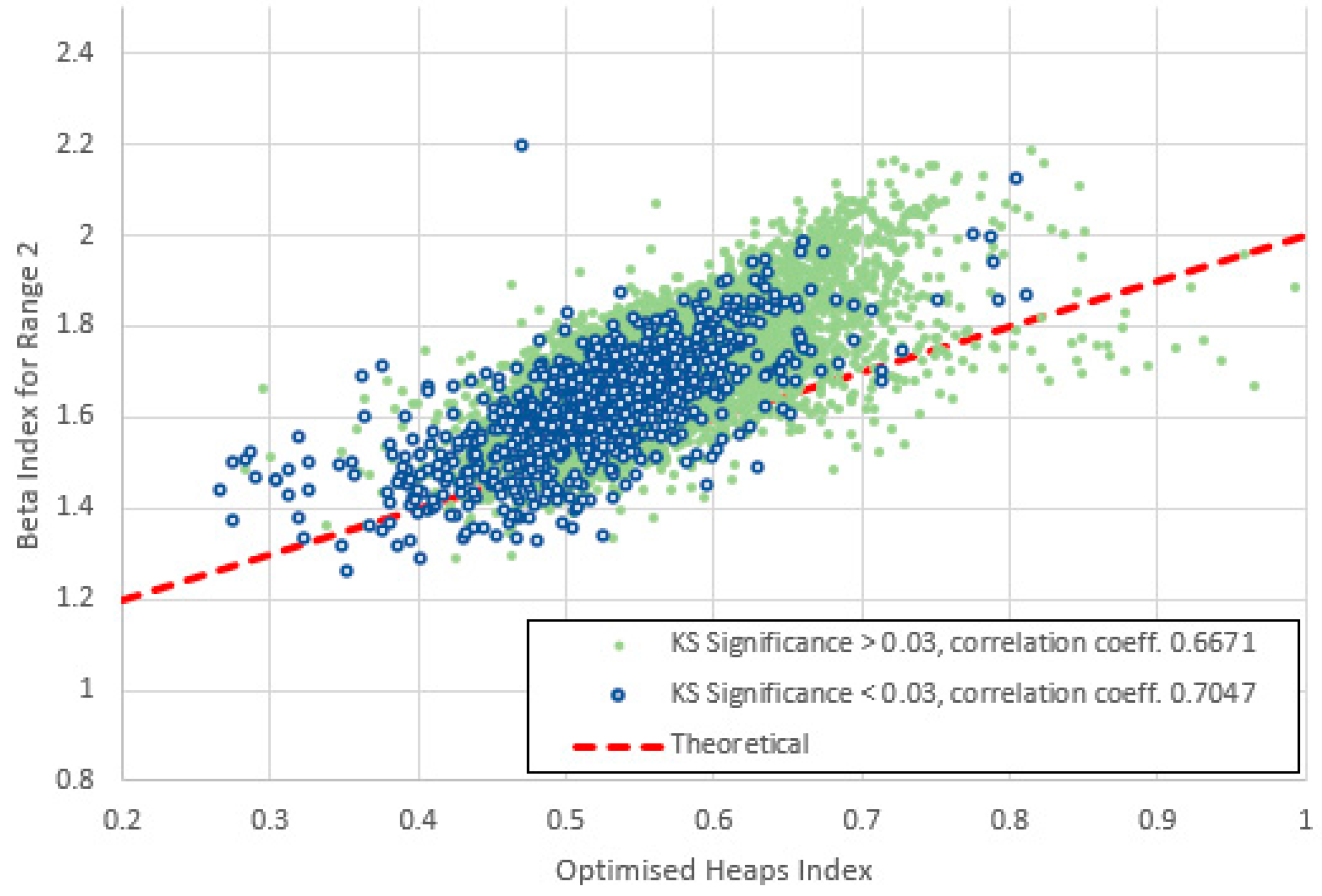
Figure 24.
Heaps index plotted against for range 3 (frequencies 4-40) for items with high and low KS-significance of in the middle range. The data are still quite strongly correlated and lie almost exclusively above the theoretical line of (6).
Figure 24.
Heaps index plotted against for range 3 (frequencies 4-40) for items with high and low KS-significance of in the middle range. The data are still quite strongly correlated and lie almost exclusively above the theoretical line of (6).
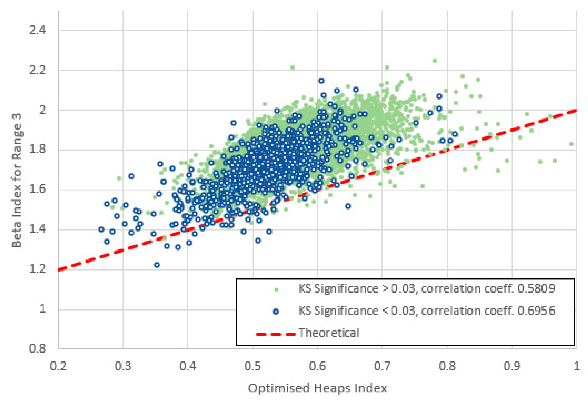
Figure 25.
Heaps index plotted against for range 4 (frequencies 8-80) for items with high and low KS-significance of in the middle range. The data are less strongly correlated than for ranges 2 and 3. The data are almost exclusively above the theoretical line of (6). Interestingly the base of each cluster lies approximately parallel with this line.
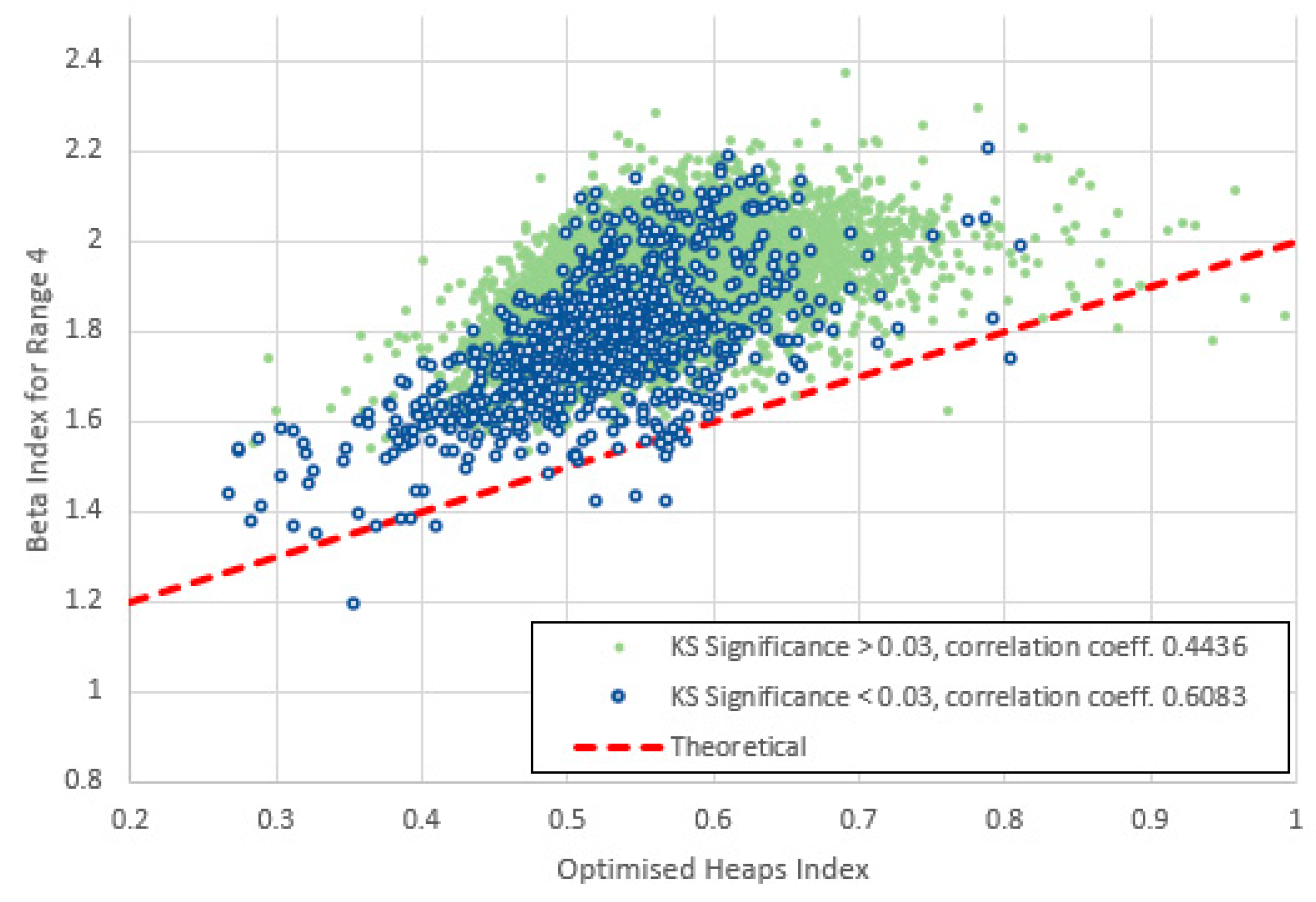
Figure 26.
Heaps index plotted against for range 5 (frequencies 16-160) for items with high and low KS-significance of α in the middle range. The data are less strongly correlated than for range 4 and lie more distinctly above the theoretical line of (6). The bases of both clusters are still roughly parallel with this line.
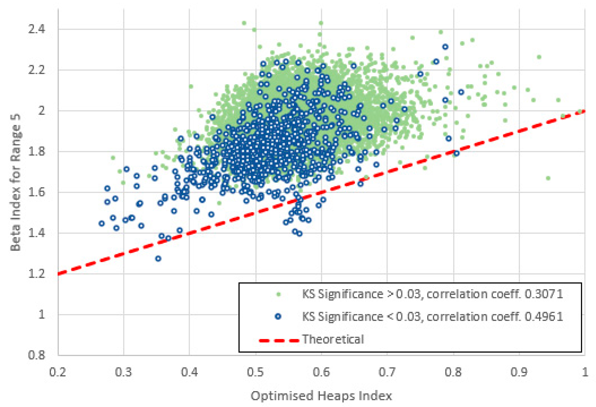
Figure 27.
Heaps index plotted against for range 6 (frequencies 32-320) for items with high and low KS-significance of in the middle range. The data are no longer strongly correlated and lie distinctly above the theoretical line of (6). The clusters no longer show clear linear bases.
Figure 27.
Heaps index plotted against for range 6 (frequencies 32-320) for items with high and low KS-significance of in the middle range. The data are no longer strongly correlated and lie distinctly above the theoretical line of (6). The clusters no longer show clear linear bases.
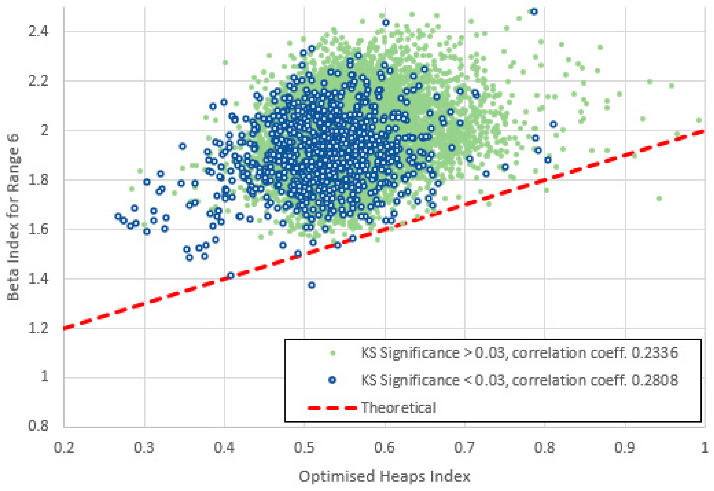
Figure 28.
Heaps index plotted against for range 7 (frequencies 32-320) for items with high and low KS-significance of in the middle range. The data are no longer strongly correlated and lie distinctly above the theoretical line of (6). The clusters no longer show clear linear bases.
Figure 28.
Heaps index plotted against for range 7 (frequencies 32-320) for items with high and low KS-significance of in the middle range. The data are no longer strongly correlated and lie distinctly above the theoretical line of (6). The clusters no longer show clear linear bases.
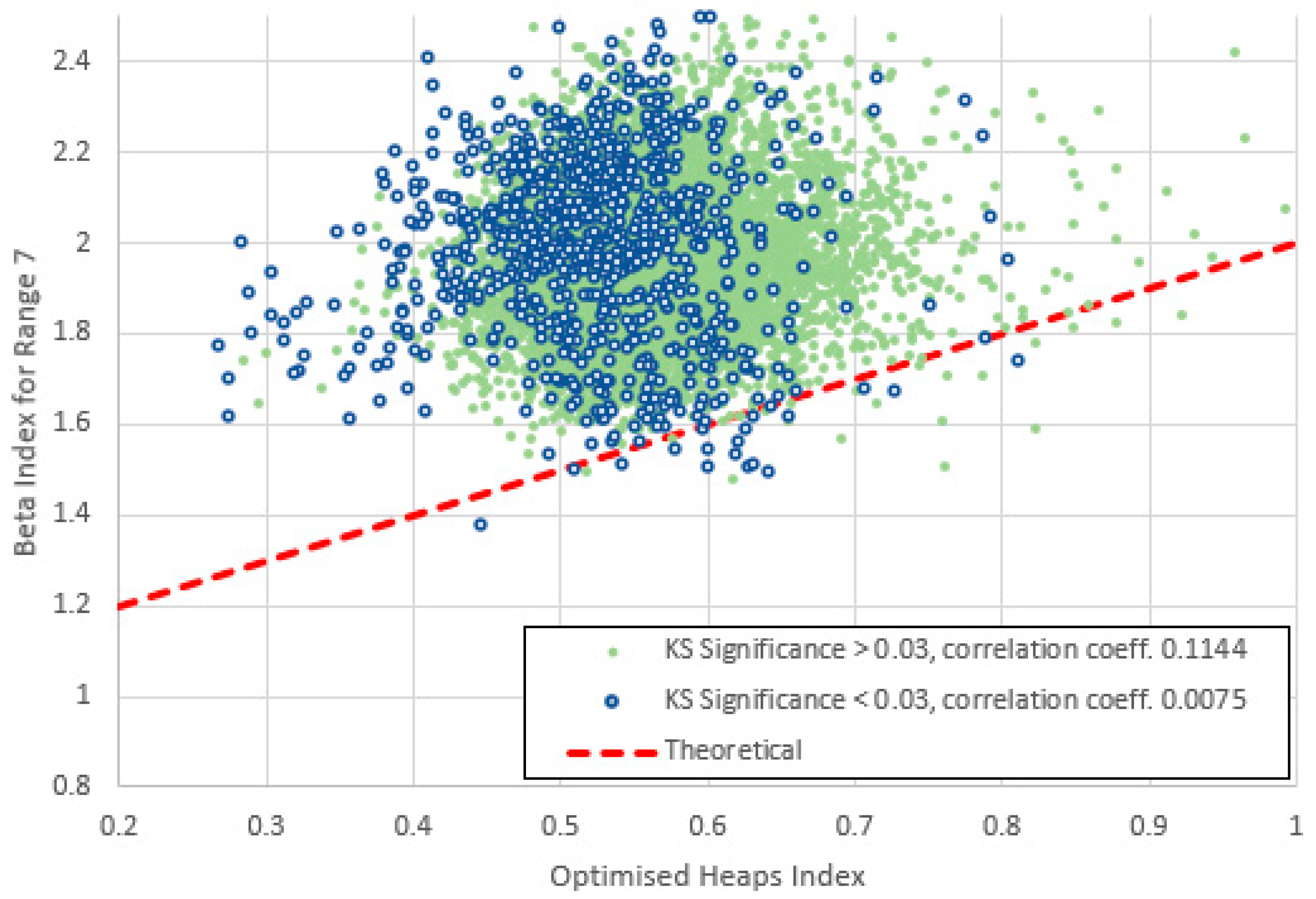
Figure 29.
Variation of Pearson correlation coefficients for vs across the seven frequency ranges for items high and low KS-significance of α in the middle range. Both groups show a high correlation for low frequencies, decreasing rapidly as frequency increases.
Figure 29.
Variation of Pearson correlation coefficients for vs across the seven frequency ranges for items high and low KS-significance of α in the middle range. Both groups show a high correlation for low frequencies, decreasing rapidly as frequency increases.
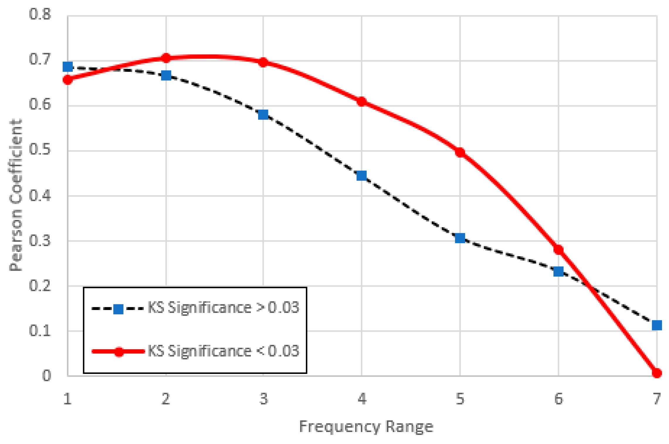
Figure 30.
Scatter plots of (a) low and (b) high-frequency indices vs. the optimised Heaps index obtained by simulation using the simplified model of (11). We note the qualitative agreement between these and the real results of Figure 22, Figure 23, Figure 24, Figure 25, Figure 26, Figure 27 and Figure 28. Results are based on 500 independent simulations.
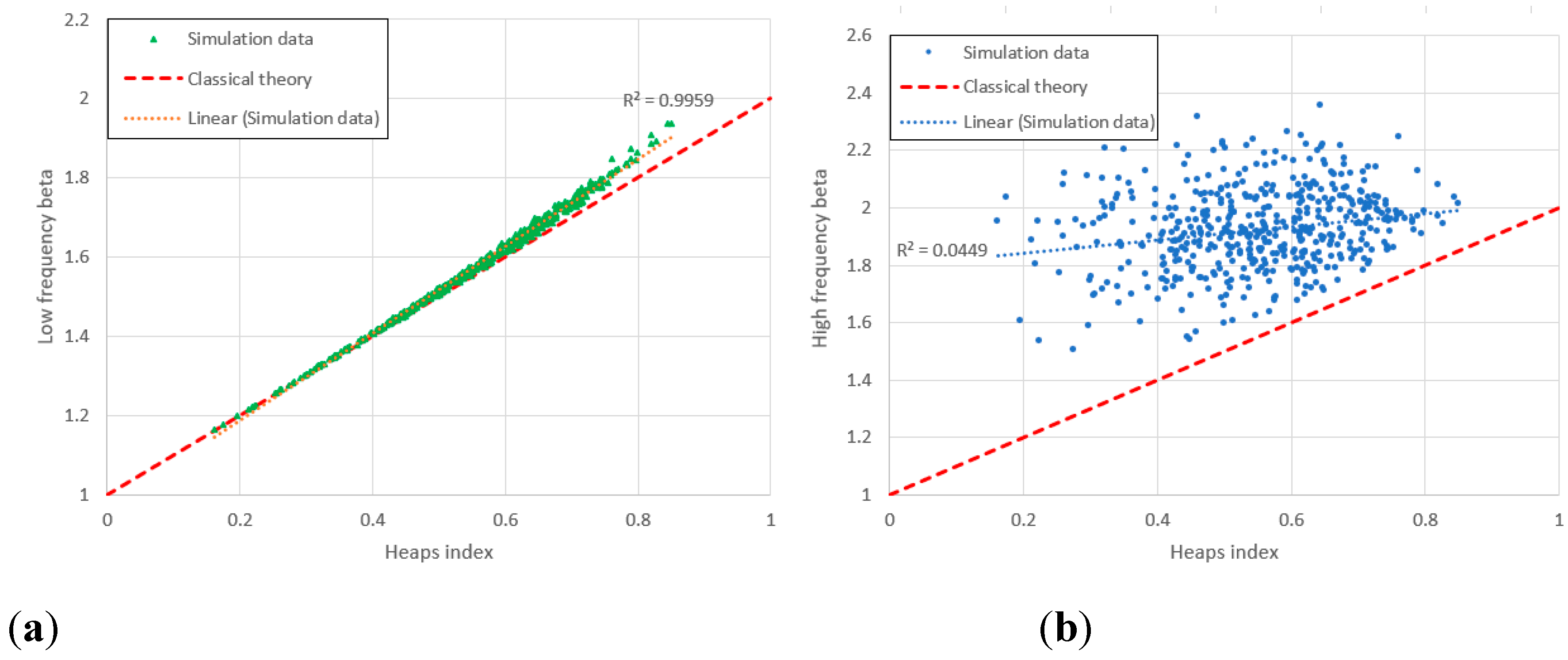

Table 1.
The seven lowest scoring items by support (anomalies) together with the seven highest scoring items. EDNN is “Euclidean distance to the nearest neighbour” in 7-dimensional -space. Anomalies are mostly dictionaries while top scoring items include many theological works.
Table 1.
The seven lowest scoring items by support (anomalies) together with the seven highest scoring items. EDNN is “Euclidean distance to the nearest neighbour” in 7-dimensional -space. Anomalies are mostly dictionaries while top scoring items include many theological works.
| Code | Title (abbreviated) | Author | ) | EDNN |
|---|---|---|---|---|
| PG51155 | Dictionary of Synonyms and Antonyms | Samuel Fallows | 2.40E-82 | 2.837 |
| PG22722 | Glossary for Spelling of Dutch Language | Matthais de Vries | 1.36E-23 | 1.400 |
| PG10681 | Thesaurus of English Words and Phrases | Peter Mark Roget | 3.73E-18 | 1.190 |
| PG19704 | A Pocket Dictionary: Welsh-English | William Richards | 1.71E-11 | 0.841 |
| PG38390 | A Dictionary of English Synonyms | Richard Soule | 3.38E-10 | 0.760 |
| PG20738 | English-Spanish-Tagalog Dictionary | Sofronio Calderón | 1.18E-09 | 0.721 |
| PG19072 | Selected Pamphlets of the Netherlands | - | 1.93E-07 | 0.594 |
| PG23637 | The Bishop of Cottontown | John Moore | 0.222025 | 0.0565 |
| PG36909 | Memoirs of General Baron de Marbot (v.1) | Baron de Marbot | 0.222453 | 0.0410 |
| PG42645 | Expositor's Bible: Galatians | George Findlay | 0.223936 | 0.0452 |
| PG8069 | Expositions of Scripture: Isaiah & Jeremiah | Alexander Maclaren | 0.224487 | 0.0410 |
| PG3434 | Social Work of the Salvation Army | Henry Rider | 0.224566 | 0.0023 |
| PG2800 | The Koran | - | 0.224596 | 0.0023 |
| PG45143 | The Way to the West – 3 Early Americans | Emerson Hough | 0.224600 | 0.0312 |
Table 2.
Pearson correlation coefficients computed between -values for all non-anomalies for frequency ranges (See Figure 3). Generally, the closer two ranges are, the more positive the correlation; widely different ranges have weak (though significantly) negative correlation. (Green and yellow highlights indicate for positive and negative correlation respectively.).
 |
Disclaimer/Publisher’s Note: The statements, opinions and data contained in all publications are solely those of the individual author(s) and contributor(s) and not of MDPI and/or the editor(s). MDPI and/or the editor(s) disclaim responsibility for any injury to people or property resulting from any ideas, methods, instructions or products referred to in the content. |
© 2025 by the authors. Licensee MDPI, Basel, Switzerland. This article is an open access article distributed under the terms and conditions of the Creative Commons Attribution (CC BY) license (http://creativecommons.org/licenses/by/4.0/).
Copyright: This open access article is published under a Creative Commons CC BY 4.0 license, which permit the free download, distribution, and reuse, provided that the author and preprint are cited in any reuse.


