
Submitted:
01 April 2025
Posted:
03 April 2025
You are already at the latest version
Abstract
Microplastics (MPs) have emerged as a major pollutant in aquatic ecosystems, primarily originating from industrial activities and plastic waste degradation. Understanding their transport dynamics is crucial for assessing environmental risks and developing mitigation strategies. This study employs Computational Fluid Dynamics (CFD) simulations to model the trajectory of MPs in section B of the Salado Estuary in the city of Guayaquil, Ecuador, using ANSYS FLUENT 2024 R2. The transient behavior of Polyethylene Terephthalate (PET) particles was analyzed using the Volume of Fluid (VOF) multiphase model, k-omega SST turbulence model, and Discrete Phase Model (DPM) under a continuous flow regime. Spherical PET particles (5 mm diameter, 1340 kg/m³ density) were introduced at water velocities of 0.5 m/s and 1.25 m/s. Density contour analysis facilitated the modeling of the air-water interface, while particle trajectory analysis revealed that at 0.5 m/s, particles traveled 18–22.5 meters before sedimentation, whereas at 1.25 m/s, they traveled 50–60 meters before reaching the bottom. These findings demonstrate that higher flow velocities enhance MP transport distances before deposition, emphasizing the role of hydrodynamics in microplastic dispersion. This study underscores the potential of CFD as a predictive tool for assessing MP behavior in aquatic environments, contributing to improved pollution control and remediation efforts.
Keywords:
microplastics
; computational fluid dynamics
; water bodies
; PET
; discrete phase model
; open channel flow
1. Introduction
Microplastics (MPs) are particles with a diameter of less than 5 mm [1]. Marine ecosystems are particularly vulnerable to pollution due to various human and industrial activities, such as the dumping of plastic waste into oceans, seas, and rivers [2],[3] Over time, exposure to the sun's rays causes these plastics to fragment into smaller particles, called MPs [4]
MPs can be classified into two types according to their origin: primary and secondary [5]. Primary MPs are deliberately manufactured for specific uses, such as microspheres and granules [6], [7]. These microplastics are incorporated into consumer products such as cosmetics, cleaning products, paints, and scrubs, as they replace natural ingredients, which are often more expensive [8]. In addition, pellets are used in the manufacture of larger plastics, used in processes such as molding and extrusion, to create plastic objects from melting them into specific molds [9].
Secondary MPs, on the other hand, are the result of the breakdown of larger plastics, which fragment into small particles due to exposure to environmental factors [10], [11]. In some cases, they can also be generated through biological processes, as certain plastics can biodegrade by the action of bacteria and fungi [12]. The main sources of secondary MPs include common plastic waste such as bottles, bags, and packaging [13]. In less developed countries, natural disasters, such as tsunamis, hurricanes, and high tides, also contribute to pollution, as large amounts of waste can reach the sea [14].
The plastics most commonly found in MPs include materials such as polyethylene terephthalate (PET), polyester (PES), low-density polyethylene (LDPE), high-density polyethylene (HDPE), polyvinyl chloride (PVC), polypropylene (PP), polyamide (PA), polystyrene (PS), acrylonitrile-butadiene-styrene (ABS), and polytetrafluoroethylene (PTFE) [15].
PET is a thermoplastic polyester that has two characteristics [16] it acts as an amorphous plastic when cooled rapidly, however, when it behaves as a semi-crystalline plastic it cools slowly [17]. It is classified as one of the most widely used plastic materials in the industry due to its excellent physical and chemical properties. It has a transparent color and is used in the manufacture of bottles, food packaging, or in the textile industry as a synthetic fiber [18], [19].
In a previous investigation, several types of MPs were detected in a water distribution network, but PET was among the most common with a concentration of 0.0189 microplastics per liter (MPs/L) [20]. Analyses of different consumer products reveal the wide distribution of PET. First, PET was detected in drinking water processed in Germany along with other polymers, with concentrations of these particles ranging from 0.001 to 0.197 particles per litre [21], this highlights the contamination of drinking water, derived from filtered systems or pipes. Secondly, in plastic bottles of mineral water in Germany, higher concentrations of PET were found, with values ranging from 2649 ± 2857 particles per liter [22] suggesting that prolonged contact of the liquid with the container favors the release of microplastics. Finally, in the beers analyzed in Mexico, PET particles were identified in sizes from 100 to 3000 μm with a concentration of 152 ± 50.97 particles per liter [23].
Kabir et al. (2025) applied CFD, using the VOF coupled with the DPM model, for tracking the spatial distribution of MPs and showing that the size of the particles and their density are determinant in their mobility. The project was carried out in a wetland environment subjected to stormwater conditions, through which it was analyzed how various variables of MPs influence the movement and dispersion of particles. The simulations were carried out in 200 seconds, using two velocities for water 0.1 m/s and 0.3 m/s, and constant air velocity 2.5 m/s. The simulations showed that particles of greater size and density in spherical shape tended to concentrate near the inlet zone when the water velocity was low, due to their limited mobility and rapid sedimentation. In contrast, smaller particles, having less inertia, remained in suspension longer and were transported farther [24].
According to the study by Ioakeimidis et al. (2016) the progressive degradation of PET in marine environments begins approximately after 15 years of exposure. Through ATR-FTIR spectrometry characterization, they identified structural changes in the recovered bottles, including the loss of native functional groups and the appearance of new compounds, indicating chemical modifications induced by environmental factors. This study was conducted in the Ionian Sea and the Saronic Gulf, providing crucial information on the longevity of PET [25]
Fatahi et al. (2021), performed numerical simulations to study the effects of different variables on the distribution of MPs in a coastal marine environment. VOF wave models and First Airy wave model coupled with DPM were used. In their work, they dumped particles of PET (Polyethylene Terephthalate), PU (Polyurethane) and PP (Polypropylenes) from the coast to carry out the investigation of the type, size and shape of the MPs with two ocean water flow rates and different temperature conditions [26].
Quyen and Choi (2022), implemented a two-dimensional numerical wave channel that simulates intermediate waves with a weak current in a coastal area to investigate the behaviors of MPs corresponding to parameters such as particle size (0.2, 1 and 5 mm), particle density (900, 1000 y 1100 ), and a submerged artificial structure [27]
Then, Quyen et al. (2024) used CFD to analyze how different types of breakers influence the dispersion and accumulation of MPs in a coastal area. The importance of the interaction between inertia and viscosity in the advection of particles was highlighted, showing that particles of MPs with smaller size can move more easily due to an optimal balance between forces. The research emphasizes the potential for future studies in three-dimensional environments and with more complex shapes of MPs, which will allow a more complete analysis of their behavior in the ocean [28]
In another study, Dichgan et al. (2023), used numerical modeling to investigate the transport and retention of MPs in a hyporheic zone. The simulations performed for the transfer and infiltration of 1 μm MP particles in a sandy river bed showed that the advection-diffusion equation can be used to appropriately represent the transport of MP particles of pore scale size within the hyporheic zone. To corroborate the applicability of the numerical model, they repeated the experiment with 10 μm particles and were able to determine that these MPs particles manifest delayed infiltration and transport behavior. The numerical model was able to effectively represent the transport and retention of MPs in the hyporheic zone [29].
In their study, Ding et al. (2019), "Numerical Prediction of the Short-Term Path of PM Particles in Laizhou Bay" analyzes the pathways of PM particles released from four river mouths adjacent to Laizhou Bay employing the Boltzmann network method in conjunction with the Lagrange particle tracking method, which involves particle collisions and particle-wall collisions. The paths of particles emitted from four river mouths were documented over a period of thirty days [30]
In his research, Molazadeh et al. (2023), analyze the accumulation of MPs in the sediments of a stormwater pond and examine 13 sediment samples for MPs with a size of up to 10 μm, with an average abundance of number and mass of MPs of 11.8 μg/kg and 44,383 items/kg, respectively. These particles were unevenly distributed, with conditions varying two orders of magnitude within the pond. Floating MPs accounted for 95.4% of the total mass and 83.5% of the total number, with polypropylene predominating, followed by polyethylene. They created a CFD model that was used to simulate transport mechanisms that run from water to sediment. Advection and dispersion turned out to be the main mechanisms of transport of MPs to sediments, suggesting that a fraction of these particles were trapped in the bed, reducing their impact on water bodies [31].
Therefore, this study focuses on a segment of Section B of the Salado Stuary, located in the city of Guayaquil. This area was selected due to its high level of contamination, evidenced by the accumulation of solid waste in its mangroves, including plastic bags, PET bottles, disposable cups, and other polluting materials [5]. It has been proposed to simulate the trajectory of MPs in this sector using the ANSYS FLUENT 2024 R2 software.
For the simulation, data were collected that allowed the initial parameters to be established. Subsequently, the appropriate models to address the problem were defined, based on literature reviews that support the use of CFD as an effective tool to analyze the trajectory and dispersion of MPs in water bodies [26]
The Salado Estuary of Guayaquil is an ecosystem where pollution by MPs is evident, mainly due to the accumulation of plastic waste. "Pollution is one of the main evils that afflict the estuaries of Guayaquil, and every day in the branches of the Salado estuary, tubs, garbage bags and plastic bottles accumulate."[32] The constant presence of this waste favors the generation of MPs, since over time plastics degrade due to exposure to solar radiation and the action of mechanical processes [33]. In addition, the presence of these pollutants can affect the biodiversity of the estuary, affecting the development, reproduction and survival of marine species, which represents a risk to the food chain [34]
CFD is a methodology that allows the behavior of fluids within a system to be analyzed by solving equations for the conservation of mass, amount of motion, and energy. This analysis is carried out with the help of computers, whose technological development has allowed the simulation of these phenomena both in space and in time [35],[36]. Due to its capabilities, CFD has become an effective and versatile tool to improve product quality, energy efficiency and process design [37] Its ability to graphically represent the characteristics of the flow in two and three dimensions, as well as in real time, contributes to minimizing the costs and times associated with complex experimental trials [38]
In this sense, the importance of modeling the trajectory of MPs in an aquatic ecosystem is raised, specifically in a section of Section B of the Estero Salado. To do this, CFD will be used to understand its dynamics, obtaining density contours and particle trajectories under an average value of water velocity.
To simulate a multiphase fluid system, it is essential to define the geometry of the domain, which will be subjected to a meshing process. The discretization of space is a key step to accurately capture the behavior of the flow, requiring in some cases local refinements in areas of high complexity. Then, since it is a multiphase system, the appropriate set of equations is selected for modeling. Subsequently, the physical properties of the system are defined, and the boundary and initial conditions are established, considering possible symmetries and the influence of external sources. Finally, the equations are solved by segregated or coupled methods, depending on factors such as the flow velocity and whether the regime is transient or stationary [39]
The purpose of this research is to accurately simulate the path of MPs to evaluate their behavior and displacement in a water body of great ecological importance, such as the Salado Estuary, using CFD. The study will focus specifically on section B of this estuary, with the aim of delving into the interaction of MPs with currents, sediments and other hydrodynamic and aerodynamic factors present in the area. The findings obtained will not only contribute to a better understanding of the distribution of these pollutants but will also provide fundamental information for the development of strategies aimed at the mitigation and conservation of this ecosystem. The selected area for this study corresponds to a segment of section B of the Salado Estuary as can be seen in Figure 1.
2. Numerical Modelling
2.1. Geometric Model and Boundary Conditions
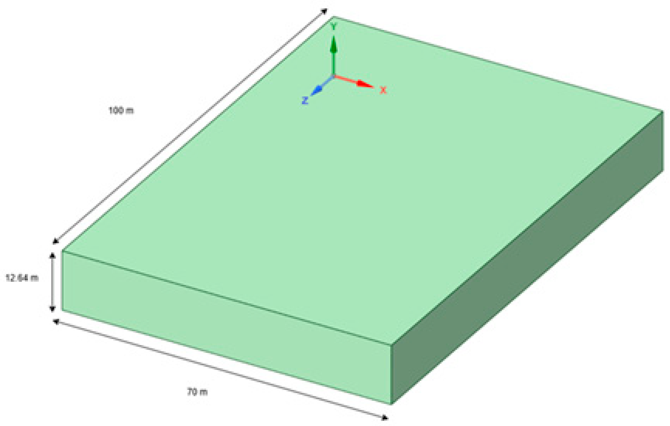
The geometric model represents a 100 m × 70 m segment of Section B of the Salado Estuary in Guayaquil. The geometry and meshing were developed using SpaceClaim and Meshing within ANSYS Workbench 2024 R2. The water depth was set to 9.5 m, assuming a uniform bottom surface. Additionally, a 3.14 m air region above the free surface was included to capture the interaction between the water and air phases.
Figure 2.
Geometric model.
The velocity inlet conditions for water and air were applied as constant velocity boundaries. At the outlet, a gauge pressure of 0 Pa was set, ensuring atmospheric pressure at this boundary, as shown in Figure 3. To account for air-water interaction, surface tension effects were included with a constant coefficient of 0.072 N/m, corresponding to water at room temperature. Additionally, the "Continuum Surface Force" model was implemented to enhance the accuracy of the phase interface representation. Table 1 summarizes the boundary conditions.
2.2. Mesh Independence Analysis
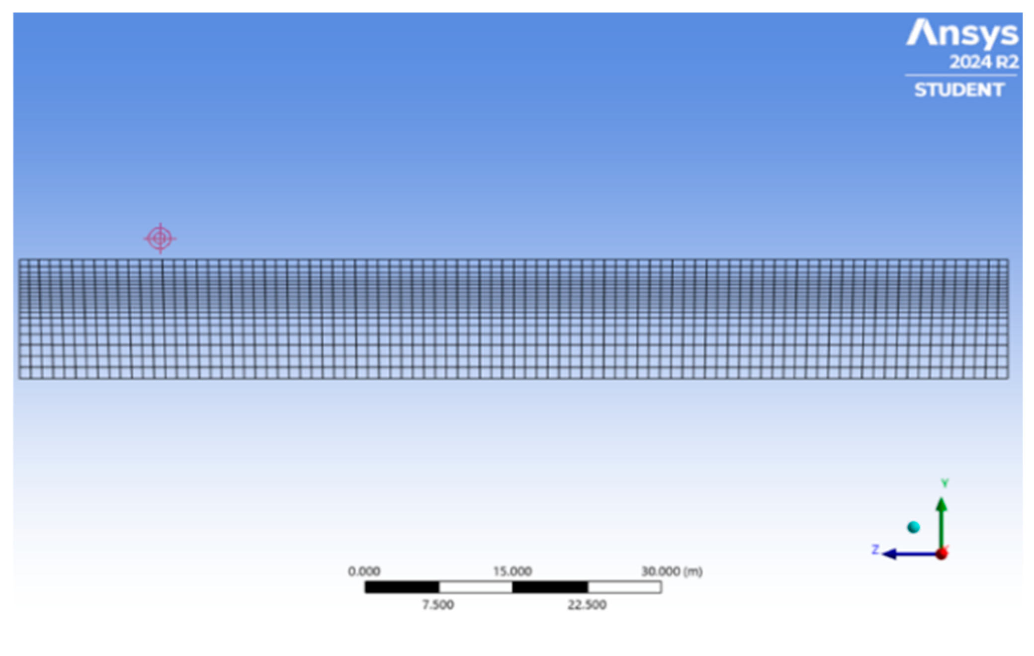
After constructing the geometric model, the next step was mesh generation, which involves discretizing the geometry to accurately capture the physical phenomena in the simulation. To determine an optimal mesh, four different resolutions were tested, containing 105,536, 172,044, 207,328, and 300,300 cells. A convergence analysis was performed, and the mesh with 207,328 tetrahedral cells and 222,500 nodes was selected for the final simulations, as it provided a balance between accuracy and computational efficiency.
Figure 4.
Selected mesh with refinement in the air-water interface.
2.2.1. Control Variable
To evaluate mesh selection, water velocity was measured at the reference point (x: 35 m, y: 9.4 m, z: 0 m), as shown in Figure 5. The results are summarized in Table 2.
As shown in Figure 6, the water velocity at (x: 35 m, y: 9.4 m, z: 0 m) differs by only 0.073% between Mesh 2 and Mesh 3, indicating a negligible variation. In contrast, Mesh 1 and Mesh 4 exhibit more significant deviations from these values.
2.2.2. Overall Quality
The quality of the element of the four generated meshes was studied, the results are summarize in Table 3:
The evaluation of the four generated meshes indicates that Mesh 3 is the most balanced and highest-quality option. It exhibits the highest element quality value (0.66812), signifying a more uniform geometry well-suited for numerical simulations. Additionally, it has the lowest aspect ratio (2.4038), meaning its elements are closer to the ideal shape, reducing potential numerical errors.
The obliquity, which quantifies the angular deviation of elements, is also minimal in Mesh 3 (0.0013479), further confirming its suitability for fluid dynamics calculations. While Mesh 4 achieves the highest orthogonal quality (0.9999)—an important factor for computational accuracy—its other parameters do not perform as well as those of Mesh 3. Given that element quality, aspect ratio, and obliquity are crucial for minimizing discretization errors and ensuring numerical stability, Mesh 3 presents the best overall balance.
Furthermore, these values align with the mesh quality criteria established by Fatchurrohman and Chia [40], reinforcing the robustness of the selected mesh.
2.3. SST Kω Turbulence Model
For the simulations, the k-omega shear stress transport (SST) turbulence model was employed, as it is particularly well-suited for Volume of Fluid (VOF) applications. This model is recognized for its ability to dampen turbulence in interfacial cells, which is crucial for accurately capturing interfacial instabilities [26].
In contrast, the k-ε turbulence model is widely used in engineering due to its robustness and computational efficiency, making it ideal for fully turbulent flows and industrial heat transfer simulations. However, it assumes that molecular viscosity effects are negligible, which limits its accuracy in cases involving adverse pressure gradients or flow separation phenomena. The SST k-ω model overcomes these limitations by combining the high boundary layer accuracy of the k-ω model near walls with the free-stream independence of the k-ε model in the far field.
Originally developed by Menter [41], the SST k-ω model integrates several improvements. One of its key enhancements is the incorporation of a damped cross-diffusion term in the ω equation, which refines the prediction of turbulent viscosity. Additionally, it modifies the definition of turbulent viscosity to enhance the representation of shear stress transport, improving the model's ability to capture complex flow dynamics. The model also includes adjusted modeling constants, ensuring greater accuracy across a wider range of flow conditions.
These improvements make the SST k-ω model significantly more reliable for simulations involving adverse pressure gradients, airfoils, and transonic shock waves, where the standard k-ω model often falls short. Given its ability to balance accuracy near solid boundaries with stability in free-stream regions, the SST k-ω model is an optimal choice for this study.
This model is based on a two-equation system [42], where Equation 1 governs the turbulent kinetic energy (k) and Equation 2 describes the specific turbulence dissipation rate (ω):
2.4. Volume of Fluid Model
It is a numerical method used by CFD to solve problems involving the interaction between fluids, such as air and water. Its main objective is to analyze the volume fraction of fluid within a computational cell.
The volume fraction is represented by α, where a value of 0 indicates the absence of primary fluid in the cell, while a value of 1 indicates its presence [28]
The VOF model is based on the conservation of momentum and continuity, which are described by the Navier-Stokes equations (Equations 3 and 4).
2.4.1. Navier-Stokes Equations
The Navier-Stokes equations are a set of mathematical expressions that describe the behavior of a Newtonian fluid. These equations are derived from the conservation principles of mechanics and thermodynamics applied to a fluid volume. In computational fluid dynamics (CFD), its resolution is carried out by numerical methods implemented in computers.
The Navier–Stokes equations used to analyze the motion of a fluid are [43]:
- Continuity equation
ρ = Fluid Density
= Fluid velocity vector
∇ = Vector differential operator
- Momentum equation
= Viscous stress tensor
F = Force
2.4.2. Open Channel Flow
These flows are known as free-surface flows, as their surface is in direct contact with the atmosphere (e.g., rivers, seas, estuaries, and dams) [44]. They differ from flows in closed pipes due to the influence of pressure; In the case of an open channel, the free surface maintains the same pressure as the atmosphere.
In ANSYS software it is possible to simulate flows in open channels using the VOF method together with the boundary conditions of the free surface [45] This type of model is defined by the Froude number (Equation 5), a dimensionless parameter that relates the inertial force to the hydrostatic force.
Froude's number equation is expressed as:
Where V represents velocity, g is the acceleration due to gravity, and length refers to the depth of the body of water being considered. From this equation, the velocity of the wave can also be calculated, which is defined by:
Flows in open channels are classified according to the number of Froude. Yes < 1, flow is considered subcritical; yes = 1, it is considered critical; what if > 1, The flow is supercritical.
In open-channel flows, there are two key factors in establishing the initial flow conditions:
- Pressure inlet
- Mass Flow rate
The pressure input is given by the following equation:
where:
q is dynamic pressure and is as follows (V, ρ, velocity and density respectively).
is the static pressure and is given as follows (| |, Gravity Unit Vector).
The mass flow rate for channel-to-open flows is represented by the following equation:
where:
ρ is the density and Q the Volumetric flow rate.
Boundary conditions of waves in open channels
2.4.3. Airy Wave Model
The height of the waves (H) is determined as follows:
where A indicates the amplitude of the wave, At is the amplitude at the minimum point and Ac is the amplitude of the wave at the maximum point.
The wave number k is:
The vector wave number is determined from the following equation:
where is the direction of propagation of the reference wave, opposite direction to gravity, indicates the normal direction between and .
Application of wave theory.
To choose the right wave, the following parameters must be followed:
Verification of the total wave regime within the wave break limit.
The relationship between the height of the wave and the depth of the water within the limit of rupture the wave is established as:
The relationship between the wave height and the depth of the wavelength within the breaking limit is established as:
The criterion based on wave theory considers the limit of stability and the breaking of the waves.
Linear waves are described by Airy's wave theory, in which the equations are expressed as follows:
For shallow water, the ratio of wave height to depth to wavelength is set as:
To check the inclination of the waves, the following equation is established:
The equation for checking the relative height of the waves is set as:
The Ursell number is defined as:
The stability criterion of the Ursell number for a linear wave is set as follows:
2.5. Discrete Phase Model
The discrete phase model follows the Euler-Lagrange approach [46] in this method the fluid phase is considered continuous and its resolution is by the Navier-Stoke equations [47] , while the discrete phase is solved by tracing the particles. This model is applied in multiphase simulations where it is desired to analyze the particle path or the interaction between phases.
PET particles were defined with the following properties:

Table 4.
Properties of the MPs particles used in the simulation.
| Microplastic | Density[kg/m3] | Size[mm] |
| Polyethylene Terephthalate (PET) |
1340 | 5 |
The PET particles were injected at two closely spaced locations within the simulation domain, specifically at X = 35 m (Injection 1) and X = 34 m (Injection 2), while maintaining the same coordinates in Y = 9.5 m and Z = 100 m. The injection velocity was set to -0.001 m/s in the Z direction, indicating a downward motion.
Each injection had a flow rate of 0.1 kg/s and a total duration of 450 seconds. The PET particle size was set to 5 mm, as this represents the maximum size defining microplastics (MPs) [48]. The injections followed a single type configuration and were introduced at two distinct points along the X-axis, allowing for a detailed evaluation of the particle trajectory from the inlet to the exit point at the water surface.
2.5.1. Governing Equations in DPM Model
- Balance of forces between particles
The balance of forces equalizes the inertia of particles with the forces acting on it, and is posed as follows:
where is the particle mass, is the phase velocity of the fluid, is the particle velocity, is the particle relaxation time, ρ is the fluid density, is the particle density, is an additional force.
- Discrete Random Walk (DRW) Model
The DRW model, also known as the eddy lifetime model, represents the interaction of particles with a series of discrete turbulent eddies idealized within the fluid phase [49]. Each eddy is characterized by a random velocity fluctuation, distributed in a Gaussian manner, and represented in the three spatial directions as u', v', and w'. This variability in velocity reflects the chaotic nature of turbulent flow. Additionally, the model incorporates the eddy time scale (τₑ), which determines the duration for which a particle remains trapped within an eddy before transitioning to a new one, influencing its trajectory within the turbulent flow.
The values of u', v', and w' that prevail during the lifetime of the turbulent eddy are sampled assuming that they obey a Gaussian probability distribution, establishing as follows:
where ζ represents a random number with a normal distribution, and the rest of the expression on the right side corresponds to the local RMS value of the variations in velocity.
Since the turbulent kinetic energy is known at each point of the flow, it is possible to determine the values of the fluctuating RMS components, assuming that the flow is isotropic, by the following relationship:
For the model k-ε, the model k-ω and their variants. When the simple linear regression model is used, the non-isotropy of the stresses is included in the derivation of the velocity fluctuations.
The characteristic duration of the eddy is defined as a constant:
where is the integral time.
is the random number greater than 0 and less than 1. The random calculation option of produces a more realistic description of the correlation function.
The particle swirl crossing time is defined as:
where is the particle's relaxation time, is the length scale of the eddy and is the magnitude of the relative velocity.
- Saffman's Lift Force
In an investigation on the behavior of a small sphere immersed in a slow-shear flow, it was possible to describe how a moving sphere within a viscous fluid with velocity gradients experiences a lift force oriented perpendicular to the direction of the flow [50].
The mathematical expression that defines Saffman's lifting force is presented as follows:
where K=2.594 and is the strain tensor. This lift force is based on small Reynolds numbers.
The study area exhibits a stable flow with minimal turbulence, which facilitates the definition of initial simulation parameters such as water velocity, wave amplitude, wavelength, water depth, and air velocity, in accordance with previous studies [51,52,53]. Furthermore, the stability of the water indicates the absence of strong currents or significant wind interactions, ensuring consistent flow conditions for the analysis.
- Wave height: 0.01 m
- Wave length: 50 m
- Water depth: 9.5 m
- Water velocity: Simulation A: 0.5 m/s – Simulation B: 1.25 m/s
- Air velocity: 3.3 m/s
2.6. Computational Method
The numerical calculations were performed using Ansys Fluent 2024 R2. The simulation employed standard initialization, starting from the domain inlet. This approach was chosen because flow velocity, pressure, and temperature remain constant throughout the domain. The flat open channel initialization model was applied, as it enhances simulation accuracy in cases where velocity variations are negligible. Additionally, the volumetric fraction was set to 1 at the start, reflecting the presence of fluid in the channel from the beginning.
The simulation ran for 1000 iterations, with a time step of 0.5 seconds and a maximum of 10 iterations per time step, resulting in a total simulated time of 500 seconds. This duration was sufficient to track the trajectory of particles in the open channel flow. However, due to the complexity of the 3D simulation, the computational time averaged 14 hours, significantly increasing the computational cost.
Although the Courant-Friedrichs-Lewy (CFL) number is primarily relevant for explicit methods, it can still serve as a reference for evaluating temporal behavior in implicit simulations. In this case, the CFL number did not significantly impact numerical stability, as implicit methods allow for larger time steps without substantial accuracy loss.
To ensure result accuracy, convergence criteria were established based on the residual values of the simulation. Convergence was considered achieved when residuals dropped below 10⁻⁴, indicating that the system had reached a stable and precise solution. This threshold ensured minimal variation between iterations, providing reliable results aligned with the study’s objectives.
3. Results
Two simulations were conducted to analyze particle dispersion under varying flow conditions, reflecting the natural variability of hydrodynamic parameters. Simulation A was performed with a water inlet velocity of 0.5 m/s, while Simulation B used a higher inlet velocity of 1.25 m/s. This approach allowed for a more realistic assessment of how changes in flow velocity influence particle transport and dispersion.
3.1. Water Velocity Streamlines, Simulation A
Figure 7 illustrates the velocity streamlines in the open channel over time, with a color scale representing speed in meters per second. Darker shades indicate higher velocities (10.83 m/s), while lighter shades correspond to lower velocities (0 m/s).
At 0 seconds (Figure 7a), the flow appears uniform and parallel, with no visible disturbances, indicating that the simulation begins under homogeneous conditions without significant phase interactions. By 100 seconds (Figure 7b), the streamlines maintain a similar pattern, though minor fluctuations start to emerge, possibly due to phase interactions or slight particle dispersion if considered in the study.
At 300 seconds (Figure 7c), the flow remains largely uniform, but subtle changes in velocity distribution suggest that particles, if present, may begin to move more noticeably or settle. By 500 seconds (Figure 7d), the flow pattern is more developed, with potential variations in particle velocity and distribution, influenced by fluid viscosity, emerging turbulence, or sedimentation.
Overall, the analysis confirms that the flow remains stable throughout the domain, with no significant eddies or abrupt disturbances.
3.2. Water Velocity Streamlines, Simulation B
Figure 8 illustrates the flow evolution considering a water inlet velocity of 1.25 m/s. The highest velocities, around 4.16 m/s, are shown in dark tones, while the lowest, near 0 m/s, appear in lighter shades.
At the initial time step (Figure 8a), the flow is uniform and well-aligned, indicating homogeneous initial conditions with no significant phase interactions. By the second stage (Figure 8b), minor variations in the streamlines emerge, potentially due to phase interactions or the initial stages of particle dispersion, if applicable.
In Figure 8c, the flow remains predominantly stable, though slight changes in velocity distribution suggest gradual particle displacement or the onset of sedimentation. By the final stage (Figure 8d), more noticeable modifications in the flow pattern appear, including velocity variations and possible turbulence or sedimentation effects influenced by fluid viscosity.
Overall, the flow remains stable within the simulation domain, with no abrupt disturbances or large eddy formations.
3.3. Density Contours
Throughout the simulated time intervals, the interface between water and air remains stable and uniform across the entire computational domain. Figure 9a, 9b, and 9c illustrate this consistency, with a clear distinction between the two phases. The density scale highlights these differences, where blue tones represent higher-density regions corresponding to water, while red tones indicate lower-density areas associated with air.
The flow behavior aligns with the characteristics of a channel with minimal disturbances and low velocities in both phases. No significant variations in the interface or flow pattern are observed, reinforcing the stability of the system.
These results confirm the accuracy of the simulation in representing the expected behavior of the phases under the given conditions, demonstrating a successful numerical reproduction of open-channel flow stability.
3.4. Pressure Contours
Figure 10 illustrates the pressure stability characteristics of estuaries and open channels. Across the entire domain, air pressure remains constant until it reaches the liquid’s bottom, where the highest pressure values are recorded. This pressure distribution remains consistent in all analyzed instances, specifically at 0 s, 100 s, 300 s, and 500 s.
3.5. Air-Water Interface
The iso-surface captured in Figure 11 appears predominantly blue, indicating that the visualized region primarily corresponds to the aqueous domain, with minimal air presence in that layer. This suggests that water is the dominant fluid in this region of the interface, aligning with the expected configuration of a salt estuary. The variations observed on the surface result from surface instabilities caused by wave effects within the water body. These waves introduce minor disturbances that slightly alter the interface shape without significantly impacting the overall flow dynamics.
Overall, the simulation exhibits a relatively stable flow state, with a well-defined air-water interface and minimal fluctuations in phase distribution. This stability suggests that the simulated conditions accurately reflect the typical dynamics of a salt estuary under normal conditions.
3.6. Particle Dispersal
Likewise, two simulations were carried out with a change in velocity, Simulation A was performed with a water inlet velocity of 0.5 m/s, while Simulation B used a higher inlet velocity of 1.25 m/s. The following results were obtained:
3.6.1. Particle Dispersal for Water Inlet Velocity of 0.5 m/s
In the analysis of PET particle tracking during simulation A, the particles exhibit distinct behavior throughout the process. Initially, as shown in Figure 12a-d, the particles follow a linear trajectory, indicating that they fall into the water shortly after injection. As observed in Figure 12d, the particles reach the bottom of the computational domain and continue to move along the bottom surface, influenced by drag forces.
Figure 12e-g demonstrate that the particles maintain the same trajectory, progressing toward the end of the domain. By Figure 12h, the particles exit the computational domain, signaling the completion of the tracking process at approximately 175 seconds.
In the subsequent time steps, as seen in Figure 12i and 12j, the particles continue along their established path without significant deviations. By Figure 12k, it is evident that the particle injection process is complete, as the predefined injection time of 450 seconds has elapsed. Finally, in Figure 12l, the particles continue to move within the domain, consistently guided by drag forces, indicating the persistence of the flow dynamics over time.
In the analysis of simulation A, as shown in Figure 13, the particle trajectories exhibit minimal variation across the different evaluated scenarios. This indicates that the flow velocity remains consistent, maintaining predictable behavior throughout the domain. The particles follow an inclined path from the injection point, gradually descending due to gravity until they settle at the bottom of the domain. They reach a depth between 18 and 22.5 meters along the z-direction, suggesting that the sedimentation process is gradual and steady under the defined conditions. The time required for the PET particles to travel the entire length of the domain is approximately 200 seconds, further supporting the notion of a stable flow velocity that remains constant over both time and space. This indicates a controlled flow pattern with no significant fluctuations.
The uniformity in the particle trajectories suggests the absence of significant turbulence or unexpected phase interactions, pointing to a stable multiphase flow in controlled equilibrium.
3.6.2. Particle Dispersal for Water Inlet Velocity of 1.25 m/s
Figure 14a-d illustrate the initial stages of PET particle tracking in simulation B, viewed isometrically. Shortly after injection, the particles enter the water and begin to drift. In Figure 14c, the particles reach the bottom of the computational domain at approximately half of their length. As shown in Figure 14d, they continue to advance through the domain, driven by drag forces. Figure 14e demonstrates that the PET particles reach the end of the domain after 100 seconds. In Figure 14f, 14g, and 14h, the particles follow their expected trajectory, consistent with the selected simulation parameters.
In the subsequent time steps, as shown in Figure 14i and 14j, the particles maintain their motion with no significant changes. By Figure 14k, the completion of particle injection is confirmed, as the injection time was set at 450 seconds. Finally, Figure 14l shows a decrease in the number of particles within the domain, which is attributed to their velocity.
Figure 15 shows the evolution of the PET particle trajectories in simulation B, from their injection into the water body at a depth of approximately 9.5 meters. As the particles move through the domain, they exhibit a steady, gradual descent until reaching the bottom of the computational domain, which occurs between 50 and 60 meters along the z-axis. This continuous descent pattern suggests a progressive sedimentation process, with no abrupt changes or irregular deviations in the particle trajectories. The observed stability can be attributed to the conditions within the estuary, where turbulence is minimal, fostering a stable flow environment. The low turbulence allows the particles to maintain a consistent motion, unaffected by random forces that might otherwise disrupt their paths.
Regarding the transit time, it is estimated that a PET particle takes approximately 80 seconds to travel 100 meters along the domain. This time is consistent with a controlled flow, where the particles maintain a constant velocity from injection to exit. The combination of the gradual descent and consistent travel time further supports the idea of a flow environment with low dynamic complexity.
4. Discussion
4.1. Influence of Water Velocity on Particle Dispersal
A comparison of simulations A and B reveals key differences in the behavior of PET particles in the Salado Estuary, particularly in terms of sedimentation distances and particle trajectories. These differences highlight the influence of flow conditions and domain properties on particle behavior.
In simulation A (Figure 13), PET particles settle at the bottom of the estuary between 18 and 22.5 meters from their injection point. In contrast, in simulation B (Figure 15), particles reach the bottom between 50 and 60 meters along the longitudinal axis of the estuary. This difference suggests that horizontal transport plays a more significant role in simulation B, allowing particles to travel a greater distance before settling. This is attributed to the higher water flow velocity in simulation B.
Despite these differences in sedimentation distances, both simulations show uniform particle trajectories with minimal variations, owing to the low turbulence in the estuary. The stable flow conditions facilitate controlled particle transport, ensuring that the particles follow a predictable path from injection to bottom sedimentation.
Regarding domain exit time, a PET particle in simulation A takes approximately 200 seconds to exit the domain, whereas in simulation B, it takes just 80 seconds. This difference supports the hypothesis that higher water velocities accelerate the transport of MPs, reducing their residence time in the aquatic environment and potentially influencing their accumulation further from the emission point.
A Pearson correlation analysis was conducted to assess the relationship between water velocity and the distance traveled by MPs before reaching the domain’s bottom. The analysis reveals a strong positive correlation (r = 0.97) [54], indicating that as water velocity increases, MPs travel greater distances before settling.
These findings emphasize the need for further studies that consider factors such as variations in MP density, interactions with biofilms, and degradation processes, all of which could significantly affect MP behavior in the aquatic environment. Additionally, future research could focus on more complex turbulence models and experimental validations under real-world conditions to better represent these dynamics.
4.2. Comparison with Previous Studies
The results of the present research can be compared to similar studies involving simulations and experimental measurements of particle dispersion in aquatic systems. Previous research has shown that particle dispersion is influenced not only by the water flow velocity but also by dynamic conditions such as waves, eddy formation, wind-induced turbulence, and interactions with natural or man-made structures.
Quyen and Choi [27] emphasize that the physical properties of particles, including size and density, significantly affect their dispersion in the presence of artificial structures. Small particles (0.2 mm) exhibit high dispersion due to vertical mixing, while larger, denser particles tend to sink rapidly without being suspended. In contrast to their findings, the present study shows that the particles maintain a uniform flow pattern, with limited interaction between particles and the flow, due to the absence of velocity gradients generated by structures.
Quyen et al. [28] investigated the effects of different types of coastal breaks on the behavior of MPs. Lighter particles experience forward advection in the surface layer, while neutral and heavier particles move toward the bottom or inshore, influenced by larger wave sizes than those considered in the present study. In contrast, the present simulation does not account for such variations in size and density, as dynamic conditions such as waves or undertows are not included.
Fatahi et al. [26] analyze the impact of water velocity, particle size, and density on the distribution of particulate matter in coastal environments. Their findings show that PET particles tend to settle on the bottom in low-velocity waters, similar to the behavior observed in the current study, where PET particles travel along the domain before reaching the estuary's bottom. Denser particles, like PET and PU, tend to sink in slow-moving water, while lighter particles, such as PP, remain at the surface and are transported to shore. Fatahi et al. also noted that as water velocity increases, lighter particles travel greater distances, underscoring the importance of velocity in dispersion.
Kabir et al. [24] observed that water velocity directly influences the moment particles reach the bottom of the domain. At velocities of 0.1 m/s and 0.3 m/s, larger and denser particles tend to settle near the entrance, while smaller particles remain suspended longer and are transported further. In contrast, the present study, with water velocities of 0.5 m/s and 1.25 m/s in the Estero Salado, shows that MPs travel greater distances before settling. This indicates that in bodies of water with minimal wave activity, increased water velocity results in longer transport distances before deposition. These differences can be attributed to the specific hydrodynamic conditions and the nature of the water body studied, emphasizing the importance of considering environmental characteristics when analyzing MP dispersion.
The current simulations provide a controlled environment that allows for the observation of basic patterns in MP transport and sedimentation. In contrast, the studies reviewed incorporate additional factors such as artificial structures, waves, and velocity variations, leading to more dynamic and diverse particle behaviors. This research complements the present analysis by offering a broader perspective on the processes influencing the dispersion and accumulation of MPs in different aquatic environments.
5. Conclusions
The literature review provided valuable insights into how key characteristics of MP particles, such as size and density, influence their transport and sedimentation in aquatic environments. This understanding was essential for configuring and analyzing the simulations conducted in the study.
Based on this theoretical framework, the geometry and meshing of section B of the Salado Estuary were designed, reflecting its specific conditions, including a depth of 9.5 meters, a length of 100 meters, and a width of 70 meters.
During the simulation analysis, density contours and particle trajectories were employed to visualize the distribution and movement of MP particles throughout the flow. Density contours helped identify particle concentrations in various areas, while particle traces illustrated individual movements, facilitating a better understanding of MP dispersion and deposition within the estuary.
The primary factor influencing the simulation results was the water inflow velocity. As the velocity increased, particles traveled greater distances from the injection point before settling, delaying sedimentation. In simulation A, with lower flow velocity, particles descended more quickly due to reduced horizontal drag forces. In contrast, simulation B, with a higher flow velocity, demonstrated a more dominant horizontal transport, which slowed sedimentation. This highlights the critical role of water velocity in the transport and distribution of MPs in the Salado Estuary.
To refine the analysis, future simulations should vary the average water velocity and incorporate additional environmental and operational factors, such as water turbidity and channel geometry. This would allow for a more comprehensive evaluation of MP dispersion, transport, and deposition. A sensitivity analysis could also help identify the most influential factors affecting MP dispersion, further optimizing the model and enhancing the understanding of MP behavior in riverine environments.
This study contributes valuable knowledge on MP trajectory and sedimentation, emphasizing the impact of water velocity on MP behavior in estuarine environments. It also advances the understanding of MP dynamics in the Salado Estuary, aiding in future environmental assessments and mitigation strategies in the inner and outer estuary of the Gulf of Guayaquil due to its importance for the fishing and aquaculture sector. However, there are limitations, particularly the need for experimental validation to corroborate simulation results. Future research could expand on this work by investigating the behavior of smaller MP particles, incorporating wind effects, tidal, and evaluating the impact of different particle shapes and compositions. Comparing numerical simulations with field data would also improve the model's accuracy and applicability to real-world estuarine systems.
Author Contributions
Conceptualization, L.V., M.C.; methodology, L.V., J.F. and A.M..; software, J.F. and A.M..; validation, J.F. and A.M.; formal analysis, L.V.; investigation, J.F. and A.M..; data curation, J.F. and A.M..; writing—original draft preparation, J.F. and A.M..; writing—review and editing, L.V., M.C..; visualization, L.V., J.F. and A.M.; supervision, L.V.. All authors have read and agreed to the published version of the manuscript.
Funding
This research received no external funding.
Conflicts of Interest
The authors declare no conflict of interest.
References
- Priya, A.K.; Jalil, A.A.; Dutta, K.; Rajendran, S.; Vasseghian, Y.; Qin, J.; et al. Microplastics in the environment: Recent developments in characteristic, occurrence, identification and ecological risk. Chemosphere, vol. 298, p. 134161, 2022. [CrossRef]
- Pothiraj, C.; Gokul, T.A.; Kumar, K.R.; Ramasubramanian, A.; Palanichamy, A.; Venkatachalam, K.; et al. Vulnerability of microplastics on marine environment: A review. Ecological Indicators, vol. 155, p. 111058, 2023. [CrossRef]
- Thushari, G.G.N.; Senevirathna, J.D.M. Plastic pollution in the marine environment. Heliyon, vol. 6, n.o 8, p. e04709, 2020. [CrossRef]
- Nawab, A.; Ahmad, M.; Khan, M.T.; Nafees, M.; Khan, I.; Ihsanullah, I. Human exposure to microplastics: A review on exposure routes and public health impacts. Journal of Hazardous Materials Advances, vol. 16, p. 100487, 2024. [CrossRef]
- Pernia, B.; Mero, M.; Cornejo, X.; Zambrano, J. IMPACTOS DE LA CONTAMINACIÓN SOBRE LOS MANGLARES DE ECUADOR. In 2019. p. manglaresdeamerica.com/index.php/ec/issue/view/2.
- Sharma, S.; Basu, S.; Shetti, N.P.; Nadagouda, M.N.; Aminabhavi, T.M. Microplastics in the environment: Occurrence, perils, and eradication. Chemical Engineering Journal, vol. 408, p. 127317, 2021. [CrossRef]
- Boucher, J.; Friot, D. Primary Microplastics in the Oceans: A Global Evaluation of Sources. 2017. [CrossRef]
- Bikiaris, N.; Nikolaidis, N.F.; Barmpalexis, P. Microplastics (MPs) in Cosmetics: A Review on Their Presence in Personal-Care, Cosmetic, and Cleaning Products (PCCPs) and Sustainable Alternatives from Biobased and Biodegradable Polymers, Cosmetics, vol. 11, n.o 5, 2024. [CrossRef]
- Maleka, T.; Greenfield, R.; Muniyasamy, S.; Modley, L.A. An overview on the characterization of microplastics (MPs) in waste water treatment plants (WWTPs). Sustainable Water Resources Management, vol. 10, n.o 5, oct. 2024. [CrossRef]
- Hoang, V.H.; Nguyen, M.K.; Hoang, T.D.; Ha, M.C.; Huyen, N.T.T.; Bui, V.K.H.; et al. Sources, environmental fate, and impacts of microplastic contamination in agricultural soils: A comprehensive review. Science of The Total Environment, vol. 950, p. 175276, 2024. [CrossRef]
- Hartmann, N.; Rist, S.; Bodin, J.; Jensen, L.; Schmidt, S.; Mayer, P.; et al. Microplastics as vectors for environmental contaminants: Exploring sorption, desorption, and transfer to biota: Microplastics as Contaminant Vectors: Exploring the Processes. Integrated Environmental Assessment and Management, vol. 13, pp. 488-493, ene. 2017. [CrossRef]
- Sutkar, P.R.; Gadewar, R.D.; Dhulap, V.P. Recent trends in degradation of microplastics in the environment: A state-of-the-art review. Journal of Hazardous Materials Advances, vol. 11, p. 100343, 2023. [CrossRef]
- Matavos-Aramyan, S. Addressing the microplastic crisis: A multifaceted approach to removal and regulation. Environmental Advances, vol. 17, p. 100579, 2024. [CrossRef]
- Duis, K.; Coors, A. Microplastics in the aquatic and terrestrial environment: sources (with a specific focus on personal care products), fate and effects. Environmental Sciences Europe, vol. 28, n.o 1, pp. 1-25, dic. 2016. [CrossRef]
- Picó, Y.; Barceló, D. Analysis and prevention of microplastics pollution in water: Current perspectives and future directions. ACS Omega, vol. 4, n.o 4, pp. 6709-6719, abr. 2019. [CrossRef]
- Demirel, B.; Yaraş, A.; ELÇİÇEK, H. Crystallization Behavior of PET Materials. Balıkesir Üniversitesi Fen Bilimleri Enstitü Dergisi, vol. 13, pp. 26-35, ene. 2011.
- Anis, A.; Elnour, A.Y.; Alhamidi, A.; Alam, M.A.; Al-Zahrani, S.M.; AlFayez, F.; et al. Amorphous Poly(ethylene terephthalate) Composites with High-Aspect Ratio Aluminium Nano Platelets, Polymers, vol. 14, n.o 3, 2022. [CrossRef]
- Kianfar, E. Polyethylene terephthalate (PET) Recycling: A Review". Case Studies in Chemical and Environmental Engineering, feb. 2024. [CrossRef]
- Kovačić, M.; Tomić, A.; Tonković, S.; Pulitika., A.; Papac Zjačić, J.; Katančić, Z. et al. Pristine and UV-Weathered PET Microplastics as Water Contaminants: Appraising the Potential of the Fenton Process for Effective Remediation, Processes, vol. 12, n.o 4, 2024. [CrossRef]
- Adediran, G.A.; Cox, R.; Jürgens, M.D.; Morel, E.; Cross, R.; Carter, H.; et al. Fate and behaviour of Microplastics (> 25µm) within the water distribution network, from water treatment works to service reservoirs and customer taps. Water Research, vol. 255, p. 121508, 2024. [CrossRef]
- Pittroff, M.; Müller, Y.K.; Witzig, C.S.; Scheurer, M.; Storck, F.R.; Zumbülte, N. Microplastic analysis in drinking water based on fractionated filtration sampling and Raman microspectroscopy. Environmental Science and Pollution Research, vol. 28, n.o 42, pp. 59439-59451, nov. 2021. [CrossRef]
- Oßmann, B.E.; Sarau, G.; Holtmannspötter, H.; Pischetsrieder, M.; Christiansen, S.H; Dicke, W. Small-sized microplastics and pigmented particles in bottled mineral water. Water Research, vol. 141, pp. 307-316, 2018. [CrossRef]
- Shruti, V.C.; Pérez-Guevara, F.; Elizalde-Martínez, I.; Kutralam-Muniasamy, G. First study of its kind on the microplastic contamination of soft drinks, cold tea and energy drinks - Future research and environmental considerations. Science of The Total Environment, vol. 726, p. 138580, 2020. [CrossRef]
- Kabir, S.M.A.; Bhuiyan, M.A.; Zhang, G.; Pramanik, B.K. Use of computational fluid dynamics to model microplastic transport in the stormwater runoff system. Process Safety and Environmental Protection, vol. 196, p. 106873, 2025. [CrossRef]
- Ioakeimidis, C.; Fotopoulou, K.N.; Karapanagioti, H.K.; Geraga, M.; Zeri, C.; Papathanassiou, E.; et al. The degradation potential of PET bottles in the marine environment: An ATR-FTIR based approach. Sci Rep, vol. 6, p. 23501, mar. 2016. [CrossRef]
- Fatahi, M.; Akdogan, G.; Dorfling, C.; Van Wyk, P. Numerical study of microplastic dispersal in simulated coastal waters using cfd approach. Water (Switzerland), vol. 13, n.o 23, dic. 2021. [CrossRef]
- Quyen, L.D.; Choi, J.M. Accumulation and Dispersion of Microplastics near A Submerged Structure: Basic Study Using A Numerical Wave Tank. Journal of Marine Science and Engineering, vol. 10, n.o 12, dic. 2022. [CrossRef]
- Quyen, L.D.; Park, Y.G.; Lee, I.C.; Choi, J.M. CFD Analysis of Microplastic Transport over the Slopes. Journal of Marine Science and Engineering, vol. 12, n.o 1, ene. 2024. [CrossRef]
- Dichgan, F.; Boos, J.P.; Ahmadi, P.; Frei, S.; Fleckenstein, J.H. Integrated numerical modeling to quantify transport and fate of microplastics in the hyporheic zone. Water Research, vol. 243, n.o 12 0349, 2023, Accedido: 14 de septiembre de 2024 [En línea] Disponible en:. [Google Scholar] [CrossRef]
- Ding, Y.; Liu, H.; Yang, W. Numerical prediction of the short-term trajectory of microplastic particles in Laizhou Bay. Water (Switzerland), vol. 11, n.o 11, nov. 2019. [CrossRef]
- Molazadeh, M.; Liu, F.; Simon-Sánchez, L.; Vollersten, J. Buoyant microplastics in freshwater sediments – How do they get there? Science of the Total Environment, vol. 860, feb. 2023. [CrossRef]
- Arias, P. Los desechos se acumulan en ramales del Salado sin que nadie actúe o sancione. Expreso, Guayaquil, 26 de marzo de 2023. Accedido: 14 de septiembre de 2024. [En línea]. Disponible en: https://www.expreso.ec/guayaquil/desechos-acumulan-ramales-salado-nadie-actue-sancione-155217.html.
- Sarria, R.; Gallo, J. Microplasticos. Journal de Ciencia e Ingeniería, vol. 8, n.o 1, pp. 21-27, 2016.
- Islam, M.M.; Rayhan, A.B.M.S.; Wang, J.; Shamim, M.A.H.; Ke, H.; Wang, C. et al. Tracing microplastics in marine fish: Ecological threats and human exposure in the Bay of Bengal. Science of The Total Environmen, vol. 963, p. 178462, 2025. [CrossRef]
- Meroney, R.; Ohba, R.; Leitl, B.; Kondo, H.; Grawe, D.; Tominaga, Y. Review of CFD guidelines for dispersion modeling. Fluids, vol. 1, n.o 2, jun. 2016. [CrossRef]
- Hu, H. Computational Fluid Dynamics, 2012, pp. 421-472. [CrossRef]
- Szpicer, A.; Bińkowska, W.; Stelmasiak, A.; Zalewska, M.; Wojtasik-Kalinowska, I.; Piwowarski, K.; et al. Computational Fluid Dynamics Simulation of Thermal Processes in Food Technology and Their Applications in the Food Industry. Applied Sciences, vol. 15, n.o 1, 2025. [CrossRef]
- Mcnay, J.; Hilditch, R. Evaluation of Computational Fluid Dynamics (CFD) vs. Target Gas Cloud for Indoor Gas Detection Design. Journal of Loss Prevention in the Process Industries, vol. 50, pp. 75-79, 2017. [CrossRef]
- de Fretes, R.; Djatmiko, E.; Wardhana, W. Hydrodynamic analysis of additional effect of submarine appendages. Advances and Applications in Fluid Mechanics, vol. 13, ene. 2013.
- Fatchurrohman, N.; Chia, S.T. Performance of hybrid nano-micro reinforced mg metal matrix composites brake calliper: Simulation approach, en IOP Conference Series: Materials Science and Engineering, Institute of Physics Publishing, nov. 2017. [CrossRef]
- Menter, F.R. Two-equation eddy-viscosity turbulence models for engineering applications. AIAA Journal, vol. 32, pp. 1598-1605, 1994.
- Younoussi, S.; Ettaouil, A. Calibration method of the k-ω SST turbulence model for wind turbine performance prediction near stall condition. Heliyon, vol. 10, n.o 1, ene. 2024. [CrossRef]
- Barba, L.; Forsyth, G. CFD Python: the 12 steps to Navier-Stokes equations. Journal of Open Source Education, vol. 1, p. 21, nov. 2018. [CrossRef]
- Chanson, H. 1 - Introduction. In: Chanson H, editor. Hydraulics of Open Channel Flow (Second Edition) [Internet]. Second Edition. Oxford: Butterworth-Heinemann, 2004, pp. 3-8. [CrossRef]
- Mohsin, M.; Kaushal, D.R. Three-dimensional computational fluid dynamics (volume of fluid) modelling coupled with a stochastic discrete phase model for the performance analysis of an invert trap experimentally validated using field sewer solids. Particuology, vol. 33, pp. 98-111, 2017. [CrossRef]
- Padding, J.; Deen, N.; Peters, E.A.J.F.; Kuipers, H. Euler–Lagrange Modeling of the Hydrodynamics of Dense Multiphase Flows. In: Advances in Chemical Engineering, vol. 46, 2015, pp. 137-191. [CrossRef]
- Oroná, J.D.; Zorrilla, S.E.; Peralta, J.M. Computational fluid dynamics combined with discrete element method and discrete phase model for studying a food hydrofluidization system. Food and Bioproducts Processing, vol. 102, pp. 278-288, 2017. [CrossRef]
- Li, Y.; Chen, L.; Zhou, N.; Chen, Y.; Ling, Z.; Xiang, P. Microplastics in the human body: A comprehensive review of exposure, distribution, migration mechanisms, and toxicity. Science of The Total Environment, vol. 946, p. 174215, 2024. [CrossRef]
- Gosman, A. ~D.; Ioannides, E. Aspects of computer simulation of liquid-fueled combustors. Journal of Energy, vol. 7, pp. 482-490, dic. 1983.
- Saffman, P.G. The lift on a small sphere in a slow shear flow. Journal of Fluid Mechanics, vol. 22, n.o 2, pp. 385-400, 1965. [CrossRef]
- Alcaldía de Guayaquil. NAVEGABILIDAD EN EL RIO GUAYAS JUNIO 2017. 2017.
- Twilley, R.; Cárdenas, W.; Rivera-Monroy, V.; Espinoza, J.; Suescum, R.; Armijos, M.; et al. The Gulf of Guayaquil and the Guayas River Estuary, Ecuador, vol. 144, 2001, pp. 245-263. [CrossRef]
- JAVIER, R.; Coell, S. ESTUDIO DE CASO ENERGÍA EÓLICA PARA GENERACIÓN DE ENERGÍA ELÉCTRICA A NIVEL URBANO, PhD Thesis, 2024. [CrossRef]
- Selvanathan, M.; Jayabalan, N.; Saini, G.; Supramaniam, M.; Hussain, N. Employee Productivity in Malaysian Private Higher Educational Institutions. PalArch’s Journal of Archaeology of Egypt/ Egyptology, vol. 17, pp. 66-79, oct. 2020. [CrossRef]
Figure 1.
Study area: 2°10'53"S 79°54'03"W; 2°10'50"S 79°54'05"W; 2°10'54"S 79°54'05"W; 2°10'51"S 79°54'07"W.
Figure 1.
Study area: 2°10'53"S 79°54'03"W; 2°10'50"S 79°54'05"W; 2°10'54"S 79°54'05"W; 2°10'51"S 79°54'07"W.
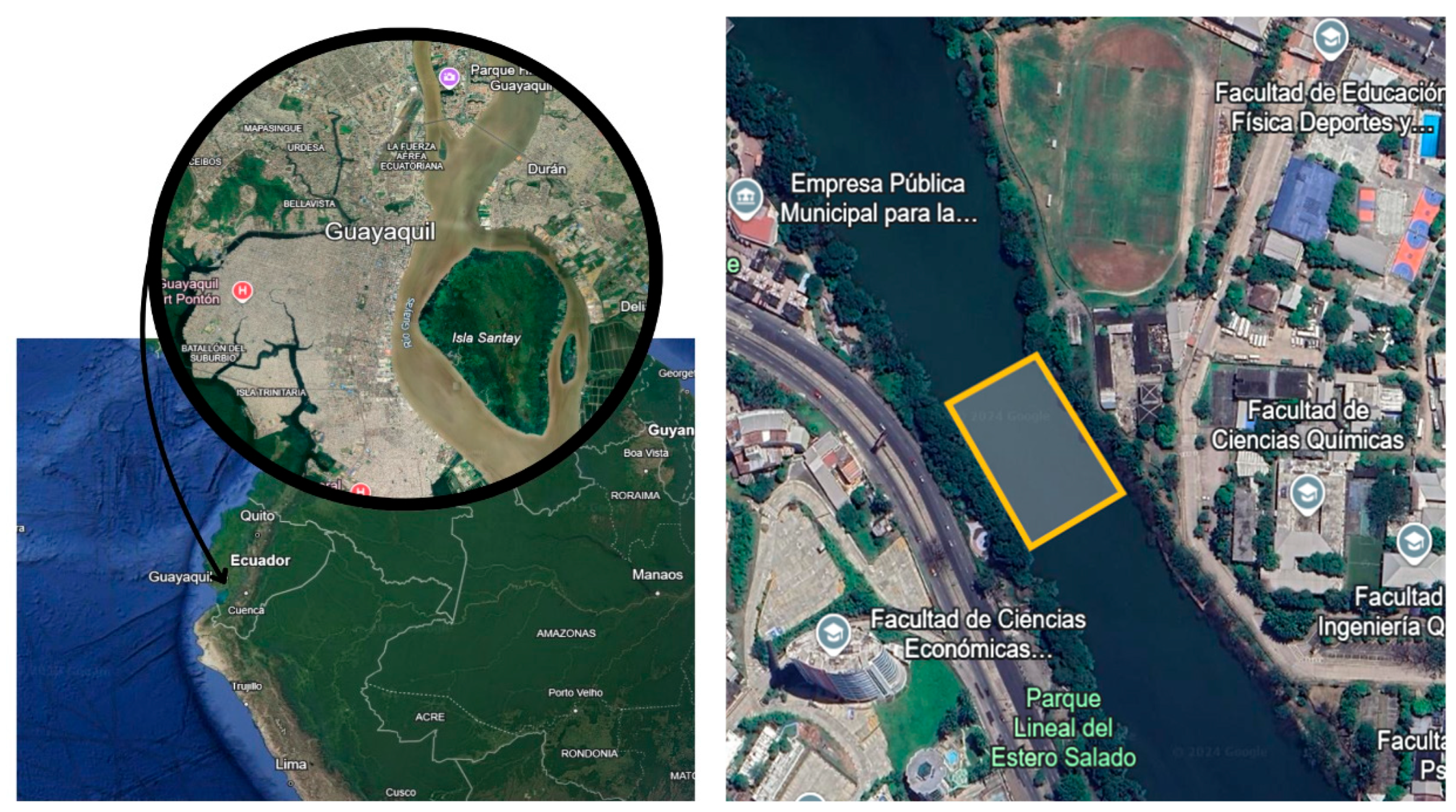
Figure 3.
Domain boundary conditions.
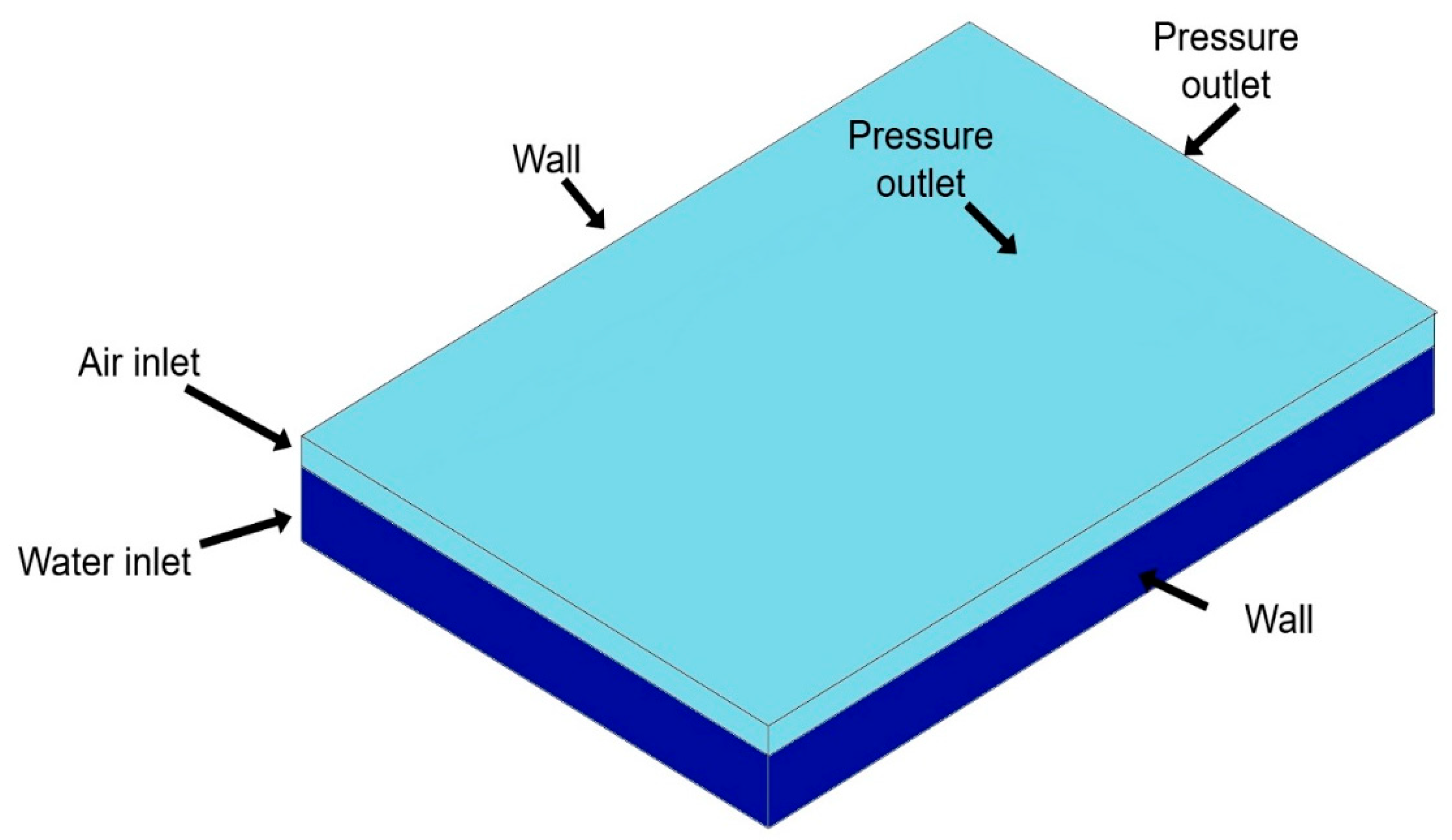
Figure 5.
Velocity streamlines and reference point for different mesh resolutions.
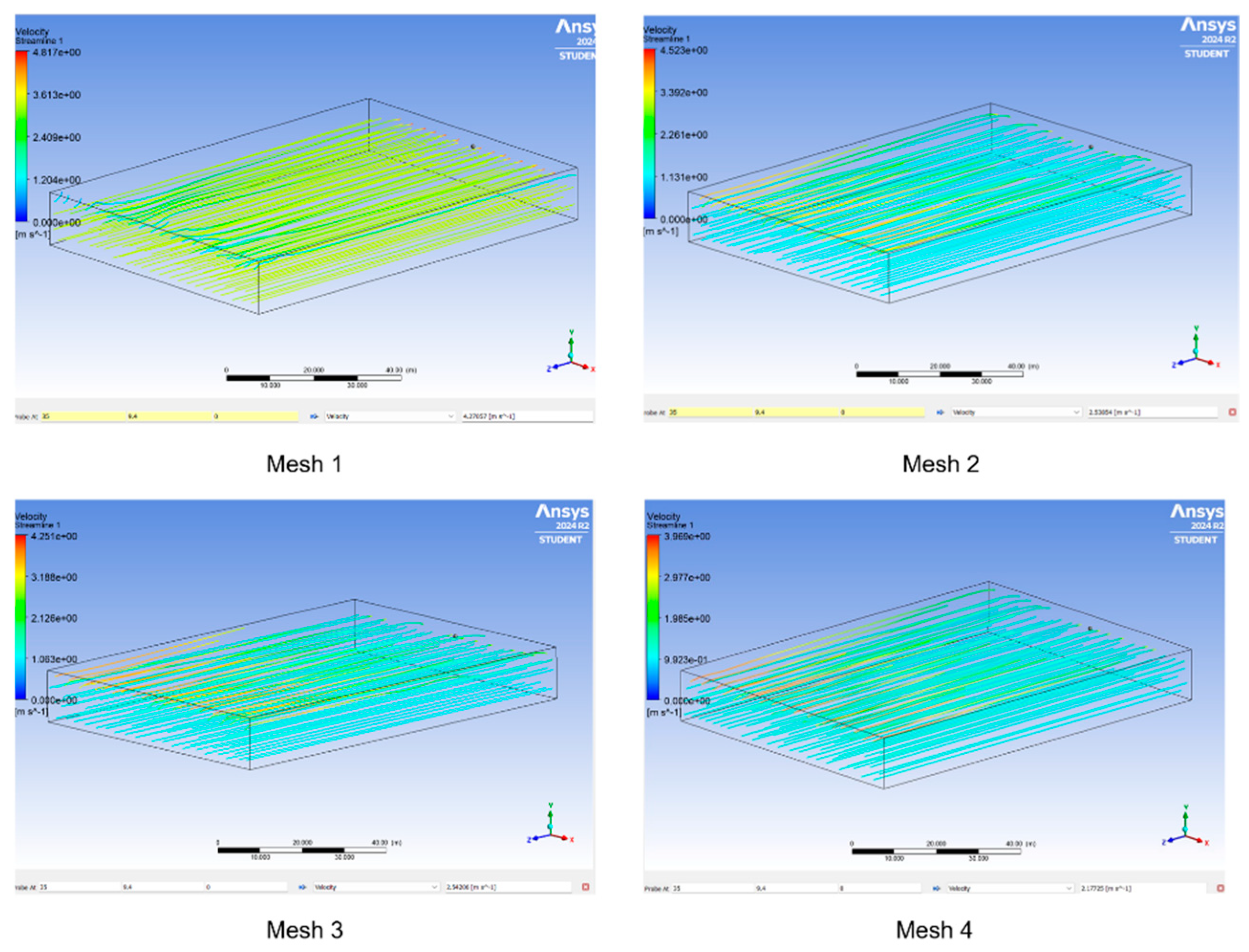
Figure 6.
Water velocity at the reference point for different mesh resolutions.
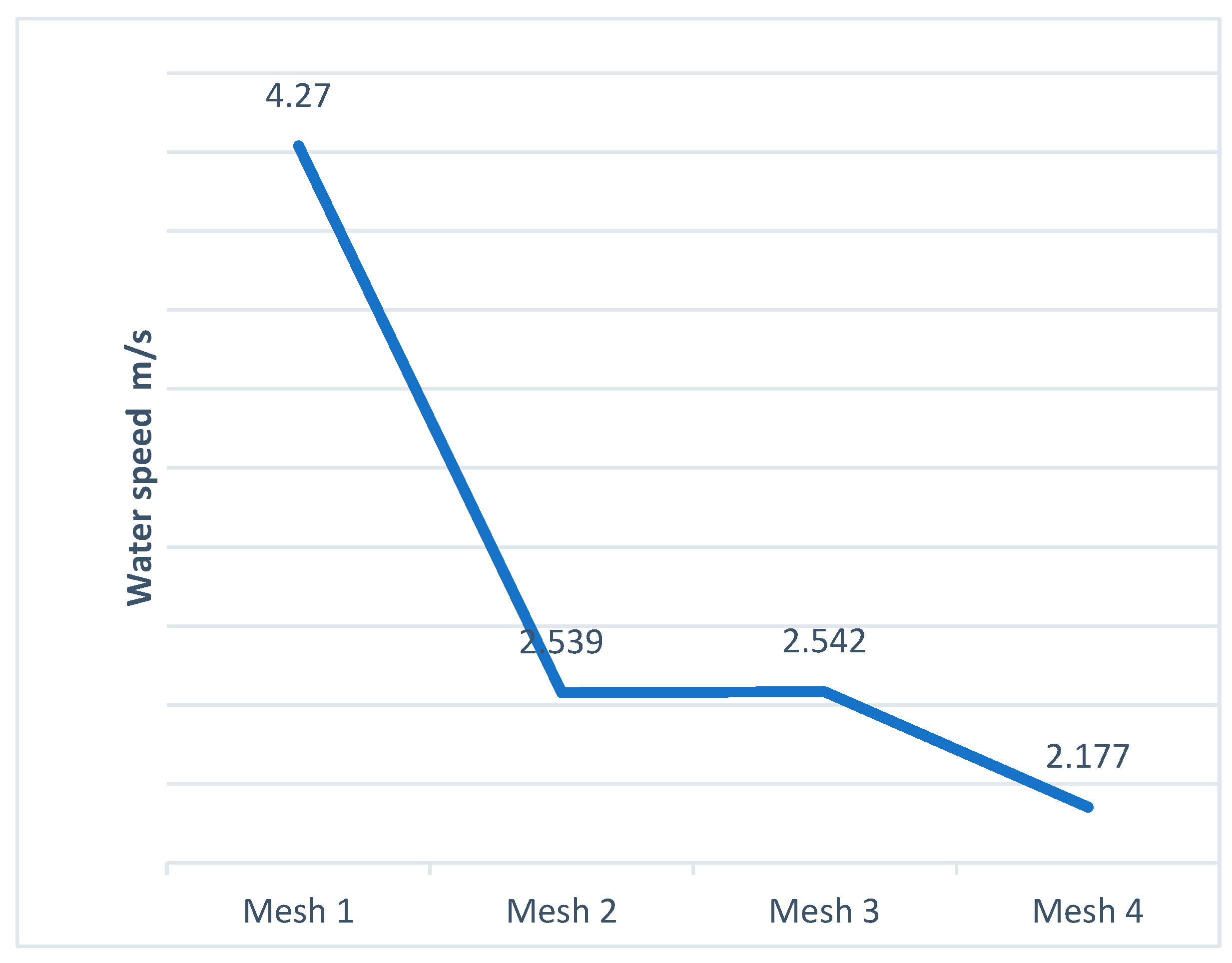
Figure 7.
Water velocity streamlines in Simulation A at different time steps: (a) 0 s, (b) 100 s, (c) 300 s, and (d) 500 s.
Figure 7.
Water velocity streamlines in Simulation A at different time steps: (a) 0 s, (b) 100 s, (c) 300 s, and (d) 500 s.
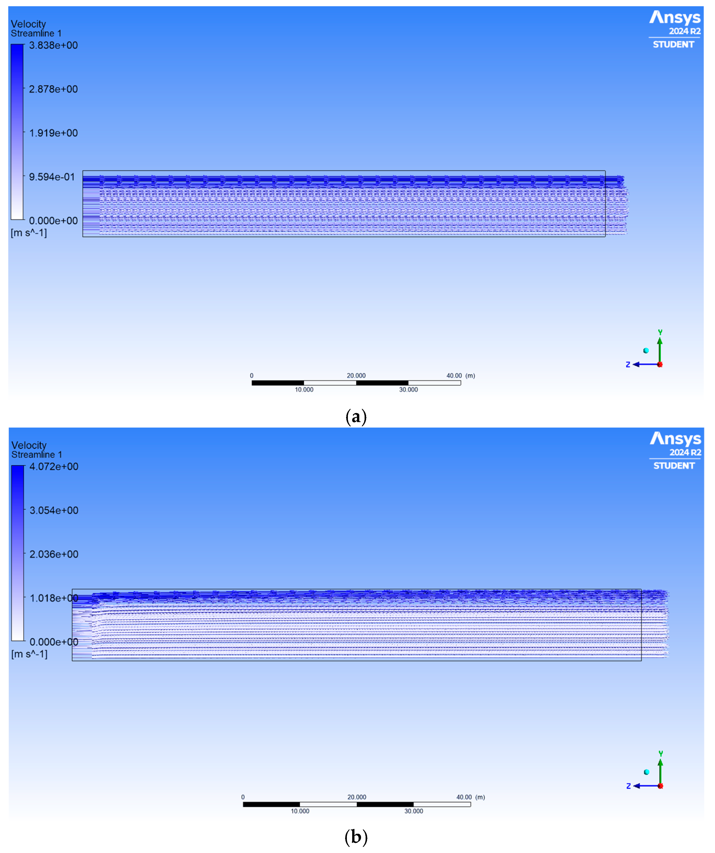
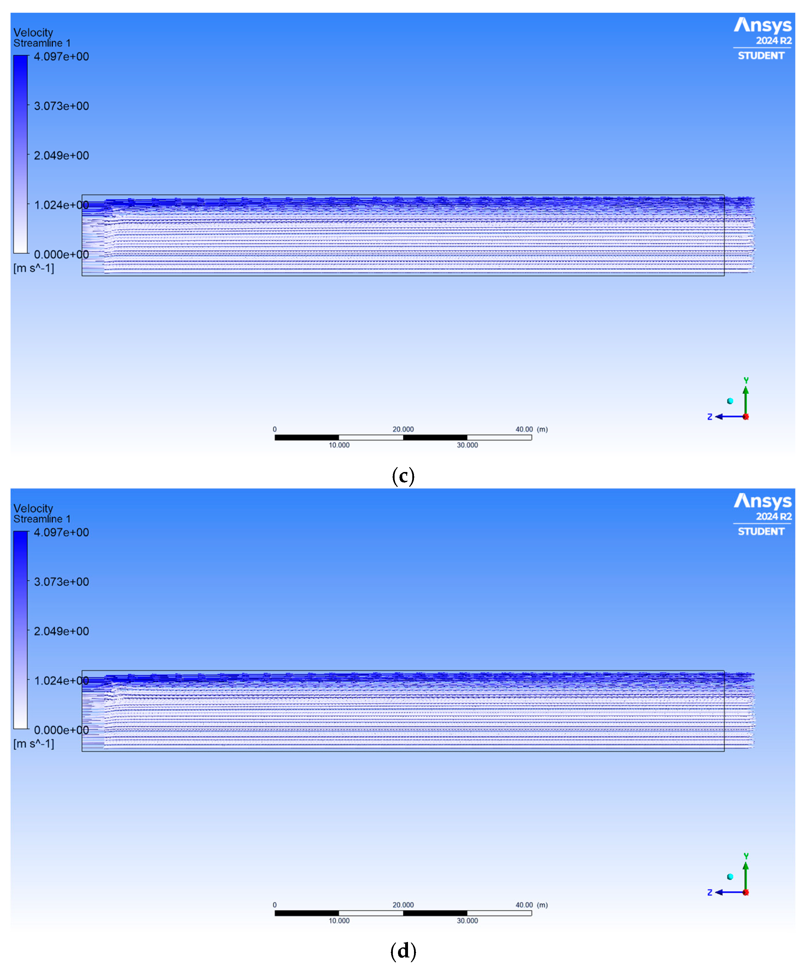
Figure 8.
Water velocity streamlines in Simulation A at different time steps: (a) 0 s, (b) 100 s, (c) 300 s, and (d) 500 s.
Figure 8.
Water velocity streamlines in Simulation A at different time steps: (a) 0 s, (b) 100 s, (c) 300 s, and (d) 500 s.
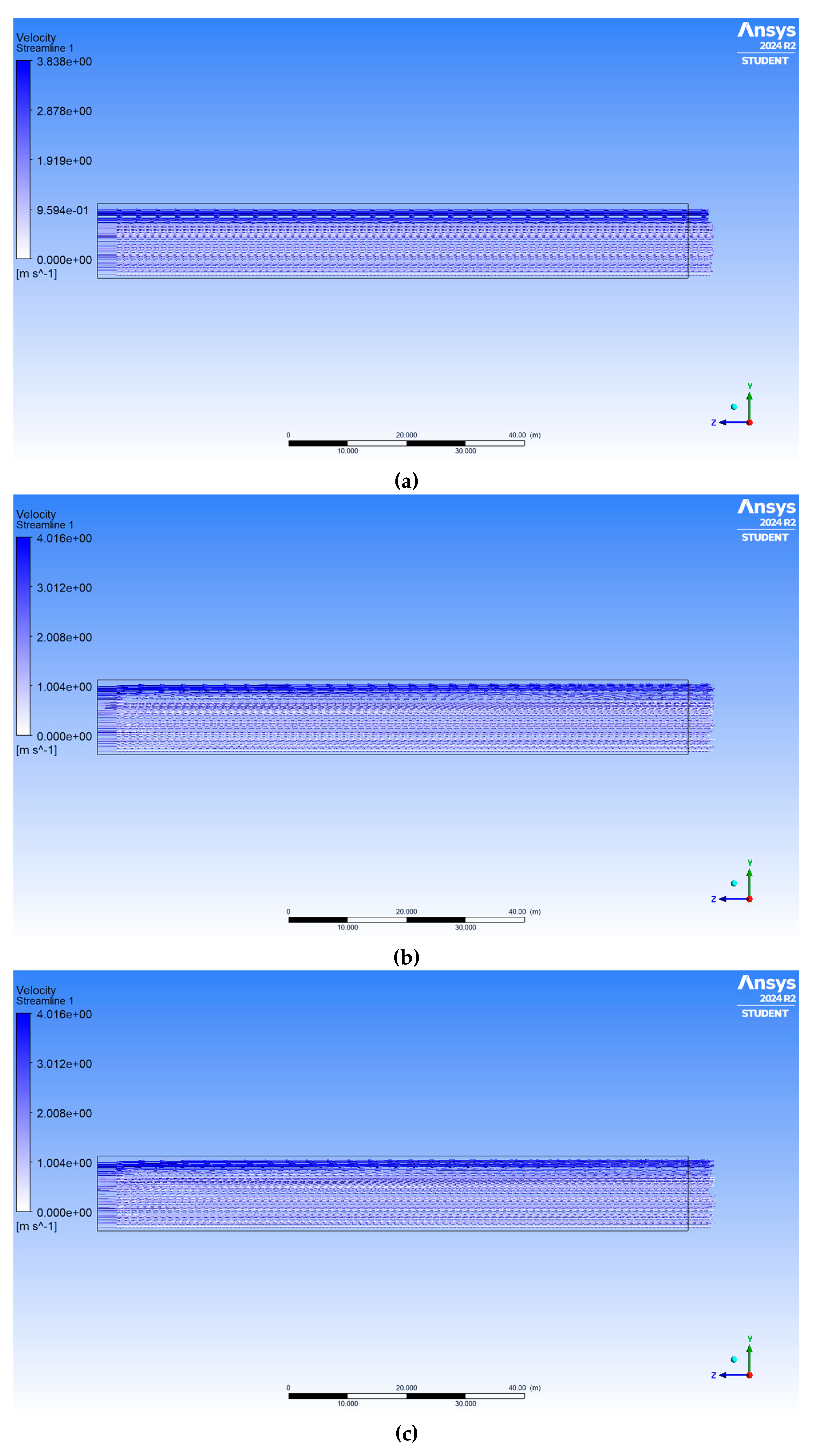
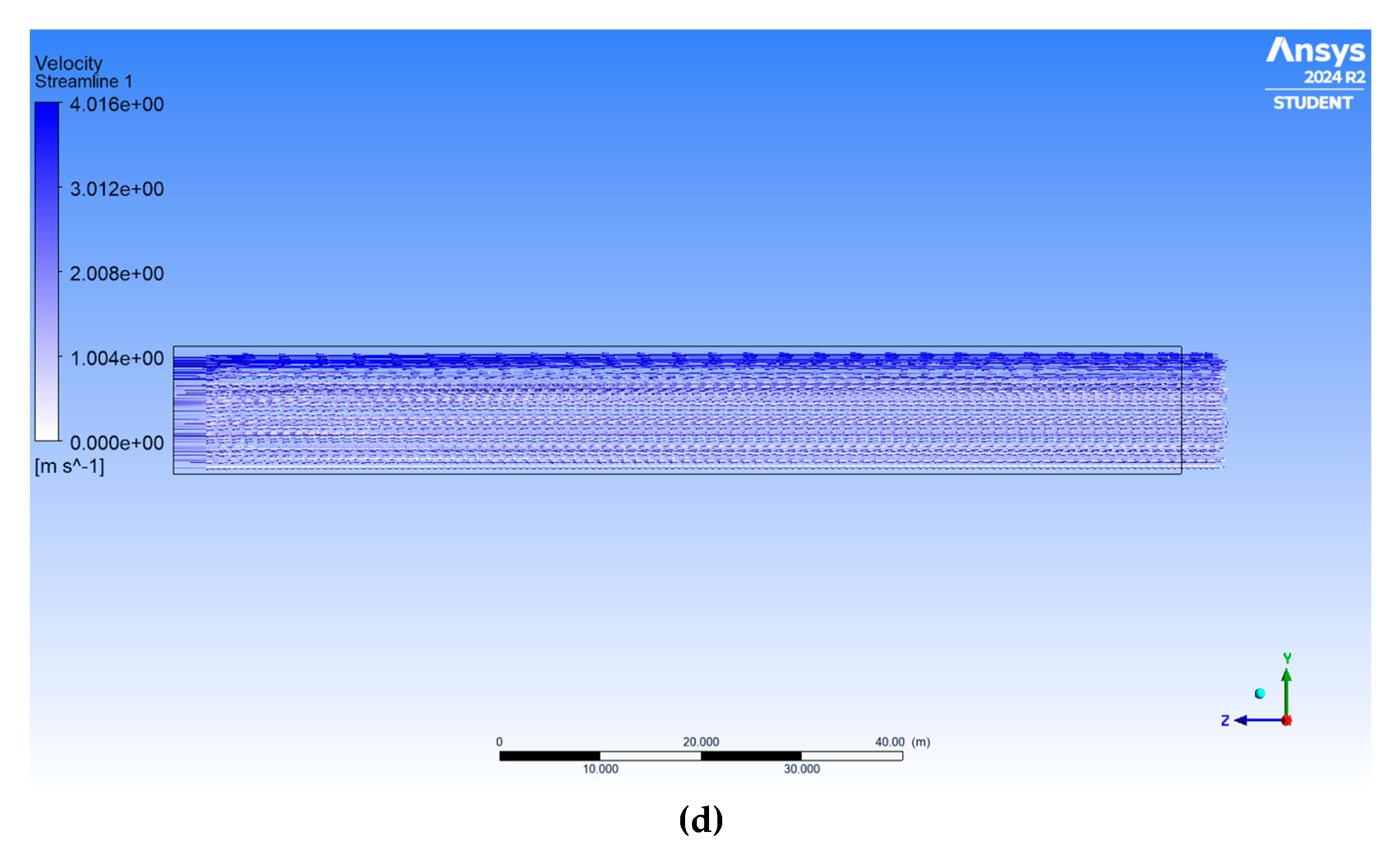
Figure 9.
Density contours at three time intervals: (a) 0 time steps (0 seconds), (b) 600 time steps (300 seconds), and (c) 1000 time steps (500 seconds).
Figure 9.
Density contours at three time intervals: (a) 0 time steps (0 seconds), (b) 600 time steps (300 seconds), and (c) 1000 time steps (500 seconds).
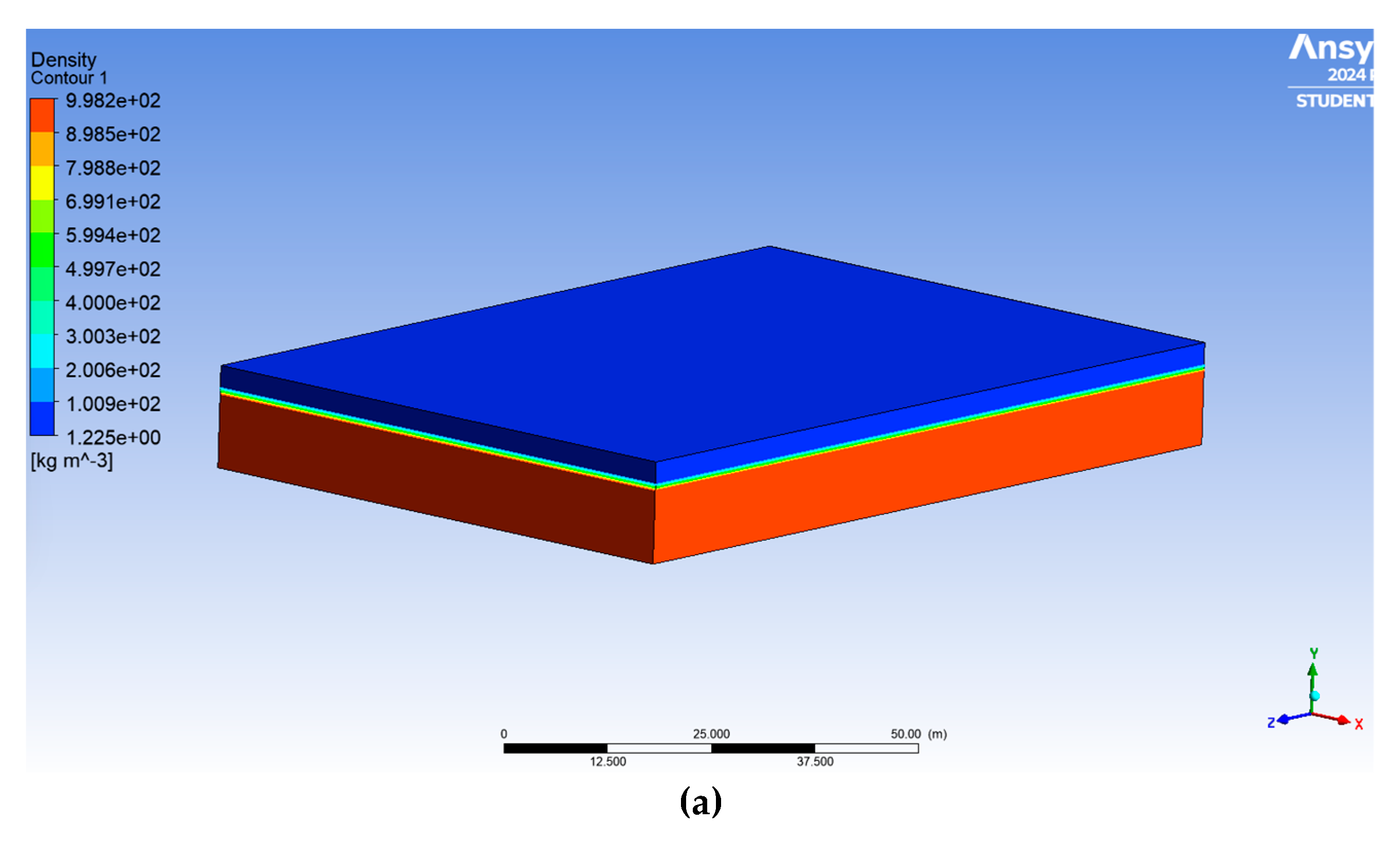
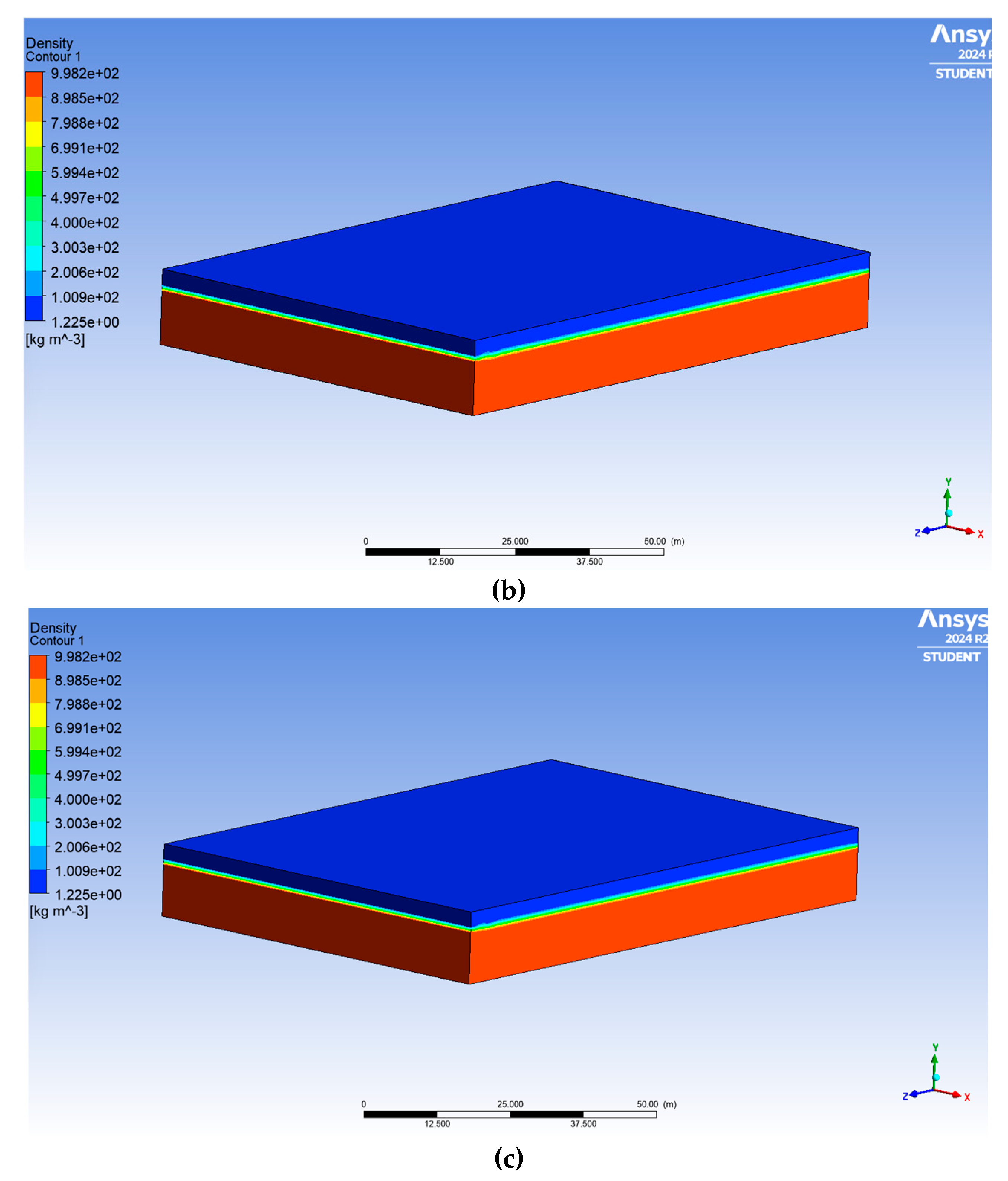
Figure 10.
Pressure contours at three time intervals: (a) 0 time steps (0 seconds), (b) 600 time steps (300 seconds), and (c) 1000 time steps (500 seconds).
Figure 10.
Pressure contours at three time intervals: (a) 0 time steps (0 seconds), (b) 600 time steps (300 seconds), and (c) 1000 time steps (500 seconds).
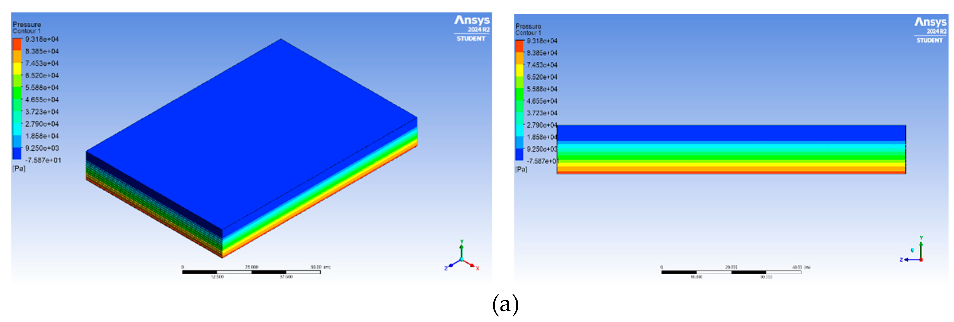
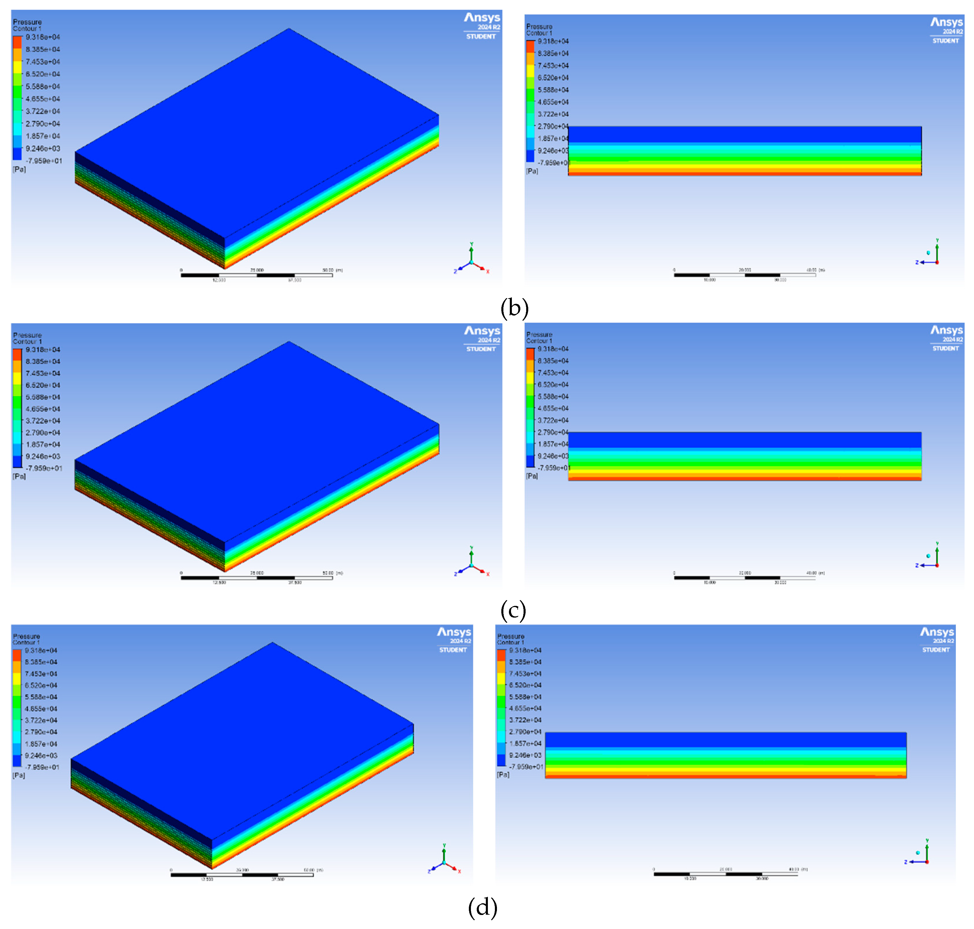
Figure 11.
Air Volume Fraction Isosurface at 500 s.
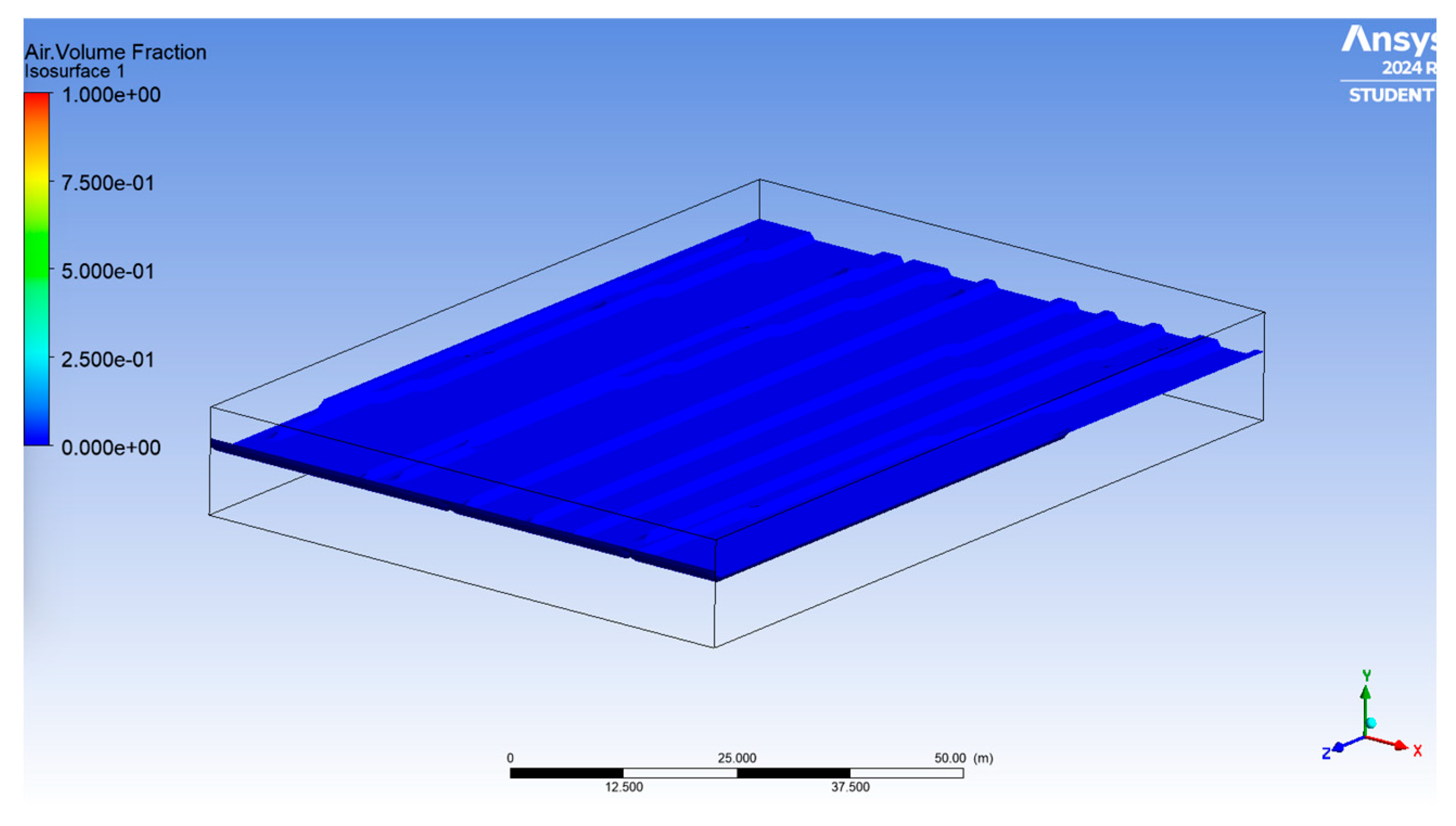
Figure 12.
Traces of PET particles at different time intervals during simulation A: a) 0 s, b) 25 s, c) 50 s, d) 75 s, e) 100 s, f) 125 s, g) 150 s, h) 175 s, i) 425 s, j) 400 s, k) 475 s, l) 500 s.
Figure 12.
Traces of PET particles at different time intervals during simulation A: a) 0 s, b) 25 s, c) 50 s, d) 75 s, e) 100 s, f) 125 s, g) 150 s, h) 175 s, i) 425 s, j) 400 s, k) 475 s, l) 500 s.
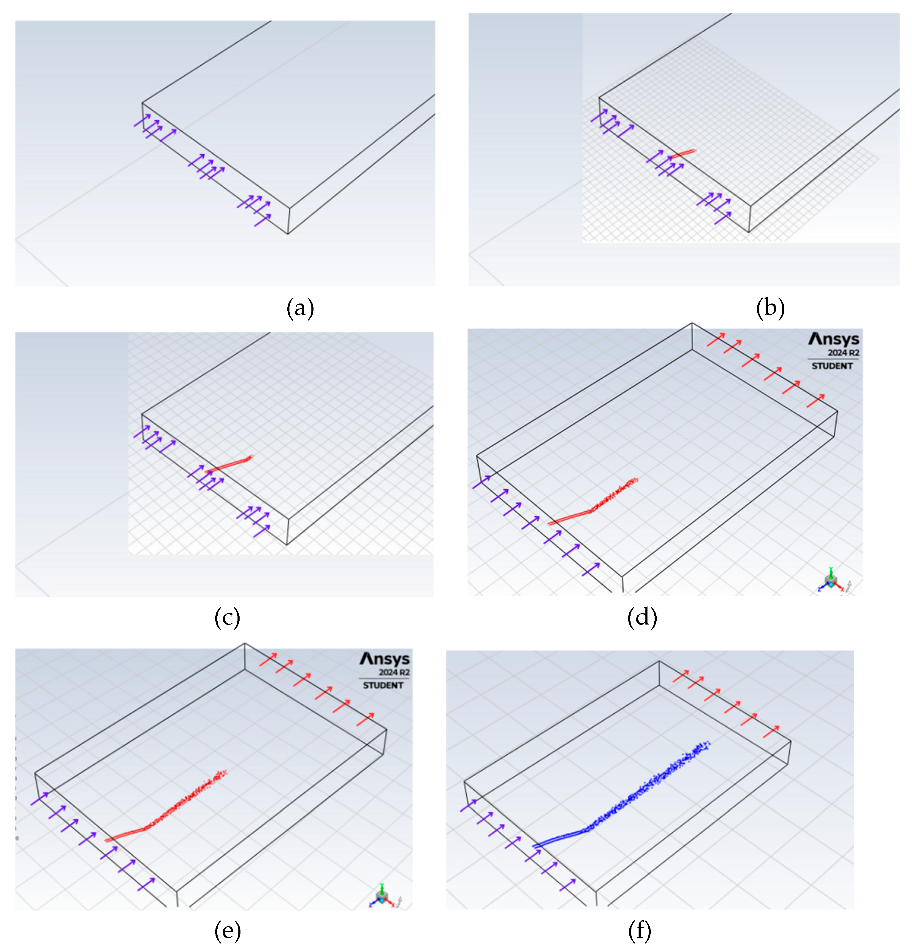
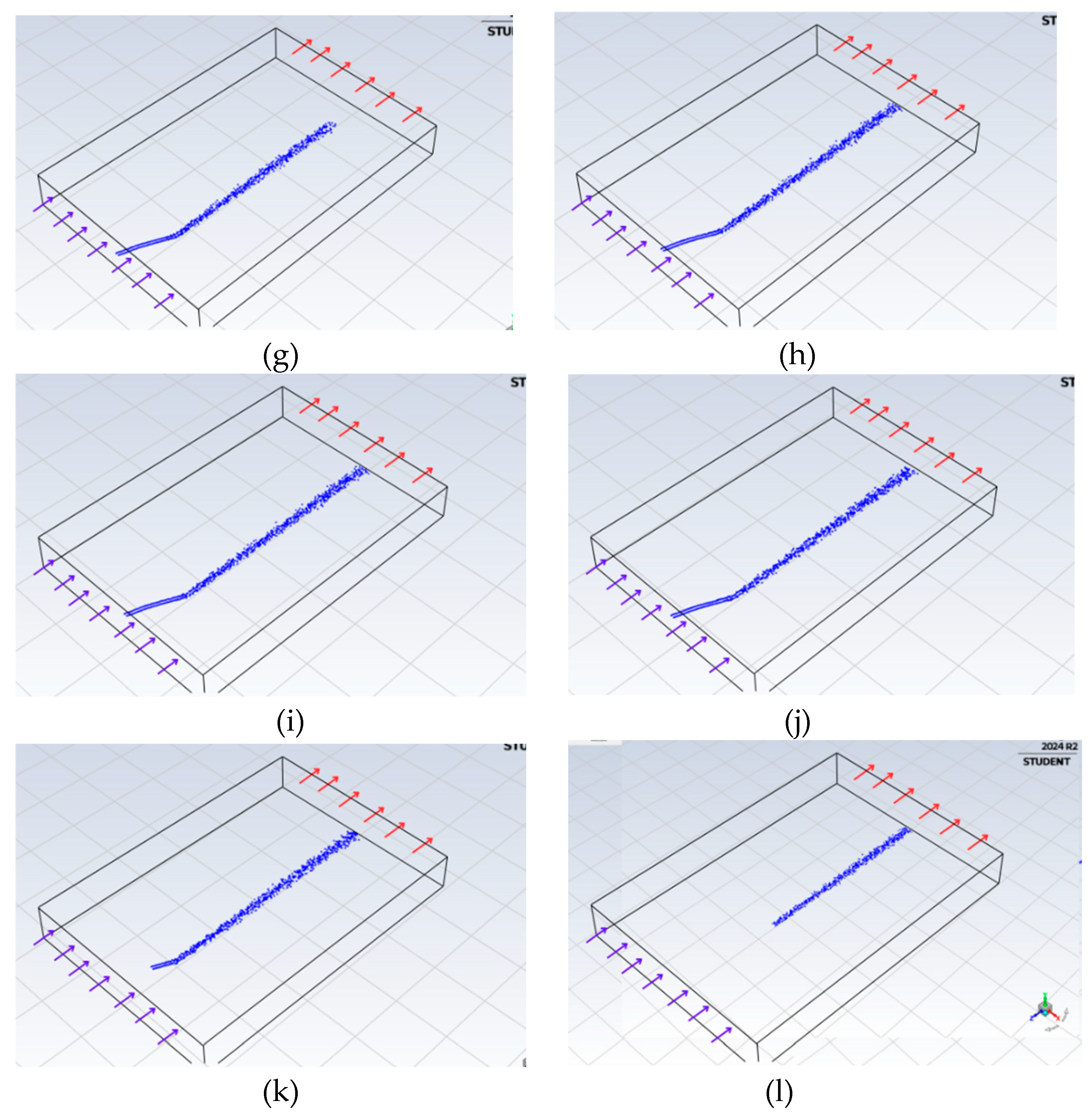
Figure 13.
Particle tracks at 500 s for a water inlet velocity of 0.5 m/s.
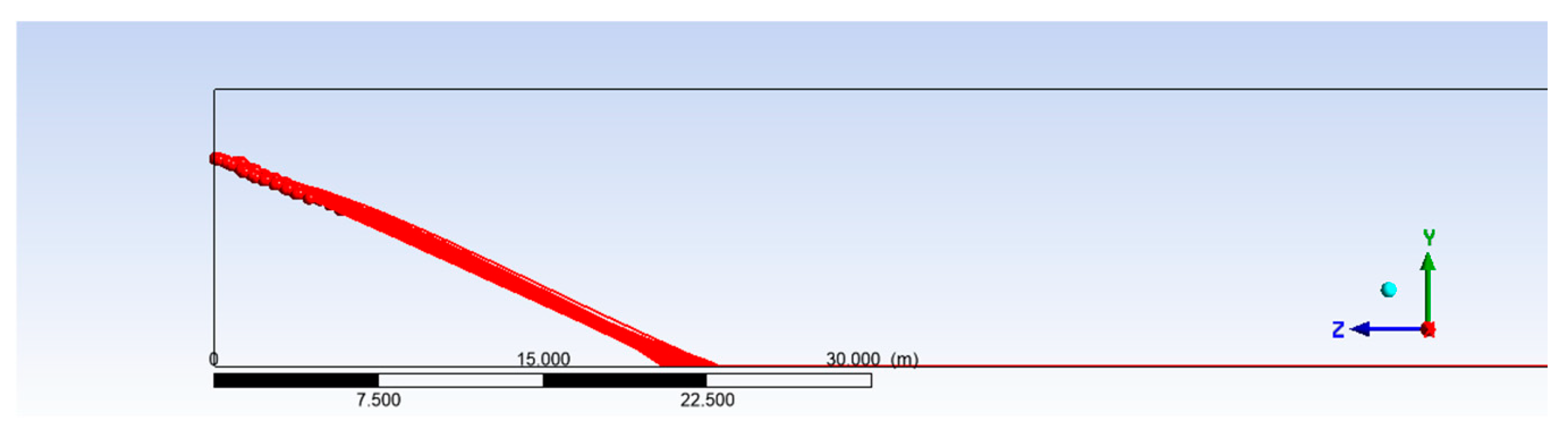
Figure 14.
Traces of PET particles at different time intervals during simulation B: a) 0 s, b) 25 s, c) 50 s, d) 75 s, e) 100 s, f) 125 s, g) 150 s, h) 175 s, i) 425 s, j) 400 s, k) 475 s, l) 500 s.
Figure 14.
Traces of PET particles at different time intervals during simulation B: a) 0 s, b) 25 s, c) 50 s, d) 75 s, e) 100 s, f) 125 s, g) 150 s, h) 175 s, i) 425 s, j) 400 s, k) 475 s, l) 500 s.
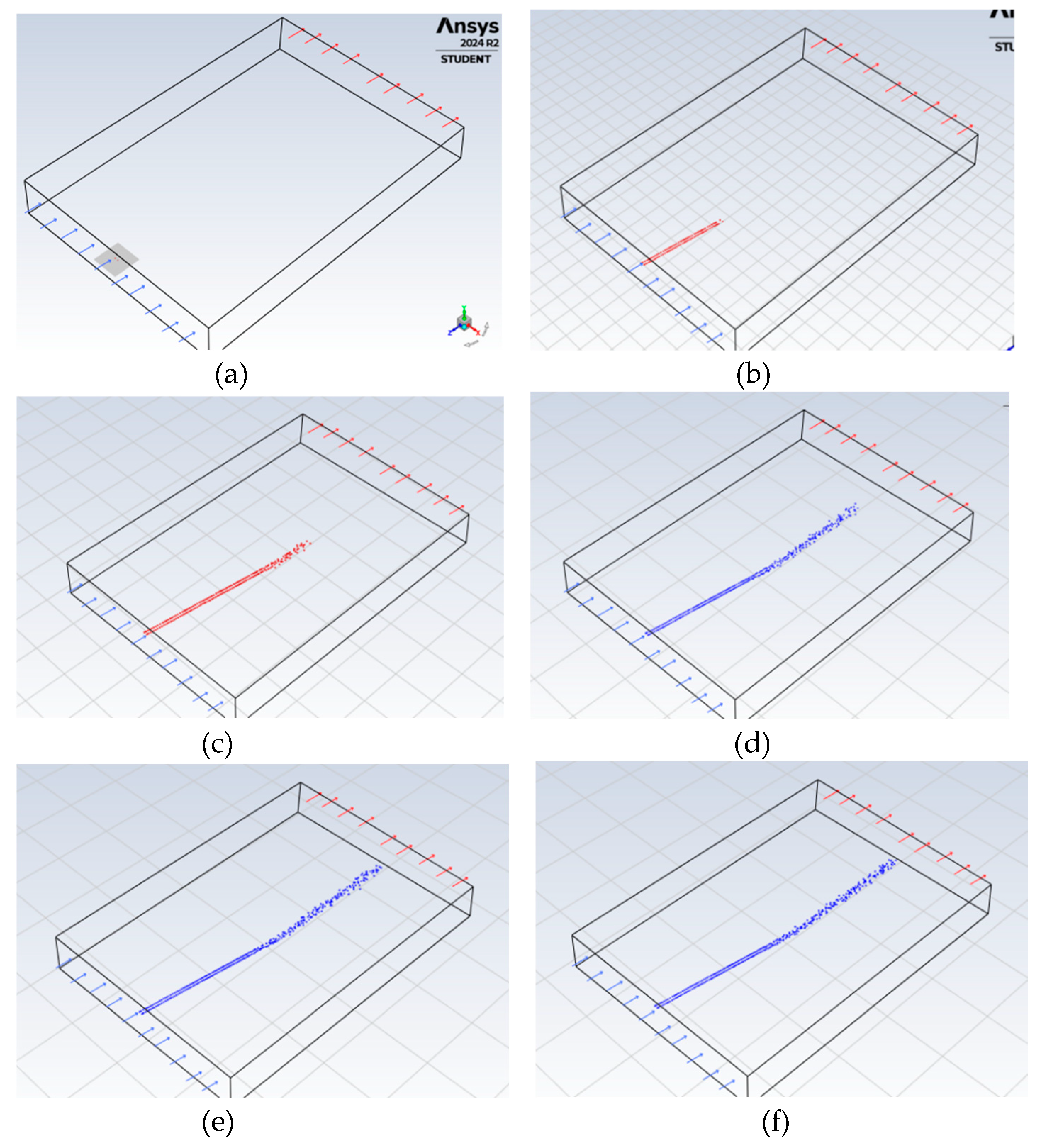
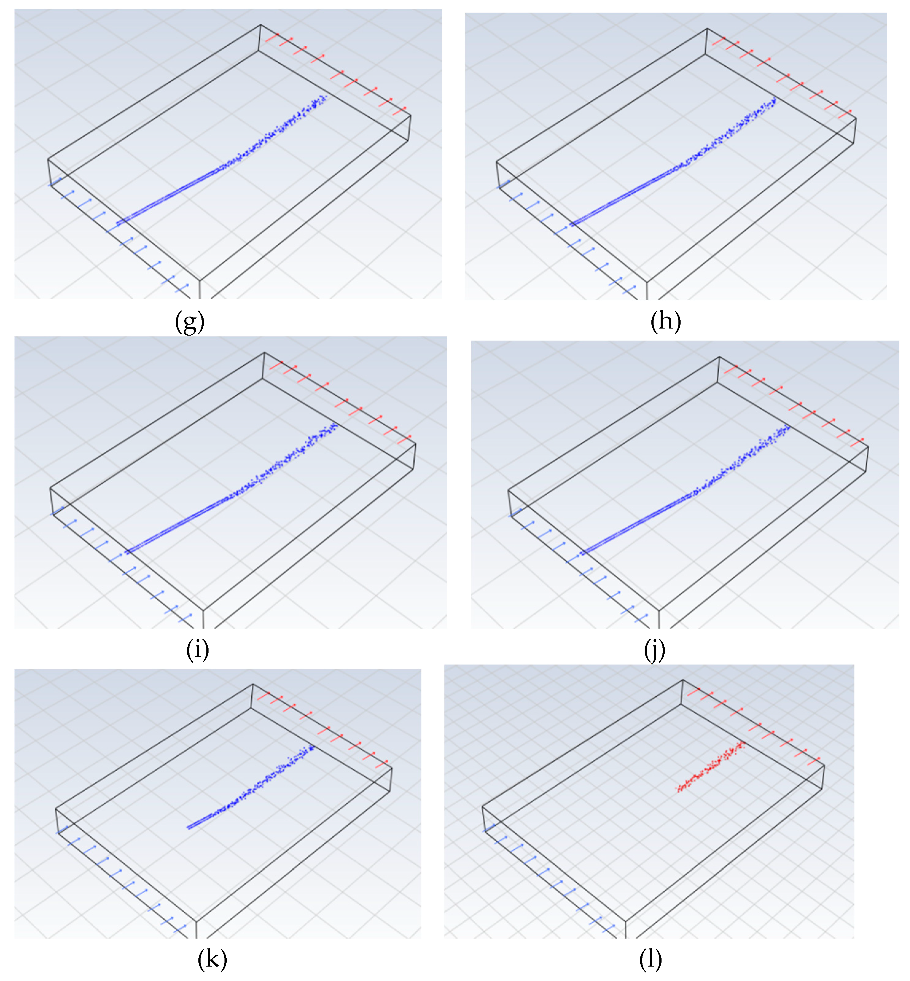
Figure 15.
Particle tracks at 500 s for a water inlet velocity of 1.25 m/s.
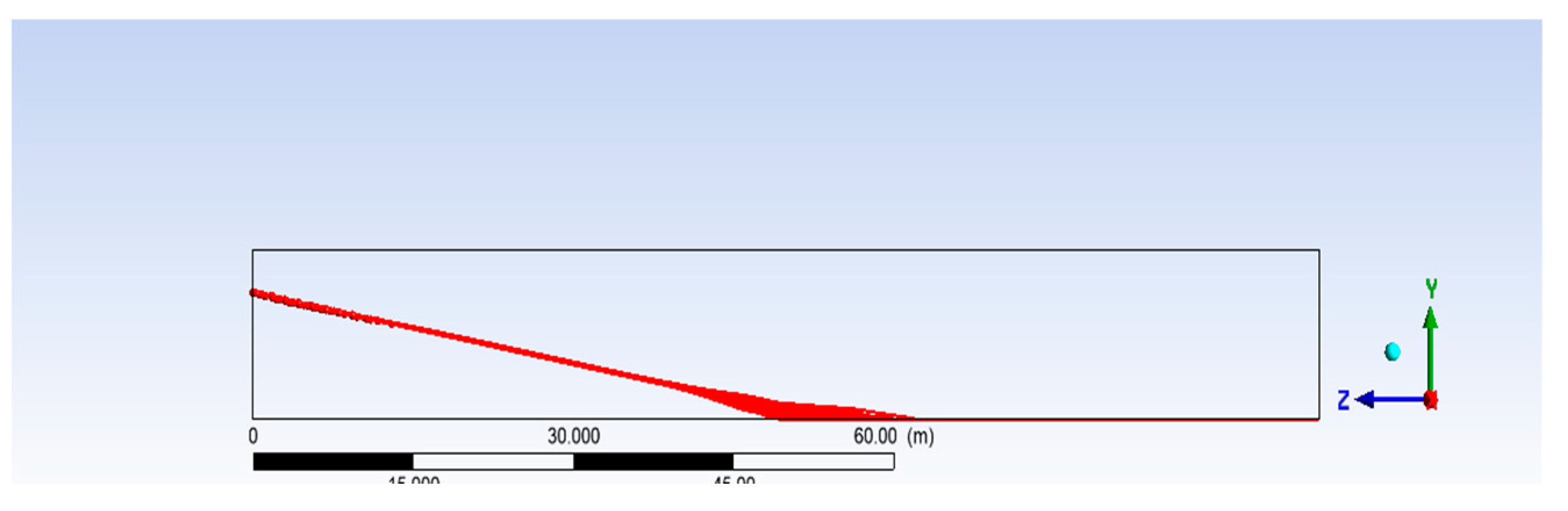
Table 1.
Boundary conditions.
| Type | Description |
| Velocity Inlet | Water and air inlet: water depth of 9.5 m with velocities of 0.25 m/s (Simulation A) and 1.25 m/s (Simulation B), volumetric fraction = 1. Air enters at 3.3 m/s with a height of 3.14 m. |
| Pression Outlet | Water and air outlet, 0 Pa gauge pressure. |
| Wall | No-slip condition applied to the bottom and sidewalls. |
Table 2.
Water velocity at the reference point for different mesh resolutions.
| Parameter | Velocity [m/s] |
| Mesh 1 | 4.270 |
| Mesh 2 | 2.539 |
| Mesh 3 | 2.542 |
| Mesh 4 | 2.177 |
Table 3.
Mesh quality parameters for different mesh resolutions.
| Element Quality | Aspect Ratio | Obliquity | Orthogonal quality | |
|---|---|---|---|---|
| Mesh 1 | 0.65522 | 2.452 | 0.029495 | 0.9973 |
| Mesh 2 | 0.65404 | 2.4633 | 0.018038 | 0.99946 |
| Mesh 3 | 0.66812 | 2.4038 | 0.0013479 | 0.99948 |
| Mesh 4 | 0.66207 | 2.4318 | 0.0063195 | 0.9999 |
Disclaimer/Publisher’s Note: The statements, opinions and data contained in all publications are solely those of the individual author(s) and contributor(s) and not of MDPI and/or the editor(s). MDPI and/or the editor(s) disclaim responsibility for any injury to people or property resulting from any ideas, methods, instructions or products referred to in the content. |
© 2025 by the authors. Licensee MDPI, Basel, Switzerland. This article is an open access article distributed under the terms and conditions of the Creative Commons Attribution (CC BY) license (http://creativecommons.org/licenses/by/4.0/).
Copyright: This open access article is published under a Creative Commons CC BY 4.0 license, which permit the free download, distribution, and reuse, provided that the author and preprint are cited in any reuse.


