Enhancing Fire Alarm Systems with Machine Learning: A Data-Driven Approach to Early Fire Detection

1. Introduction

Fire accidents pose a tremendous risk to human life and property, and delayed detection often leads to disastrous losses. Traditional smoke alarm systems, while being widely used, have some drawbacks, including a high possibility of malfunction. Pincott et al. (2022) stated that smoke alarms may malfunction in approximately 35% of cases, which raises question about their reliability in times of crisis. With advancing technology, employing the use of machine learning for detecting fires presents an exciting solution for improving accuracy and response rates. One of the most tragic recent fire tragedies, the Grenfell Tower fire in June 2017, took the lives of 72 people, with most of the residents reporting that they did not hear any alarms until it was too late (McKenna, 2019). This tragedy underscores the urgency for a more effective fire detection system. Research has shown that the average time taken by people to evacuate in the event of fire is about five minutes [1,2], whereas fires spread within 30 seconds (Scutum, 2024). Therefore, improving the efficiency of fire detection systems is crucial to enable timely evacuations and reduce casualties. This study explores the application of machine learning techniques to enhance the accuracy of fire detection. By analyzing sensor inputs like temperature, humidity, gas release, and air quality, we aim to develop a model that predicts the occurrence of initial fire threats. The research makes use of actual datasets for training and evaluating different machine learning algorithms to ultimately select the optimal method for real-time fire detection. Through this work, we intend to contribute to providing safer environments by coming up with intelligent alarm systems that can effectively counter the dangers of late fire alarms [3,4,5].

1.1. Dataset description

Before going into training the model, it is vital to understand the dataset first in order to know what tools one can work with. Overall, the dataset has a total of 16 well-put columns. Some of which will be explained thoroughly below.

1.2. Characteristics and Source Index

This variable is premade for more efficient use of the dataset. It enables easier data retrieval and simplifies operations. As each row represents an instance of extracting data, it helps identify all the variables that took place at the same time. This variable is not extracted from a source but rather assigned and incremented to locate other variables more easily. Since the creators of the dataset only used it as an index, there is no name to define it, and it shows up as “Unnamed: 0” once extracted to a dataset environment. This can be simply mitigated with a renaming of the column.

1.3. UTC

This variable is for tracking the time a fire was detected. It is measured in Unix time which is not readable for humans directly. For example, “1654733331” would be equivalent to June 9, 2022, 09:28:51. This type of Unix time is highly compatible with a large number of languages and makes it simple for the dataset to store the value as it is one continuous number instead of several long numbers and alphabets. It also provides more consistent time reference across multiple sources from different countries as it is taken based off the universal time constant with no specified time zone. Some fire alarms possess an internal time clock that may measure this constantly whenever a fire is triggered and relay the information directly to the system [6,7].

1.4. Temperature

While not the only important column, temperature is one of the key data to extract as differences in temperatures are strongly associated with the occurrences of fire. To make sure the dataset is easily extensible, this column is measured in a global standard of Celsius. Most temperatures fall around 20-22 °C which indicates a normal and safe value for most situations, although this may not always be the case. It is worth noting that in this column, the temperature’s speed of fluctuations is more important than reaching a specific value as a fire in a cold environment may fail to reach a temperature high enough to alert the detector. This column would be extracted through thermometers converting the readings to electric signals to feedback the system [7,8].

1.5. Humidity

This shows the overall water content present in the air. While lower humidity may be associated with fires drying out the air, it is important for the detector to monitor this as high humidity may also cause false alarms. As there is more water content in the air, it becomes harder for the system to detect small organic particles indicating a combustion taking place. By accounting for the water vapor, the sensor can easily adjust its sensitivity and readings of variables. Sensors such as DHT11 or SHT31 are capable of integrating with a fire detector and extracting this variable [9].

1.6. TVOC

Total volatile compound. Rated in parts per billion (ppb) which provides more precision in detection. It measures the amount of organic chemicals that can become highly vaporized. They are emitted from everyday materials such as cleaning supplies, paints, hygiene products… etc. These are highly flammable and may cause a higher risk of fire so detecting them earlier may set the stage for other variables and boost the accuracy of readings. They don’t only indicate the potential of a fire but also when it is currently happening as they are released after objects become burned. They’re extracted from sensors such as a MOX (metal oxide) detector [10].

1.7. 2eCO2

Measures the equivalent amount of co2 in the air, similarly in parts per billion (ppb). This variable can pick up the effects of a fire prior to the expulsion of smoke and flames, providing earlier detection and more variation on the diversity of constants which potentially boosts accuracy. Sensors may use infrared light to measure co2 levels as the gas absorbs a specific level of light or by using electrochemical sensors to measure the change in conductivity from the reaction of co2 with chemical compounds [11].

1.8. Raw H2

Hydrogen is one of the most flammable elements and the fact that it is extremely common makes it a prime candidate for observation. With a high sensitivity to ignition of up to 75% (AICHE), it may easily cause a violent explosion. It is considered odourless and disperses rapidly through the air which makes it hard to detect by manual vision. Similar to eCO2, it is detected through electrochemical sensors and infrared sensors.

1.9. Raw ethanol

The same goes for ethanol, while not as common, it is still used in daily products such as hygiene products that may pose risk greatly needed to account for. It has greater value if the fire detector is installed inside industries with more common uses for it such as distilleries. Ethanol is mainly detected through sensors such as forensic alcohol gas detectors.

1.10. Pressure

The overall pressure of the air should also be considered as it plays a major role. As a fire is ignited, the air pressure rises as the air begins to swell. This is speculated to be even faster than small particle detection as the swelling of air is faster in terms of change. Not to mention, based on pressure, fires can behave extremely differently and may cause more fatal consequences. This can be sourced from pressure sensors or air sampling systems that measure the rate of change in pressure between two prior and current instances [11].

1.11. PM 1 and PM 2

This denotes the particle matter (PM) after combustion. This can help in detecting a false alarm from a real one. While still being the aftermath of a fire, these can be detected before larger particles of smoke reach the alarm. Allows for more efficiency regarding time management and early detection. It can be extracted through sensors with light emission that analyzes how particles are hit by the light.

1.12. NC 0.5 | NC 1 | NC 2.5

The number concentration of particles with different diameters of 0.5, 1, and 2.5 respectively. Unlike PM that counts the number of particles in the air, NC measures the overall weight of these particles. This weight can greatly help with understanding the type of smoke and knowing whether it is dangerous and should sound an alarm and when it is a safe kind of gas. It is extracted from air sampling through a series of filters and each particle is weighed for its mass [12].

1.13. Fire Alarm

This acts as a simple Boolean representing whether a fire alarm was set off. It is sourced from the fire detector itself and stored in the dataset system to help know and review when it was set off for accurate training [13].

1.14. High-Level Statistics

In order to better describe and gain a deeper understanding of the data, functions such as data.describe() were used to analyze high level statistics. By starting off with data.head(), we can inspect the dataset’s first few rows and check for any kind of errors. The dataset looks clean and fully documented from the initial findings according to the output. The next step would be to understand each feature’s descriptive statistics. It is worth noting that the dataset has only been analyzed in the most important and relevant columns to our research [14,15].

Figure 1. Temperature Statistics.

Figure 1. Temperature Statistics.

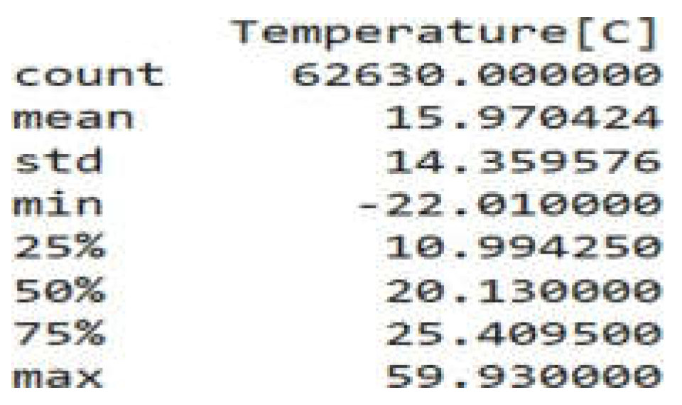
According to the figure above, temperature is shown to have a count of 62630 entries which matches the dataset rows and shows that there are no missing values left out. The mean is 15.97, which shows the average temperature taken by the alarms. While normal room temperature usually falls around 20-22 degrees, a mean of 15.97 in the dataset shows that there may have been many instances of colder temperatures to drive the value down which could be the standard deviation is around 14.35 from the mean which indicates temperature is mostly ranging commonly around 30 to 1.62 degrees. With a minimum of -22 degrees and a max of 59.93, temperature is shown to have a diverse range of environments that exceeds the standard deviation by a large percentage. The theory of colder temperatures bringing the mean down is made clear by the 25^th and 50^th percentile that denote at least half of the dataset falls below average temperatures while only the 75^th percentile reaches a measly 25.4 degrees. The data may be skewed towards lower values [16,17].

The count shows no missing values for this column either. While most buildings have an average humidity of 40-45%, the dataset shows a somewhat of a similar value with an average mean of 48.53% humidity. The standard deviation is a small 8.86 which indicates most values have been of an average humidity level. The 25^th percentile shows a quarter of data was under 47.53 with 75% being under 53, this supports the idea of a small standard deviation as most instances have been around the mean. However, with a minimum of 10 and max of 75, this may just indicate the presence of outliers as the extreme values are far from the average deviation of a mere 8.86 [18].

With no missing rows, this shows the average concentration of TVOC to be around 1942 with a standard deviation of 7811. Since the minimum is 0 and deviates by only 1942, this means the standard deviation may have been influenced by higher, more extreme values. The values show that 75% of the data fall below 1189, which is lower than the mean by a few digits. While most values are leaning towards a lower amount, this shows the remaining values above 75% are extremely high. This is reinforced by the max value of 60000 which deviates from the mean at a critical sum of 58,058. While this may indicate the presence of outliers, this may also have real life implications of actual fires, when a lower amount of tvoc may be more common but once released it might be in gigantic numbers.

This column is a similar example, although clearer. The mean of 670 may not entirely reflect the median as there is a clear sign of extreme values skewing in a higher direction. As the 25^th till 75^th percentile shows values well-knit around 400-438, a higher mean indicates it is being pulled by extreme values, as shown in the max of 60000, this is skewing results [18,19,20].

This column is very stable. With a mean of 938 and standard deviation of 1, almost all descriptions are similar which shows that most common values are centered around 938. It is a good thing that there are no outliers. However, this lack of deviation shows that the alarm may work at a high sensitivity to pick up the smallest changes in pressure while not needing drastic amounts of fluctuations. While 75% of data falls below 2.24, this indicates that it is more common to have lower values of this data while still having extreme values of 51914 as a max. It is unlikely for the max values to be outliers and may indicate that, much like CO2 and TVOC, it may be low values until a large release upon triggering. This column looks standard with minimal outliers. The average of 12942 with a deviation of 272 is shown in the percentiles. However, the minimum of 10668 may be considered an outlier as it deviates by more t272. This column is simple and straightforward. Since this is a binary value of a Boolean indicating whether there was a fire alarm sounded or not, the only important statistic to pick up is the mean. By measuring the mean, one can tell that there have been approximately 71% of cases where the alarm was sounded [21].

2. Research Methodology

This study aims to develop an accurate and reliable fire detection system based on machine learning algorithms. It includes some crucial stages like data collection, preprocessing, feature selection, model training, evaluation, and validation. The stages are all focused on making the proposed fire detection model credible and strong [22,23,24].

2.1. Data Acquisition

The data for this study is from Kaggle and is sensor data for fire occurrence. The dataset contains 16 significant features, which are temperature, humidity, gas, pressure, and particulate matter. The dataset is set to accommodate real-time fire risk data.

2.2. Data Preprocessing

To make the dataset suitable for machine learning [25,26], the following preprocessing is carried out:

• Handling Missing Values

Since there are no missing values in the data, imputation is not required. Data integrity is checked for completeness, however.

Removing Unnecessary Columns: Predictor features that are less important to predict fires (e.g., timestamps and redundant high-correlation features) are removed to reduce the complexity of the model and prevent overfitting.

Outlier Detection and Treatment: Z-score and Winsorisation techniques are applied to treat extreme values while preserving meaningful variations in the data.

Feature Scaling: Standardization is accomplished using the Standard Scaler method to normalize feature values and improve model performance.

3. Exploratory Data Analysis (EDA)

EDA is done to understand the relationships between different variables and recognize patterns accountable for fire dangers. Key methods are:

Correlation Analysis: Heatmap is used to identify highly correlated features and eliminate redundant variables [27].

Scatter Plots and Pair Plots: Visualizations highlight potential feature relationships that are important for fire detection.

Histograms and Density Plots: These are utilized to assess the distribution of data and identify skewness or anomalies.

4. Machine Learning Model Selection and Training

Three supervised learning models are selected for comparison:

Decision Tree Classifier: Included due to its interpretability and ability to handle non-linear relationships.

Logistic Regression: Chosen for its efficiency in binary classification and lower computational complexity [28].

Random Forest Classifier: Employed as an ensemble learning technique to improve accuracy and generalization. The data is split into training (70%) and testing (30%) sets for the evaluation of the model's performance.

5. Model Evaluation and Validation

For the evaluation of the model's performance, the following metrics are used:

Accuracy: Measures overall correctness of prediction.

Precision, Recall, and F1-Score: Measures the trade-off between false positives and false negatives.

Confusion Matrix: Shows classification performance with correct and wrongly classified examples.

Cross-Validation: 5-fold cross-validation is utilized to ensure the model generalizes well to unseen data.

6. Model Optimization and Selection

The most promising model is shortlisted based on the evaluation metric. Hyperparameter tuning is carried out to optimize the chosen model for enhanced efficiency. The optimized model is then evaluated on an independent data set to validate its reliability for real-world fire detection applications. With this step-by-step methodology, the study aims to develop a successful machine learning-based fire detection system that ensures safety by reducing false alarms and increasing early detection of hazards.

7. Correlation Analysis

Correlation analysis is crucial in feature engineering and feature selection since it informs us on finding the interactions between features and their impact on the target variable. The correlation matrix was used in the creation of a visual heatmap of the correlation coefficient between all pairs of features, and the coefficients varied between -1 (strongly negative) and 1 (Strong positive correlation). After visualizing the heatmap the high correlation factors can be redundant and must be removed to prevent multicollinearity and overfitting that can lead to biased predicted by the model since they can the stronger correlation are assigned the higher priority in model training.

Figure 2. Correlation Matrice Output.

Figure 2. Correlation Matrice Output.

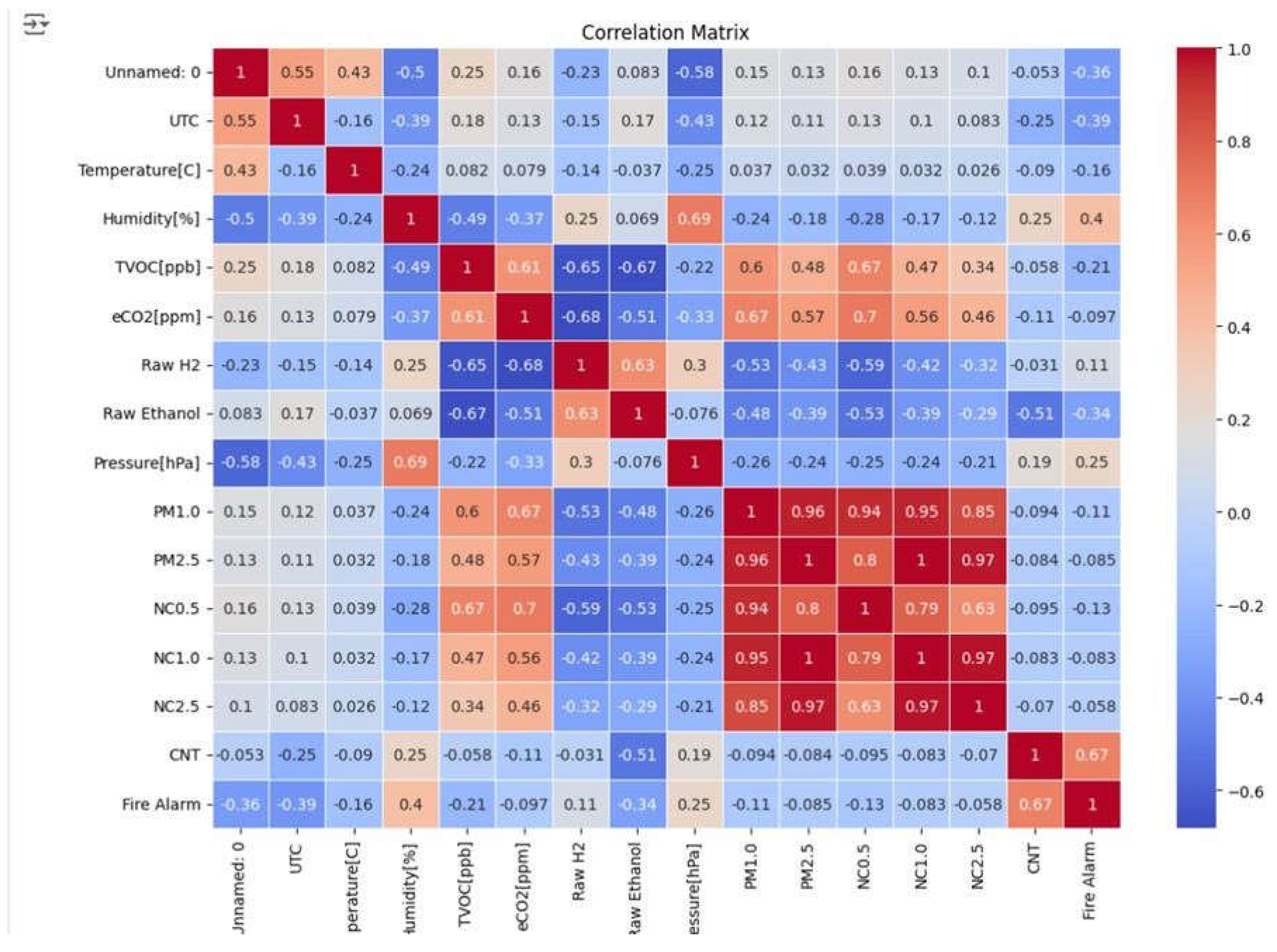
Removing Unnecessary Columns:

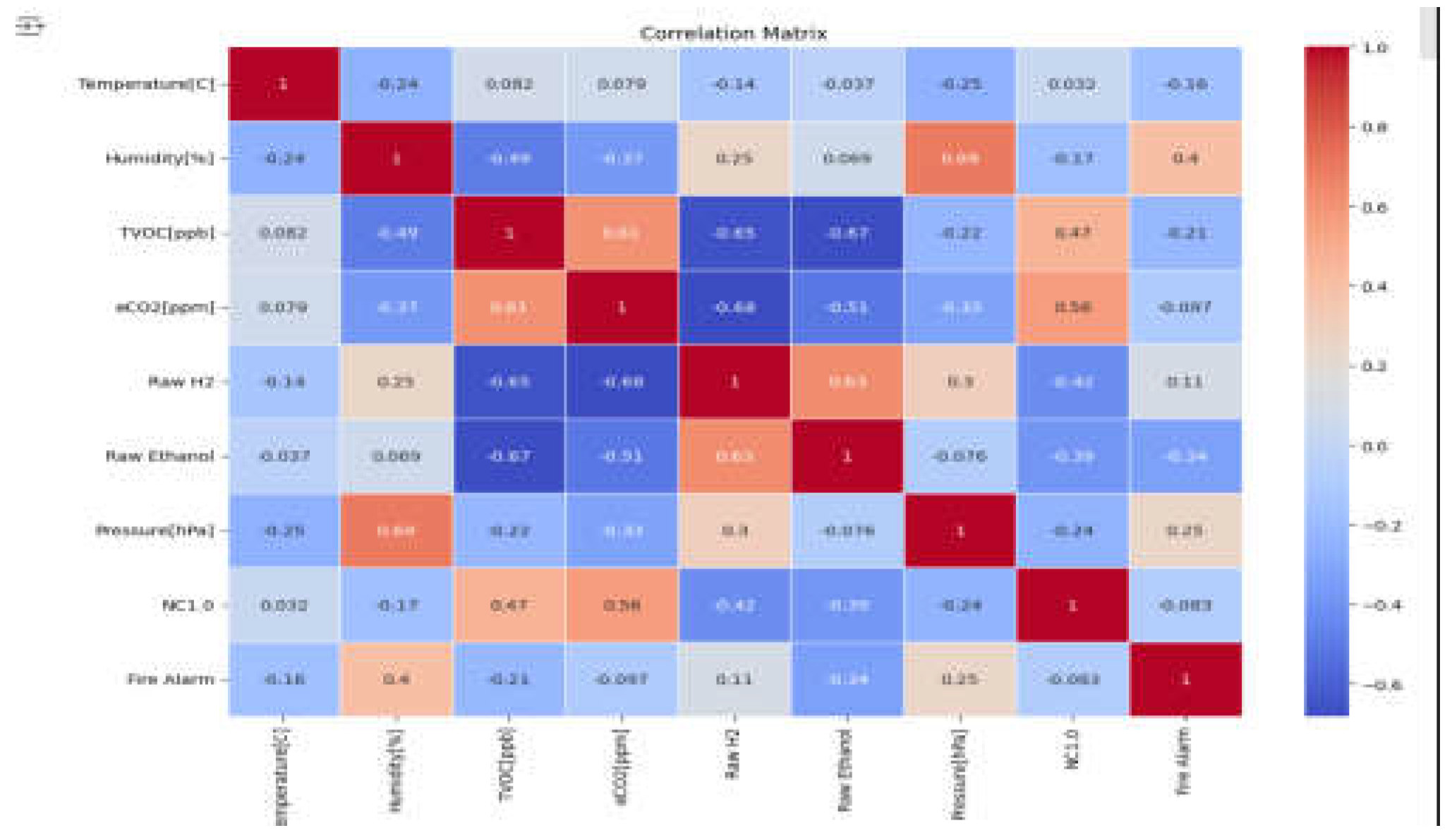
These columns have been taken out for their irrelevance for example unnamed is a counter that will not assist the model, and UTC is the time data collected it will only affect the model in a negative way. PM 1.0, PM2.5, NC0.5, NC1.0 NC, 2.5 in the correlation matrix all contained very high correlation coefficients, so all of them were equally contributing so to avoid redundancy we deleted all and kept NC1.0. These columns have been dropped to avoid overfitting and improve model efficiency and prevent multicollinearity. Then after deleting the columns the new correlation matrix is presented. There are two low correlation values that are still in the model but weakly helping somehow were kept as there are not many columns so their negative effect would be close to zero.

Figure 3. Correlation Matrix.

Figure 3. Correlation Matrix.

Data Splitting 

To check if a machine learning algorithm generalizes well on unseen data so it needs to be split onto 2 subsets training and testing subsets. In the above code the test size was 0.3 showing 30% of the dataset was allocated to the testing subset and 70% training subset.

Feature Scaling 

Machine learning algorithms like logistics regression are sensitive to the magnitude of the input data since features with large values have the capability to overshadow features with small outcomes resulting in unstable and biased outcomes. The scaler.fit_transform was utilized to compute the scaling parameters with respect to data given and afterward after the establishment of parameters via the training dataset scaler.transform was utilized to achieve the same conversion on the test subset without the use of fresh scaling parameters. This method has the advantage of scaling the dataset consistently and keeping the model in its originality during training and testing of it.

Treating Outliers: 

Use tools such as Z-scores in order to identify rows of outlier values and subsequently they would be addressed through winsorize the values and establishing a specified threshold = 3 sets the outlier threshold. Any value with a higher or lower Z-score than 3 is designated as an outlier. outliers = (z_scores.abs() > threshold).any(axis = 1) picks rows that have at least one feature having a Z-score more than the threshold.abs() function for treating both negative and positive outliers and.any(axis = 1) whether any column surpasses the threshold. Then we form a new dataset to winsorize the outliers without modifying the original dataset then using mean and standard deviation we can calculate the lower bound and upper bounds of each feature to identify the outliers and then we winsorize their values. Lastly, the data is graphically represented for comparison before and after winsorizing by applying visualization methods.

Figure 4. Histogram output before and after winsorization for Temperature and humidity.

Figure 4. Histogram output before and after winsorization for Temperature and humidity.

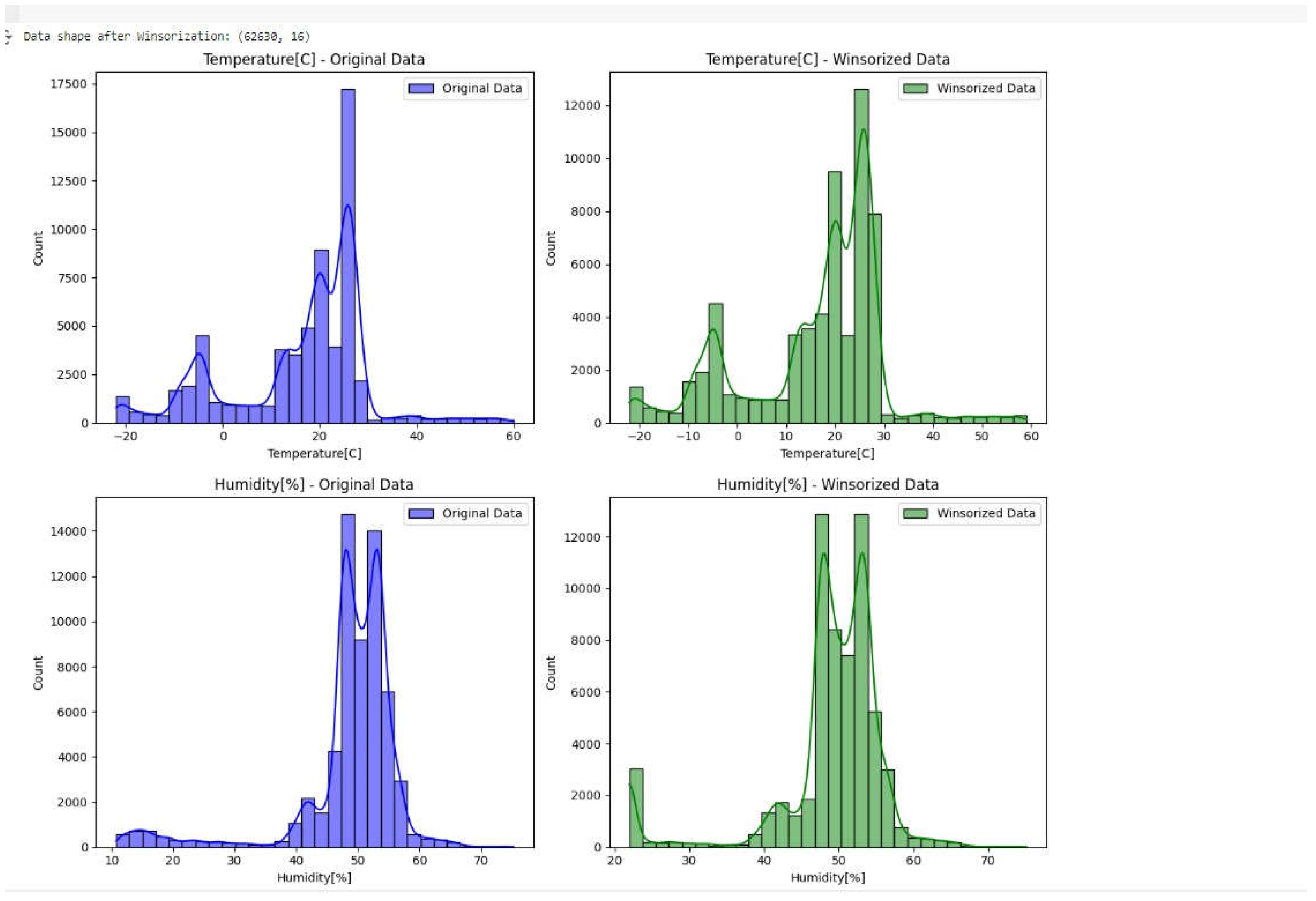
Figure 5. Histogram output before and after winsorization for TVOC and eCO2.

Figure 5. Histogram output before and after winsorization for TVOC and eCO2.

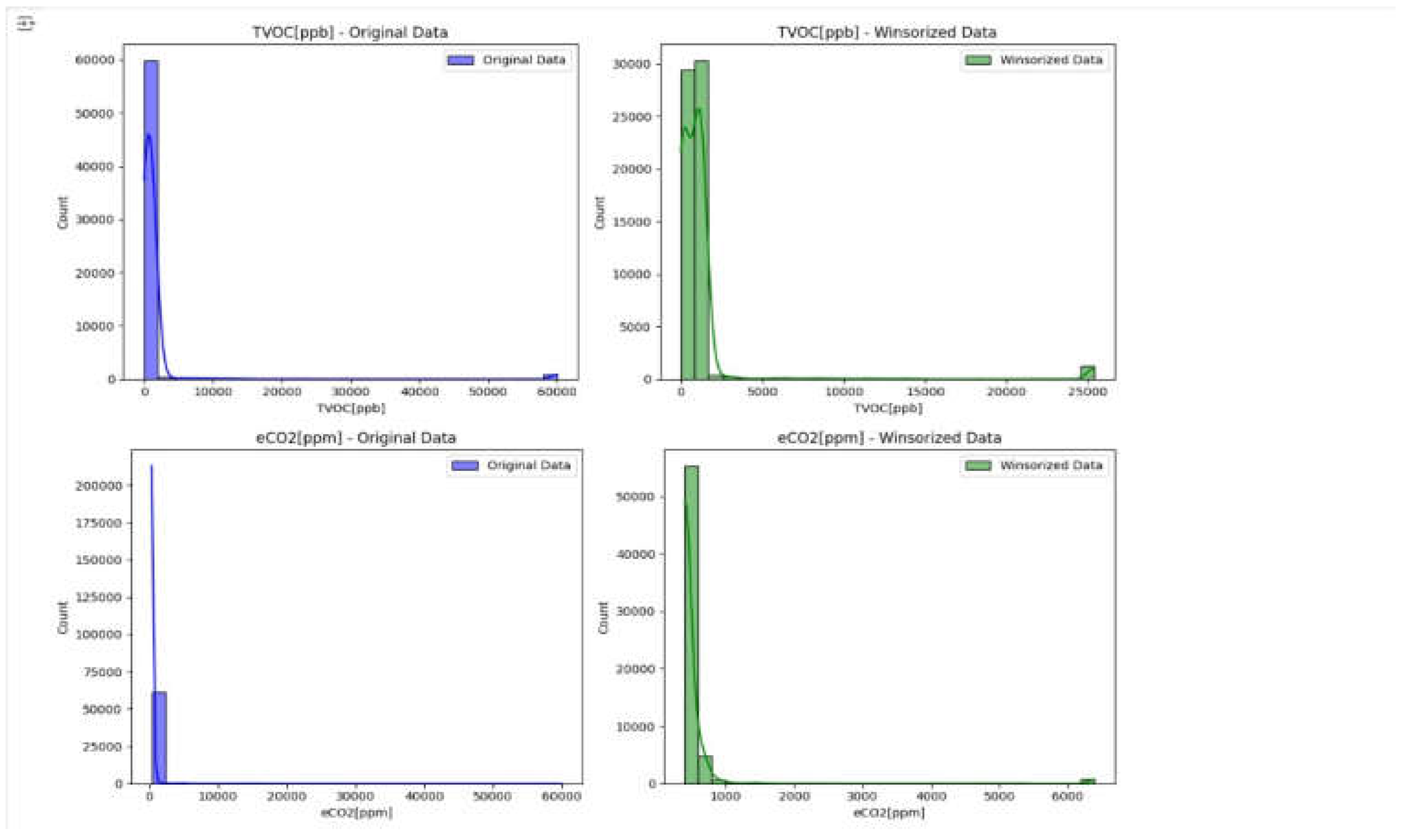
Figure 6. Histogram output before and after winsorization for H2 and ethanol.

Figure 6. Histogram output before and after winsorization for H2 and ethanol.

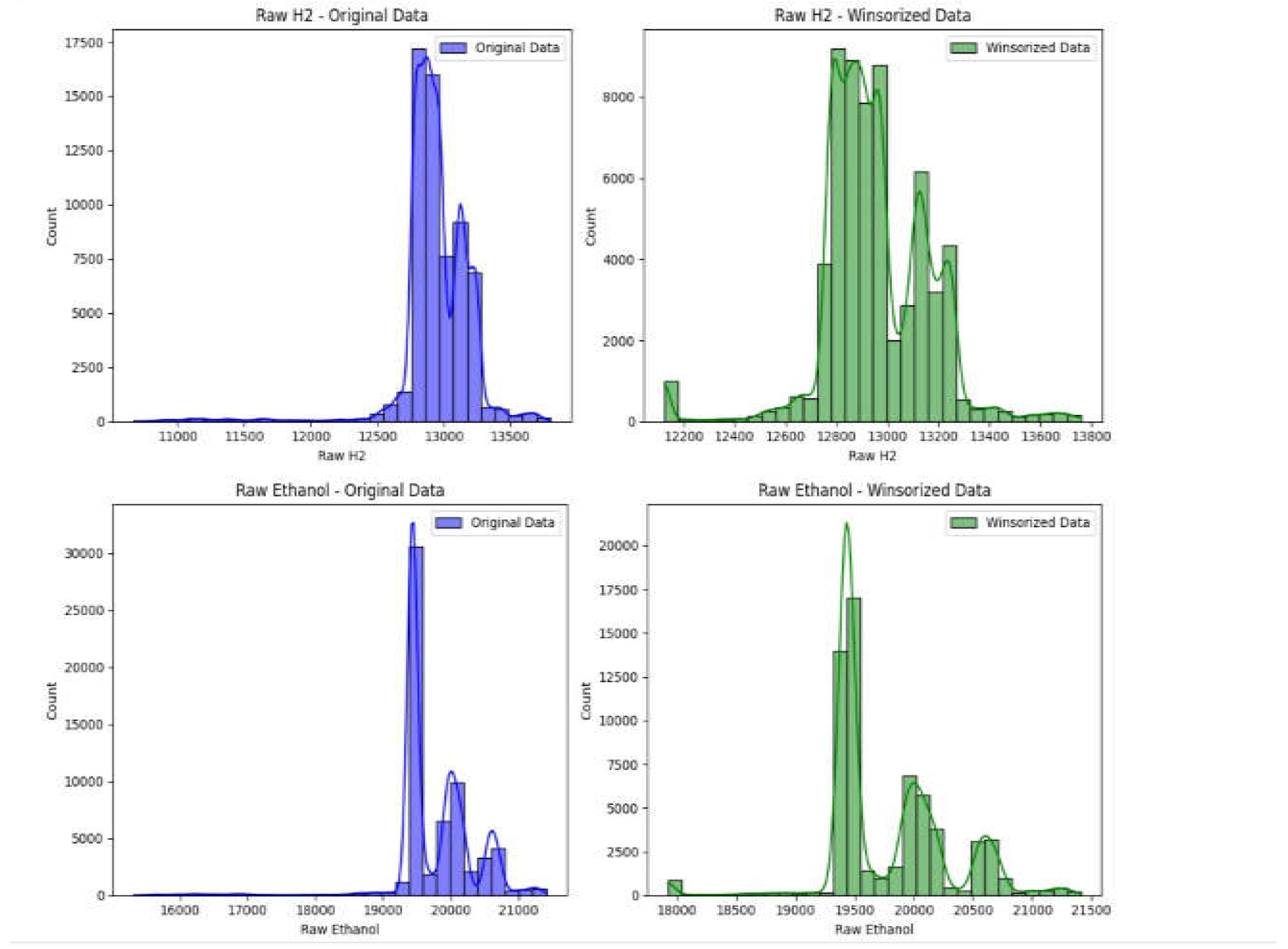
Figure 7. Histogram output before and after winsorization for Pressure and NC1.0.

Figure 7. Histogram output before and after winsorization for Pressure and NC1.0.

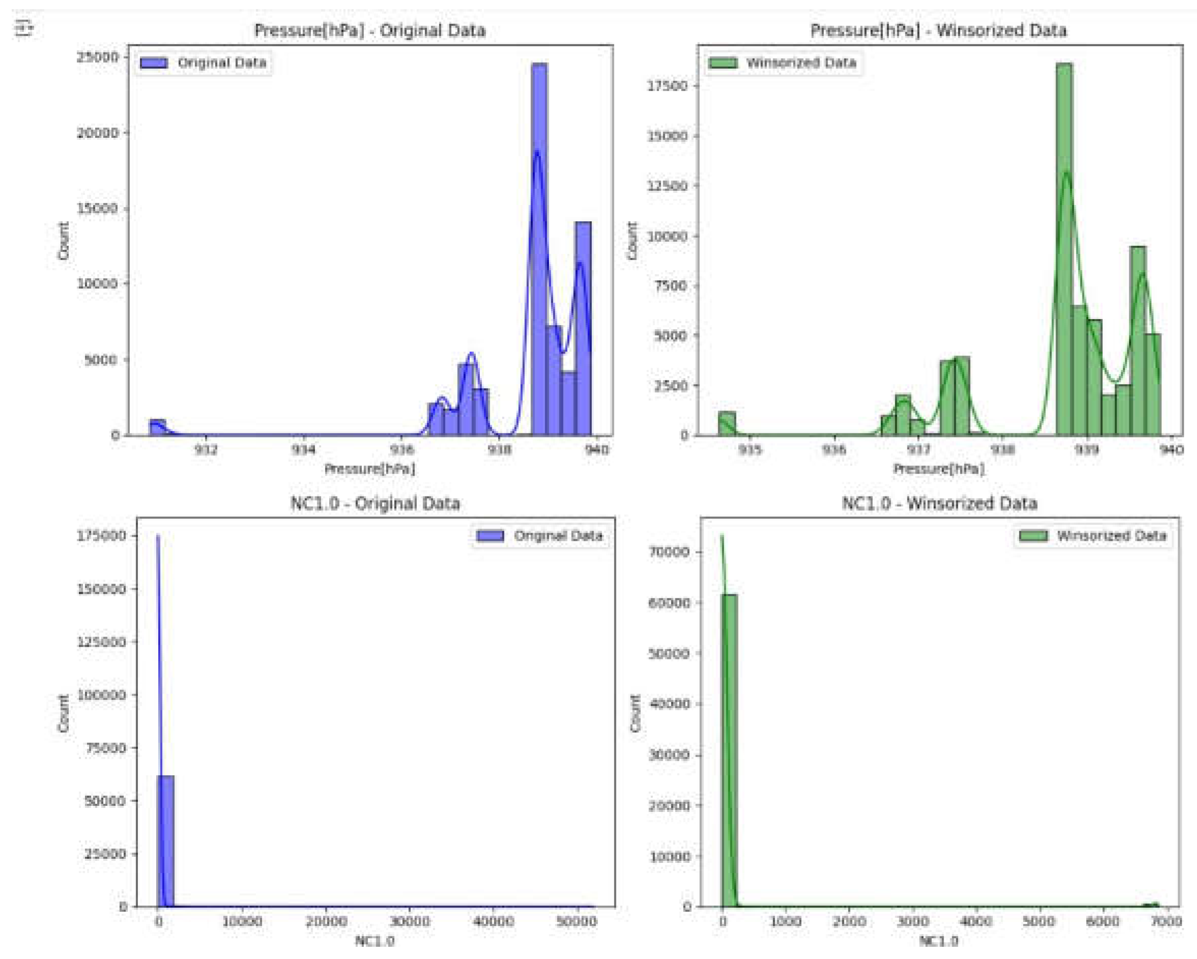
Figure 8. Correlation Matrix before winsorisation.

Figure 8. Correlation Matrix before winsorisation.

Figure 9. Correlation Matrix after winsorisation.

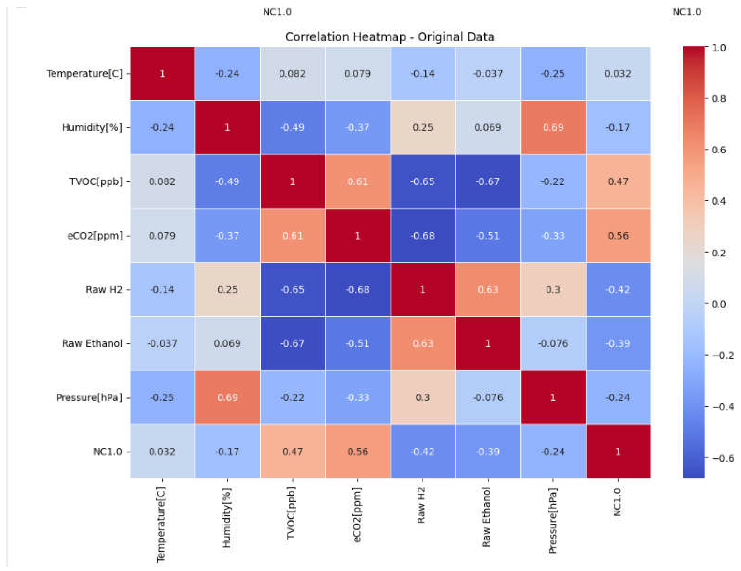
Figure 9. Correlation Matrix after winsorisation.

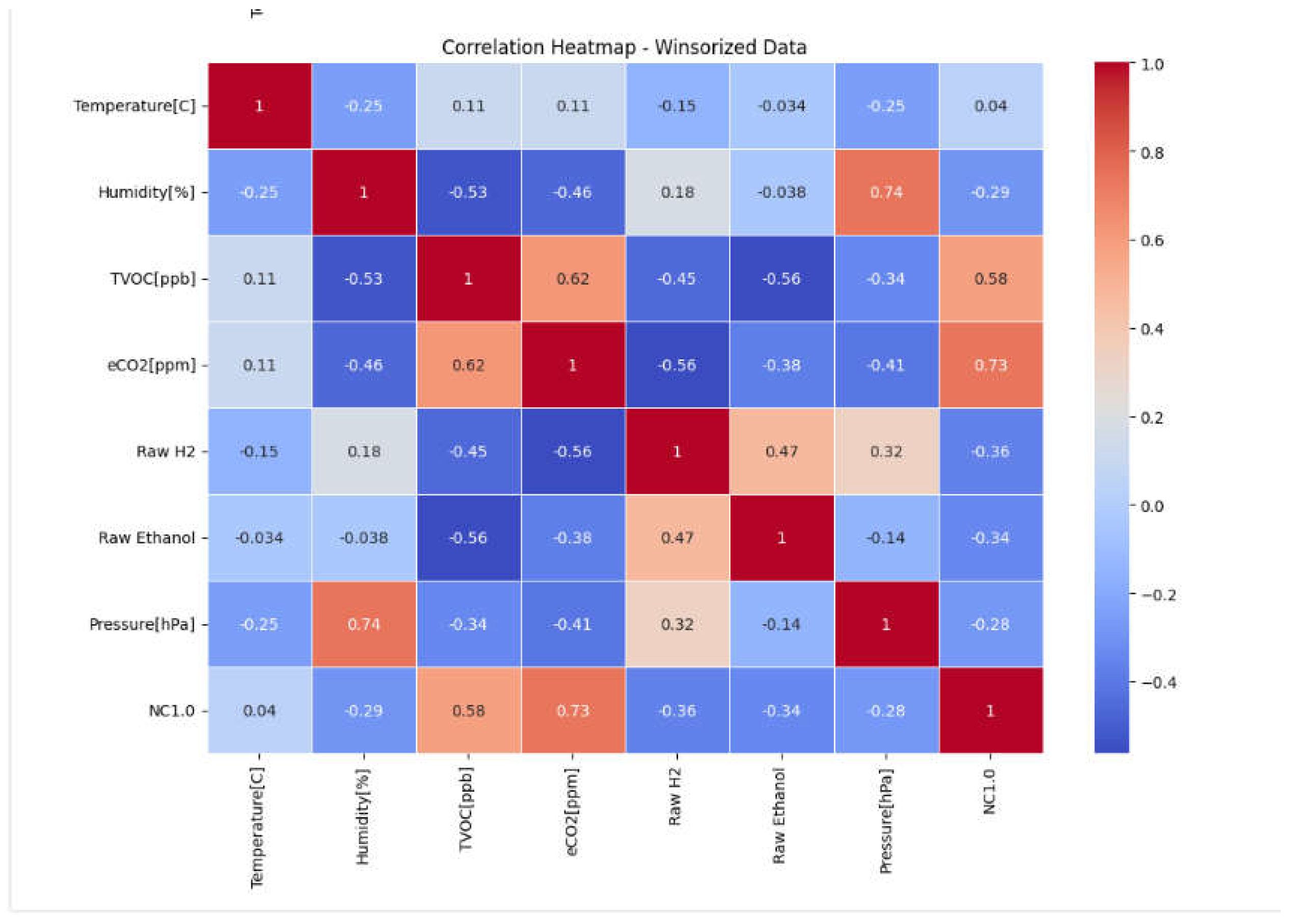
We can see that the coefficient is changed a bit but not excessively Moreover, the histograms some of the features had some change and the kde to look at overall distributions for some features they underwent significant changes in their kde like H2 and Temperature. Hence, the next step is to train a model on both datasets to verify whether the outliers have affected the model or not.

Figure 10. Output for Accuracy Scores, cross validation matrix before and after winsorisation with confusion matrix before winsorisation.

Figure 10. Output for Accuracy Scores, cross validation matrix before and after winsorisation with confusion matrix before winsorisation.

Figure 11. Confusion matrix before and after winsorisation

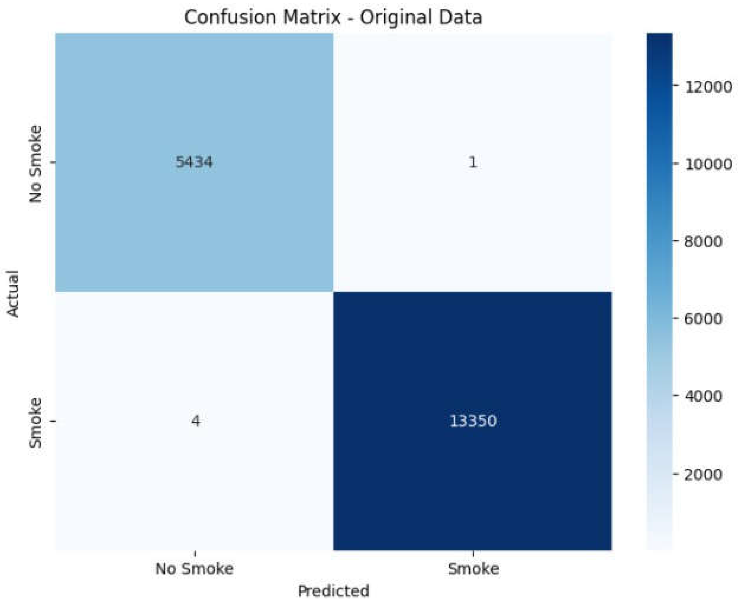
Figure 11. Confusion matrix before and after winsorisation

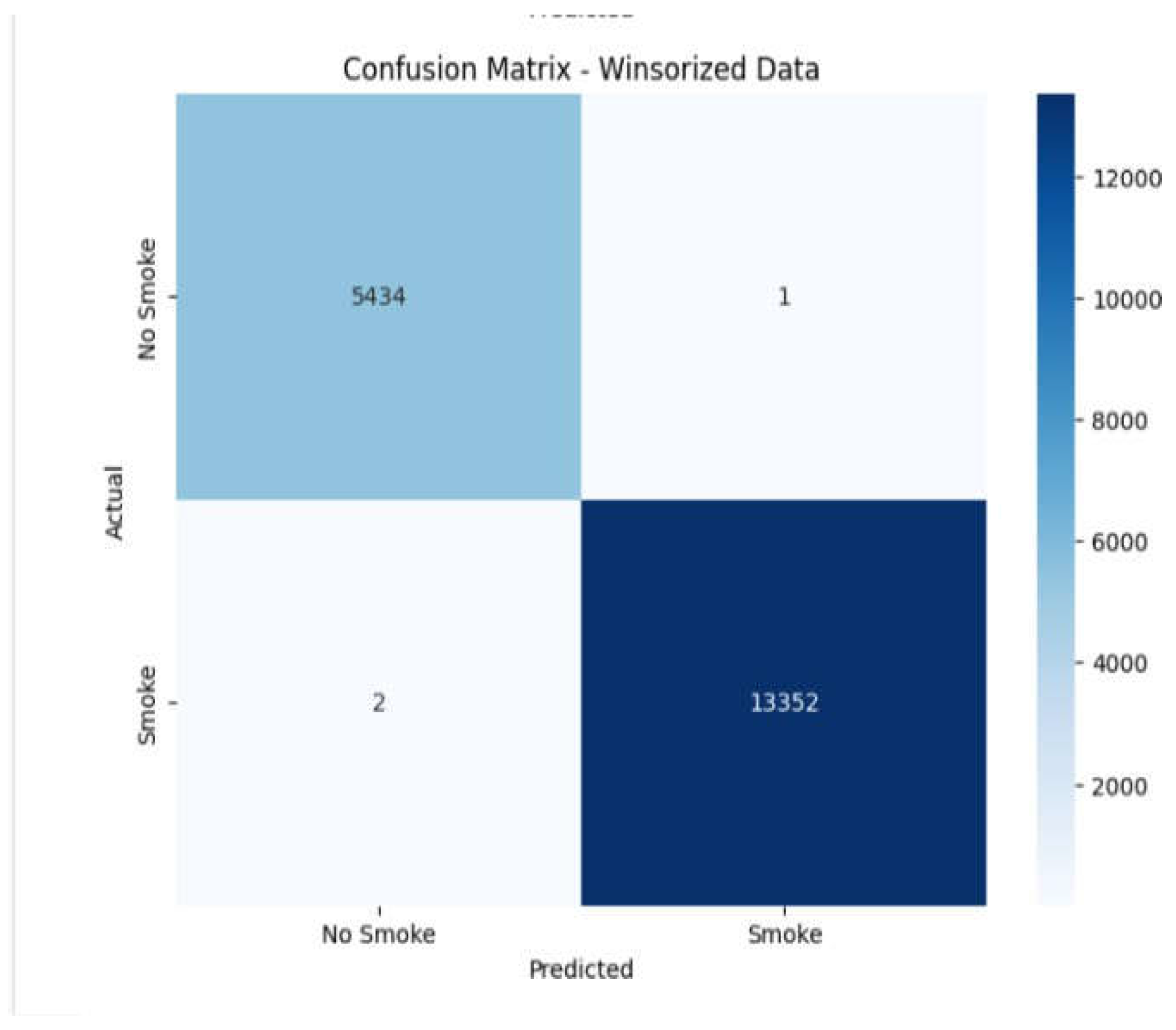
As can be seen in shown results in the score of cross validation and confusion matrix scores and scores of cross validations in order to evaluate the test model there is negligible change that means the outliers have not perturbed performance of the model and its prediction.

EDA (Exploratory Data Analysis) 

Exploratory data analysis provides context to the understanding of the datasets that it assists with in terms of uncovering pattern, relationship and any outliers that can affect the model and these can provide vital insight into feature selection and engineering.

Pair plot: 

A pair plot has been plotted to determine the top features from the pre-processed data of the pair plot we can see relationship which pair of features there is a notable trend or correlation. For the code since the dataset had more than 60000 records it was impossible to run on google Colab since it hung after consuming all the computer RAMit has been established that 10000 random records using sampling technique was a sufficient number to at least pick up the type of trends, correlation and pattern among the features.

Figure 12. Code to limit pair plot rows and plot pair plot

Figure 12. Code to limit pair plot rows and plot pair plot

Figure 13. Output of pair plot code

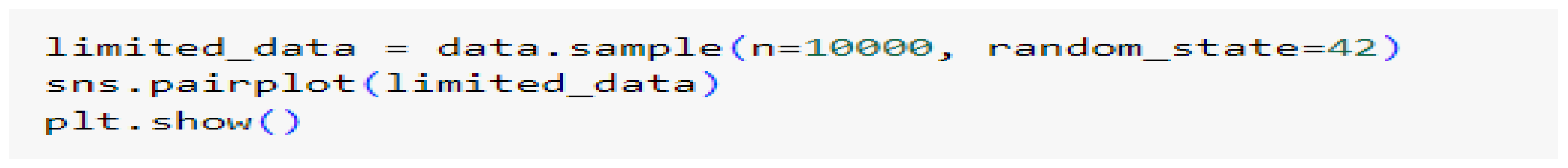
Figure 13. Output of pair plot code

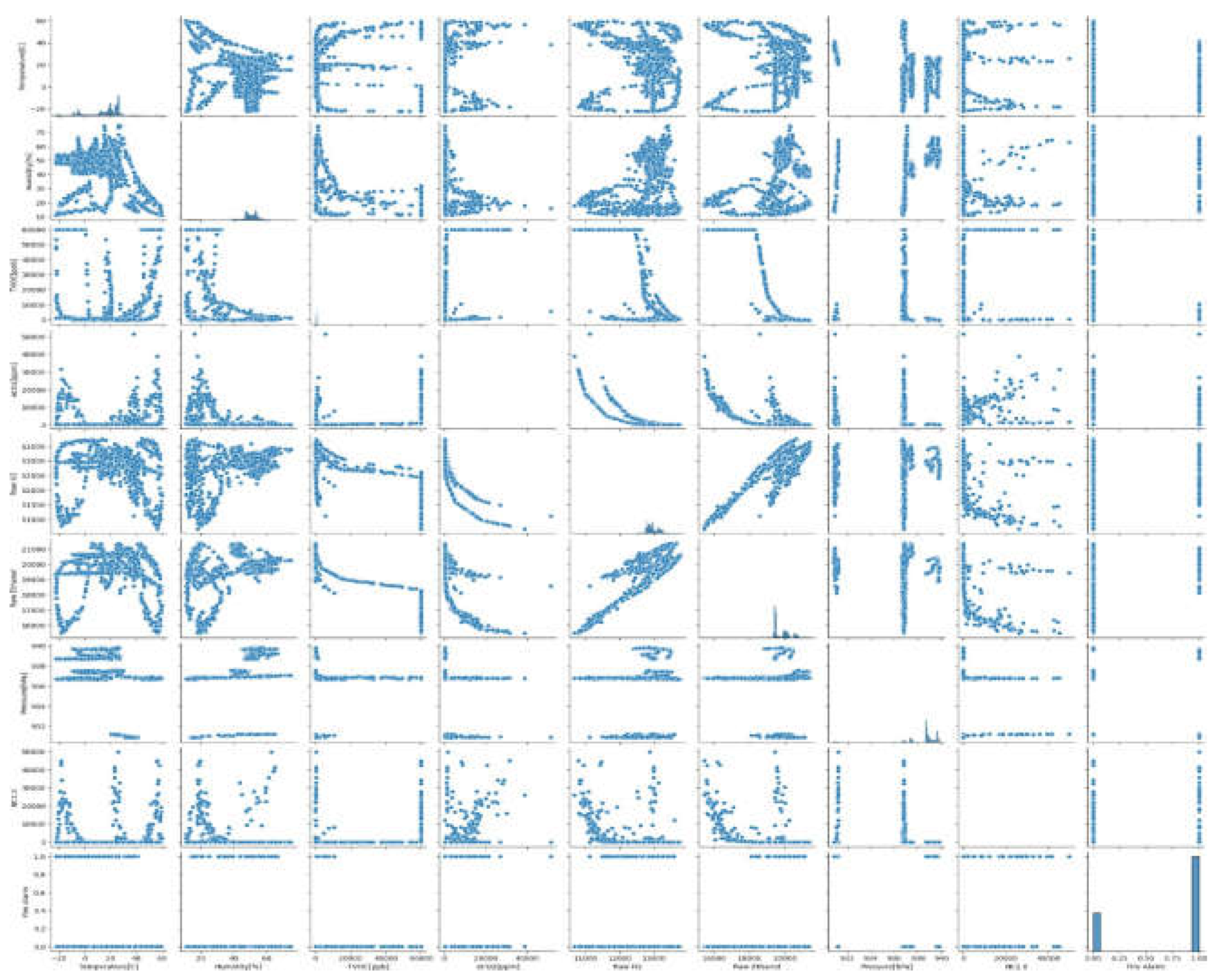
From the pair plot analysis, there have been some important feature relationships that have been identified:

• Temperature and Humidity: These two variables have a negative relationship as rising temperatures are likely to be followed by decreasing humidity, particularly in fire cases where heat evaporates water content in the air.
• TVOC and eCO₂: These two features have a weak positive correlation with each other because both are released during burning events. As a fire continues to grow, high levels of total volatile organic compounds (TVOC) and equivalent carbon dioxide (eCO₂) can be indicators of the occurrence of active burning.
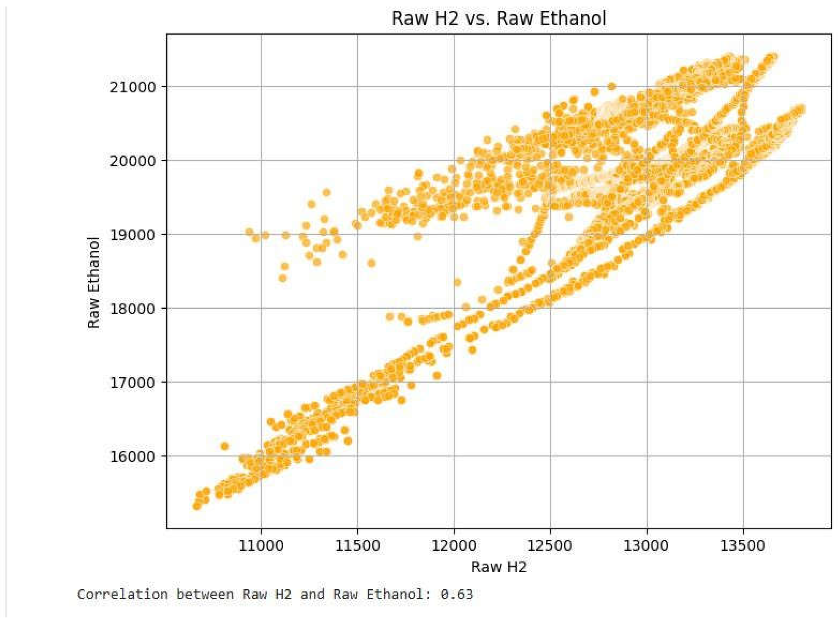
• H₂ and Ethanol: Both of these gases also share a positive correlation because they are usually released in large quantities together during a fire. They rise together and hence are effective in detecting smoke and fire accidents.

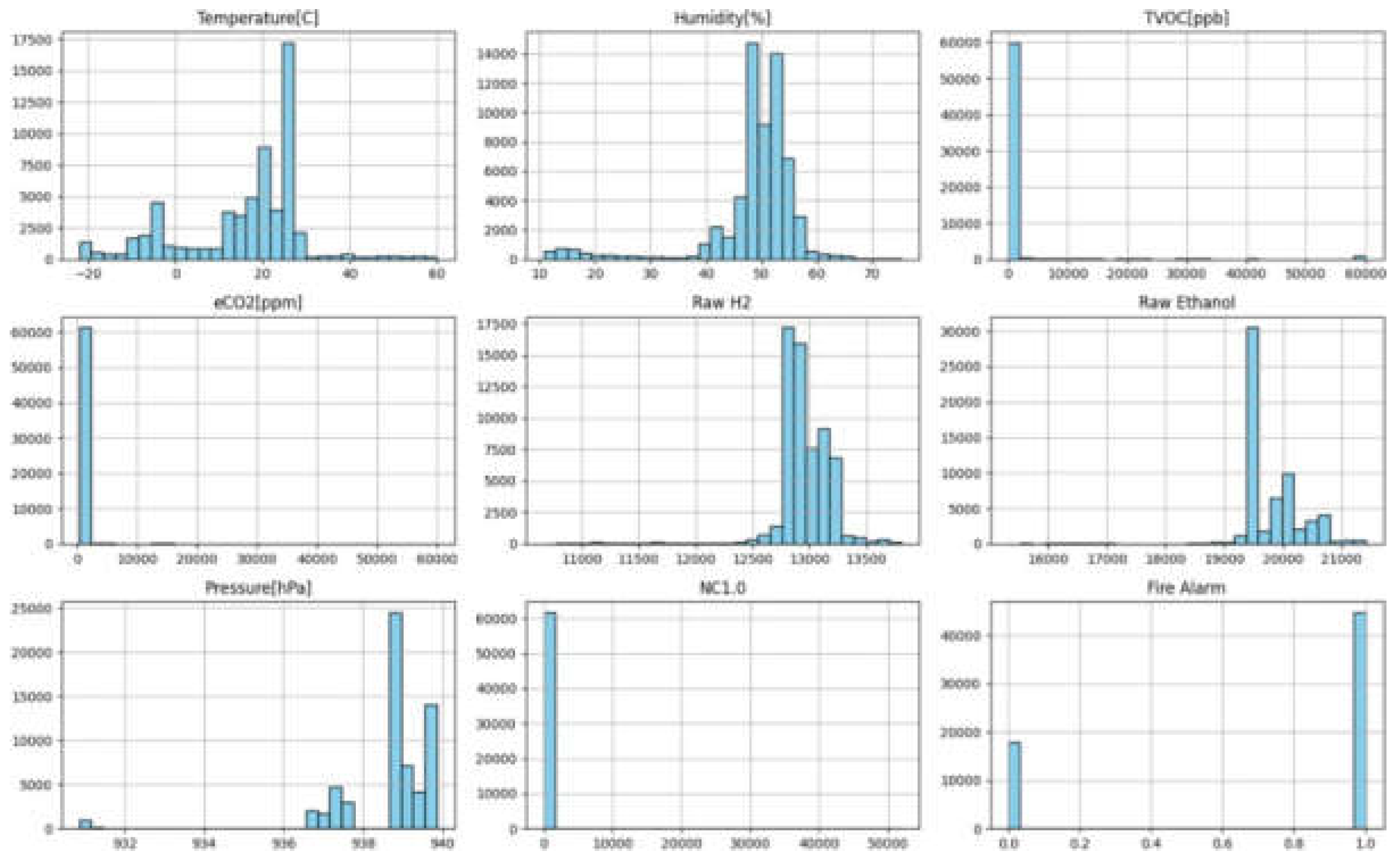
Histograms: 

To For exploring the distribution of individual characteristics and finding out if there are issues such as outliers or skewness, histograms are employed. Histograms provide feedback regarding feature scaling requirements and indicate any anomalies in the data that may need correction. Histograms also pick out features that may require imputation for missing values. Based on the dataset, histograms for each variable are plotted using Matplotlib, which allows for an easy visualization of feature distributions.

Figure 14. Output for histograms for features in dataset.

Figure 14. Output for histograms for features in dataset.

Scatterplots: 

Scatterplots are used to identify patterns and clusters between specific pair of features that were chosen to enable the recognition of linear and non-linear relationships. Scatter plots tend to provide an intuitive understanding of features relationship that can add support to feature engineering. Scatter plots can even detect outliers.

Figure 15. Output to Plot Scatter plot and correlation value for TVOC and eCO2.

Figure 15. Output to Plot Scatter plot and correlation value for TVOC and eCO2.

Figure 16. Output to Plot Scatter plot and correlation value for TVOC and eCO2.

Figure 16. Output to Plot Scatter plot and correlation value for TVOC and eCO2.

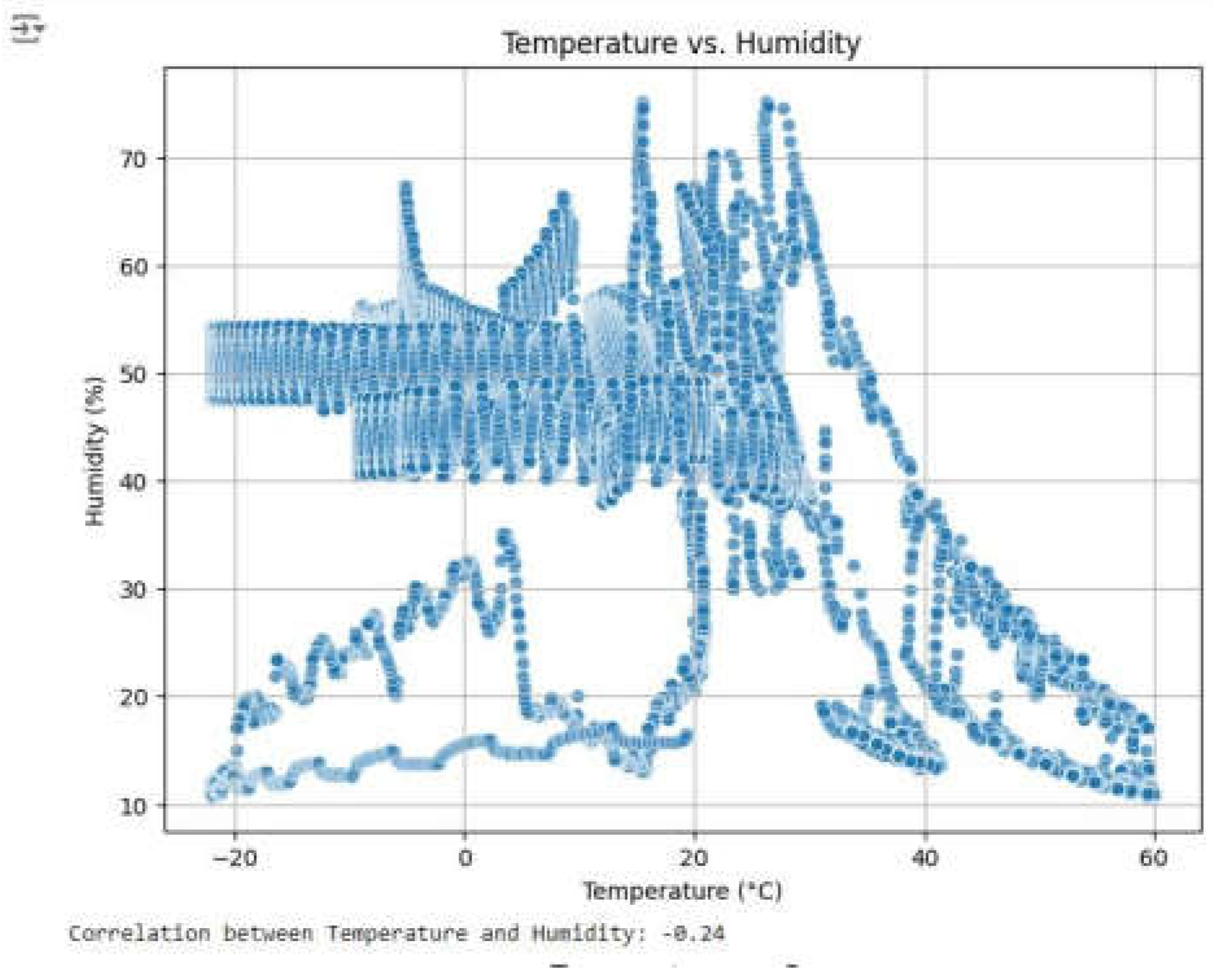
Figure 17. Output to Plot Scatter plot and correlation value for Raw H2 and Raw Ethanol.

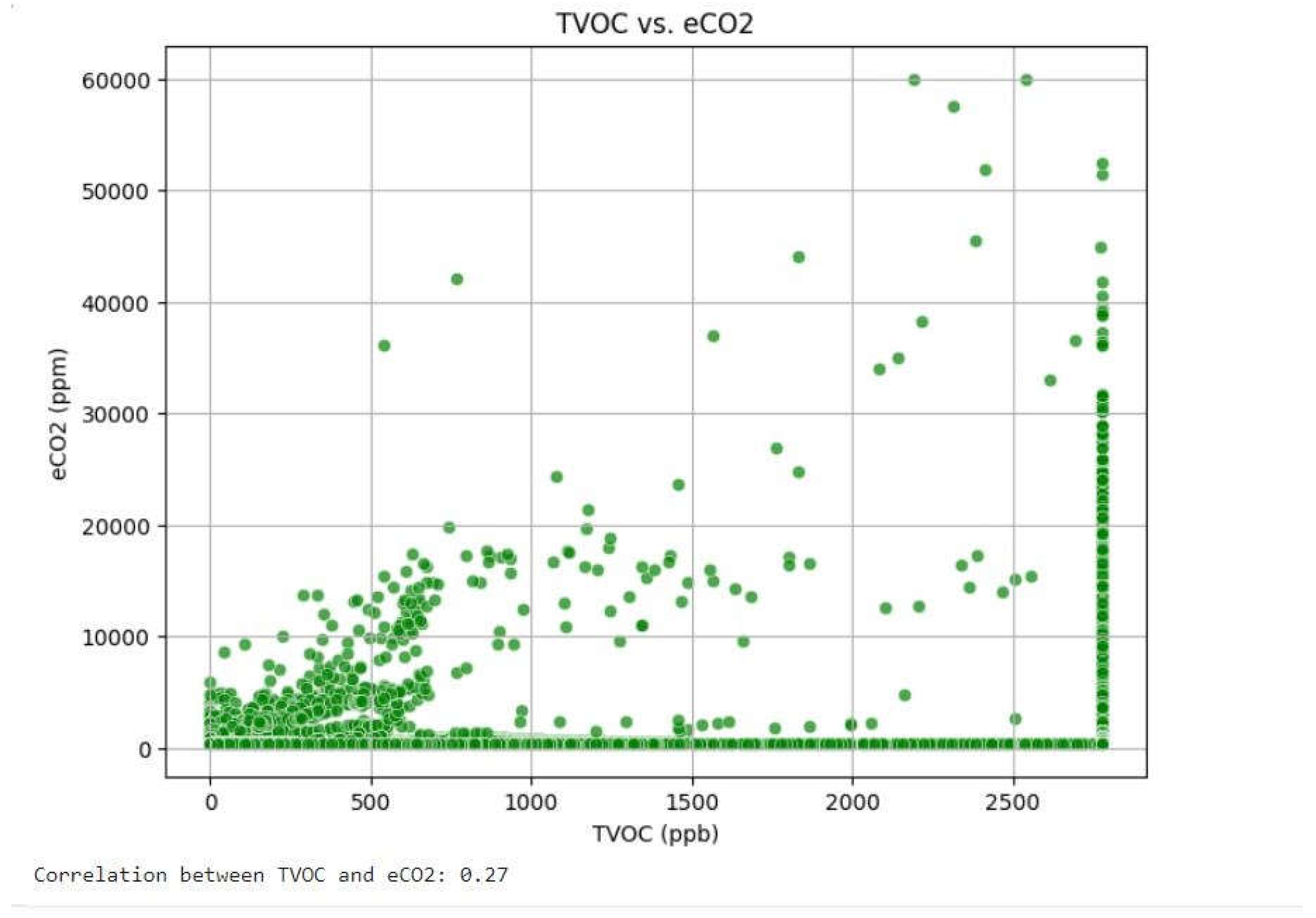
Figure 17. Output to Plot Scatter plot and correlation value for Raw H2 and Raw Ethanol.

Multiple Models 

Three machine learning algorithms were selected to determine the optimal approach for the dataset, each being picked due to its specific advantage. Since the dataset contained no missing values, algorithms such as K-Nearest Neighbors (KNN) and K-Means were not ideal since they rely on distance-based calculations that might not produce the optimal outcome.

Decision Tree Classifier: This classifier can effectively capture intricate feature and target variable relationships. It can handle non-linear relationships in the data very well and is therefore a good choice for fire detection.

Logistic Regression: Selected because of its ease and efficiency, logistic regression is effective for linearly separable data. It is most appropriate for binary classification problems, such as defining the fire alarm status as 0 (no fire alarm on) or 1 (fire alarm on).

Random Forest Classifier: Being an ensemble learning method, Random Forest integrates multiple decision trees in order to enhance accuracy, avoid overfitting, and enhance generalization. The model is most robust against noise and variability in data and is thus a good option for precise fire detection.

Cross validation 

Cross-validation is employed to test the performance of all the models while ensuring they generalize well to new, unseen data. In this study, a 5-fold cross-validation approach is employed, where the dataset is divided into five folds. Four folds are used for training, and the remaining one is used as the test set. It is done five times, with each fold taking turns being the test set. The primary objective is to check model robustness and prevent overfitting.

Figure 18. Output to cross- validate multiple models.

Figure 18. Output to cross- validate multiple models.

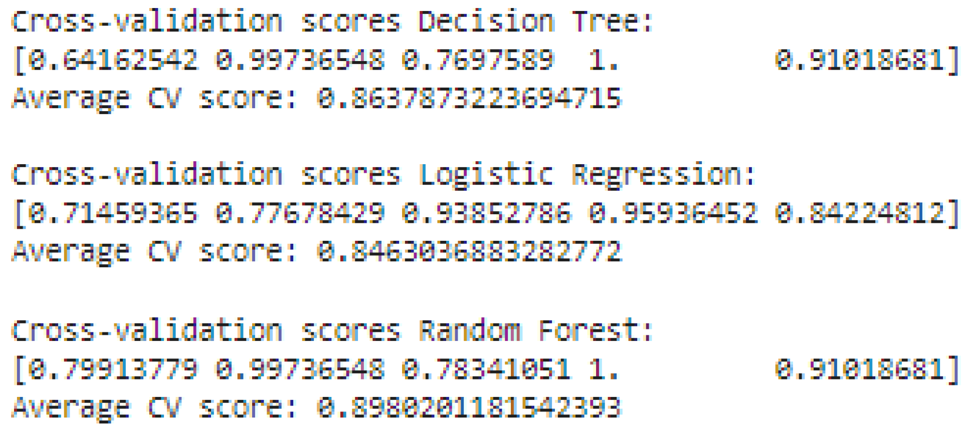
The results indicate that the Random Forest model achieved the best cross-validation score, indicating its ability to generalize well across different subsets of the data and not overfit. Logistic Regression achieved the worst score, due to the fact that it is not able to capture complex non-linear relationships. Random Forest also outperformed the Decision Tree model since it is an ensemble of numerous decisions trees and averages their predictions, thus leading to improved accuracy and stability.

Model Validation and Evaluation

Confusion Matrix

To further assess model performance, a confusion matrix is generated for each classifier. The confusion matrix provides a visual summary of correctly and incorrectly classified instances and helps in identifying patterns in model errors. Heatmaps are used to display the results for each model.

Figure 19. Output to confusion matrix for decision tree and logistic regression.

Figure 19. Output to confusion matrix for decision tree and logistic regression.

Figure 20. Output to confusion matrix for Random Forest tree.

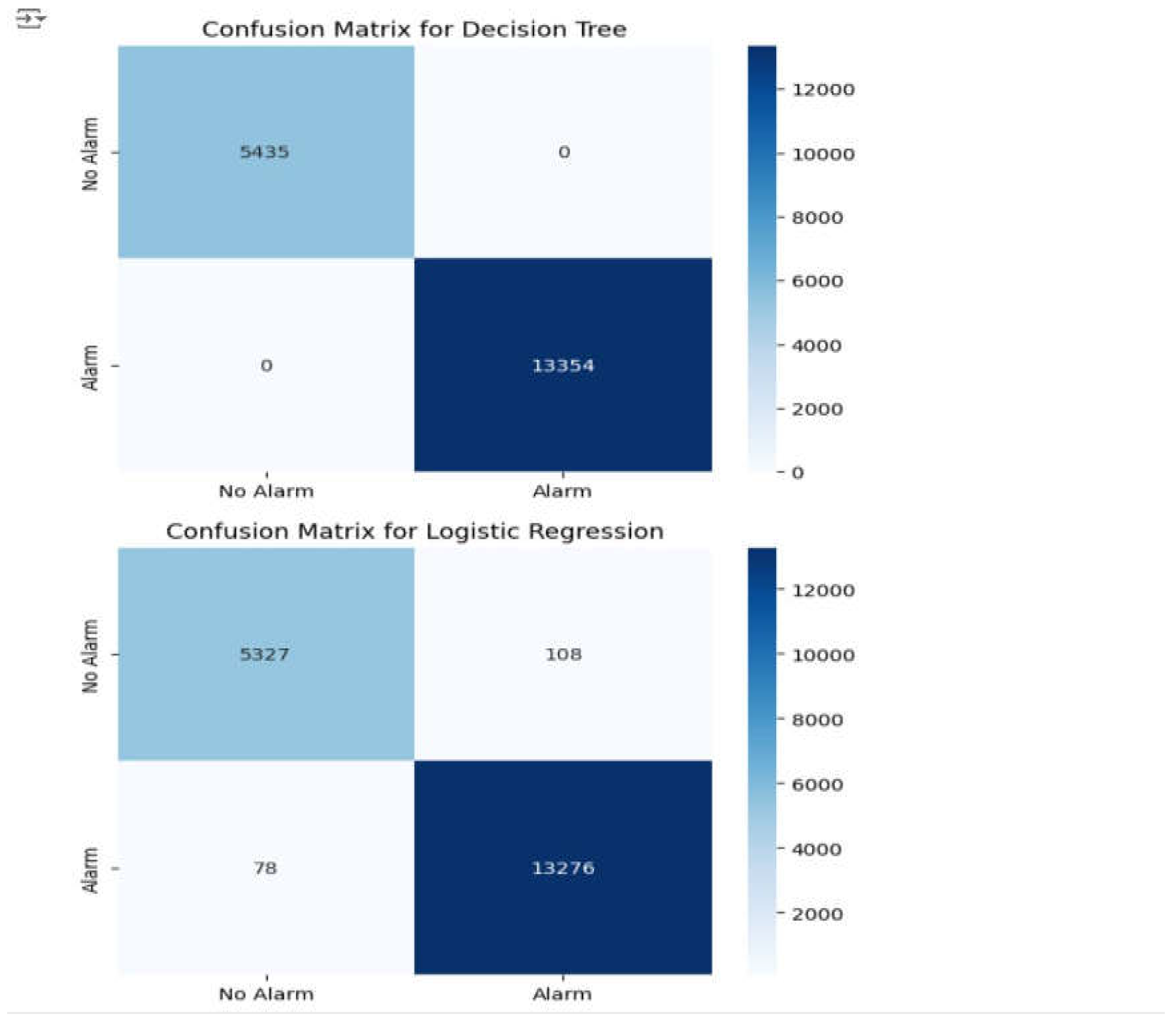
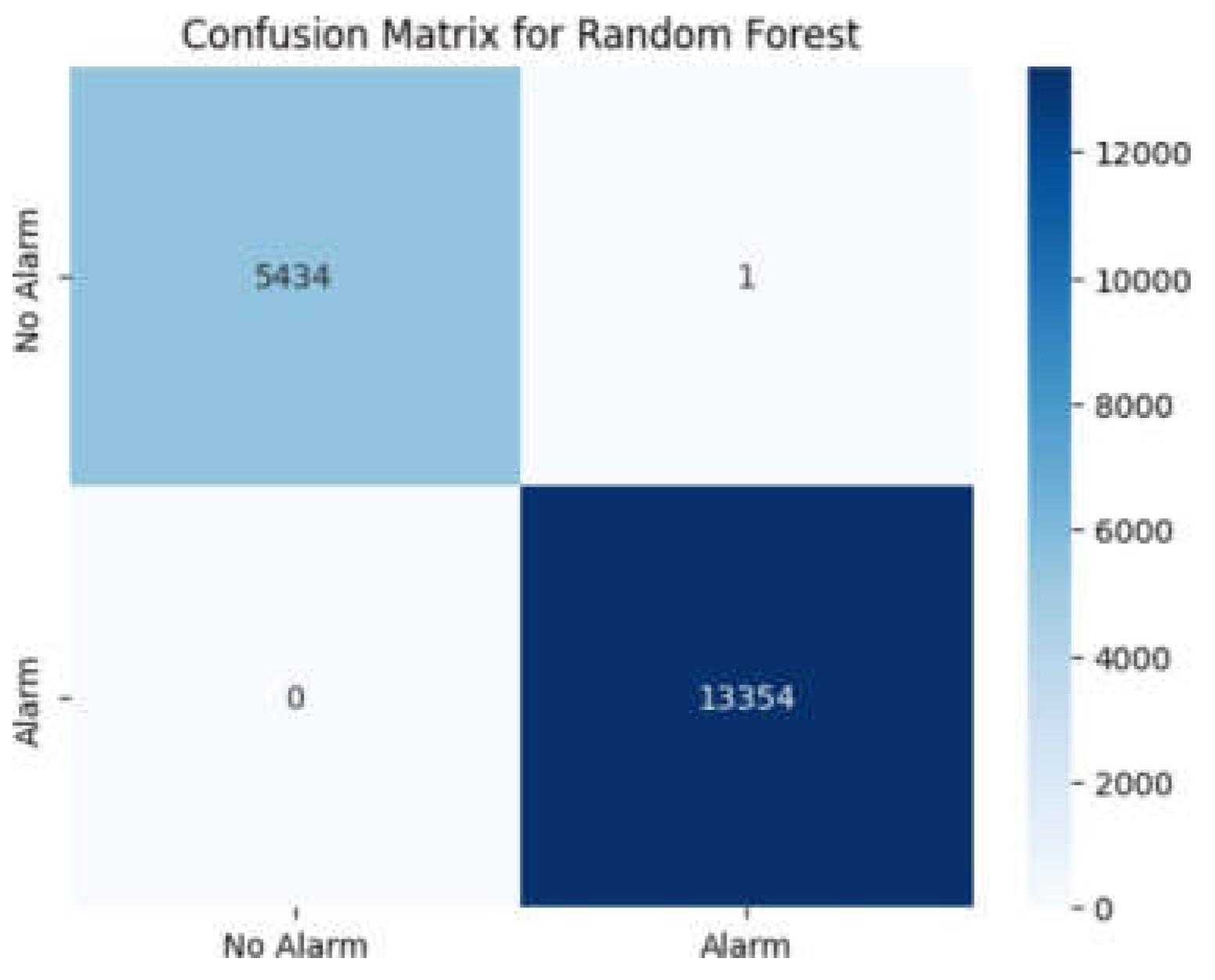
Figure 20. Output to confusion matrix for Random Forest tree.

Classification Report

A classification report is generated to provide precise performance metrics, such as:

Accuracy: The global accuracy of model predictions.

Precision: The proportion of positive predicted cases that are correct in all predicted positive cases.

Recall: The proportion of actually positive cases correctly predicted by the model.

F1-Score: The harmonic means of precision and recall, providing an even metric of model performance.

Figure 21. Classification reports for a number of models.

Figure 21. Classification reports for a number of models.

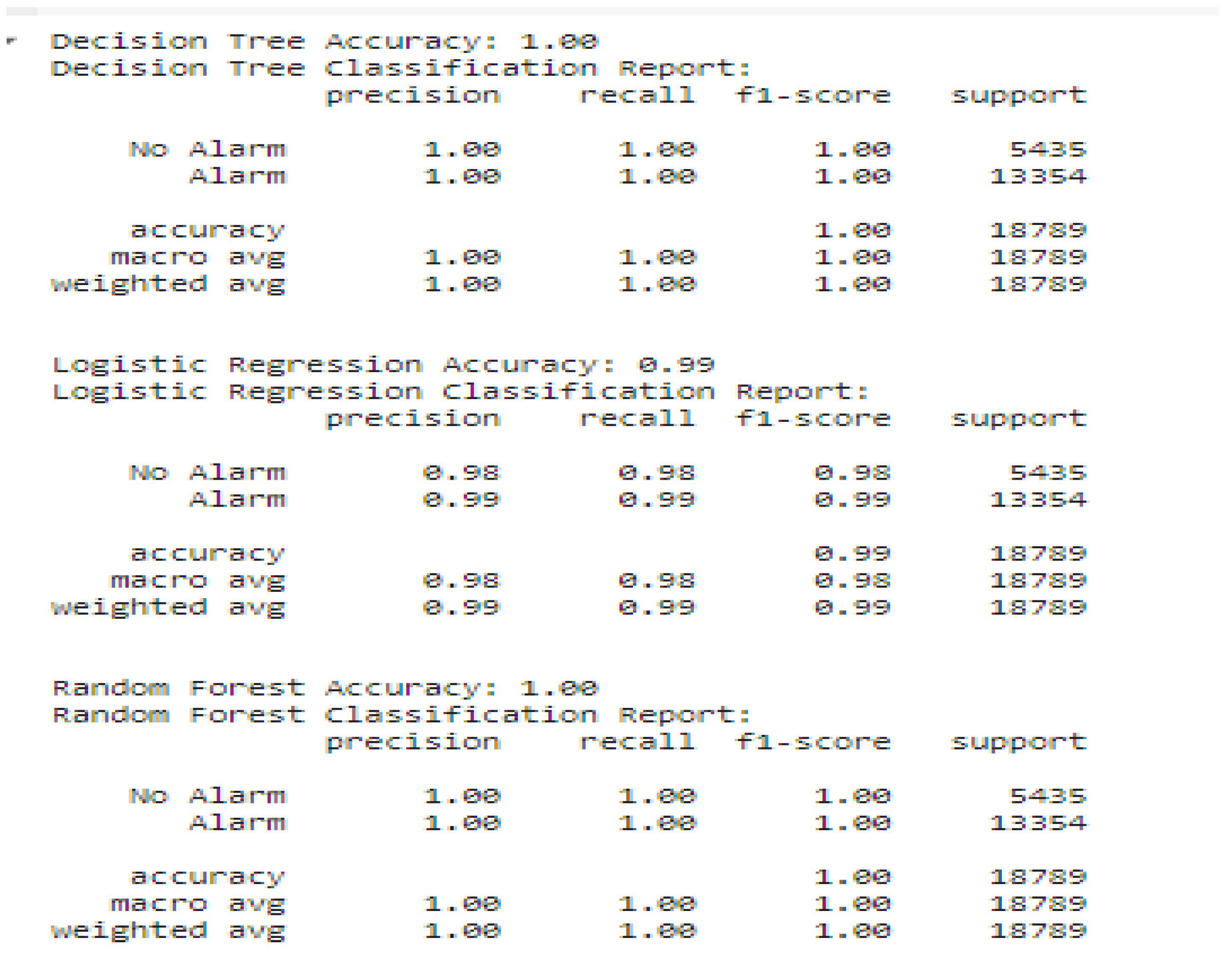
The results point to the fact that Random Forest and Decision Tree models outperformed Logistic Regression by approximately 0.02%. The models were very accurate in making correct positive predictions, and in being very high in recall, indicating their ability in true positive case identification. The F1-score confirms the strong precision vs. recall balance, and the support measure confirms the correct number of instances classified per category. Overall, the Random Forest model performs better and thus is ideal for accurate detection of fires.

8. Conclusion and Findings:

Throughout the whole code it can be seen that the Kaggle dataset was perfect and handled nicely so there were not a lot of issues and no missing data with the dataset, and it has ensured there's no overfitting by cross-validation scores. Hence, due to safety concerns and not considering financial costs in decision-making the ideal model is the random forest classifier model because with its high accuracy and it encompasses an ensemble of the decision trees classifier and hence having less overfitting tendency and it performed better than logistic regression by attaining better accuracy and cross validation scores. However, the model has fewer constraints such as costly monetary spending on the computer systems and is not compatible with other models so one can apply logistic regression since it is more balanced with a correctness rate of 90%. The other important finding one can see here is that the outliers haven't had any impact on the performance of the models so it would have been fine if they were not treated specially.

9. Conclusions

The dataset was first validated by using data.head() to examine its structure and data.describe() to generate overall statistics summaries. After the dataset had been validated, it was pre-processed using various techniques in order to enhance the performance of the model. Preprocessing included importing necessary libraries for handling the data and analysis, missing values handling for the sake of completeness of the data, and elimination of redundant or highly correlated features by correlation analysis and visualization for the purpose of preventing multicollinearity. The data was then split into test and training subsets to evaluate model performance correctly. Feature scaling through the Standard Scaler was applied to normalize feature values in order to prevent larger magnitude features from overpowering smaller features. Handling and detecting outliers were also performed using Winsorisation in order to decrease extreme values' effects, with further analysis conducted on whether outliers significantly influenced model performance.

Following preprocessing, Exploratory Data Analysis (EDA) was conducted to discover underlying patterns and relationships within the data. This included using scatter plots to visualize feature relationships and correlations, correlation matrices to identify feature dependencies and select the most influential variables, and histograms to examine feature distributions in the observation of skewness and outliers. Following EDA, various machine learning models were trained and tested, including Random Forest, Decision Tree, and Logistic Regression. Every model was cross validated to ensure generalization and detect any potential overfitting, confusion matrices to validate the classification accuracy, and classification reports to analyze the key performance metrics such as precision, recall, and support to determine the best model for fire detection. The final test revealed that Random Forest was best in terms of accuracy and generalization compared to the other models and was most appropriate for use in fire detection. Decision Tree and Logistic Regression were also appropriate and useful based on the needs of a given scenario.

References

- White, L.; Ajax, R. Improved Fire Detection and Alarm Systems. 2025. [Google Scholar]
- Khan, A. A., Zhang, T., Huang, X., & Usmani, A. (2023). Machine learning driven smart fire safety design of false ceiling and emergency response. Process Safety and Environmental Protection, 177, 1294-1306. [CrossRef]
- Yar, H., Khan, Z. A., Rida, I., Ullah, W., Kim, M. J., & Baik, S. W. (2024). An efficient deep learning architecture for effective fire detection in smart surveillance. Image and Vision Computing, 145, 104989. [CrossRef]
- Jana, S., & Shome, S. K. (2023). Hybrid ensemble based machine learning for smart building fire detection using multi modal sensor data. Fire technology, 59(2), 473-496. [CrossRef]
- Zhang, L., Mo, L., Fan, C., Zhou, H., & Zhao, Y. (2023). Data-driven prediction methods for real-time indoor fire scenario inferences. Fire, 6(10), 401. [CrossRef]
- Sousa Tomé, E., Ribeiro, R. P., Dutra, I., & Rodrigues, A. (2023). An online anomaly detection approach for fault detection on fire alarm systems. Sensors, 23(10), 4902. [CrossRef]
- Desikan, J., Singh, S. K., Jayanthiladevi, A., Singh, S., & Yoon, B. (2025). Dempster Shafer-empowered Machine Learning-based Scheme for Reducing Fire Risks in IoT-enabled Industrial Environments. IEEE Access, (99), 1-1. [CrossRef]
- Shrivastava, A.; Gogoi, A.; Shahi, S.; Chaitanya, S. IoT Enabled Real Time Fire Monitoring and Response in Urban Areas. Information Sciences and Technological Innovations 2024, 1, 19–27. [Google Scholar]
- Kim, Y. J., & Kim, W. T. (2022). Uncertainty assessment-based active learning for reliable fire detection systems. IEEE Access, 10, 74722-74732. [CrossRef]
- Martinsson, J., Runefors, M., Frantzich, H., Glebe, D., McNamee, M., & Mogren, O. (2022). A novel method for smart fire detection using acoustic measurements and machine learning: proof of concept. Fire technology, 58(6), 3385-3403. [CrossRef]
- Bian, H., Zhu, Z., Zang, X., Luo, X., & Jiang, M. (2022). A CNN based anomaly detection network for utility tunnel fire protection. Fire, 5(6), 212. [CrossRef]
- Kim, H. C., Lam, H. K., Lee, S. H., & Ok, S. Y. (2024). Early Fire Detection System by Using Automatic Synthetic Dataset Generation Model Based on Digital Twins. Applied Sciences, 14(5), 1801. [CrossRef]
- Jena, K. K., Bhoi, S. K., Malik, T. K., Sahoo, K. S., Jhanjhi, N. Z., Bhatia, S., & Amsaad, F. (2022). E-learning course recommender system using collaborative filtering models. Electronics, 12(1), 157. [CrossRef]
- Aherwadi, N., Mittal, U., Singla, J., Jhanjhi, N. Z., Yassine, A., & Hossain, M. S. (2022). Prediction of fruit maturity, quality, and its life using deep learning algorithms. Electronics, 11(24), 4100. [CrossRef]
- Kumar, M. S., Vimal, S., Jhanjhi, N. Z., Dhanabalan, S. S., & Alhumyani, H. A. (2021). Blockchain-based peer-to-peer communication in autonomous drone operation. Energy Reports, 7, 7925-7939. [CrossRef]
- Saeed, S., & Haron, H. (2021). A systematic mapping study of low-grade tumor of brain cancer and CSF fluid detecting approaches and parameters. Approaches and Applications of Deep Learning in Virtual Medical Care, 1(1), 1-30. [CrossRef]
- Saeed, S., Abdullah, A., Jhanjhi, N. Z., Naqvi, M., & Ahmed, S. (2020). Effects of cell phone usage on human health and specifically on the brain. In Machine learning for healthcare (pp. 53-68). Chapman and Hall/CRC. [CrossRef]
- Saeed, S., Jhanjhi, N. Z., Naqvi, M., Humayun, M., & Ponnusamy, V. (2021). Quantitative analysis of COVID-19 patients: A preliminary statistical result of deep learning artificial intelligence framework. In ICT solutions for improving smart communities in Asia (pp. 218-242). [CrossRef]
- Saeed, S., Jhanjhi, N. Z., Naqvi, S. M. R., & Khan, A. (2022). Cost optimization of software quality assurance. In Deep learning in data analytics: Recent techniques, practices, and applications (pp. 241–255). [CrossRef]
- Saeed, S., Jhanjhi, N. Z., Naqvi, S. M. R., & Khan, A. (2022). Analytical approach for security of sensitive business cloud. In Deep learning in data analytics: Recent techniques, practices, and applications (pp. 257–266). [CrossRef]
- Saeed, S., Jhanjhi, N. Z., Naqvi, M., Ponnusamy, V., & Humayun, M. (2020). Analysis of climate prediction and climate change in Pakistan using data mining techniques. In Industrial Internet of Things and cyber-physical systems: Transforming the conventional to digital (pp. 321–338). [CrossRef]
- Aldughayfiq, B., Ashfaq, F., Jhanjhi, N. Z., & Humayun, M. (2023). Explainable AI for retinoblastoma diagnosis: interpreting deep learning models with LIME and SHAP. Diagnostics, 13(11), 1932. [CrossRef]
- Attaullah, M., Ali, M., Almufareh, M. F., Ahmad, M., Hussain, L., Jhanjhi, N., & Humayun, M. (2022). Initial stage COVID-19 detection system based on patients’ symptoms and chest X-ray images. Applied Artificial Intelligence, 36(1), 2055398. [CrossRef]
- Lee, S., Abdullah, A., & Jhanjhi, N. Z. (2020). A review on honeypot-based botnet detection models for smart factory. International Journal of Advanced Computer Science and Applications, 11(6). [CrossRef]
- Shah, I. A., Jhanjhi, N. Z., & Laraib, A. (2023). Cybersecurity and blockchain usage in contemporary business. In Handbook of Research on Cybersecurity Issues and Challenges for Business and FinTech Applications (pp. 49-64). IGI Global. [CrossRef]
- Muzafar, S., & Jhanjhi, N. Z. (2020). Success stories of ICT implementation in Saudi Arabia. In Employing Recent Technologies for Improved Digital Governance (pp. 151-163). IGI Global. [CrossRef]
- Gill, S. H., Razzaq, M. A., Ahmad, M., Almansour, F. M., Haq, I. U., Jhanjhi, N. Z., … & Masud, M. (2022). Security and privacy aspects of cloud computing: a smart campus case study. Intelligent Automation & Soft Computing, 31(1), 117-128. [CrossRef]
Disclaimer/Publisher’s Note: The statements, opinions and data contained in all publications are solely those of the individual author(s) and contributor(s) and not of MDPI and/or the editor(s). MDPI and/or the editor(s) disclaim responsibility for any injury to people or property resulting from any ideas, methods, instructions or products referred to in the content. |
© 2025 by the authors. Licensee MDPI, Basel, Switzerland. This article is an open access article distributed under the terms and conditions of the Creative Commons Attribution (CC BY) license (http://creativecommons.org/licenses/by/4.0/).
Copyright: This open access article is published under a Creative Commons CC BY 4.0 license, which permit the free download, distribution, and reuse, provided that the author and preprint are cited in any reuse.