
Submitted:
09 April 2025
Posted:
10 April 2025
You are already at the latest version
Abstract
This study aims to verify whether there is any relationship between the different classification outputs produced by distinct ML algorithms and the relevance of the data they classify, for addressing the problem of the knowledge extraction (KE) from datasets. If such relationship existed, the main objective of this research is to use it in order to improve performance in the important task of KE from datasets. A new dataset generation and a new ML classification measurement methodology were developed to check whether the feature subsets (FSs) best classified by a specific ML algorithm correspond to the most KE-relevant combinations of features. Medical expertise was extracted to check knowledge relevance using two LLMs, namely chat GPT and Google Gemini. Some specific ML algorithms fit much better than others for a working dataset extracted from a given probability distribution. They best classify FSs that contain combinations of features particularly knowledge relevant. This implies that using a specific ML algorithm we can indeed extract useful scientific knowledge. The best-fitting ML algorithm is not known a priori. However, we can bootstrap its identity using a small amount of medical expertise, and we have a powerful tool for extracting (medical) knowledge from datasets using ML.
Keywords:
knowledge relevance
; knowledge extraction
; feature subset
; large language models
; machine learning algorithms
; statistics
1. Introduction
Each ML algorithm produces a different output for the same input. The input may be a whole dataset or a subset of the features (FS) of the dataset. The classifying power may be interpreted as the ‘goodness’ of the FS.
However, there exists some confusion about the meaning of ‘goodness’ in this context. Usually it means FSs that are useful to build a good predictor (of the class of the dataset, i.e. performing a high classification score). On the other hand, it means finding all potentially relevant features [1]. This relevance vs. usefulness distinction is not always well discriminated and depends a lot on what we mean by relevance [2,3].
No better-than-the-others ML algorithm is available. However, their different classification results may have some meaning. If we encode (medical) knowledge for a given dataset, we may check if different classifying algorithms behave better than others do, with respect to knowledge relevance, in order to extract such encoded knowledge.
The aim of this paper is to encode medical knowledge relevance to test if there are significant differences among ML algorithms to learn that knowledge and if so to use the most efficient ML algorithm on a given dataset for massively extracting useful and relevant medical knowledge out of it.
A secondary objective of this research is to assess the quality of datasets using ML i.e. to test if the different ML algorithms cannot learn knowledge out of them because they are not well formed for whatever reason.
2. Materials and Methods
In this section, we first introduce a methodology to validate an original dataset using a probability distribution of datasets extracted from it, and then apply the methodology to the validated original datasets.
We first introduce in section 2.1 a method to generate a probability distribution of working datasets out of an original dataset under study (see Appendix 1 for a description of the original datasets used in this research). In section 2.2, we introduce a method to compute classification performance using ordered lists of all possible combinations of FSs and six different supervised ML algorithms belonging to important scientific families of algorithms (see Appendix 2 for a description of these algorithms). In section 2.3, we introduce a method to encode scientific medical knowledge of a dataset using pairs (2-uples) of medical features knowledge relevant with respect to the class of the dataset, using two important LLMs. In section 2.4, we check the encoded medical knowledge against the ordered lists of classification performance in order to evaluate how well classify relevant knowledge the different ML algorithms. In section 2.5, we validate the probability distribution generation and the ML knowledge performance results. In section 2.6, we apply the whole methodology to the original datasets that have passed its distribution validation.
2.1. Dataset Generation over a Probability Distribution: Dataset Feature Splitting (DFS)
Because we are intending to measure knowledge relevance of FSs and then to assess its relationship to classification score of the same FSs, we need different datasets with the same features (columns) extracted from the same probability distribution i.e. holding a stationary assumption [4].
For this purpose, we have developed dataset feature splitting (DFS). It operates as follows: Let us assume that we are studying lactose intolerance in Eastern populations [5]. We would be interested in one dataset of people from the relevant East (e.g., Japan) and another from the remainder of the people not considered Eastern. For instance, if we had a dataset of people from the world and one of the features (columns) was the geographic origin (say Japan/not Japan), we would divide the dataset according to that column to obtain two different datasets, one from Japan and the other from the remainder of the world, which were extracted from the same probability distribution.
Figure 1 illustrates the process using a fragment of realistic data from one of the datasets [6] used in this study. The first column (AGE) has sorted this dataset and we have generated two different datasets (different colors) by dividing column AGE using the threshold 60 years old (younger people under 60 years and elder people over this age). Table 1 shows the methodology in systematic fashion.
In general, if we have a medical dataset of 12 medical features (except the class), we may construct a maximum of 24 different datasets dividing 2-fold across each feature (column), extracted from the same population probability distribution.
2.2. An Objective Measure of Classification performance: Ordered Lists of All Combinations of FS of a Given Size
In order to measure FS classification performance on each ML algorithm, we propose the following method.
Each ML algorithm produces a different classification results for the same FS. We need an exact measure of how well a given-sized FS classifies for a given ML algorithm. Thus, we need to compute all combinations of FS of a given size. In addition, in order to compare their classification power we build F-measure-ordered lists for each important size (3, 4, 5 and 6) and each ML algorithm.
For instance in Figure 2 we have depicted the ordered lists of four of the six algorithms [7,8] used in this study for the case of FSs of size 3. We can see that FS (3, 4, 6) has obtained different positions in the different algorithms. Thus, to test how well classifies a FS of a given size with a given ML algorithm we check its position in the corresponding ordered list (same FS size and same ML algorithm). Table 2 shows the ordered lists building methodology systematically.
2.3. Encoding Knowledge Relevance: Using Medical Expertise from LLMs
In order to check how well classify the different ML knowledge relevant FSs, we need an assessment of FS relevance extracted from some source of medical expertise.
In this study, we have queried two different LLMs [9,10] (Chat GPT [11] and Google Gemini [12]) in order to encode the knowledge relevance of pairs of features (FSs of size 2). That is, if there is a relationship between pairs of features (columns of a dataset) with respect to the medical outcome of the dataset.
For instance in the Heart Failure (HF) dataset where we have one feature diabetes (column DIA) and another feature anemia (column ANA) the posed query might look like:
“Is there a synergic relationship between diabetes and anemia to suffer heart failure?”
If such relationship exists we would tag ‘1, relevant’ the pair (2, 4) corresponding to features anemia and diabetes (see Appendix 1). Otherwise, it would be tagged ‘0, non-relevant’.
Some columns, such as DIA or ANA, are 1/0 columns in which patients have or have not this feature. Other columns are numeric (e.g., diastolic blood pressure, DBP), and their values are real numbers. In this case, the column is classified according to high or low feature values. Meaningful clinical limits were used to compute classification thresholds.
Table 3 shows the medical knowledge encoding methodology systematically.
Table 4 shows a detail of Table 16 (Results section). The CRE H dataset of the HP-UCI probability distribution represents the patients of the original HP-UCI dataset that have high levels of creatinine, after the original dataset was divided according to the CRE column into those patients with high level of creatinine (CRE H) and those with low levels (CRE L). Table 4 shows the list of features (columns) that are knowledge relevant with respect to the DFS-driving feature (CRE and ALP).
2.4. How Well Classify the Different ML Algorithms the Most Relevant Binary FSs
Now we are in a position where we can compute how well the different ML algorithms classify the medical knowledge relevant FS pairs, checking their ordinal position in the ordered lists.
From Table 4 we have, for each dataset of the probability distribution, the list of features that are knowledge relevant to the driving DFS feature of the dataset. For instance, in the HP (hepatitis C) probability distribution, dataset CRE H (high level of creatinine) has feature 4 alkaline phosphatase (ALP) as relevant.
In order to test how well features 10 (CRE) and 4 (ALP), which are mutually relevant for the Hepatitis C probability distribution, get classified; we count how high the number ‘4’ rates in the four ordered lists of the dataset CRE H (CRE is feature 10). Conversely, how high the number ’10’ rates in the four ordered lists of the dataset ALP H (ALP is feature 4).
Rather than doing this individually we count, for each dataset, how high rate the numbers of its entire relevant features compound. These numbers are summed up and averaged for each of the four ordered lists (FS sizes 3, 4, 5 and 6) and the maximum produces a best-classifying winning ML algorithm per ordered list.
Table 6 shows the specific case of the CRE H dataset. For each ordered list (FS sizes 3 through 6), there is a winning ML algorithm (leftmost) and a descending ordering of algorithms to the right.
If we assign a number of ordering for each ML algorithm (1 through 6) on each FS size, we can sum across FS sizes and obtain an ordering of algorithms for each working dataset, as summarized in Table 7, which is a detail of Table 17 in the Results section.
If we do the same thing across the whole probability distributions, we can obtain a scoring for each ML algorithm and each probability distribution as shown in Table 8 for the HP-UCI distribution.
2.5. Validation Methodology
2.5.1. Validation of Method 1 (DFS)
Each original dataset has a distribution P(X) and the working datasets extracted from them using DFS have conditional distributions P(X | Xj ≤ t) or P(X | Xj ≥ t) where t is the threshold used to divide the original dataset if feature Xj has a meaning under that threshold or over it, respectively.
In order to check if the working datasets represent the same distribution we have used the Kolmogorov-Smirnov (KS) test [13]. This is the standard statistical method to test if groups of datasets belong to the same probability distribution. The input to the KS test is one working dataset (ALP H for instance) and the original HP-UCI dataset. Then it produces a p-value per working dataset.
Table 9 (a detail of Table 19 in the Results section) shows the p-values returned by the KS test applied to the ALP H and CRE H working datasets of the HP-UCI distribution. The Benjamini-Hochberg correction [14] has been applied in order to control the expected number of false positives. It is commonly applied when the KS test is applied to a number of datasets. It sorts the p-values and applies a dynamic threshold.
2.5.2. Validation of Methods 2, 3 and 4
Table 10 shows six vectors of results, one per ML algorithm, corresponding to the averaged ordinal positions of significant features in the ordered list of each working dataset of the HP-UCI distribution and one specific FS size case, namely size 3. Using these six vectors, the statistical significance of the ordinal positions in the ordered lists has been evaluated using the Chi-squared statistical test [15]. This specific case yields a p-value of 0.0036986186.
2.6. Application of the Methodology: Knowledge Extraction from the Original Datasets
The KS and the chi-squared tests serve as a filter to rule out non-well-formed distributions. In our case only two distributions pass the test, namely HP-UCI and HF-UCI, see the Results section.
Now we know that we can apply the methodology to extract knowledge from the two original datasets that generated the two successful probability distributions.
Method 1 (DFS) was applied to generate the testing distributions so we can obviate it. We have first applied Method 2 to the two successful original datasets (HP-UCI and HF-UCI) in order to build their four ordered lists (one per FS size from 3 through 6). We can use the pairs of features produced previously by Method 3 applied to the whole probability distributions of the original datasets in order to apply Method 4 on each of the two original datasets. Now we can check for the ordinal positions of the two features of each pair in the four ordered lists. Note that now we check for pairs of features rather than for individual features as in section 2.4.
Method 4 produces an ordering of ML algorithms per ordered list (FS size) and for each dataset as shown in Table 12 for the HP-UCI dataset and Table 13 for the HF-UCI dataset.
Note that for the HP-UCI dataset the winning ML algorithm (SVM) coincides with the winner in the whole probability distribution shown in Table 18 and Figure 3. In the case of the HF-UCI dataset, the winner (DT) is the one in the second position out of six in the whole probability distribution, also shown in Table 18 and Figure 3.
We can check for the FSs best classified by the SVM and the immediately following algorithms on the HP-UCI dataset; or those best classified by the DT and the following algorithms on the HF-UCI dataset, as shown in Table 14 and Table 15. These best-classified FSs are the first elements in the ordered lists. We can also check for the several elements at the top of the lists, not necessarily the very first, since we deal with statistical data.
We can see that the features tend to be consistent, for instance in the SVM algorithm, HP dataset, FS (5, 6, 7, 10) of size four follows FS (5, 6, 10) of size three. It follows from these tables that we can extract useful medical knowledge out of the two datasets.
3. Results
3.1. Results of Methods
In the first part of the methodology (generation of a probability distribution to check for the well formedness of each original dataset) we have generated a number of working datasets using Method 1 (DFS).
Each working dataset represents a DFS driving feature. In addition, each working dataset has 4 F-measure ordered lists (one per FS size) generated through Method 2. Method 3 generates a list of knowledge relevant features with respect to the DFS driving feature after the responses of the LLMs (Chat GPT and Google Gemini).
Table 16 summarizes the lists of features resulting of Method 3 for each working dataset for each probability distribution.
Those datasets formed selecting the high values of the driving feature wear the suffix H (high) while the datasets formed selecting the low values are suffixed L (low). Note that some datasets wear the two suffixes: namely SEX, in order to have datasets corresponding to both males and females of the distribution.
Some dataset driving features have not been used because the DFS-resulting datasets were not well formed i.e. all the instances (patients) of the datasets belonged to the same unique class, making impossible to perform ML classification experiments on them. This is why for instance the HP-UCI distribution has 12 features but there are only 10 working datasets.

Table 16.
Working datasets of the four probability distributions with the list of relevant features with respect to the DFS driving feature of each dataset, according to the responses of the two LLMs used.
Table 16.
Working datasets of the four probability distributions with the list of relevant features with respect to the DFS driving feature of each dataset, according to the responses of the two LLMs used.
| HP-UCI | HF-UCI | ||
| AGE H | (4,5,6,7,10,11) | AGE H | (2,3,4,6,7,9,10,11) |
| SEX H | (5) | ANA H | (1,3,4,6,7,9,10,11) |
| SEX L | (3,10) | CPH H | (1,2,4,6,9,11) |
| ALB L | (4,5,6,7,11,12) | DIA H | (1,2,3,6,7,9,10,11) |
| ALP H | (1,3,5,6,7,9,10,11,12) | EJF L | (1,2,3,4,6,7,8,10,11) |
| ALT H | (1,2,3,4,6,7,9,10,11,12) | HBP H | (1,2,3,4,7,9,10,11) |
| BIL H | (1,3,4,5,6,11,12) | PLA H | (1,2,4,6,10,11) |
| CHO L | (4,5,6,11) | SCR H | (1,2,3,4,5,6,7,11) |
| CRE H | (1,4,5,6,12) | SSO H | (1,2,3,4,6,10,11) |
| PRO H | (3,4,5,6, 7,10,11) | SEX H | (6,7) |
| SEX L | (1,2,4,9,11) | ||
| HD-UCI | SMO H | (1,2,3,4,6,7,9,10) | |
| AGE H | (2,3,4,5,7,8,9,10,11,12) | ||
| SEX H | (5,8,10,11,12) | CKD-UCI | |
| SEX L | (1,4,6,7,9) | AGE H | (2,3,4,6,7,8) |
| BPS H | (1,2,5,6,7,8,9,10,11,12) | URE H | (1,3,4,5,6,7) |
| FBS H | (1,2,4,7,9,10,11,12) | CRE H | (1,2,4,5,6,8) |
| ECG H | (2,4,7,8,9,10) | SOD L | (1,2,3,5,6,8) |
| MHR H | (1,2,4,5,6,8,9,10,11,12) | POT H | (2,3,4,6,8) |
| ANG H | (1,2,4,6,7,9,10,12) | HEM L | (1,2,3,4,5,7,8) |
| STD H | (1,2,4,5,6,7,8,10,11,12) | WHI H | (1,2,6,8) |
| SLO H | (1,2,4,5,6,7,8,9,11,12) | RED L | (1,3,4,5,6,7) |
| CA H | (1,2,4,5,7,9,10,12) | ||
| CHO H | (1,2,4,5,7,8,9,10,11) |
The list of features in Table 16 represents the numbers that are searched for their positions in the four ordered lists of each ML algorithm. Each working dataset will produce for each ordered list, an ordering of ML algorithms, from the best performing which obtains the maximum accumulated normalized position number, to the worst algorithm obtaining a minimum.
Averaging across the four ordered lists, we can obtain an ordering of ML algorithms for each working dataset. This ordering is shown in Table 17 for each probability distribution.
Table 17 shows the order of algorithms on each working dataset for the four probability distributions, while Table 18 summarizes the order of algorithms in each probability distribution, after summing in Table 17 across working datasets. Note that the numbers shown under each ML algorithm are the sums of the positions from 1 through 6 in Table 7. Consequently, best performing ML algorithms correspond to lowest numbers.
Table 17.
Winning ML algorithm for each working dataset of the four probability distributions.
| HP-UCI | → | HF-UCI | → |
| AGE H | KN,NB,SVM,MLP,DT,LR | AGE H | DT,NB,LR,KN,MLP,SVM |
| SEX H | SVM,NB,KN,DT,MLP,LR | ANA H | DT,NB,LR,KN,SVM,MLP |
| SEX L | MLP,DT,KN,LR,NB,SVM | CPH H | DT,LR,KN,MLP,NB,SVM |
| ALB L | SVM,KN,NB,MLP,LR,DT | DIA H | NB,DT,LR,KN,MLP,SVM |
| ALP H | SVM,KN,MLP,DT,LR,NB | EJF L | NB,DT,KN,MLP,LR,SVM |
| ALT H | LR,KN,DT,SVM,MLP,NB | HBP H | NB,DT,KN,MLP,LR,SVM |
| BIL H | SVM,KN,MLP,NB,DT,LR | PLA H | NB,DT,LR,MLP,KN,SVM |
| CHO L | SVM,MLP,KN,NB,LR,DT | SCR H | DT,SVM,NB,LR,KN,MLP |
| CRE H | SVM,DT,MLP,LR,NB,KN | SSO H | NB,LR,DT,MLP,KN,SVM |
| PRO H | KN,SVM,MLP,LR,NB,DT | SEX H | NB,DT,LR,MLP,KN,SVM |
| SEX L | LR,NB,DT,MLP,KN,SVM | ||
| HD-UCI | → | SMO H | NB,LR,DT,MLP,KN,SVM |
| AGE H | DT,NB,SVM,MLP,LR,KN | ||
| SEX H | KN,DT,SVM,MLP,LR,NB | CKD-UCI | → |
| SEX L | NB,KN,DT,SVM,MLP,LR | AGE H | KN,LR,SVM,MLP,NB,DT |
| BPS H | DT,NB,SVM,KN,MLP,LR | URE H | DT,LR,KN,MLP,SVM,NB |
| FBS H | DT,KN,MLP,SVM,LR,NB | CRE H | DT,KN,MLP,SVM,LR,NB |
| ECG H | NB,MLP,LR,SVM,KN,DT | SOD L | SVM,KN,LR,MLP,NB,DT |
| MHR H | DT,NB,KN,SVM,MLP,LR | POT H | SVM,LR,NB,KN,MLP,DT |
| ANG H | LR,KN,DT,SVM,NB,MLP | HEM L | DT,SVM,MLP,NB,KN,LR |
| STD H | LR,DT,NB,MLP,SVM,KN | WHI H | DT,MLP,LR,KN,SVM,NB |
| SLO H | SVM,KN,NB,MLP,LR,DT | RED L | DT,LR,SVM,NB,KN,MLP |
| CA H | NB,LR,MLP,SVM,KN,DT | ||
| CHO H | DT,KN,MLP,SVM,NB,LR |
Table 18.
showing the ML algorithms scores and ordering in the four probability distributions. Lower numbers mean better algorithms.
Table 18.
showing the ML algorithms scores and ordering in the four probability distributions. Lower numbers mean better algorithms.
| HP-UCI | → | HF-UCI | → | ||||||||
| SVM | KN | MLP | NB | DT | LR | NB | DT | LR | KN | MLP | SVM |
| 21 | 25 | 33 | 42 | 43 | 46 | 21 | 23 | 35 | 51 | 54 | 67 |
| HD-UCI | → | CKD-UCI | → | ||||||||
| DT | NB | KN | SVM | MLP | LR | SVM | DT | LR | KN | MLP | NB |
| 33 | 37 | 40 | 43 | 48 | 51 | 24 | 24 | 25 | 26 | 31 | 39 |
Figure 3 shows these numbers in schematic form for each ML algorithm on each probability distribution. Note that the two distributions on the low part of the figure are more flat than the two distributions at the top of the figure, which are more skewed.
3.2. Validation of Methods
3.2.1. Validation of Method 1 (DFS)
Following the validation methodology outlined in section 2.5.1, Table 19 summarizes the p-values returned by the KS test applied to each working dataset extracted using DFS with respect to the original UCI dataset corresponding to each probability distribution. Taking into account that we are dealing with a hard disruption of the original dataset, we can set up an initial threshold of 0.0001 (10-4) to separate datasets belonging to the same distribution. Because we are executing a high number of tests we apply a Bonferroni correction [16] of 10 or 12, depending on the distribution, and we have a threshold of approximately 8,33·10-6. This threshold clearly divides the distributions into two groups, datasets belonging or not to the distribution, as stated in the upper rows of Table 19.
Table 19.
summarizes the p-values returned by the KS test applying the Benjamini-Hochberg correction. Datasets returning p-values approximately greater than threshold 8,33·10-6 are considered to belong to the same probability distribution.
Table 19.
summarizes the p-values returned by the KS test applying the Benjamini-Hochberg correction. Datasets returning p-values approximately greater than threshold 8,33·10-6 are considered to belong to the same probability distribution.
| HP-UCI | 4 out of 10 | HF-UCI | 10 out of 12 |
| AGE H | 1.0892849424e-05 | AGE H | 0.00058360217226 |
| SEX H | 5.1118124321e-06 | ANA H | 0.00352660750438 |
| SEX L | 1.9878513331e-19 | CPH H | 0.59033279794372 |
| ALB L | 9.6008360198e-26 | DIA H | 0.00765360026050 |
| ALP H | 1.1394834474e-05 | EJF L | 4.7648532405e-07 |
| ALT H | 4.3517379024e-46 | HBP H | 0.00058360217226 |
| BIL H | 1.4937625445e-05 | PLA H | 0.00018288992313 |
| CHO L | 1.8795587161e-19 | SCR H | 0.59033279794372 |
| CRE H | 4.2769255669e-26 | SSO H | 4.7648532405e-07 |
| PRO H | 2.2151976407e-22 | SEX H | 0.00018288992313 |
| SEX L | 0.00178955624413 | ||
| HD-UCI | 9 out of 12 | SMO H | 0.12566168302727 |
| AGE H | 0.66297421392268 | ||
| SEX H | 0.01899680622953 | CKD-UCI | 0 out of 8 |
| SEX L | 1.4733907068e-08 | AGE H | 4.6913601105e-31 |
| BPS H | 0.00468751862537 | URE H | 1.6302989587e-33 |
| FBS H | 0.01116685752824 | CRE H | 2.0841286358e-30 |
| ECG H | 0.00204213738762 | SOD L | 1.6087231294e-42 |
| MHR H | 8.6014095603e-11 | POT H | 2.0841286358e-30 |
| ANG H | 0.01899680622953 | HEM L | 3.0897650452e-47 |
| STD H | 1.1199214677e-06 | WHI H | 2.1831400120e-21 |
| SLO H | 0.22253198035961 | RED L | 3.4672730092e-40 |
| CA H | 6.8454149810e-09 | ||
| CHO H | 0.07620693805287 |
3.2.2. Validation of Methods 2, 3, and 4
As in the validation methodology outlined in section 2.5.2, Table 20 summarizes the results of the p-values of the chi-square test for the four probability distributions and the four FS sizes. Clearly, the top HP and HF UCI distributions produce significant results, while the bottom HD and CKD UCI distributions do not i.e. yield p-values over the 0.05 significance limit.
Table 20.
P-values returned by the Chi-squared test on the classification-relevance results for the four sizes of FSs of the four probability distributions under study.
Table 20.
P-values returned by the Chi-squared test on the classification-relevance results for the four sizes of FSs of the four probability distributions under study.
| size 3 | size 4 | size 5 | size 6 | |
| HP | 0.0036986186 | 0.0009519294 | 0.0035663982 | 0.0187894355 |
| HF | 1.872461e-06 | 2.896402e-07 | 1.002365e-06 | 4.600115e-07 |
| HD | 0.4014911860 | 0.2505481941 | 0.3300802933 | 0.2256578590 |
| CKD | 0.2993305380 | 0.3203686985 | 0.3203686985 | 0.1119473455 |
We know from Table 20 that the HP and the HF UCI original datasets are well formed and we can apply the methodology on them in order to extract useful medical knowledge out of them.
Table 19 indicates that having success in the application of the DFS methodology (Method 1) is a necessary condition to have success in the whole methodology, but it is not sufficient, as suggested by the HD-UCI distribution case. The HD-UCI original dataset produces a validated distribution through Method 1 (DFS) according to Table 19, but fails in Methods 2, 3 and 4 according to Table 20.
4. Discussion
We have found that we can use ML algorithms to determine if one given medical dataset is well formed to extract knowledge out of it and, in that case, apply the presented methodology to extract useful medical knowledge from it.
The DFS methodology (Method 1) can serve as a first filter in order to check for the goodness of the datasets under study. In the case of the CKD-UCI dataset, applying DFS has produced datasets not belonging to the same probability distribution. This distribution has also failed in the whole methodology (Methods 2, 3 and 4).
On the other hand, the HD-UCI dataset has produced datasets belonging to the same probability distribution through DFS, but has failed in the whole methodology, showing that success in DFS is necessary for having success in the whole methodology, but it is not sufficient.
The HP-UCI and the HF-UCI datasets have succeeded in Method 1 (DFS) and have produced significant results applying the overall methodology (Methods 2, 3 and 4).
The fact that there is a different ML algorithm most appropriate to best-classify FSs that are most knowledge relevant for each dataset suggests that it depends on the specific statistical nature of the dataset. We would say that a specific ML algorithm best fits a given natured dataset under analysis. This is one reason why we have used ML algorithms from very different natured scientific families in this research. We have also tried to be exhaustive and to cover all the spectrum of principal scientific families of ML algorithms.
Once we know the probability distribution generated by a dataset under analysis produces statistically significant results, we may use these results i.e. identify the ML algorithm that best fits the dataset in order to produce its F-measure-ordered lists of FSs to extract (medical) knowledge massively out of it.
Tables of these best classifying FSs (namely Table 14 and Table 15) have shown to be consistent and useful to extract and systematize medical knowledge from a dataset under study.
It is important to have in mind that we are dealing with statistical results. This means that for instance we do not have to check for only the very first FS in the ordered lists (the best classified for the ML algorithm) but we can examine and take into account more well-classified FSs but not necessarily and uniquely the very first one.
4.1. Limitations and Further Work
One limitation of this study is the use of two-wise relationships (pairs of features) to encode medical knowledge. However, checking for three-wise or higher order relationships would be cumbersome, both because of their high number and because of their inherent complexity. We assume that two-feature relationships (FSs) should be good enough to trigger the differences in relevance vs. classification score of the six ML algorithms.
However, the main limitation of this study might be the time and effort-consuming task of validating medical knowledge against real medical practice. This process may take years to reach consensus in the international scientific medical community.
Therefore, very interesting further work would be to process well-known medical data distributions to analyze, validate, extract, systematize, and start contrasting medical knowledge with the experience of years of practice of scientific medicine.
This could be accomplished in an almost encyclopedic fashion, intending to classify, extract, and systematize scientific (medical) knowledge. It may take a long time, but it may be worth it.
Conclusions
We have found and demonstrated using a new methodology that different-classifying ML algorithms may fit or adapt to different natured medical datasets by best-classifying FSs that are most knowledge relevant with respect to the class or outcome of the dataset.
This methodology can determine if a given dataset is well formed to extract knowledge out of it using one standard supervised ML algorithms. If so, the best-fitting ML algorithm can be massively used to extract and systemize medical knowledge from the dataset.
Finally, the medical scientific family must validate the results through clinical practice. It may take a long time but it may be worth.
Funding
No funding was received for conducting this study.
Authors’ contributions:
RSM conceptualized the paper, designed the experiments, built the software and wrote the draft manuscript. MPC and AMC revised critically the conceptualization and the manuscript.
Acknowledgments
We would like to acknowledge support for this research from the RAICES (Reglas de Asociación en la investigación de enfermedades de especial interés, Association Rules in the Investigation of Diseases of Special Interest) project of the IMIENS (IMIENS-2022) and the RICAPPS (Network for Research on Chronicity, Primary Care and Health Promotion) research network of the Spanish Ministry of Science and Innovation. This research was supported by CIBER -Consorcio Centro de Investigación Biomédica en Red-CIBERINFEC, Instituto de Salud Carlos III, Ministerio de Ciencia, Innovación y Universidades and Unión Europea – NextGenerationEU.
Availability of data and material:
The original data presented in the study are openly available in https://archive.ics.uci.edu/
Ethics approval:
Not Applicable.
Consent to participate:
Not Applicable.
Consent for publication:
Not Applicable.
Competing interests:
The authors have no competing interests to declare that they are relevant to the content of this article.
Appendix 1. The Four Original Datasets Used
HCV data. UCI Machine Learning Repository.
Hepatitis C prediction. 12 features. 615 instances.
List of numbered features.
Hepatitis C. 1 AGE, 2 SEX, 3 ALB albumin, 4 ALP alkaline phosphatase, 5 ALT alanine amino-transferase, 6 AST aspartate amino-transferase, 7 BIL bilirubin, 8 CHE choline esterase, 9 CHO cholesterol, 10 CRE creatinine, 11 GGT gamma glutamyl transpeptidase, 12 PRO protein.
Heart Failure. UCI Machine Learning Repository.
Heart failure clinical records. 12 features. 299 instances.
List of numbered features.
Heart Failure. 1 AGE, 2 ANA anemia, 3 CPH creatinine phosphokinase, 4 DIA diabetes, 5 EJF ejection fraction, 6 HBP high blood pressure, 7 PLA platelets, 8 SCR serum creatinine, 9 SSO serum sodium, 10 SEX, 11 SMO smoking, 12 TIM time.
Heart Disease. UCI Machine Learning Repository.
Heart-h. 12 features. 299 instances.
List of numbered features.
Heart disease. 1 AGE, 2 SEX, 3 CP chest pain, 4 BPS blood pressure, 5 FBS fasting blood sugar, 6 ECG electrocardiographic results, 7 MHR maximum heart rate, 8 ANG exercise induced angina, 9 STD depression induced by exercise relative to rest, 10 SLO slope of the peak exercise ST segment, 11 CA number of major vessels colored by fluoroscopy, 12 CHO serum cholesterol.
Chronic Kidney Disease. UCI Machine Learning Repository.
Chronic Kidney Disease. 13 features. 158 instances.
List of numbered features.
Chronic Kidney Disease. 1 AGE, 2 ALB albumin, 3 URE blood urea, 4 CRE serum creatinine, 5 SOD sodium, 6 POT potassium, 7 HEM hemoglobin, 8 WHI white blood cell count, 9 RED red blood cell count, 10 HTN hypertension, 11 DM diabetes mellitus, 12 CAD coronary artery disease, 13 ANE anemia.
Appendix 2. The Six Families of Supervised ML Algorithms Used
LR. Logistic Regression has been implemented using the Scikit-learn library written in Python.
This algorithm belongs to the linear classification learning scientific family. It implements the linear regression algorithm, which is based on classical statistics, adapted to a categorical i.e. non-numeric class targeted feature using a non-linear transformation. The maximum number of iterations has been set to 1000.
NB. Naïve Bayes has been implemented using the Scikit-learn library written in Python.
This algorithm belongs to the Bayesian statistical learning scientific family. A non-linear algorithm that sometimes may behave linearly.
SVM. Support Vector Machine has been implemented using the Scikit-learn library written in Python.
The hyperparameters have been adjusted to C from 0 to 100 at intervals of 10 and the 10 resulting scores have been averaged. An ‘rbf’ kernel has been used as mapping transformation.
This algorithm belongs at the same time to the linear classification and instance-based learning scientific families. It uses a non-linear mapping transformation in order to treat non-linear problems.
MLP. Multilayer Perceptron has been implemented using the Scikit-learn library written in Python. An architecture of [100 x 100] neurons has been used. An activation function ‘tanh’ has been performed for the hidden layer. An initial learning rate of 0.001 and a maximum number of iterations of 100,000 have been used. A ‘random_state’ 0 argument has been performed in order to have reproducible results across multiple function calls.
This algorithm belongs to the linear classification learning scientific family. It implements the perceptron learning rule, which is the standard neural network architecture. Due to its multilayer structure, it is able to learn non-linear data concepts.
DT. Decision Tree has been implemented using the Scikit-learn library written in Python.
This algorithm belongs to the information theory learning scientific family. It creates step-function-like decision boundaries to learn from non-linear relationships in data.
KN. K-nearest Neighbors has been implemented using the Scikit-learn library written in Python.
This algorithm belongs to the instance-based learning scientific family. It is considered to create decision boundaries that are often non-linear.
References
- Guyon, I., Elisseeff, A. An Introduction to Variable and Feature Selection. J Mach Learn Res 3 2003; 1157-1182. [CrossRef]
- Blum, A. L. , Langley, P. Selection of relevant features and examples in machine learning. Artif Intell 97 1997; 245-271.
- Kohavi, R. , John, G. H. Wrappers for feature selection. Artif Intell 97 1997; 273-324.
- Bishop, C. M. Pattern Recognition and Machine Learning. Springer; 2006.
- Swallow, D.M. Genetic influences on lactase persistence and lactose intolerance. Annual Review of Genetics 2003.
- UC Irvine Machine Learning Repository. https://archive.ics.uci.edu/ Accessed. 26 March.
- Witten, I. H. , Frank, E., Hall, M. A., Pal, C. J. Data Mining: Practical Machine Learning Tools and Techniques. Morgan Kaufmann; 2016.
- Pedregosa, F. , Varoquaux, G., Gramfort, A., Michel, V., Thirion, B., Grisel, O., Blondel, M., Prettenhofer, P., Weiss, R., Dubourg, V., Vanderplas, J., Passos, A., Cournapeau, D., Brucher, M., Perrot, M., Duchesnay, E. Scikit-learn: Machine learning in Python, J Mach Learn Res 12. 2011.
- Zhou, S., Xu, Z., Zhang, M. et al. Large Language Models for Disease Diagnosis: A Scoping Review. 2024. https://arxiv.org/abs/2409.00097 Accessed 26 March 2025.
- Nazi, Z. A. , Peng, W. Large Language Models in Healthcare and Medical Domain: A review. 2024. https://arxiv.org/abs/2401.06775 Accessed. 26 March.
- OpenAI. ChatGPT (v2.0) [Large language model]. OpenAI. 2025. https://openai.com/chatgpt Accessed 26 March 2025.
- Google, AI. Gemini: A Tool for Scientific Writing Assistance. 2025. https://gemini.google.com/ Accessed. 26 March.
- Smirnov, N. (1948). Table for estimating the goodness of fit of empirical distributions. Annals of Mathematical Statistics, 19(2), 279-281.
- Benjamini, Y., Hochberg, Y. (1995). Controlling the false discovery rate: A practical and powerful approach to multiple testing. Journal of the Royal Statistical Society: Series B (Methodological), 57(1), 289-300. [CrossRef]
- Pearson, K. (1900). On the criterion that a given system of deviations from the probable in the case of a correlated system of variables is such that it can be reasonably supposed to have arisen from random sampling. Philosophical Magazine, 50(302), 157-175. [CrossRef]
- Dunn, O. J. (1961). Multiple comparisons among means. Journal of the American Statistical Association, 56(293), 52-64. [CrossRef]
Figure 1.
A fragment of the HP-UCI dataset used in this study. It has been split in two datasets (different colors) through its feature AGE using threshold 60 years old.
Figure 1.
A fragment of the HP-UCI dataset used in this study. It has been split in two datasets (different colors) through its feature AGE using threshold 60 years old.
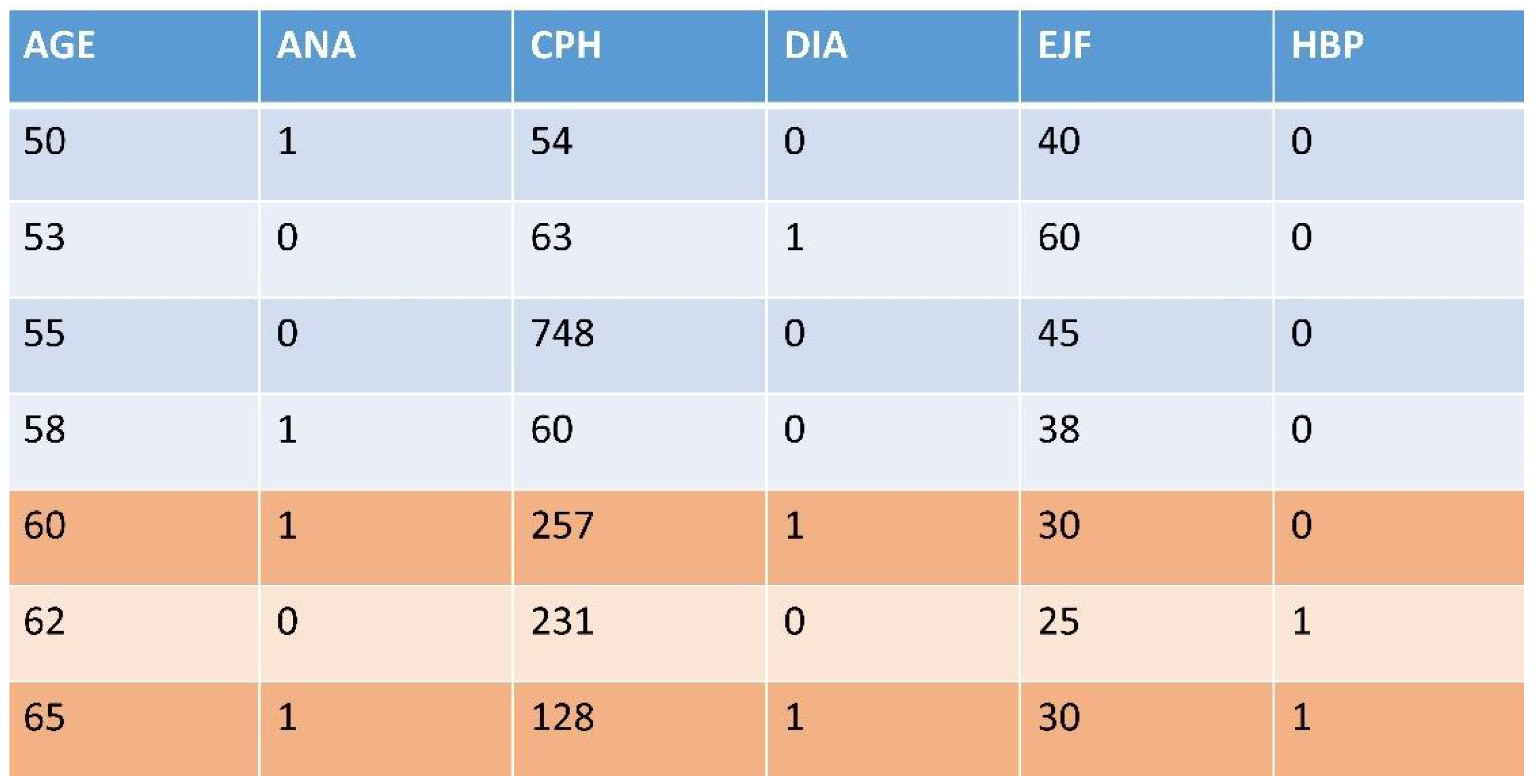
Figure 2.
The ordered lists of features of size 3 with the relative position of feature (3, 4, 6) on each list.
Figure 2.
The ordered lists of features of size 3 with the relative position of feature (3, 4, 6) on each list.
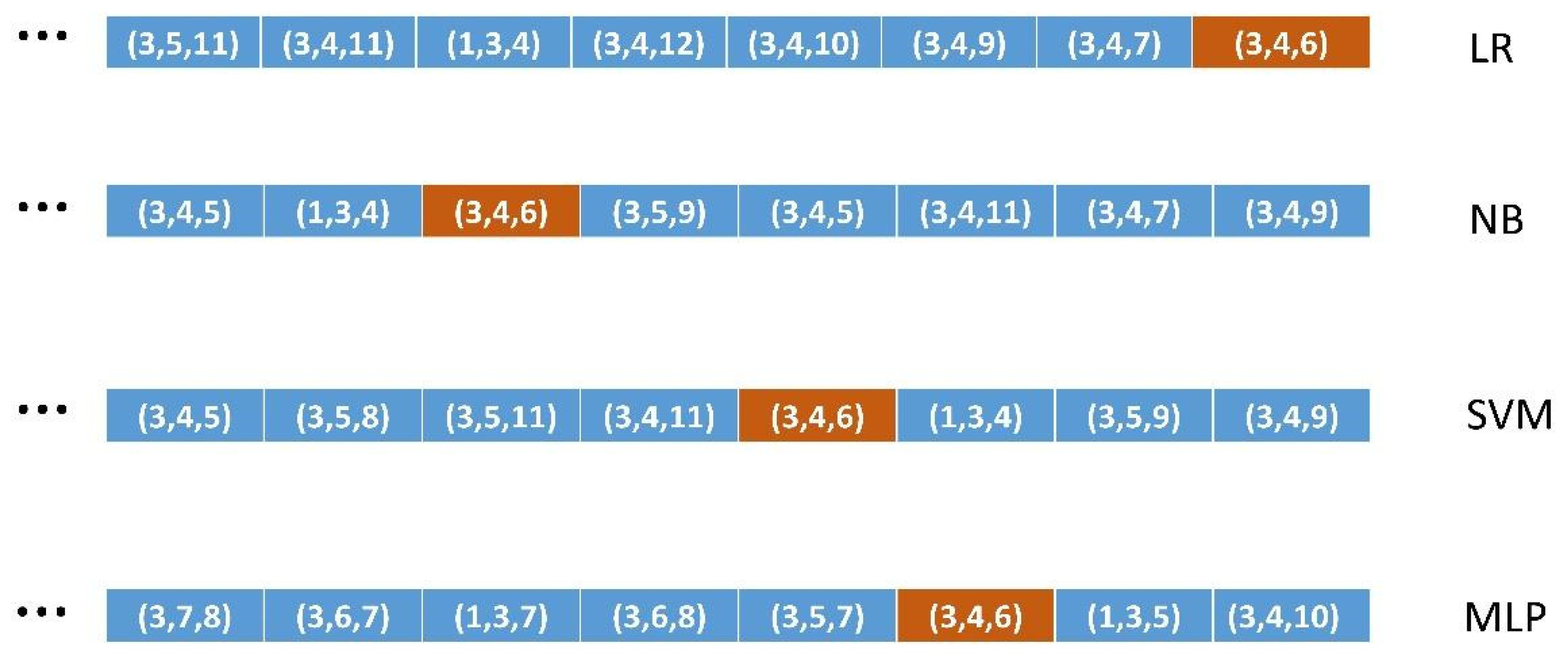
Figure 3.
Ordering of ML algorithms on each probability distribution.
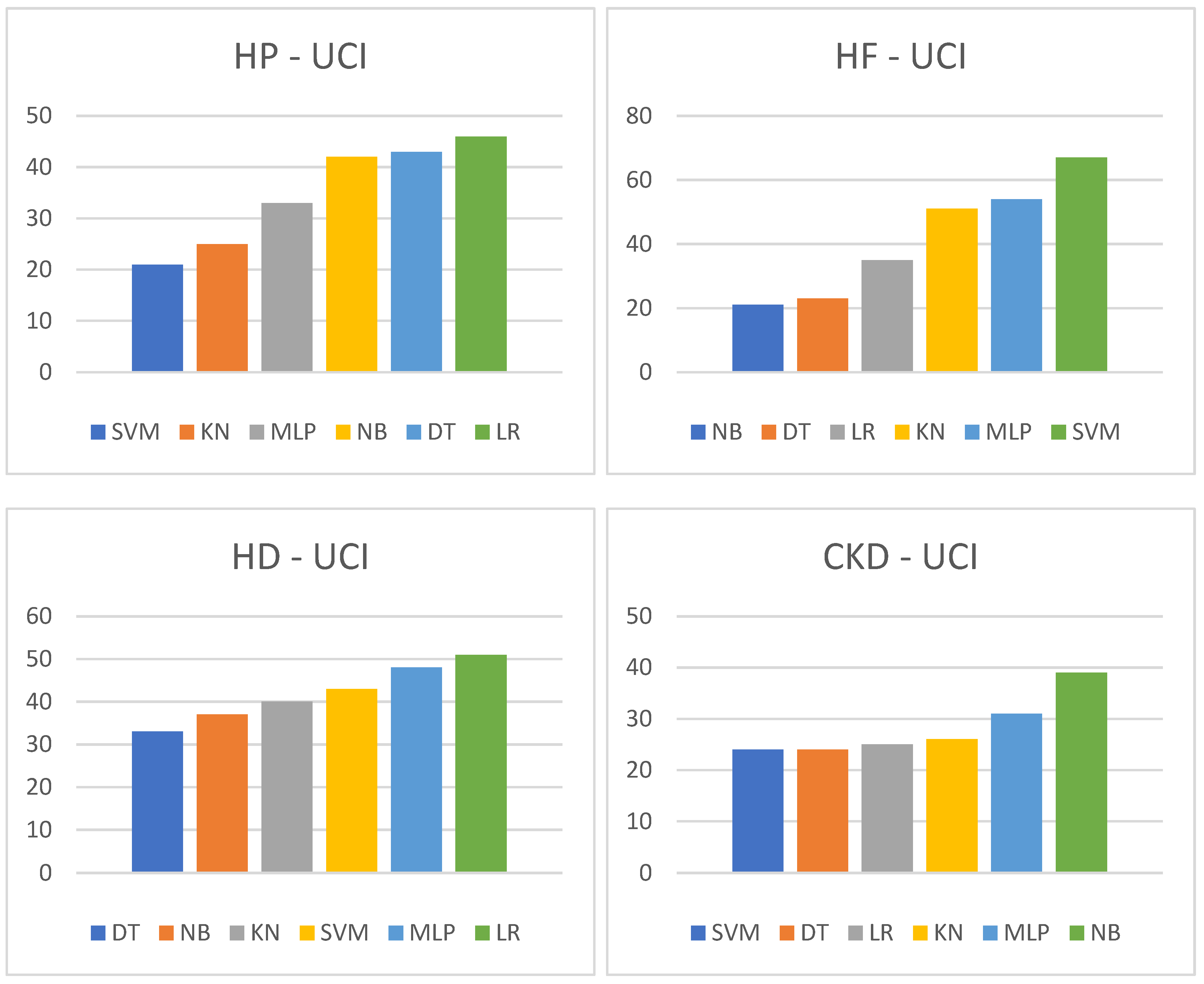
Table 1.
Dataset feature splitting.
|
Method 1. Dataset feature splitting Select a column (feature) from the set of features of the dataset Sort the dataset using that column Set a threshold in the ordered column Divide the dataset into two parts (higher and lower datasets) |
Table 2.
Ordered lists building.
|
Method 2. Ordered list building For each ML algorithm For each FS size 3 through 6 Compute the weighted F measure of the supervised ML execution Add it to the sorted list corresponding to each combination (ML algorithm, FS size) |
Table 3.
Codifying medical knowledge.
|
Method 3. Medical knowledge encoding For each working dataset generated using DFS having one driving feature Fi For each remaining feature in the dataset Fj Query a LLM to check if the pair (Fi, Fj) is medical knowledge relevant or not If yes, add Fj to the list of relevant features with respect to Fi |
Table 4.
Detail of Table 16 showing the list of features knowledge relevant with respect to the DFS-driving feature of the dataset. HP-UCI probability distribution. See Appendix 1 for the numbers of the features. .
Table 4.
Detail of Table 16 showing the list of features knowledge relevant with respect to the DFS-driving feature of the dataset. HP-UCI probability distribution. See Appendix 1 for the numbers of the features. .
| ALP H | (1,3,5,6,7,9,10,11,12) |
| CRE H | (1,4,5,6,12) |
Table 5.
ML algorithms relevance power.
|
Method 4. ML algorithms relevance power For each of the 6 ML algorithms For each working dataset and its driving medical feature Fi For each feature Fj in its list of medical knowledge relevant features For each of the 4 sizes F-measure-sorted lists Obtain and accumulate the position of Fj in the F-measure-sorted list Accumulate the positions of all the Fj for each size Return the ML algorithm with the maximum accumulated for each size |
Table 6.
Classification and knowledge relevance scores of the six ML algorithms for the case of the CRE H dataset corresponding to the Hepatitis C probability distribution.
Table 6.
Classification and knowledge relevance scores of the six ML algorithms for the case of the CRE H dataset corresponding to the Hepatitis C probability distribution.
| CRE H | ||||||
| size 3 | 161.8 (SVM) | 141.1 (LR) | 136.6 (MLP) | 135.0 (DT) | 134.8 (KN) | 132.0 (NB) |
| size 4 | 477.5 (SVM) | 432.4 (DT) | 412.9 (LR) | 406.6 (MLP) | 404.1 (NB) | 392.4 (KN) |
| size 5 | 942.2 (SVM) | 879.8 (DT) | 839.8 (MLP) | 819.6 (NB) | 815.5 (LR) | 787.4 (KN) |
| size 6 | 1299.4(SVM) | 1229.5 (DT) | 1174.3(MLP) | 1157.6 (NB) | 1144.8 (LR) | 1119.2 (KN) |
Table 7.
Detail of Table 17 showing the order of algorithms resulting in datasets ALP H and CRE H of the HP-UCI distribution. See Appendix 2 for the abbreviations of ML algorithms.
Table 7.
Detail of Table 17 showing the order of algorithms resulting in datasets ALP H and CRE H of the HP-UCI distribution. See Appendix 2 for the abbreviations of ML algorithms.
| ALP H | SVM,KN,MLP,DT,LR,NB |
| CRE H | SVM,DT,MLP,LR,NB,KN |
Table 8.
Detail of Table 18 in which we obtain an ordering of ML algorithms for the HP-UCI probability distribution. Lower scores mean better algorithms.
Table 8.
Detail of Table 18 in which we obtain an ordering of ML algorithms for the HP-UCI probability distribution. Lower scores mean better algorithms.
| SVM | KN | MLP | NB | DT | LR |
| 21 | 25 | 33 | 42 | 43 | 46 |
Table 9.
is a detail of Table 19 and shows the p-values returned by the KS test on two datasets of the HP-UCI distribution.
Table 9.
is a detail of Table 19 and shows the p-values returned by the KS test on two datasets of the HP-UCI distribution.
| ALP H | 1.1394834474e-05 |
| CRE H | 4.2769255669e-26 |
Table 10.
Six vectors of results of the averaged position in the ordered lists of each ML algorithm in the HP-UCI distribution with FS size three.
Table 10.
Six vectors of results of the averaged position in the ordered lists of each ML algorithm in the HP-UCI distribution with FS size three.
| HP-3 | AGE H | SEX H | SEX L | ALB L | ALP H | ALT H | BIL H | CHO H | CREH | PRO H |
| LR | 260.97 | 22.72 | 46.02 | 181.25 | 254.82 | 284.44 | 191.44 | 101.17 | 141.08 | 205.61 |
| NB | 267.32 | 26.46 | 46.17 | 182.02 | 248.15 | 263.85 | 203.93 | 130.34 | 132.04 | 205.65 |
| SVM | 267.09 | 31.51 | 46.24 | 188.25 | 261.16 | 275.26 | 217.63 | 138.53 | 161.76 | 208.95 |
| MLP | 262.86 | 23.11 | 49.42 | 181.16 | 251.13 | 273.78 | 201.84 | 132.26 | 136.59 | 206.89 |
| DT | 200.54 | 29.81 | 51.44 | 150.72 | 236.03 | 275.34 | 189.28 | 100.22 | 134.95 | 177.27 |
| KN | 270.33 | 29.71 | 46.17 | 187.93 | 257.04 | 280.88 | 210.11 | 139.65 | 134.83 | 216.31 |
Table 11.
P-values returned by the chi-squared test on the HP-UCI probability distribution.
| size 3 | size 4 | size 5 | size 6 | |
| HP | 0.0036986186 | 0.0009519294 | 0.0035663982 | 0.0187894355 |
Table 12.
Scores and ordering produced by the six ML algorithms on the HP-UCI dataset.
| HP-UC | ||||||
| size 3 | 213.0 (DT) | 209.3 (SVM) | 207.2 (KN) | 201.9 (LR) | 200.7 (MLP) | 199.0 (NB) |
| size 4 | 934.1 (SVM) | 928.8 (DT) | 925.0 (MLP) | 917.2 (KN) | 889.4 (LR) | 887.5 (NB) |
| size 5 | 2450.6 (SVM) | 2436.5 (DT) | 2413.9 (KN) | 2365.2 (MLP) | 2340.1 (NB) | 2335.2 (LR) |
| size 6 | 4218.5 (SVM) | 4206.7 (DT) | 4173.9 (KN) | 4058.8 (NB) | 4049.6 (MLP) | 4036.0 (LR) |
| Order | SVM | DT | KN | MLP | NB | LR |
Table 13.
Scores and ordering produced by the six ML algorithms on the HF-UCI dataset.
| HF-UC | ||||||
| size 3 | 268.9(DT) | 244.5 (KN) | 227.0 (NB) | 218.8 (SVM) | 211.9 (MLP) | 203.5 (LR) |
| size 4 | 1208.5(DT) | 1072.8 (KN) | 1022.9 (NB) | 1008.2 (SVM) | 968.1 (MLP) | 937.9 (LR) |
| size 5 | 3179.7 (DT) | 2776.2 (KN) | 2744.1 (SVM) | 2706.2(NB) | 2600.5 (MLP) | 2553.0 (LR) |
| size 6 | 5481.8(DT) | 4872.2 (SVM) | 4826.8(KN) | 4712.2(NB) | 4587.9 (MLP) | 4547.1 (LR) |
| Order | DT | KN | SVM | NB | MLP | LR |
Table 14.
Best classified FSs of each size in the best performing ML algorithms on the HP-UCI dataset.
Table 14.
Best classified FSs of each size in the best performing ML algorithms on the HP-UCI dataset.
| HP-UCI | SVM | DT | KN | MLP |
| FS size 3 | (5, 6, 10) | (5, 6, 12) | (5, 6, 7) | (3, 6, 7) |
| FS size 4 | (5, 6, 7, 10) | (4, 5, 6, 12) | (5, 6, 7, 10) | (6, 7, 10, 12) |
| FS size 5 | (4, 5, 6, 7, 10) | (5, 6, 7, 8, 12) | (4, 5, 6, 7, 10) | (4, 5, 6, 11, 12) |
| FS size 6 | (5, 6, 7, 9, 11, 12) | (1, 5, 6, 7, 8, 12) | (4, 5, 6, 7, 10, 11) | (4, 5, 6, 10, 11, 12) |
Table 15.
Best classified FSs of each size in the best performing ML algorithms on the HF-UCI dataset.
Table 15.
Best classified FSs of each size in the best performing ML algorithms on the HF-UCI dataset.
| HF-UCI | DT | KN | SVM | NB |
| FS size 3 | (5, 8, 11) | (5, 8, 9) | (4, 5, 12) | (1, 5, 12) |
| FS size 4 | (4, 5, 8, 11) | (2, 5, 8, 9) | (1, 5, 8, 10) | (2, 3, 5, 12) |
| FS size 5 | (2, 4, 5, 8, 11) | (2, 5, 8, 9, 11) | (1, 5, 7, 8, 10) | (2, 5, 8, 10, 12) |
| FS size 6 | (1, 3, 4, 5, 8, 11) | (2, 3, 5, 7, 8, 9) | (1, 5, 7, 8, 10, 11) | (1, 2, 5, 8, 9, 12) |
Disclaimer/Publisher’s Note: The statements, opinions and data contained in all publications are solely those of the individual author(s) and contributor(s) and not of MDPI and/or the editor(s). MDPI and/or the editor(s) disclaim responsibility for any injury to people or property resulting from any ideas, methods, instructions or products referred to in the content. |
© 2025 by the authors. Licensee MDPI, Basel, Switzerland. This article is an open access article distributed under the terms and conditions of the Creative Commons Attribution (CC BY) license (http://creativecommons.org/licenses/by/4.0/).
Copyright: This open access article is published under a Creative Commons CC BY 4.0 license, which permit the free download, distribution, and reuse, provided that the author and preprint are cited in any reuse.


