
Submitted:
11 April 2025
Posted:
11 April 2025
You are already at the latest version
Abstract
Accurate estimations of ETo is critical for hydrologic studies, efficient crop irrigation, water resources management and sustainable development. The evaluation of an empirical method for estimating hourly ETo, utilizing the incoming solar radiation and a relation between a function of relative humidity and vapor pressure deficit as an aerodynamic term was calibrated under semi arid conditions, and assessed against the ASCE PM (2005) method for hyper arid to sub humid climatic regimes in the State of California. For hyper arid climatic conditions, the empirical method underestimated and had R2 values from 0.88 to 0.95 and RMSE values from 0.062 to 0.115 mm h-1. Hyper arid climatic conditions, correspond to lower R2 and different relations between the VPD and the inverse of the natural logarithm of relative humidity (1/lnRH). For arid semi arid and sub humid climatic conditions the empirical method performed satisfactorily. The RMSE was calculated for various intervals of the range of the observed wind speed values and it was satisfactory for >99% of all data. The RMSE was also calculated for various intervals of the observed values of VPD and was satisfactory for >97% of all data except for hyper arid stations (59% of u2 and 60% of VPD data).
Keywords:
hyper arid
; arid
; semi arid
; reference evapotranspiration
; evaluation
; empirical relation
1. Introduction
Reference evapotranspiration is important for
efficient irrigation, conservation of water resources, mitigation of climate
change impacts, hydrologic studies etc. This importance is reflected in the
numerous models that have been proposed in the scientific literature.
Combination methods use a theoretical background [1–3] and need data, which are not always available,
to estimate evapotranspiration rates. The theoretical background of these
methods is a key component of their ability to predict evapotranspiration rates
with much higher accuracy, compared to other methods which lack such
background. Therefor they are applicable to many different climates and
altitudes. The PM method was evaluated [4]
against lysimeter data and using data from hyper arid, arid, semi arid,
subhumid, humid and high altitude climatic regimes, and concluded that they
were sufficiently accurate. ASCE PM (2005), [3]
standardized the calculations of the method so as the result of the
calculations, the reference evapotranspiration (ETo) rates, would be comparable
between researchers and is widely accepted from the scientific community.
Empirical methods are more easy to use and are more
flexible in the data they require [5–12].
Fewer input variables on the other hand, combined with the lack of a
theoretical background, lead to a narrowing of their ability to estimate with
accuracy. When applied to climatic regimes or locations other than those to
which they were calibrated, the error increases. The evaluation of a method at
a different climatic regime or location, should be carried out, before its
application. ASCE PM (2005) is the standard method against which empirical
methods are evaluated and can only yield reliable estimates under reference
conditions.
Many authors have evaluated empirical methods
against PM, [13–23] in order to determine the
reliability of these methods for purposes like irrigation scheduling,
hydrological sustainable development of natural resources, establishing trends
for ETo etc. Empirical methods have also been evaluated against measurements by
various researchers [24–27]. The evaluation of
these methods contribute to the establishment of a sustainable relationship
between human activities, i.e. agriculture and conservation of natural
resources. [28] investigated the driving
forces for the estimation of potential evapotranspiration (PET) in hyper arid
conditions of NW China using the Hargreaves Samani method [29] as PET’s driving forces are very important in
mitigating the impacts of climate change. [30] evaluated 20
different empirical models for the hyper arid climatic conditions of the State
of Qatar. Empirical models are subject to limitations and the investigation of
their accuracy is important for crop growth, water resources management etc. It
is important that the evaluations against PM methods should be in a reference
environment otherwise systematic cumulative errors occur [31].
Significant agricultural activity in California [32] and is variety of local climatic regimes [33] impose the need for an evaluation of the
methods that estimate evapotranspiration to asses their validity. Numerous
researchers have conducted studies that evaluate empirical methods that
estimate evapotranspiration for the State of California [34,35]. The network of agrometeorological stations
(CIMIS) provides data under reference environment which is necessary for the
evaluation of empirical methods against ASCE PM (2005) method.
[39] compared the
daily vs the hourly time step of the ASCE PM equation and suggested that the
efficiency of precision agriculture can benefit from hourly estimations of
reference ETo. There are a few empirical methods that estimate ETo on an hourly
basis. [40] proposed an empirical method that
estimates hourly rates of reference ETo under semiarid climatic conditions,
calibrated with CIMIS - Davis data and validated with CIMIS and AUA
agrometeorological station’s data. The empirical method does not require wind
speed or temperature data and therefor it is suitable for application when wind
speed and temperature data are missing or are questionable. The empirical
method uses a function of relative humidity as an aerodynamic related term
which is increasingly important when conditions become drier. It relies on
short wave radiation and relative humidity measurements to estimate hourly
rates, to avoid the overestimation (=(5-6% on average) of ETo rates due to the
inclusion of net radiation as an input, when daily sums are considered [41].
In this paper, we evaluate the empirical method for
hyper arid, arid, semi arid and sub humid locations in the state of California
and the contribution of the aerodynamic related term to the accuracy of the
method in drier climatic conditions than the calibration conditions.
2. Materials and Methods
As a reference method, the ASCE-PM (2005) [3] method for the hourly rate of ETo is used, for
short crop (12 cm) The following equation is used:
ΕΤο, reference evapotranspiration in mm
h-1, Rn, Net radiation flux density in Mj m-2
h-1, G, the soil heat flux density in Mj m-2 h-1,
u2, the average hourly wind speed at 2 meters in m s-1,
T, the average hourly temperature at 2 meters in oC, Cd,
0.24 for daytime 0.96 for nighttime, , the saturation vapor pressure of the atmosphere
at Ta in kPa, ea, the actual vapor pressure of the
atmosphere in kPa, , the slope of the saturation vapor pressure curve
in kPa oC-1, , the psychrometric constant in kPa oC-1,
λ, the latent heat of vaporization in MJ kg-1.
Hourly rate of ETo was also estimated with the [40] method, called the empirical method from now
on, The measured independent variables of the empirical equation are Rs (short
wave radiation) and RH (%). Theoretical daylight hours (N) is also a necessary
quantity and it is calculated from the location of the station (latitude) and
the time of the day of the year (julian day, 1-365). It takes into account the
daylight hours (N) as a fraction of the 24 h period (fN) e.g. a
daylight duration (N) of 12 hours would give an fN value of
12/24= 0.5.
The equation is
where, ETo the hourly rate of ETo in mm h-1,
Rs the incoming short wave (solar) radiation in W m-2, RH
the relative humidity %, fN a function of the the theoretical daylight
hours as a fraction of the total (24h), fNmin the minimum theoretical
daylight hours of the year as a fraction of the 24h.
Statistical and climatic indices
Coefficient of determination,
where, is the ASCE PM value, is its average, is the estimation of the empirical method, and is its average.
Slope. The slope of the regression line has
the following equation:
Same symbols as in equation (3).
Intercept.
The intersection of the regression line and Y axis:
Same symbols as above (3)
Root mean square error (RMSE).
Root mean square error is a weighted measure of the error with the same units as the dependent variable,
Same symbols as above.
[42] proposed a value of 0.073 mm h-1 as the upper limit for an acceptable estimation for the RMSE. This limit is used in this study as an optimum value for the performance of the empirical method. RMSE values up to ~ 90W m-2, or 0.13 mm h-1 for hourly values, were considered reasonable by other researchers [43]. This value is considered as the upper limit for the RMSE and for values between 0.073 mm h-1 and 0.13 mm h-1, further research is suggested.
Index of agreement (IoA).
According to this index, perfect agreement between the empirical method and ASCE (2005) correspond to 1, while total disagreement correspond to a value of zero. The IoA was introduced by [44].
symbols have the same meaning as above (3).
The Aridity Index (AI)
The Aridity Index (AI) is a climatic index used to assess the dryness of a geographical location (Kukal and Irmak, 2016). The AI was calculated as the ration of yearly values of precipitation (nominator,mm) and ETo (denominator, mm), according to the following equation:
Based on the value of the aridity index, dryness is classified to hyper-arid (AI≤0.05), arid (0.05<AI≤0.20), semi arid (0.20<AI≤0.50) and sub humid (0.50<AI≤0.75).
Data
CIMIS network
CIMIS stands for California Irrigation Management Information System. It is operated by the Water Use and Efficiency Branch of the Division of Statewide Integrated Water Management of the California Department of Water Resources (DWR). 145 active stations are operated with data collected every minute and stored and processed in the central computer of the CIMIS headquarters. Hourly data for e.g. 1300 h refer to the 60 minutes prior to 1300 (1200-1300).
Quality Control (QC) is performed for the collected data, which are then being flagged accordingly. Programmed calculations are stored along with the flagged data. Data access if free for the public, provided that the interested individuals are registered.
Values of RH below or equal to 4% were excluded (four records of Indio 2 station). All available monthly data of 139 stations were downloaded from the database, and summed to yearly values. 26364 records with monthly data in total were used. For each of the 139 stations of the CIMIS network, yearly averages were calculated, for reference evapotranspiration and for all the meteorological parameters. California is characterized by a wide variety of microclimates, [33]. The calculated averages from the 139 stations of the CIMIS network were used for the selection of stations representative of the observed variety of microclimates in the state of California. Based on these calculated averages, ten (10) CIMIS meteorological stations were selected (see Table 1). Years with complete records were preferred as much as possible. From the ten (10) CIMIS meteorological stations, six (6) were selected according to the value of the aridity index (AI) with values of the AI ranging from 0.00 to 0.74. The AI values of the stations chosen, cover the range of observed AI values, in a representative way. The AI for the Davis station of the CIMIS network was calculated equal to 0.33 for the whole period of its operation (1982-Apr 2015).
Four (4) CIMIS meteorological stations were selected according to maximum average VPD value (vapor pressure deficit of the atmosphere, 2.3 kPa average value for Cadiz station, Stn Id 221), maximum average u2 value (wind speed at 2 meters above ground surface, 3.4 m s-1 average wind speed value for Twitchel Island station, Stn Id 140), maximum average ETo value (1838 mm year-1 average value for Seeley station, Stn Id 68) and maximum average air temperature value (23.1 oC average air temperature value for Oasis station, Stn Id 136). 83807 hourly records were downloaded in total for all ten stations.
3. Results and Discussion
83807 hourly records from 10 stations of the CIMIS network were used to evaluate the estimations of an empirical method for hyper arid, arid, semi arid and subhumid climatic conditions, for the state of California.
The hourly rate of ETo was calculated (83807 values) with the empirical method. The CIMIS values of the hourly rate of ETo according to the ASCE PM (2005) method, were used. Yearly totals of hourly ETo estimates were calculated for both the empirical and the ASCE PM (2005) method. Additionally, the absolute difference between the two methods (Empirical total – ASCE PM total), the relative difference expressed as a percentage of the ASCE PM (2005) yearly total, and four statistical indicators (R², RMSE, slope, and IoA) were computed (see Table 2).
The values (83807) calculated with the empirical method and those calculated with the ASCE PM (2005) method, were summed as seen in the last row of Table 2. The sum of the empirical method was 15486.6 mm while the ASCE PM (2005) had a sum of 15733.7 mm for all the 10 stations we used for evaluation. The difference was found equal to -247.1 mm or -1.6% of the sum of the estimations of the ASCE PM (2005) method for all the 10 stations. In Figure 1 we can see the cumulative plot of the hourly values of both methods. The statistical indices for the 83807 hourly estimations of both methods were also calculated. The coefficient of determination (R2) was found equal to 0.95, the RMSE was found equal to 0.060 mm h-1, the slope of the regression line between the values of the hourly ETo estimations of the empirical method and the values of the hourly ETo estimations of the ASCE PM (2005) method was found equal to 0.88. The IoA was found equal to 0.978. The value of the RMSE is satisfactory. The agreement between the two methods was found satisfactory.
3.1. Stations with Hyper-Arid Climatic Regimes
Four CIMIS stations (all located in the southern and most arid part of California and characterized by similar climatic conditions), out of the 10 used for this study, were characterized by hyper arid conditions. Indio 2 had AI=0.00, Cadiz Valley had AI=0.03 and the highest yearly average VPD value, Seeley had AI=0.04 and the highest annual ETo value, Oasis had AI=0.03 and the highest annual average temperature. We examined the four stations as a group because these four represent the most arid part of California.
The sum of the values estimated with both the empirical method and the ASCE PM (2005) method were in good agreement for all the four stations. Indio 2 had the highest underestimation with 9.6% and the minimum underestimation was observed for Oasis station with 0.4%. The minimum R2 value was observed for Cadiz Valley station with 0.88 while Oasis station had the best R2 value with 0.95 (see Figure 2). Oasis station had the minimum RMSE value 0.062 mm/h) between the two methods. The maximum value for RMSE for the hyper arid stations was observed at Cadiz Valley station equal to 0.115 mm/h. The slopes of the regression lines between the two methods (see Figure 2) were all below 1, showing a consistent underestimation, with Cadiz Valley station having the minimum value equal to 0.60. The maximum value of the slope of the regression line is for the Oasis station, equal to 0.85, again indicating underestimation on the part of the empirical method. The values of the IoA ranged from 0.919 for the Cadiz Valley station and 0.983 for the Oasis station.
While the value of IoA and the yearly totals of the values of the two methods, for the four hyper arid stations of the CIMIS network, indicate a good agreement, the values of the slope of the regression lines are small and the RMSE values although smaller than 0.13 mm h-1, are the highest, in comparison with all the other stations, and with the exception of Oasis are not satisfactory. Radiation methods perform well in humid climates, [47,48], and tend to underestimate in arid climates, [48]. The main reason for this is that the higher temperatures and lower moisture content of the atmosphere, increase the significance of the aerodynamic term of the PM method in hyper arid climates compared to more humid climates. Vapor pressure deficit (VPD) and wind speed (u2) are the two important factors of the aerodynamic term of the PM method which determine the performance of radiation methods in hyper arid climates.
Since the inputs of the empirical method does not include u2, therefor, its coefficients reflect the observed values of u2 during calibration (Davis, 2000, average u2 value 2.52 m s-1). Higher observed u2 values in the four hyper arid stations, would contribute to an underestimation of the hourly ETo values. In the same way lower observed u2 values in the four hyper arid stations, would contribute to an overestimation of the hourly ETo values. The average hourly values of wind speed for the three hyper-arid stations (Indio 2, Seeley, Oasis) are lower than the average hourly value of wind speed for Davis, year 2000 (2.52 m s-1) and one station (Cadiz) has a higher yearly average wind speed (2.73 m s-1). Cadiz station’s yearly sum of the hourly estimations of the empirical method was very close (-1.6%) to that of the ASCE PM (2005) yearly sum. The biggest underestimation was for Indio 2 station which had an average hourly wind speed value lower (2.33 m s-1) than that for Davis station (2.52 m s-1). [49] found that ETo is least sensitive in u2. [50] argued that combination methods are less sensitive to u2. The findings of this research agree with [49,50].
3.1.1. Investigation of the VPD—1/ln(RH) Relation
We calculated the values of slope, Intercept and R2 for all the hourly records of the four stations (8235 for Indio 2, 8741 for Cadiz, 7679 for Seeley and 7903 for Oasis), for the hourly records of the warm part of the year (80<DOY<267) for each station and for all the hourly values of the warm part of the year of the four stations (80<DOY<267, 15011 records), for the hourly records of the cold part of the year (remaining part of the year) for each of the four stations and for the all the values of the cold part of the year of the four stations (17547 records, see Table 3).
The calculated R2 values, ranged from 0.45 (Seeley station, All hourly values) to 0.80 (Oasis station, cold period). The R2 value for all the hourly values (32558) was found equal to 0.52. For both the warm (80<DOY<267) and the cold period (remaining part of the year) R2 was calculated equal to 0.54. Slope values ranged from 0.0175 (Seeley station, all hourly values) to 0.0359 (Cadiz station, cold period). Smaller slope values were calculated for the warm part of the year and higher values of the slope were calculated for the remaining (cold) part of the year. During the cold part of the year the range of VPD is smaller while the range of RH is not affected as much. Intercept values ranged from 0.2205 (Oasis station, cold period) to 0.2671 (Cadiz station, all hourly values).
For saturated atmospheric conditions (VPD=0) the 1/ln(RH) term takes its minimum value (0.2174). As VPD values increase so does the value of the 1/ln(RH) term, giving higher values for the intercept of the regression line between VPD and 1/ln(RH). The maximum intercept value is for Cadiz station (intercept=0.2671) which also has the highest average yearly VPD value compared to the other three stations (and also to all of the 10 CIMIS stations used for this study). The minimum intercept value is for Oasis station (intercept=0.2205) which also has the lowest average yearly VPD value of the four (drier) stations (see Table 3).
Values of R2 were much higher when grouped on a daily basis. On a daily basis, values of actual vapor pressure is more or less the same, [51], so the change of the VPD is due to the change of air temperature which determines the saturation vapor pressure of the atmosphere. RH then, follows the change of air temperature [48].
We investigated the assumption, that actual vapor pressure of the atmosphere during the day, remains more or less constant as [51], suggested. We examined the calculated R2 values for all the four arid stations (Indio 2, Cadiz, Seeley, Oasis) and found that Indio 2 station had 63 days with R2 less than 0.90, Cadiz station had 146 days with R2 less than 0.90, Seeley station had 118 days with R2 less than 0.90 and Oasis station had 31 days with R2 less than 0.90. The same calculation for Davis station gave two days with R2 less than 0.90 . During those two days we had abrupt changes in weather patterns which gave big shifts in the values of the actual vapor pressure.
We used 24 hourly records of DOY 97, year 2008, from Indio 2, to calculate the R2 between the values of VPD and the values of the inverse of the natural logarithm of RH. When we used the average of the 24 observed actual vapor pressure values for that day (DOY 97) for the Indio 2 station, equal to 0.91 kPa, to calculate the vapor pressure deficit and the RH, the R2 value was found equal to 1. We repeated the calculation using the observed 24 hourly values of the actual vapor pressure and we found R2 equal to 0.18.
During that day a continuous supply of moisture to the atmosphere was recorded, as shown by the rising curve of actual vapor pressure in Figure 2, until approximately 0800 to 0900 in the morning. The value of the actual vapor pressure was equal to about 1.05 kPa for the rest of the day. After 1800 hour when actual vapor pressure reached a daily minimum, it continued to increase until the end of the day (2400 h). Increases of air humidity during the night are not normally associated with evapotranspiration. Evapotranspiration during the night have been reported by [52] and was associated with wind speeds greater than 6 m s-1 at 3 m above ground, as the wind is the only turbulence source during the night. During DOY 97, year 2008, for Indio 2 station, the mean wind speed was calculated from the hourly values of wind speed and found equal to 4.6 m s-1 at 2 m above ground which equals 4.99 m s-1 at 3 m above ground. The conversion of the wind speed from 2 m to 3 m was made in accordance with the guidelines given by [48]. Therefore, the diurnal pattern of air temperature only partly accounts for the variation of the vapor pressure deficit of the atmosphere in such cases. As the diurnal variation of the actual vapor pressure, gets larger, it reduces the R2 value between the vapor pressure deficit of the atmosphere and the inverse of the natural logarithm of the RH of the atmosphere. As a result, the model estimates a smaller portion of the variation of the dependent variable, which results in reduced accuracy of the estimations of the empirical method.
Figure 3.
Plot of the actual vapor pressure (kPa, left vertical axis, triangles) and of the air temperature (oC, right vertical axis, squares) for Julian Day 97, year 2008, for Indio 2 station of the CIMIS network. In the x (horizontal) axis are the 24 hours of that day.
Figure 3.
Plot of the actual vapor pressure (kPa, left vertical axis, triangles) and of the air temperature (oC, right vertical axis, squares) for Julian Day 97, year 2008, for Indio 2 station of the CIMIS network. In the x (horizontal) axis are the 24 hours of that day.

The empirical method uses 1/ln(RH) to introduce the aerodynamic contribution to ETo. As we climatic conditions change from semi arid to hyper arid, the empirical method adapts satisfactorily. The term contributes to this behavior despite the different climatic regime under which it was calibrated. Hyper arid climatic conditions are the most dry so we investigated arid, semi arid and also, for completeness of the research, subhumid conditions.
3.2. Stations with Arid, Semi Arid and Sub Humid Climatic Regimes
From the remaining six out of the ten CIMIS stations selected, two are classified as arid (Five Points station, 8759 records, AI=0.10, Fresno station, 8783 records, AI=0.20), three are classified as semi arid (Colusa station, AI=0.34, 8254 records, Durham station, AI=0.45, 8664 records, Twitchel island station, AI=0.23, 8318 records, also the station with the highest wind speed value) and one sub humid station (Santa Rosa station, AI=0.74, 8471 records).
We calculated the values of the hourly ETo estimations of the empirical method for all the 51249 hourly records of the six CIMIS stations, and we compared them with the values of the hourly ETo estimations of the ASCE PM (2005). The sum of the values of the empirical method for all the six stations, was found equal to 7925.9 mm and it overestimated the ASCE PM (2005) totals, equal to 7900.3, by 25.6 mm or 0.32%. The average difference of the total of the empirical method for each station from the ASCE PM (2005) totals sum of the values of the hourly ETo estimations of the ASCE PM (2005) method was equal to 4.1 mm per year. The overestimation of the empirical method was small and acceptable for the sum of the values for all the six stations (51249 hourly records).
We also compared the sum of the values for each station. The empirical method overestimated in three stations (Five Points, Durham, Santa Rosa) with overestimations ranging from 22.6 mm to 126.8 mm, and underestimated in the remaining stations (Fresno, Colusa, Twitchel Island) with underestimations ranging from 33.6 mm to 66.0 mm. Both underestimations and overestimations were observed to arid and semi arid stations. The over or under estimations between the two methods, could not be attributed to the climatic regime of the stations when the yearly sum of the hourly ETo estimations of the two methods were compared. The differences were small and were considered satisfactory.
We calculated R2 between the values of the two methods for each station (see Table 2, Figure 4). The R2 ranged from 0.96 (Five Points station, arid) to 0.98 (Santa Rosa station, sub humid) and were considered satisfactory, the RMSE values showed a minimum of 0.033 mm h-1 (Santa Rosa station, sub humid) and a maximum of 0.046 mm h-1 (Five Points, arid). All RMSE values were below the threshold of 0.073 mm h-1 set by [42]. The RMSE values calculated were small and satisfactory for the empirical method. The slope of the regression lines between the two methods for the remaining stations were calculated (see Figure 4, Table 2).
The minimum slope value of the regression line was equal to 0.90 (Five Points station, arid) and the maximum value was equal to 1.11 (Santa Rosa station, subhumid). These values however were not reflected on the annual totals for the two methods, which were almost identical. The scatterplots of the estimations of the two methods confirm the agreement between the two methods. The IoA was also calculated for the two methods. The maximum value of the IoA was equal to 0.993 (Fresno station, arid and Colusa station, semi arid) and the minimum value of the IoA was equal to 0.989 (Five Points station, arid). The IoA values calculated for the estimations of the two methods were satisfactory.
We plotted (see Figure 5), the hourly values of the two methods, for DOYs 170-175 (19 June until 24 June) for four stations with arid (Five Points, Fresno) and hyper arid (Indio 2, Oasis) climatic conditions. The plotted values showed a good agreement for the arid stations and an underestimation for the hyper arid station of Indio 2, Oasis station (hyper arid) is more satisfactory.
3.3. Evaluation of Relation of the Values of u2 and VPD, and the RMSE Values Between the Two Methods, for All the Climatic Regimes
The accuracy of the estimations was investigated in relation to the aerodynamic term related variables (wind speed, VPD) because of their significance to dry climatic conditions. The range of the observed values (83807 hourly values for each parameter) was equal to 0-14.8 m s-1 for the wind speed and 0-9.23 kPa for the VPD. Wind speed and VPD values were grouped into intervals of 1 m s-1 for u2, and of 1 kPa for the VPD. RMSE was calculated for the respective values of the two methods, that correspond to each group of u2 and VPD. Intervals different from 1 m s-1 or 1 kPa were introduced when the RMSE was approaching the limits of 0.073 mm h-1 as suggested by [42] or 0.13 mm h-1 set by [43]. We repeated this procedure for the hourly values of the hyper-arid stations (Indio 2, Cadiz, Oasis, Seeley, 32558 records) for the hourly values of the arid stations (Five Points, Fresno, 17542 hourly records), for the hourly values of the semi arid stations (Colusa, Durham, Twitchel island, Santa Yanez, 34010 hourly records) and for the hourly values of the sub humid station (Santa Rosa, 8471 hourly records). We then calculated the percentage of the estimations that yield RMSE values lower than 0.073 mm h-1 and lower than 0.13 mm h-1 (see Table 4) for each variable and for each climatic regime.
The RMSE of the estimations of the two methods, was below 0.073 mm h-1 [42], for the 94% of the hourly ETo estimations and 99% was below 0.13 mm h-1 [43], when we examined all the hourly records (83807 records). The RMSE of the two methods is in almost all cases below the 0.073 mm h-1 limit for the 97-100% for arid, semi arid and sub humid climatic regimes for both the wind speed and the VPD. For all the previous climatic regimes the empirical method had satisfactory RMSE values.
Approximately 60% of the empirical method’s estimations, had RMSE values smaller than 0.073 mm h-1 86-94% of the estimations had RMSE smaller than 0.13 mm h-1 in the case of the hyper-arid stations (32558 hourly records). The performance of the empirical method for the hyper-arid stations was not satisfactory. Further research of the uncertainty of the aerodynamic related term for hyper-arid climatic conditions is needed.
4. Conclusions
The empirical method [40] was evaluated, for hyper-arid, arid, semi arid, sub humid, against the ASCE PM (2005) method using four statistical indices (RMSE, R2, slope, IoA). CIMIS database provided all the data (83807 records) used for this study. Ten 10 stations were selected based on their climatic regime and the values of meteorological parameters related to the aerodynamic term of the PM equation. The RMSE value of 0.073 mm h-1 was set a threshold for the evaluation of the method.
The statistical indices for all the 83807 hourly values of the two methods were satisfactory. The empirical method overestimated the sum compared to ASCE PM (2005) by 3.2%. RMSE value was satisfactory and below the limit of 0.073 mm h-1.
In the four most arid stations (min AI value, maximum VPD, maximum ETo, maximum temperature), the empirical method showed the highest RMSE values (0.062 mm h-1 to 0.115 mm h-1), the smallest slope values and consistent underestimation for all four stations. The relation of VPD and 1/ln(RH) which the empirical method takes into account, was investigated. The VPD - 1/ln(RH) relation, utilized by the empirical method, reflects the semi arid climatic conditions, under which it was calibrated. Very arid climatic conditions correspond to different VPD - 1/ln(RH) relations. Varying moisture content of the atmosphere during the day reduce the coefficient of determination between VPD and 1/ln(RH) therefor reduce the accuracy of the empirical method. Low values of the coefficient of determination between the two variables were observed in hyper-arid conditions. Further research is recommended for hyper-arid climatic conditions. The performance for semi arid climatic conditions was satisfactory as expected. RMSE values were 0.037 mm h-1 and 0.041 mm h-1. The uncertainty related to arid climatic conditions was satisfactory (RMSE 0.038-0.046). Both RMSE values were below the 0.073 mm h-1.
The aerodynamic term of the method contributes to the adaptation to climatic conditions much drier than originally calibrated for and is adequate for ETo assessments within the limits set for the examined data. For extremely dry conditions a recalibration of the equation would be recommended. Evaluation of the empirical method for other locations with similar climatic regimes is recommended.
Funding
This research received no external funding.
Institutional Review Board Statement
Not applicable.
Informed Consent Statement
Not applicable.
Data Availability Statement
Data are freely available from CIMIS. Registration of user is required for downloading the desired data. The author can provide the data upon request.
Acknowledgments
The author of the manuscript are grateful to all those who maintain the CIMIS network and generously provide the gathered data free to the scientific community. Without their contribution this paper would not have been possible to accomplish.
Conflicts of Interest
The author declare no conflict of interest.
References
- J. L. Monteith, Evaporation Monteith65.pdf, Symposium. Academic Press, Inc., NY., 1965.
- H. L. Penman, “Natural Evaporation from Open Water, Bare Soil and Grass,” Proc. R. Soc. A Math. Phys. Eng. Sci., vol. 193, no. 1032, pp. 120–145, Apr. 1948.
- Walter et al., “The ASCE Standardized Reference Evapotranspiration Equation,” in Standardization of Reference Evapotranspiration Task Committee Final Rep. ASCE, Reston, VA., 2005.
- M. Jensen, R. Burman, and R. G. Allen, “Evapotranspiration and irrigation water requirements,” 1990.
- S. Alexandris, P. Kerkides, and A. Liakatas, “Daily reference evapotranspiration estimates by the ‘Copais’ approach,” Agric. Water Manag., vol. 82, no. 3, pp. 371–386, Apr. 2006.
- S. Alexandris and P. Kerkides, “New empirical formula for hourly estimations of reference evapotranspiration,” Agric. Water Manag., vol. 60, no. 3, pp. 157–180, May 2003. [CrossRef]
- H. F. Blaney, W. D. Criddle, B. H., and C. W., “DETERMINING WATER REQUIREMENTS in IRRIGATED AREAS from CLIMATOLOGICAL and IRRIGATION DATA,” Washington D.C., 1950.
- E. T. Linacre, “A simple formula for estimating evaporation rates in various climates, using temperature data alone,” Agric. Meteorol., vol. 18, no. 6, pp. 409–424, Dec. 1977.
- G. F. Makkink, “Testing the Penman formula by means of lysimeters,” J. Inst. Water Eng., vol. 11, no. 3, pp. 277–288, 1957.
- C. H. B. Priestley and R. J. Taylor, “On the Assessment of Surface Heat Flux and Evaporation Using Large-Scale Parameters,” Mon. Weather Rev., vol. 100, no. 2, pp. 81–92, Feb. 1972.
- C. W. Thornthwaite, “An approach towards a rational calssification of climate,” Geogr. Rev., vol. 38, no. 1, pp. 55–94, 1948. [CrossRef]
- D. E. Tsesmelis, I. Machairas, N. Skondras, P. Oikonomou, and P. E. Barouchas, “GAIA: A New Formula for Reference Evapotranspiration,” Atmosphere (Basel)., vol. 15, no. 12, p. 1465, Dec. 2024. [CrossRef]
- P. Paredes, L. S. Pereira, J. Almorox, and H. Darouich, “Reference grass evapotranspiration with reduced data sets: Parameterization of the FAO Penman-Monteith temperature approach and the Hargeaves-Samani equation using local climatic variables,” Agric. Water Manag., vol. 240, p. 106210, Oct. 2020. [CrossRef]
- S. Alexandris, R. Stricevic, and S. Petkovic, “Comparative analysis of reference evapotranspiration from the surface of rainfed grass in central Serbia , calculated by six empirical methods against the Penman-Monteith formula,” Eur. Water, pp. 17–28, 2008.
- C. Chatzithomas, “Evaluation of a radiation-based empirical model for estimating hourly reference evapotranspiration for high-altitude climatic conditions: A case study for the state of California,” J. Earth Syst. Sci., vol. 128, no. 4, p. 79, Jun. 2019.
- S. Er-Raki et al., “Assessment of reference evapotranspiration methods in semi-arid regions: Can weather forecast data be used as alternate of ground meteorological parameters?,” J. Arid Environ., vol. 74, no. 12, pp. 1587–1596, Dec. 2010. [CrossRef]
- Z. Huo, X. Dai, S. Feng, S. Kang, and G. Huang, “Effect of climate change on reference evapotranspiration and aridity index in arid region of China,” J. Hydrol., vol. 492, pp. 24–34, 2013. [CrossRef]
- D. Itenfisu, R. L. Elliott, R. G. Allen, and I. A. Walter, “Comparison of Reference Evapotranspiration Calculations as Part of the ASCE Standardization Effort,” J. Irrig. Drain. Eng., vol. 129, no. December, pp. 440–448, 2003. [CrossRef]
- Raza et al., “Comparative Assessment of Reference Evapotranspiration Estimation Using Conventional Method and Machine Learning Algorithms in Four Climatic Regions,” Pure Appl. Geophys., vol. 177, no. 9, pp. 4479–4508, Sep. 2020. [CrossRef]
- G. Chipula et al., “Development and evaluation of site-specific evapotranspiration models in Malawi through a comparative analysis of existing models,” Phys. Chem. Earth, Parts A/B/C, vol. 137, p. 103814, Feb. 2025. [CrossRef]
- Eludire et al., “Evaluation of Evapotranspiration Prediction for Cassava Crop Using Artificial Neural Network Models and Empirical Models over Cross River Basin in Nigeria,” Water, vol. 17, no. 1, p. 87, Jan. 2025. [CrossRef]
- N. G. Cutting, S. Kaur, M. C. Singh, N. Sharma, and A. Mishra, “Estimating Crop Evapotranspiration in Data-Scare Regions: A Comparative Analysis of Eddy Covariance, Empirical and Remote-Sensing Approaches,” Water Conserv. Sci. Eng., vol. 9, no. 2, p. 65, Dec. 2024.
- S. Celestin, F. Qi, R. Li, T. Yu, and W. Cheng, “Evaluation of 32 Simple Equations against the Penman–Monteith Method to Estimate the Reference Evapotranspiration in the Hexi Corridor, Northwest China,” Water, vol. 12, no. 10, p. 2772, Oct. 2020. [CrossRef]
- G. Gao, X. Zhang, T. Yu, and B. Liu, “Comparison of three evapotranspiration models with eddy covariance measurements for a Populus euphratica Oliv. forest in an arid region of northwestern China,” J. Arid Land, vol. 8, no. 1, pp. 146–156, Feb. 2016.
- L. Zhao and W. Zhao, “Evapotranspiration of an oasis-desert transition zone in the middle stream of Heihe River, Northwest China,” J. Arid Land, vol. 6, no. 5, pp. 529–539, Oct. 2014.
- P. E. Ratshiedana, M. A. M. Abd Elbasit, E. Adam, and J. G. Chirima, “Evaluation of Micrometeorological Models for Estimating Crop Evapotranspiration Using a Smart Field Weighing Lysimeter,” Water, vol. 17, no. 2, p. 187, Jan. 2025. [CrossRef]
- M. R. Boso, F. S. Campos, and A. D. Pai, “Calibrated models to estimate Referensce evapotranspiration, for the city of Botucatu/Sp, in relation to the weighing lysimeter,” Model. Earth Syst. Environ., vol. 10, no. 6, pp. 6599–6612, Dec. 2024.
- Y. Lu et al., “Spatiotemporal Changes in and Driving Factors of Potential Evapotranspiration in a Hyper-Arid Locale in the Hami Region, China,” Atmosphere (Basel)., vol. 15, no. 1, p. 136, Jan. 2024. [CrossRef]
- G. H. Hargreaves and Z. Samani, “Reference crop evapotranspiration from ambient air temperature,” Am. Soc. Agric. Eng., no. 85, 1985.
- Ghiat, R. Govindan, and T. Al-Ansari, “Evaluation of evapotranspiration models for cucumbers grown under CO2 enriched and HVAC driven greenhouses: A step towards precision irrigation in hyper-arid regions,” Front. Sustain. Food Syst., vol. 7, 2023. [CrossRef]
- S. Alexandris and N. Proutsos, “How significant is the effect of the surface characteristics on the Reference Evapotranspiration estimates?,” Agric. Water Manag., vol. 237, p. 106181, Jul. 2020. [CrossRef]
- C. C. Faunt, M. Sneed, J. Traum, and J. T. Brandt, “Water availability and land subsidence in the Central Valley, California, USA,” Hydrogeol. J., vol. 24, no. 3, pp. 675–684, May 2016.
- B. Temesgen, S. Eching, B. Davidoff, and K. Frame, “Comparison of Some Reference Evapotranspiration Equations for California,” J. Irrig. Drain. Eng., vol. 131, no. 1, pp. 73–84, Feb. 2005. [CrossRef]
- R. L. Snyder, M. Orang, S. Matyac, and M. E. Grismer, “Simplified Estimation of Reference Evapotranspiration from Pan Evaporation Data in California,” J. Irrig. Drain. Eng., vol. 131, no. 3, pp. 249–253, Jun. 2005. [CrossRef]
- G. H. Hargreaves and R. G. Allen, “History and Evaluation of Hargreaves Evapotranspiration Equation,” J. Irrig. Drain. Eng., vol. 129, no. 1, pp. 53–63, Feb. 2003. [CrossRef]
- M. Gabriela Arellano and S. Irmak, “Reference (Potential) Evapotranspiration. I: Comparison of Temperature, Radiation, and Combination-Based Energy Balance Equations in Humid, Subhumid, Arid, Semiarid, and Mediterranean-Type Climates,” J. Irrig. Drain. Eng., p. 04015065, Dec. 2015. [CrossRef]
- J. Mutziger, C. M. Burt, D. J. Howes, and R. G. Allen, “Comparison of Measured and FAO-56 Modeled Evaporation from Bare Soil,” J. Irrig. Drain. Eng., vol. 131, no. 1, pp. 59–72, Feb. 2005. [CrossRef]
- S. Trajkovic, “Testing hourly reference evapotranspiration approaches using lysimeter measurements in a semiarid climate,” Hydrol. Res., vol. 41, no. 1, p. 38, Feb. 2010. [CrossRef]
- K. Djaman, S. Irmak, M. Sall, A. Sow, and I. Kabenge, “Comparison of sum-of-hourly and daily time step standardized ASCE Penman-Monteith reference evapotranspiration,” Theor. Appl. Climatol., vol. 134, no. 1–2, pp. 533–543, Oct. 2018. [CrossRef]
- C. D. Chatzithomas and S. Alexandris, “Solar radiation and relative humidity based, empirical method, to estimate hourly reference evapotranspiration,” Agric. Water Manag., vol. 152, pp. 188–197, Apr. 2015. [CrossRef]
- J. M. Blonquist, R. G. Allen, and B. Bugbee, “An evaluation of the net radiation sub-model in the ASCE standardized reference evapotranspiration equation: Implications for evapotranspiration prediction,” Agric. Water Manag., vol. 97, no. 7, pp. 1026–1038, Jul. 2010. [CrossRef]
- F. Ventura, D. Spano, P. Duce, and R. L. Snyder, “An evaluation of common evapotranspiration equations,” Irrig. Sci., vol. 18, no. 4, pp. 163–170, May 1999. [CrossRef]
- M. Choi, W. P. Kustas, and R. L. Ray, “Evapotranspiration models of different complexity for multiple land cover types,” Hydrol. Process., vol. 26, no. 19, pp. 2962–2972, Sep. 2012. [CrossRef]
- C. J. Willmott, “Some Comments on the Evaluation of Model Performance,” Bull. Am. Meteorol. Soc., vol. 63, no. 11, pp. 1309–1313, Nov. 1982.
- M. Kukal and S. Irmak, “Long-term patterns of air temperatures, daily temperature range, precipitation, grass-reference evapotranspiration and aridity index in the USA Great Plains: Part I. Spatial trends,” J. Hydrol., vol. 542, pp. 953–977, Nov. 2016.
- N. Shan et al., “Trends in potential evapotranspiration from 1960 to 2013 for a desertification-prone region of China,” Int. J. Climatol., vol. 36, no. 10, pp. 3434–3445, Aug. 2016. [CrossRef]
- J. Lu, G. Sun, S. G. McNulty, and D. M. Amatya, “A COMPARISON OF SIX POTENTIAL EVAPOTRANSPIRATION METHODS FOR REGIONAL USE IN THE SOUTHEASTERN UNITED STATES,” J. Am. Water Resour. Assoc., vol. 41, no. 3, pp. 621–633, Jun. 2005. [CrossRef]
- R. G. Allen, L. S. Pereira, D. Raes, and M. Smith, Crop evapotranspiration-Guidelines for computing crop water requirements-FAO Irrigation and drainage paper 56. Rome: FAO, 1998.
- C. Xu, L. Gong, T. Jiang, D. Chen, and V. P. Singh, “Analysis of spatial distribution and temporal trend of reference evapotranspiration and pan evaporation in Changjiang (Yangtze River) catchment,” J. Hydrol., vol. 327, no. 1–2, pp. 81–93, Jul. 2006. [CrossRef]
- K. E. Saxton, “Sensitivity analysis of the combination evapotranspiration equation,” Agric. Meteorol., vol. 15, pp. 343–353, 1975. [CrossRef]
- R. G. Allen, “Assessing Integrity of Weather Data for Reference Evapotranspiration Estimation,” J. Irrig. Drain. Eng., vol. 122, no. 2, pp. 97–106, 1996. [CrossRef]
- H. A. R. De Bruin, O. K. Hartogensis, R. G. Allen, and J. W. J. L. Kramer, “Regional Advection Perturbations in an Irrigated Desert (RAPID) experiment,” Theor. Appl. Climatol., vol. 80, no. 2–4, pp. 143–152, Nov. 2004. [CrossRef]
Figure 1.
Cumulative plot of the values of the estimations of the empirical method and of the ASCE PM (2005) method for all the 83807 records (10 CIMIS stations, hyper arid, arid, semiarid, subhumid climatic regimes).
Figure 1.
Cumulative plot of the values of the estimations of the empirical method and of the ASCE PM (2005) method for all the 83807 records (10 CIMIS stations, hyper arid, arid, semiarid, subhumid climatic regimes).
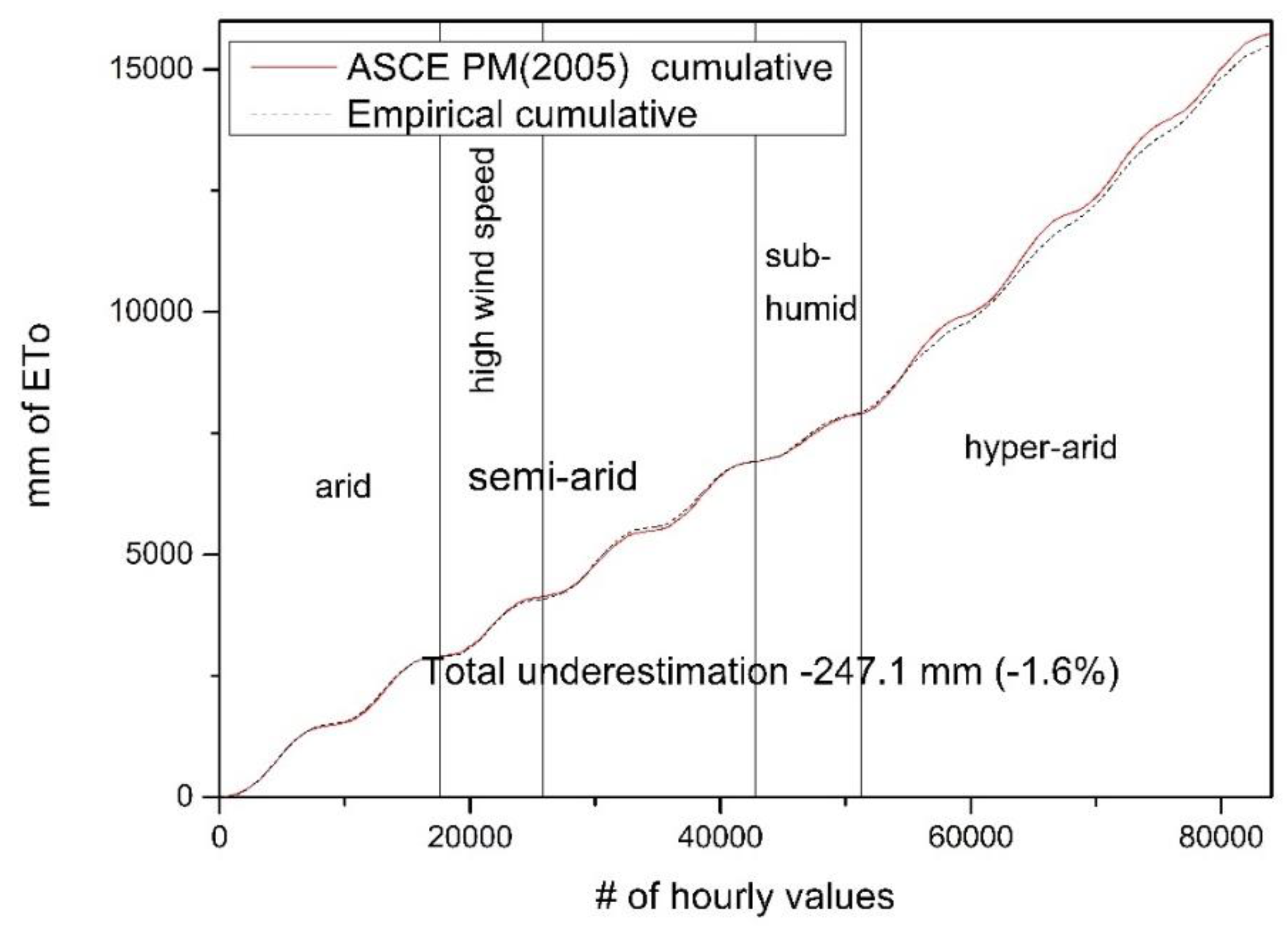
Figure 2.
Scatter plots of the estimations of the two methods (X axis for ASCEA PM (2005) and Y axis for the estimations of the empirical method) for the four hyper arid stations chosen from the CIMIS network (a Indio 2, b Cadiz, c Seeley, d Oasis). Aridity Index values ranged from 0.00 (Indio 2 station) to 0.04 (Seeley station).
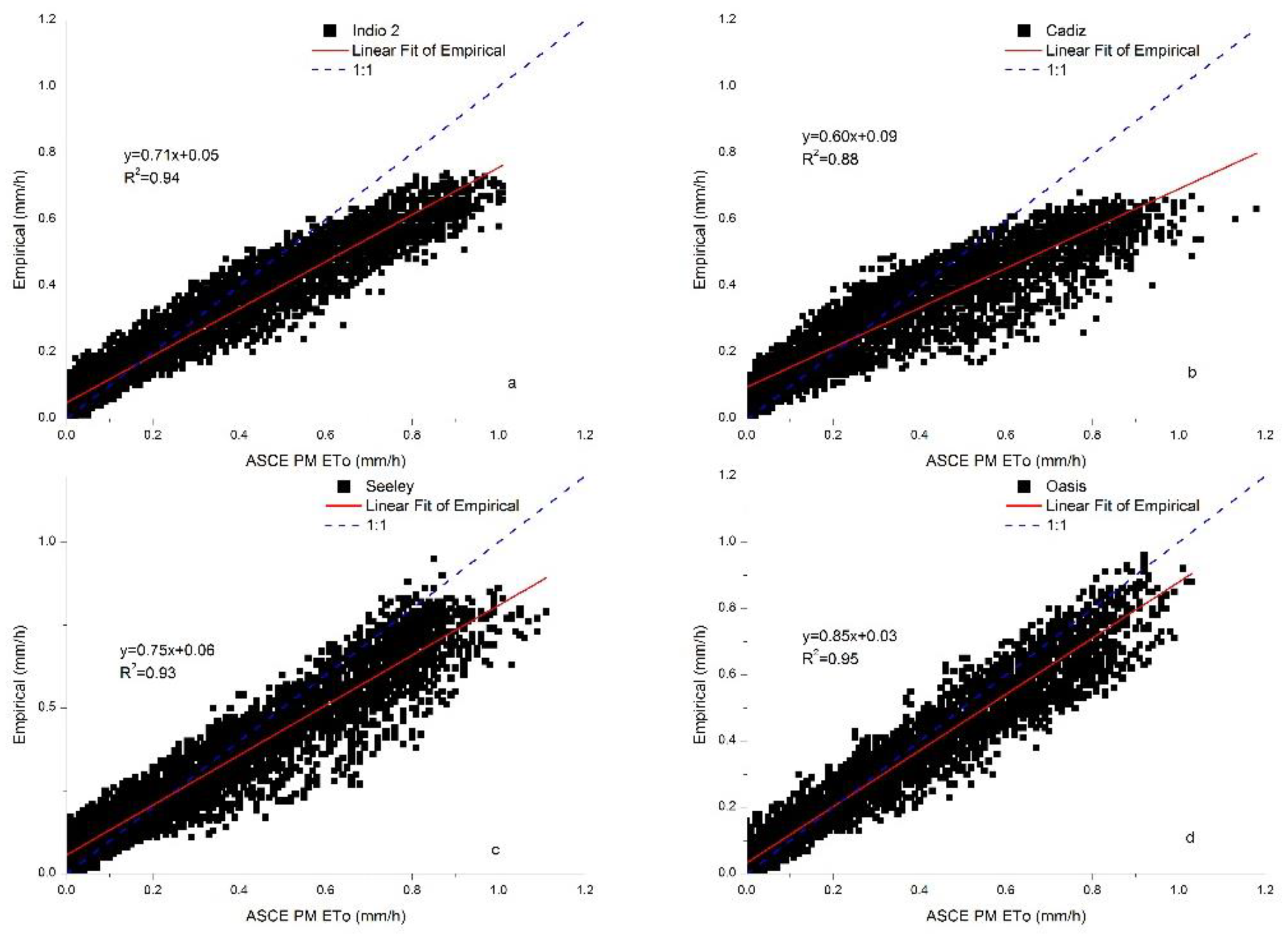
Figure 4.
Scatter plots between the two methods (X axis: ASCE PM (2005), Y axis: Empirical method), for the six CIMS stations with arid (Five Points station, Fresno station), semi arid (Colusa station, Durham station, Twitchel island station) and sub humid (Santa Rosa station) climatic conditions totaling 51249 hourly record for all the six stations.
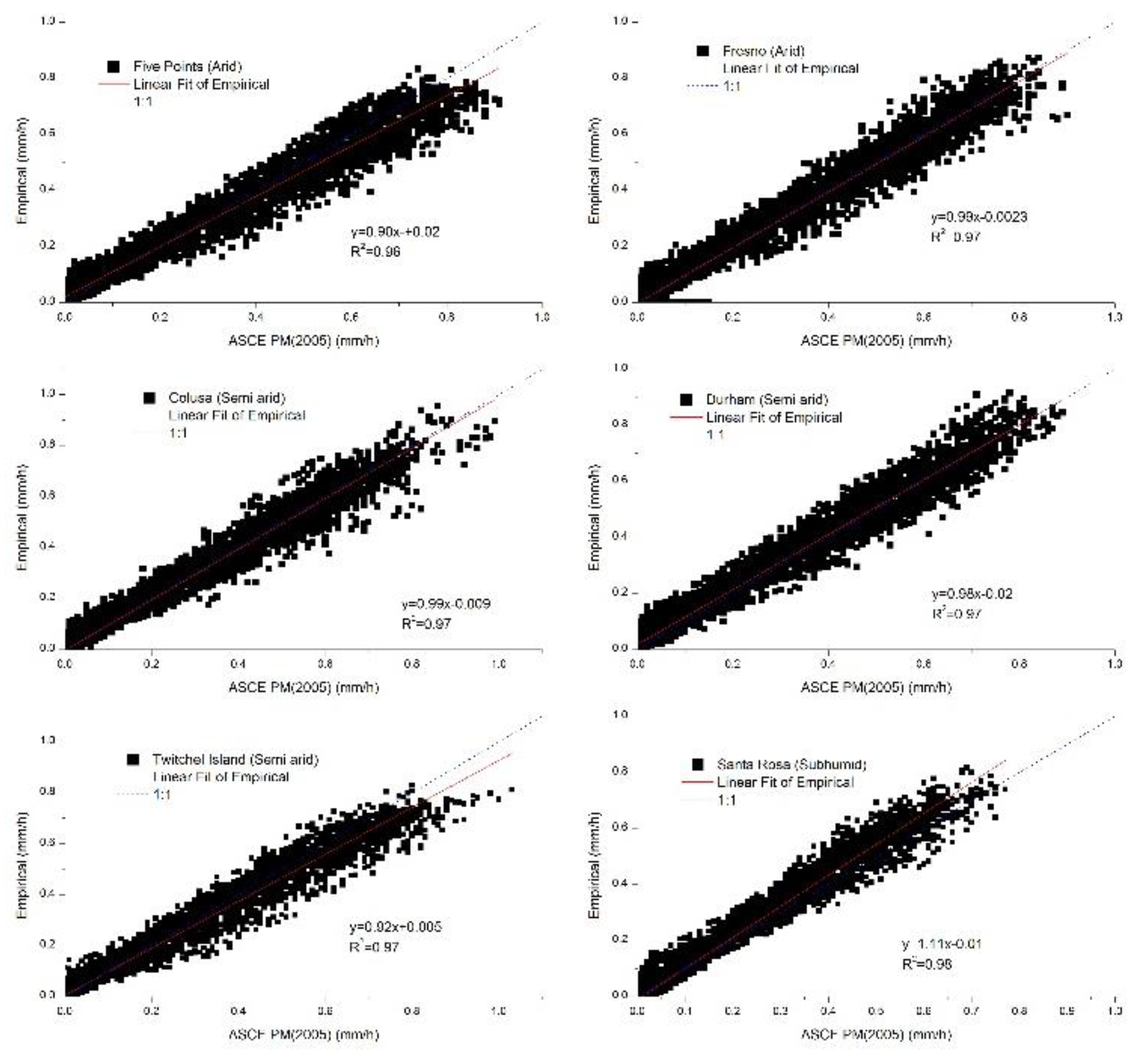
Figure 5.
Plots of the hourly values of the values of the empirical method (blue line) and of the values of the ASCE PM (2005) method (black line) for stations with arid and hyper arid climatic conditions, for DOY 170-175 (19 -24 of June) for the respective year of each station.
Figure 5.
Plots of the hourly values of the values of the empirical method (blue line) and of the values of the ASCE PM (2005) method (black line) for stations with arid and hyper arid climatic conditions, for DOY 170-175 (19 -24 of June) for the respective year of each station.
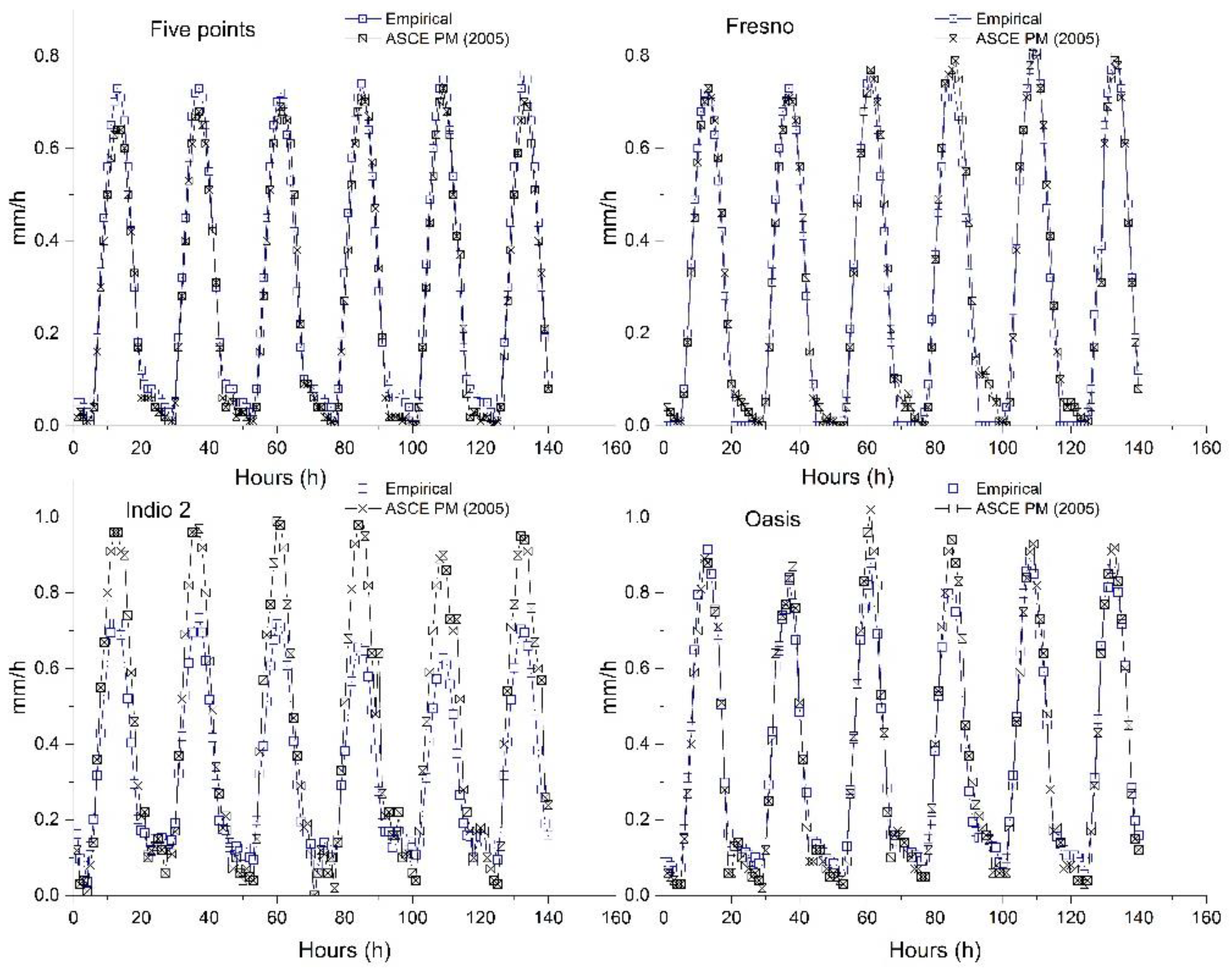

Table 1.
Meteorological station (CIMIS) studied for this paper. 83807 records (hourly) from 10 meteorological stations were analyzed. The selection was based on the criteria described in the right end column of the table. The AI (yearly Precipitation dived by Reference Evapotranspiration) is given for all the stations. Stations 221 (Cadiz Valley), 68 (Seeley) and 136( Oasis) are under hyper arid climatic regimes.
| Stn Id | name | long. | lat | elev (m) | Year | # of records | AI (P/ETo) | Remarks |
|---|---|---|---|---|---|---|---|---|
| 200 | Indio 2 | 33.75 | -116.25 | 12 | 2008 | 8235 | 0.00 | Hyper arid |
| 190 | Five Points | 36.38 | -120.23 | 82 | 2005 | 8759 | 0.10 | arid |
| 80 | Fresno | 36.82 | -119.74 | 103 | 2000 | 8783 | 0.20 | arid |
| 32 | Colusa | 39.23 | -122.02 | 16 | 2000 | 8254 | 0.34 | semi arid |
| 12 | Durham | 39.61 | -121.82 | 130 | 2001 | 8664 | 0.45 | semi arid |
| 83 | Santa Rosa | 38.40 | -122.80 | 24 | 2011 | 8471 | 0.74 | sub humid |
| 221 | Cadiz Valley | 34.51 | -115.51 | 47 | 2011 | 8741 | 0.03 | high VPD |
| 140 | Twitchel island | 38.12 | -121.66 | -1 | 2000 | 8318 | 0.23 | High wind speed |
| 68 | Seeley | 32.76 | -115.73 | 12 | 2011 | 7679 | 0.04 | High ETo |
| 136 | Oasis | 33.52 | -116.16 | 4 | 2005 | 7903 | 0.03 | Max Temp |
Table 2.
Annual totals for the empirical method and ASCE PM (2005) were calculated, their difference, their difference as a percentage (%) of the ASCE PM (2005) annual total, and the statistical indices of the empirical method against the ASCE PM (2005) for all the 10 station of the CIMIS network (83807 hourly records). The statistics in the last row were calculated using all (83807) the data.
| Station | Emp (mm yr-1) | PM (mm yr-1) | Emp-PM | (Emp-PM)% | R2 | RMSE | slope | ΙοA |
|---|---|---|---|---|---|---|---|---|
| Indio 2 | 1825.8 | 2019.4 | -193.7 | -9.6% | 0.94 | 0.095 | 0.71 | 0.957 |
| Five Points | 1502.2 | 1479.6 | 22.6 | 1.5% | 0.96 | 0.046 | 0.90 | 0.989 |
| Fresno | 1389.4 | 1422.0 | -32.6 | -2.3% | 0.97 | 0.038 | 0.99 | 0.993 |
| Colusa | 1189.2 | 1233.7 | -44.5 | -3.6% | 0.97 | 0.037 | 0.99 | 0.993 |
| Durham | 1477.6 | 1350.9 | 126.8 | 9.4% | 0.97 | 0.040 | 0.98 | 0.991 |
| Santa Rosa | 999.3 | 980.1 | 19.3 | 2.0% | 0.98 | 0.033 | 1.11 | 0.992 |
| Cadiz Valley | 2108.1 | 2141.9 | -33.8 | -1.6% | 0.88 | 0.115 | 0.60 | 0.919 |
| Twitchel island | 1368.1 | 1434.1 | -66.0 | -4.6% | 0.97 | 0.041 | 0.92 | 0.991 |
| Seeley | 1877.6 | 1916.4 | -38.9 | -2.0% | 0.93 | 0.088 | 0.75 | 0.968 |
| Oasis | 1749.3 | 1755.7 | -6.4 | -0.4% | 0.95 | 0.062 | 0.85 | 0.983 |
| Average | 1548.7 | 1573.4 | ||||||
| Total (83807 records) | 15486.6 | 15733.7 | -247.1 | -1.6% | 0.95 | 0.060 | 0.88 | 0.978 |
Table 3.
Values of slope, intercept, R2, RMSE, between the VPD and 1/ln(RH) values, for the four hyper arid stations (Indio 2, Cadiz, Seeley, Oasis, first four rows of the table) and for the all of the hourly values of the four stations (last row). The total of the hourly values (column 1) was divided into Warm period (column 2) and Cold period (column 3) for all the four stations and for all the hourly values of the four stations. The calculations were repeated for values grouped on a daily basis (Column 4).
| All hourly values (1) | Warm period (2) | Cold period (3) | Daily values (4) | |||||||||
|---|---|---|---|---|---|---|---|---|---|---|---|---|
| Slope | Intercept | R2 | Slope | Intercept | R2 | Slope | Intercept | R2 | Slope | Intercept | R2 | |
| Indio 2 | 0.0239 | 0.2343 | 0.61 | 0.0235 | 0.2284 | 0.61 | 0.0327 | 0.2304 | 0.66 | 0.0365 | 0.2192 | 0.93 |
| Cadiz | 0.0256 | 0.2671 | 0.51 | 0.0249 | 0.2654 | 0.46 | 0.0359 | 0.2569 | 0.49 | 0.0471 | 0.2388 | 0.88 |
| Seeley | 0.0175 | 0.2425 | 0.45 | 0.0181 | 0.2337 | 0.56 | 0.0266 | 0.2390 | 0.46 | 0.0290 | 0.2296 | 0.88 |
| Oasis | 0.0248 | 0.2263 | 0.67 | 0.0236 | 0.2263 | 0.61 | 0.0338 | 0.2205 | 0.80 | 0.0325 | 0.2162 | 0.96 |
| All stations | 0.0249 | 0.2395 | 0.52 | 0.0253 | 0.2314 | 0.54 | 0.0339 | 0.2357 | 0.54 | 0.0366 | 0.2262 | 0.91 |
Table 4.
Wind speed and VPD values with RMSEs lower than the limits set in this study (0.073 mm/h 0.113 mm/h) for hyper arid, arid, semiarid and subhumid climatic conditions with the percentages on the total number of values. The first column gives the percentage on all the records (83807) used for this study.
| u2 | |||||
| RMSE (mm h-1) | All hourly records | hyper-arid | arid | semi arid | sub humid |
| 0.073 | (5 m s-1) 94% | (2.2 m s-1) 60% | (6 m s-1) 99% | 100% | 100% |
| 0.13 | (8 m s-1) 99% | (5.3 m s-1) 94% | 100% | 100% | 100% |
| VPD | |||||
| RMSE (mm h-1) | All hourly records | hyper-arid | arid | semi arid | sub humid |
| 0.073 | (2.5 kPa) 87% | (2.1 kPa) 59% | 4.5 (kPa) 98% | (3 kPa) 97% | 100% |
| 0.13 | (7.5 kPa) 100% | (4.1 kPa) 86% | 100% | 100% | 100% |
Disclaimer/Publisher’s Note: The statements, opinions and data contained in all publications are solely those of the individual author(s) and contributor(s) and not of MDPI and/or the editor(s). MDPI and/or the editor(s) disclaim responsibility for any injury to people or property resulting from any ideas, methods, instructions or products referred to in the content. |
© 2025 by the authors. Licensee MDPI, Basel, Switzerland. This article is an open access article distributed under the terms and conditions of the Creative Commons Attribution (CC BY) license (http://creativecommons.org/licenses/by/4.0/).
Copyright: This open access article is published under a Creative Commons CC BY 4.0 license, which permit the free download, distribution, and reuse, provided that the author and preprint are cited in any reuse.


