
Submitted:
16 April 2025
Posted:
17 April 2025
You are already at the latest version
Abstract
The research context of this study focuses on optimizing the use of C60 steel in industrial applications where durability and fatigue resistance are critical. C60 steel is known for its combination of strength and hardness, but it is essential to evaluate how thermal and thermo-chemical treatments affect its performance under fatigue condi-tions.
The objectives of the study include: Investigating the crack formation process and the early stages of fatigue in C60 steel, comparing the effects of thermal treatments (hardening and tempering) with those of thermo-chemical treatments (oxidation) on the steel's micro-structure, evaluating the performance of C60 steel under fatigue conditions based on the applied treatments, providing insights that can help optimize the use of this steel in in-dustries requiring high resistance and durability.
The methodology of the study included: fatigue tests performed on a four-point bending machine to determine the exact time of microcracking. The C60 steel samples were pro-cessed according to SR ISO 1099:2017 "Fatigue testing. Axial load method". To ensure consistency and comparability of results, the samples were made from the same material charge and machined under the same conditions. A total of 26 specimens were used, 13 for each type of treatment: thermal treatment by hardening and tempering and thermo-chemical treatment by oxidation.
Due to the different mechanical properties obtained from the thermal and thermo-chemical treatment processes, the sets of specimens were tested at varying forces. In these tests, frequency changes were monitored to evaluate the behaviour of the materials under repeated stresses.
Finally, the frequency changes were correlated with the number of cycles to identify when microcracks appeared and their evolution.
The main results from this study show: significant differences between the lifetimes of thermally and thermochemically treated samples and the time of microcracks appear-ance in the material.
Keywords:
fatigue resistance
; computed tomography
; microstructure
; macro-structural analysis
; thermal and thermochemical treatments
1. Introduction
Steels are thermally and/or thermochemically treated to improve their mechanical properties. The structural changes induced by these treatments increase the resistance of steels to cyclic stresses. Fatigue testing allows the evaluation of the ability of materials to withstand repeated stresses and to identify when microcracks may appear. Microcrack initiation generally occurs at points where one or more stress concentrators, such as inclusions, blowholes and dents due to improper machining, voids and lattice defects, are present. Some authors, such as Cheng [1], have proposed semi-analytical methods for the prediction of the number of cycles required for crack initiation, which have been confirmed by experimental results.
To predict the fatigue resistance of different steels, Agrawal [2] used neural networks, decision trees and multivariate polynomials as data processing tools. The result was a more accurate assessment than classical prediction methods.
A state-of-the-art review of metal fatigue is carried out in [3], with particular emphasis on the latest developments in fatigue life prediction methods. All factors affecting the fatigue life of metallic structures are grouped into four categories: material, structure, loading and environment.
Crack initiation is considered the stage at which a defect-free structure subjected to varying loads develops microcracks (nanocracks). This microscopic cracking process can be defined as crack initiation. In fracture mechanics, a fissure is a crack or discontinuity in a solid material, which can grow and propagate under varying loads, leading to material failure. Thus, crack initiation involves the initial appearance of microcracks under the influence of loads, which can subsequently grow and propagate, leading to more pronounced cracking and ultimately material failure. [4] Over the years, catastrophic fatigue-related accidents have been recorded, the costliest of which are aviation accidents [5]. For these reasons, the study of the fatigue behaviour of steels and the identification of nano-microcracks occurring in the material is a research priority. Given the serious consequences of the failures caused by crack propagation, researchers are compelled to seek methods to identify crack damage. Academia and industry have achieved damage identification with a lot of studies using structural vibration response [6,7,8].
In the paper [9] based on fracture mechanics models, the proposed model is capable of automatically identifying the main stages (i.e., initial crack, type I crack, type II crack, and break) in the formation of microcracks. Simultaneously, the proposed model bridges the gap between the AI-based image analysis and the physical crack propagation models, enabling the extraction of key information such as microcrack length and width, and further supporting the analysis of fatigue crack growth rates associated with various microcrack stages. The model could discover that in the initiation stage, the crack of TC4 titanium alloy grows at a fairly slow rate (∼3.6 μm/cycle) and occupies most of the crack life cycle. After the initiation stage, the crack first propagates as the type I cracks with a significantly faster crack growth rate (∼50 μm/cycle).Then, the type II crack occurs with a substantially reduced growth rate (∼25 μm/cycle). In the final stage, as the microcrack reaches a critical size, the growth rate increases sharply, leading to break.
In paper [10] presents a multi-task deep learning framework called MT-CrackNet designed for the automated detection and measurement of in-situ fatigue micro-cracks, enabling real-time tracking and quantification of micro-cracks during in-situ fatigue tests.
According to Reifsneider [11], who has studied the long-term behaviour of composite materials and structures subjected to time-varying mechanical, thermal and chemical influences, material fatigue is a permanent, localized, progressive structural change that occurs in materials subjected to alternating stresses and results in cracking or failure of the material after a sufficient number of cycles.
Much extensive research is looking at how thermal or thermochemical treatment can improve fatigue resistance. The correct choice of thermal treatment brings the microstructure and mechanical properties of steel to optimum values and increases fatigue resistance. In this paper [12], fatigue crack initiation was evaluated on cylindrical samples which were subjected to fatigue tests with certain amplitudes. A fatigue crack initiation study was carried out by stopping cycles at a defined number and studying the surfaces using scanning electron microscopy. The researchers found that cyclic deformation was localized to the first interval. Other authors tried to study the increase in fatigue resistance by using AHSS (advanced high-strength steels) subjected to different thermal treatments. The increased fatigue resistance was studied by using advanced high-strength steels with different thermal treatments. Kwon et al. studied the mechanical and fatigue properties of a conventional 0.25% C, 0.42% Si, 0.82 Mn and a modified 0.33% C, 0.51% Si and 1.51 Mn steel thermally treated by hardening depending on the variation of the tempering temperature. The two types of steels were subjected to hardening at 950 °C and tempering between 100 and 340 °C. The machined specimens of conventional steel were tempered at 340°C for comparison and the modified steel specimens were tempered at 100, 200, 250, 300, 340 and 400°C for tension specimens and at 100, 250 and 340°C for fatigue specimens. From the experiments, the authors found that the specimen that was tempered at 100°C had the lowest fatigue resistance due to the fully martensitic microstructure, which behaves as a brittle material and the steel hardened at 250°C showed the best fatigue results due to the presence of carbide particles that acted as a retarder of dislocation build-up at the lateral boundaries, having a beneficial effect on fatigue properties. [13]
The fatigue resistance of thermally treated 60Si2CrVAT spring steel was studied in [14], in which the authors analysed the microstructure and fatigue failure surface area using scanning and electron microscopy methods.
It is well known that thermochemical treatments produce high-hardness layers on the surface of steel that are stressed in compression. This explains why increasing the hardness and surface resistance by nitriding or nitrocarburizing increases the fatigue resistance of the parts. Sometimes, changes in the chemical constituents in the microstructure of the material at the surface layer can adversely affect fatigue resistance.
The paper [15] demonstrates that Cracks originate in the surface oxide layers, which are inherently brittle and subjected to the highest tensile stress, leading to early fatigue crack initiation, while oxygen ingress through it causes rapid crack propagation.
The article [16] details both the positive and negative effects of the thermochemical pre-oxidation treatment.
The dependence of material fatigue on the material structure (phase transformations, grain boundary slippage, pore nucleation, microcrack formation, structural defects, inhomogeneities, non-metallic inclusions and chemical composition) is extremely important because traditional theories of fracture mechanics are based on the concentration factors produced by structural defects [17]. Thus, in [18], the authors detail the crack size and the degree of fatigue damage by making observations on crack initiation and growth. Crack propagation is controlled by the stress level, the maximum stress introduced into the material and occurs through a process of repeated deformation and failure near the crack tip. With increasing crack length, the deterioration process is accelerated. There are situations where, due to the low-stress level, the crack propagation process ceases. The fatigue life of a structure is provided by the number of stress cycles after which failure occurs. The current method of estimating the fatigue life of structures is to calculate the equivalent stress amplitude from measured stress data. To assess fatigue damage, a new method has been established to calculate the equivalent stress amplitude [19].
Investigations into crack depth when there is a frequency decrease on unnotched and notched samples in [20] and [21] have shown that stress-controlled tests on notched flat specimens (Kt=2.5 and 4.6) conclude at a frequency drop of 0.3 Hz. In this case, there is a crack on both sides of the specimens, each with a depth of 3 to 6 mm. In most cases, the specimen breaks beforehand. In the case of unnotched flat specimens, the frequency decreases so rapidly after the appearance of a crack that there are only a few hundred cycles between the determined number of interruption vibration cycles and the actual number of crack initiation cycles. According to [22], the technical crack is defined for strain-controlled tests at a load drop of 10% on the established hysteresis loop. In specimens or components, fatigue cracks usually originate from the surface. There are various reasons for this. It has been proven that surface roughness can have a decisive influence on vibration resistance behavior [23] and [24].
2. Materials and Methods
The work to be completed and an experimentation plan were established in a logical succession of steps, as presented in Table 1. The investigations were carried out in several enterprises and research institutions. Following these experiments, the dependence between the heat treatments applied and the fatigue test parameters was highlighted.
2.1. Sample Processing
The C60 material was purchased in hardened and tempered condition, with a ultimate tensile strength (UTS) of 1333 MPa, in the form of a platband with the dimensions of 110x14x3 mm (LxWxH) from Zelos Zerspanung in Bessenbach, Germany. The samples were processed according to SR ISO 1099:2017 “Fatigue testing. Axial load method” [25] (Figure 1).
2.2. Chemical Composition
The determination of the chemical composition was carried out using high-resolution spark spectrometry, utilizing the SPECTROMAXx spectrometer from the Liebherr
Deggendorf Laboratory. We conducted 9 measurements to obtain precise and relevant values, essential for the detailed characterization of the material.
The chemical composition of the alloy is presented in Table 2.
2.3. Identification of Specimens
To ensure optimal traceability, the samples were laser-marked using the WeLase- Laser- Workstation equipment from the Testing Department of Fa. Liebherr Deggendorf, with each sample being identified by a unique number.
2.4. Fatigue Testing
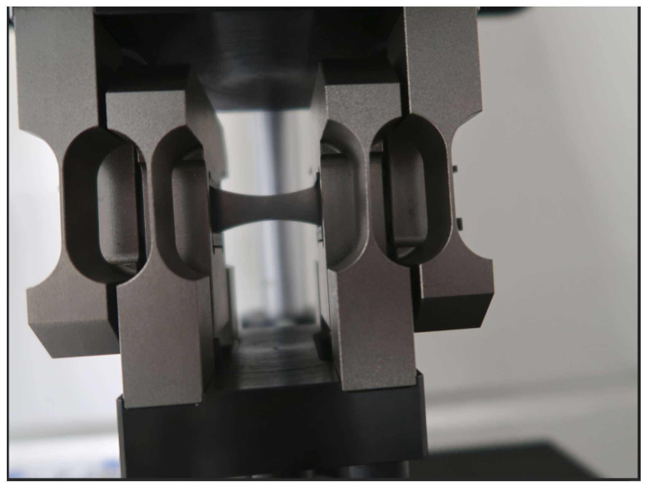
For fatigue testing 26 specimens were purchased for the study, of which 13 were tested as delivered and the remaining 13 were tested after thermochemical oxidation treatment. The samples were then subjected to fatigue tests at Fa. Liebherr Deggendorf, using a 100 Nm (20 kN) MIKROTRON four-point bending machine (4-Punkt-Biegvorrichtung), specifically designed for fatigue testing (Figure 2). The machine is capable of fatigue testing at a frequency up to 140 Hz. In these tests, the stress frequencies for all tests were 127±10 Hz. The evaluation of tests in the present article conducted under voltage control is carried out exclusively within the domain of temporary fatigue resistance. In this case, the material has the ability to withstand repeated cyclic loading for a certain number of cycles before the appearance of a crack. This method differs from unlimited fatigue resistance, where the material can endure a very high number of cycles without suffering significant deterioration. For all tests conducted, a reduction in the testing frequency by 0.1 Hz has been established as the crack initiation criterion, while a reduction of 1.2 Hz has been set as the failure criterion, defining the critical threshold for assessing the system’s behavior under stress conditions. The frequency decrease of 0.1 Hz, based on empirical experience, ensures a precise and reproducible methodology, facilitating a detailed analysis of variations in test parameters.
Figure 3 show the following:
- In the four-point bending test, the sample is supported in pairs of two points. Counter nuts are used to eliminate gaps since the tests were performed in an alternating cycle.
- The gripping areas in the testing machine wedge grips are machined by milling to align the wedge grip and test sample with the direction of the loading force.
- Tightening of the testing machine wedge grip is carried out hydraulically, thus ensuring firm clamping and preventing slippage or dropping of the sample from the wedge grip when the force is reversed. Under these conditions, it can be stated that the specimen axis is correctly aligned with the direction of the loading force and that all gripping elements are properly tightened, eliminating gaps between the specimen’s clamping components.
Figure 3.
Sample wedge grip.
3. Experiment
3.1. Evolution of the Microstructure as Delivered
A cross-sectional section was cut from the delivery state sample (Figure 4) using a QATM Brillant 220 machine equipped with a SiC cutting wheel at a low speed (0.05 mm/s) to avoid introducing stresses into the sample. The cut sample was then placed in the OPAL x-Press hot mounting machine from QATM. The samples underwent primary grinding to achieve a smooth surface, starting with coarse grit abrasive papers (P180) and progressing to fine grit (P1800). Finally, the samples were polished to obtain a very smooth and reflective surface using Mono diamond suspension.
The microstructural analysis of the sample in the delivery state was performed by light microscopy, using the Axio Imager 2 microscope at x100-1000 magnification from Carl Zeiss Microskopy Deutschland.
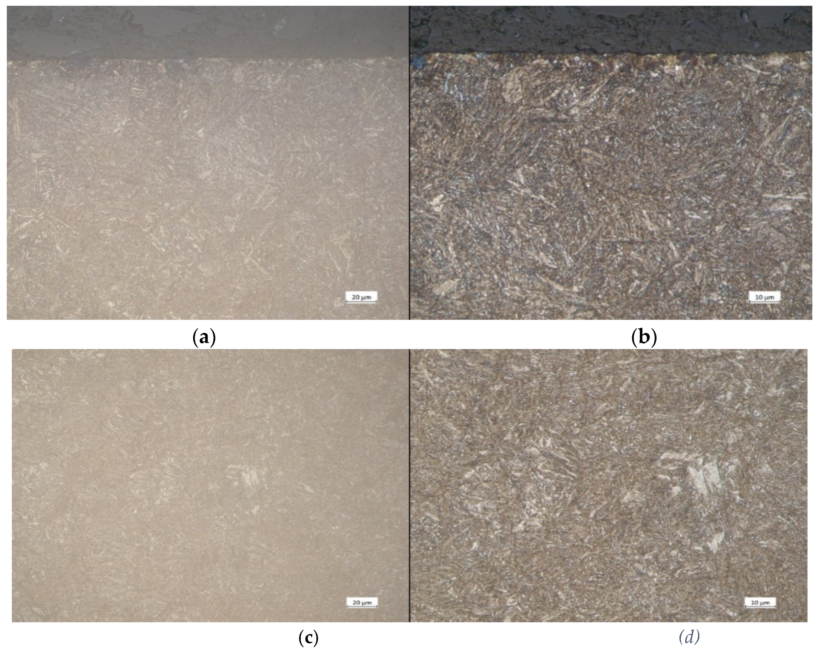
The process involved washing the sample with water, degreasing it with alcohol, drying and etching with a 3% Nital solution. Etching was stopped (when the surface became matte) by washing the sample under a water spray, spraying with ethanol and rapid drying with hot air. To verify that the thermal treatment applied was uniform over the entire section of the part, the sample was metallographically investigated both at the edge and the core. The samples thus prepared are shown in Figure 5.
From the metallographic analysis of the material as delivered, a sorbitic structure consisting of a ferritic matrix and uniformly distributed iron carbides (cementite) is observed. No variations in the microstructure of the material were observed either at the surface of the part or in its core. Detailed metallographic analyses, performed both at the edge and in the core of the sample, showed a structure characteristic of hardened and tempered steel. Therefore, it can be concluded that the hardness of the C60 steel purchased hardened and tempered is consistent with the metallographic structure.
Figure 5.
Microstructure of C60 steel as delivered – thermally treated by hardening and tempering a) microstructure at the edge of the part at a magnification of 500x - sorbite, b) microstructure at the edge of the part at a magnification of 1000x - sorbite, c) microstructure at the core of the part at a magnification of 500x and d) microstructure at the core of the part at a magnification of 1000x.
3.2. Hardness Measurements
The hardness of the piece was tested both on its surface using the Brinell method HBW 2.5/187.5 with the KB 250BVRZ device from Härterei Reese Brackenheim, and in its core using the Vickers method HV30 with the KB30S device. The obtained results were converted into MPa according to DIN EN ISO 18265, Table B2 units for more precise and comparable interpretation.
Table 3 shows that the sample has a surface hardness of 415 HBW, corresponding to a mechanical strength Rm of 1312 MPa and a core hardness of 424 HV 30, corresponding to a mechanical strength Rm of 1322 MPa, converted according to DIN EN ISO 18265, Table B2 (average value of three measurements).
3.3. Thermochemical Oxidation Treatment
In this process, the top layer of the material is treated in an oxidizing atmosphere to create a protective oxide layer. Nitrogen (N₂) was used as the carrier gas to control the atmosphere. During oxidation, water was introduced into the furnace to promote the formation of the oxide layer. After oxidation, the samples were slowly cooled to minimize stresses in the oxide layer.
After thorough cleaning, the metal parts were placed in the furnace and arranged so that they did not overlap. The thermal oxidation of the steel was carried out at a constant temperature of 500°C for 2,5 hours in Fa. Härterei Reese Brackenheim (Figure 6). The parameters of the process are presented in Table 4 und below.
This arrangement allowed uniform exposure of the parts to the oxidizing atmosphere, which resulted in the formation of a protective oxide layer.
After thermochemical treatment, the samples exhibit a black tint over the entire surface, highlighting the uniformity and efficiency of the oxidation process (see Figure 7 and Figure 8)
The microstructure examination was performed using light microscopy with the Axio Imager 2 microscope from Carl Zeiss Microscopy Deutschland, at a magnification of x1000.
To protect the oxide layer and to avoid its exfoliation during the preparation of the metallographic polished section, the samples were wrapped in aluminium foil.
Depth profiles of an oxidized sample were examined at the TAZ laboratory. For the analysis of the sample, glow discharge spectrometry was used with the Spectruma GDA750: HP device, and X-ray fluorescence analysis was performed using the Spectro Ametek: Cube D device.
Figure 9a shows the microstructure of the sample thermochemically treated by oxidation, where the presence of an oxide layer of approximately 4 µm on the surface of the part can be observed. In Figure 9b, in the core of the piece, due to maintaining the temperature at 500°C for about 2.5 hours followed by slow cooling, an intermediate bainitic structure can be observed [a mechanical mixture of supersaturated ferrite with carbon and carbides that have not reached the stage of cementite].
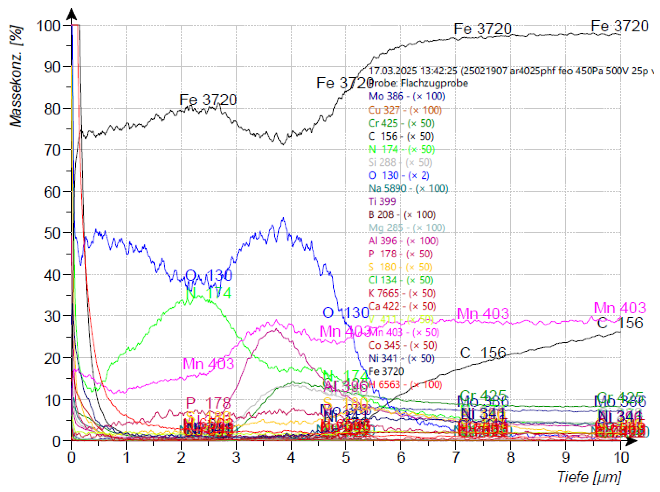
Figure 10 shows XRF measurements on the surface und GDOES-Measurements conducted Figure 11 and Figure 12.
In the layer, there are several zones with accumulations of oxygen-affine elements, such as aluminum, manganese, and silicon, or possibly, nitrogen-rich layers.
Figure 9.
a) Surface microstructure of C60 steel subjected to thermochemical oxidation treatment. b) Surface microstructure of C60 steel subjected to thermochemical oxidation treatment.
Figure 9.
a) Surface microstructure of C60 steel subjected to thermochemical oxidation treatment. b) Surface microstructure of C60 steel subjected to thermochemical oxidation treatment.
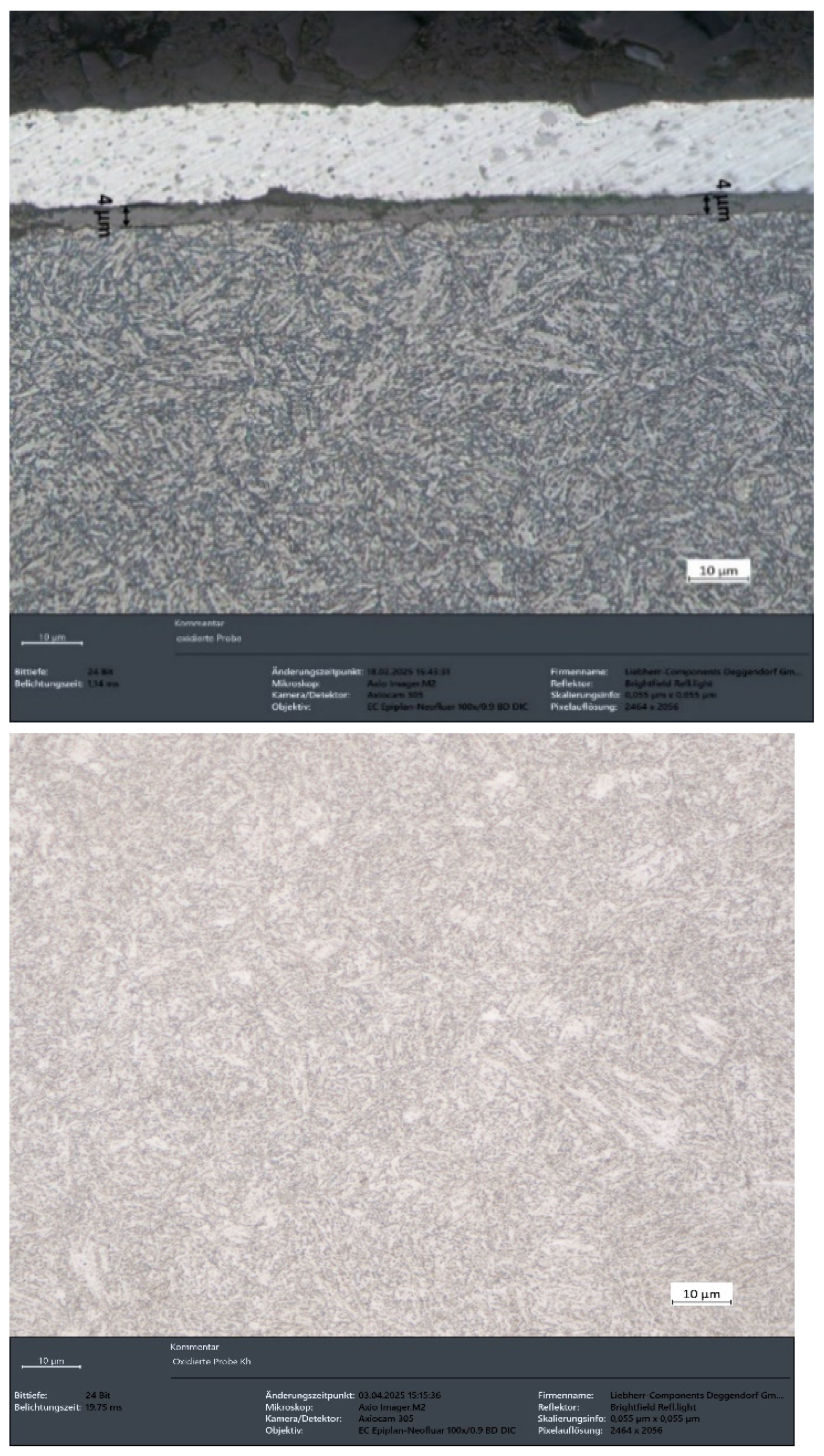
Figure 10.
Sampel XRF measurements on the surface, total spectrum up to 31 keV.
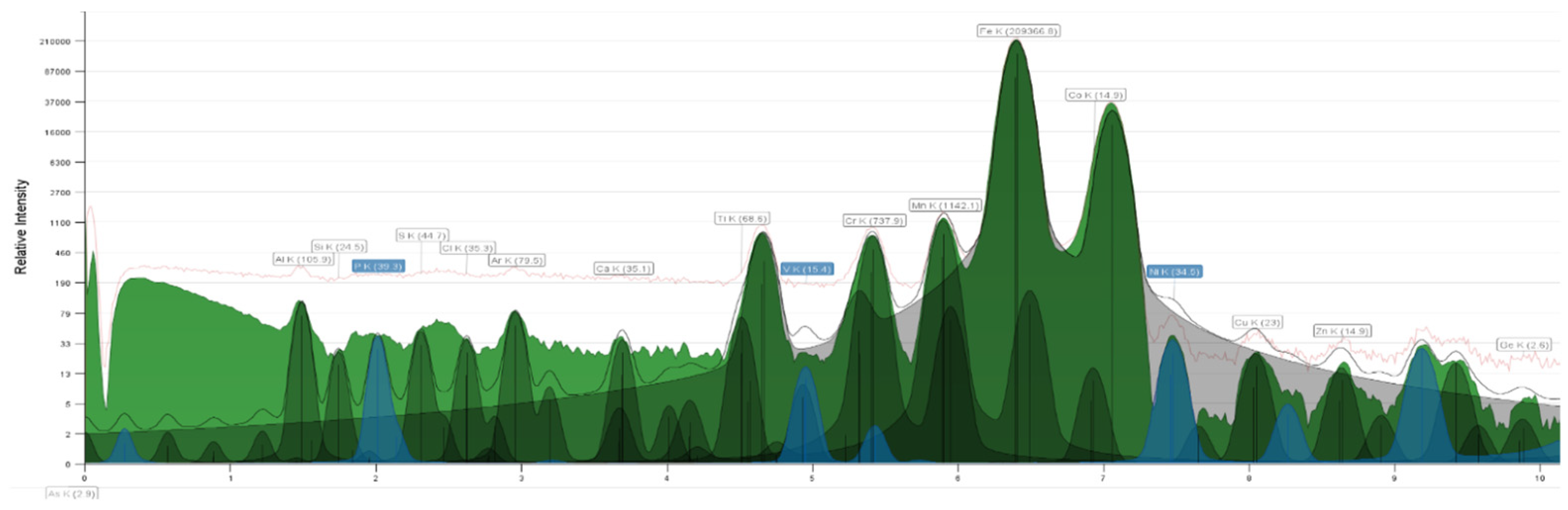
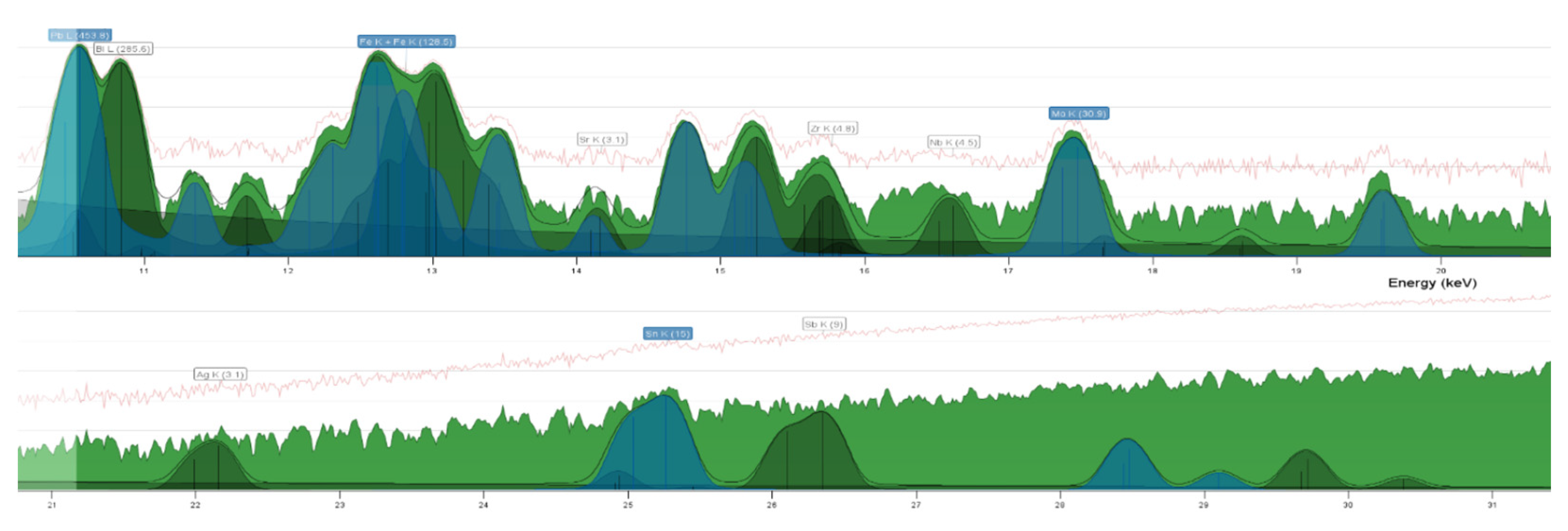
Figure 11.
GDOS-measurements 1.
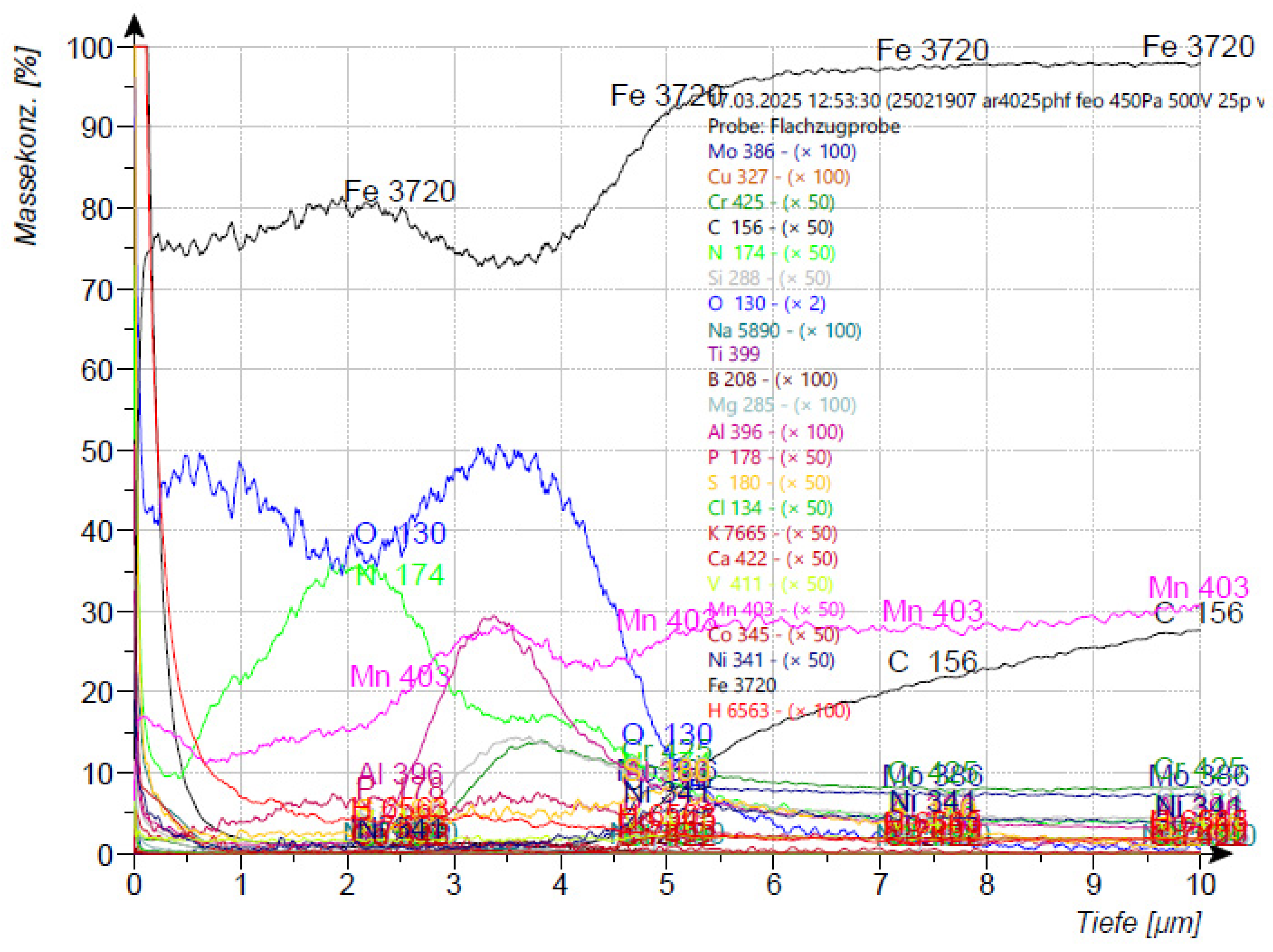
Figure 12.
GDOS-measurements 2.
3.4. Material Hardness Analysis After Thermochemical Oxidation Treatment
The hardness of the piece was tested both on its surface using the Brinell method HBW 2.5/187.5 with the KB 250BVRZ device from Härterei Reese Brackenheim, and in its core using the Vickers method HV30 with the KB30S device. The obtained results were converted into MPa converted according to DIN EN ISO 18265, Table B2 units for more precise and comparable interpretation. The surface of the piece was evaluated using a microhardness test HV 0.05 to determine if the thermochemical oxidation process influenced the hardness characteristics.
Table 5 shows that the sample has a surface hardness of 326 HBW, corresponding to a mechanical strength Rm of 1047 MPa and a core hardness of 294 HV 30, corresponding to a mechanical strength Rm of 920 MPa, converted according to DIN EN ISO 18265, Table B2 (average value of three measurements).The microhardness of the sample surface is 363 HV 0.05.
3.5. Surface Profilometry of Improved Specimens and Thermochemical Oxidation Treatment Specimen
The determination of roughness for the improved specimens and those treated through thermochemical oxidation was carried out by the 3D-Measurement Department of Liebherr Deggendorf, using the high-precision Zygo AMETEK device. This method enabled a detailed characterization of the surfaces, accurately highlighting the topographical changes induced by the applied treatments. The measurement results indicated a roughness of 0.974 µm for the improved specimens (Figure 13) and 0.861 µm for the oxidized sample (Figure 14). The surface roughness levels for both materials are comparable, with the improved material exhibiting lower roughness, while the thermochemically oxidized material shows slightly higher roughness. The increased roughness observed in the oxidized specimens is attributed to the formation of the oxide layer on the surface. Table 6 presents the results of roughness measurements for the improved specimens and the oxidized ones.

Table 6.
The results of roughness measurements for the improved specimens and the oxidized ones.
| Number of measurements | Rz [µm] | |
| Improved Sample |
Oxidized Sample |
|
| 1 | 0.843 | 0.626 |
| 2 | 0.868 | 0.821 |
| 3 | 0.982 | 1.229 |
| 4 | 0.734 | 0.807 |
| 5 | 0.545 | 0.824 |
| x̄=0.794 | x̄=0.861 | |
4. Result and Discussion
4.1. Failure testing for the Improved Material
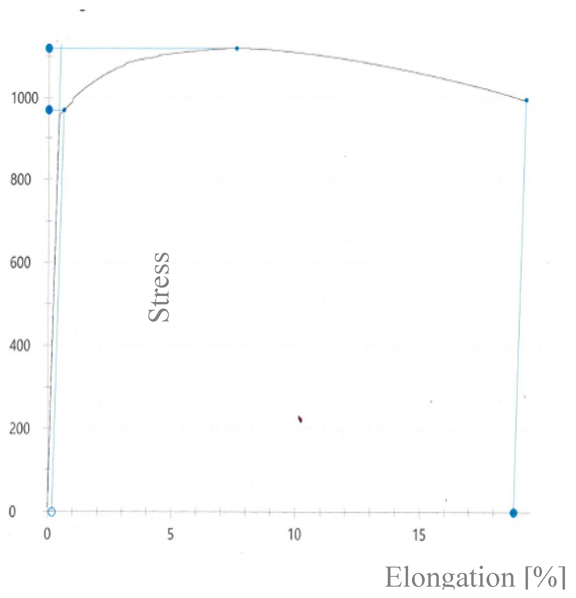
To define the characteristics of the improved material, the stress-strain curve was plotted Figure 15, on which the elongation (A), tensile strength (Rm) and yield strength (Rp 0.2) were determined using a Zwick Typ BT1-FR250SN.A4k, 25 kN, tensile-testing machine according to DIN EN ISO 6892-1. The characteristics of the material obtained as a result of the tensile strength are presented in Table 7.
Table 7.
The characteristics of the improved material.
| Probe | a0 [mm] |
b0 [mm] |
S0 [mm2] |
Le [mm] |
mE [GPa] |
Rp0,2 [MPa] |
Fm [kN] |
Rm [MPa] |
A10mm [%] |
| 01 | 3,04 | 8,02 | 24,38 | 10,01 | 206 | 1257 | 34,49 | 1415 | 6,0 |
4.2. Fatigue Test for the Improved Material
The tests were conducted and evaluated as follows: to identify the moment when microcracks initiate, the improved samples were subjected to cyclic loading, with continuous monitoring of frequency variation. A total of 13 samples were tested. Initially, fatigue tests were conducted on 3 reference samples, which failed after a specific number of cycles. Based on this data, an average number of cycles, presented in Table 8, was established as a baseline for testing the remaining 10 samples. These additional samples were evaluated under progressively increasing cycles at a consistent rate to observe the formation of the initial cracks.
To perform fatigue tests and evaluate the behaviour of the material under cyclic stress, it is essential to set up the testing machine correctly. This can be done by determining the maximum allowable stress introduced into the specimen or by accurately calculating the force applied to the samples. Based on the results of the tensile test, the tensile strength of the material was found to be approximately 1415 MPa. Under these conditions, the starting stress for testing the specimens was set at 920 MPa (equivalent to 0.65 of Rm), and the force was determined according to the bending moment [26] and the specifications of the tested material according to the relation
where:
where:
M=Rm·W [Nm]
M= 1331*32= 42592 Nm
F= 4.2 kN
- M is the bending moment,
- σadm - the maximum stress introduced into the specimen in the section to be fractured,
- b=8 mm - width of the calibrated portion,
- h=3 mm - thickness of the specimen,
- a=20 mm - the lever arm, which refers to the distance between the points of application of forces and the points of support,
- W - strength modulus of the cross-section (mm).
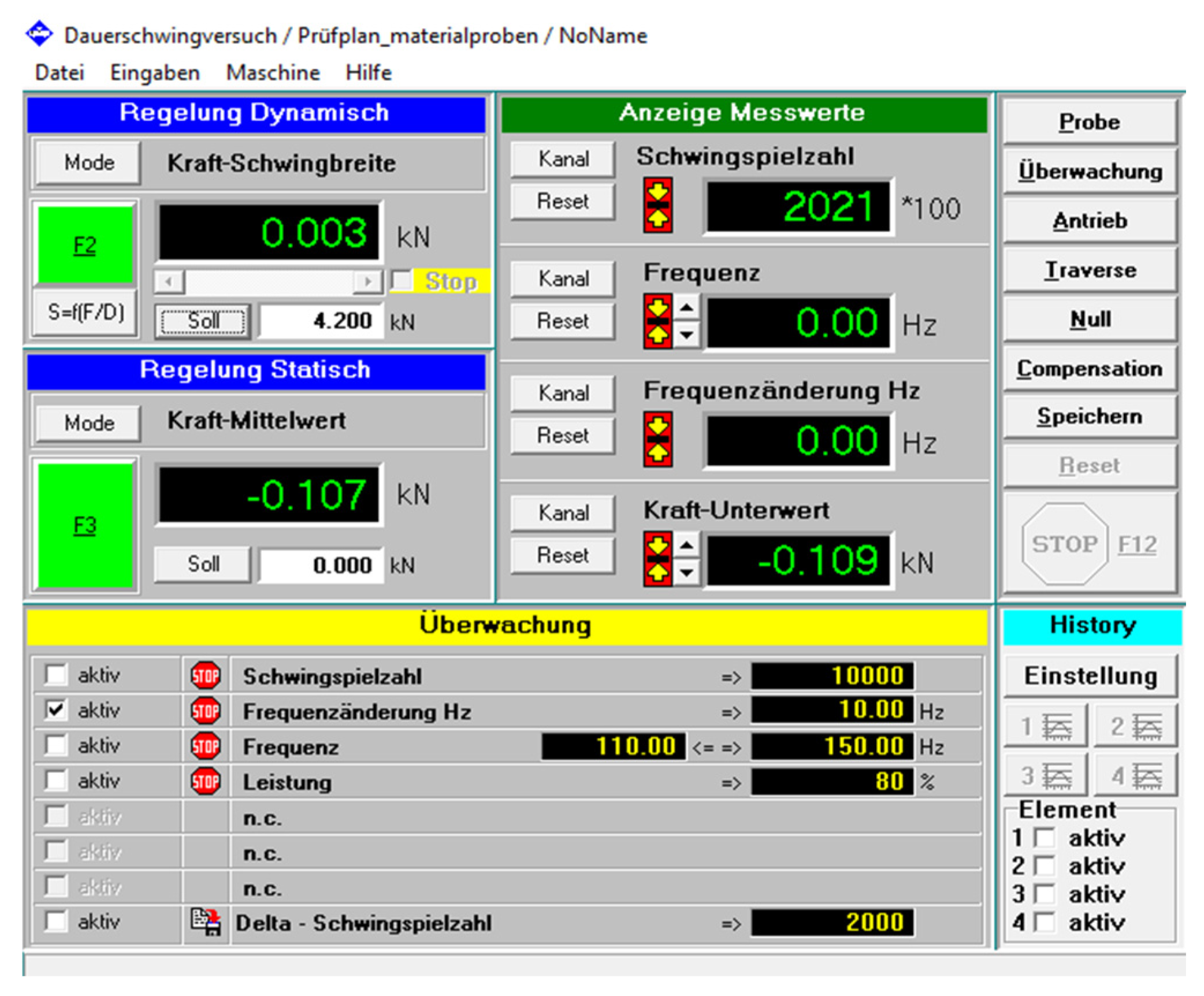
After adjusting the sample on the testing machine, the machine is set up by configuring the applied force, in this case, 4.2 kN. Figure 16
Also, the cycles at which the machine is desired to stop automatically are set and frequency changes are monitored to identify any microcracks or other structural changes in the material. The number of cycles and frequency are automatically recorded by the testing machine and tabulated. This functionality allows precise monitoring of the test parameters and ensures detailed documentation of the evolution of the samples during the experiment.
Figure 16.
Setting the test machine parameters.
According to the experiments, the moment of crack initiation is defined as the number of cycles for which a change in the stabilized maximum load is recorded.
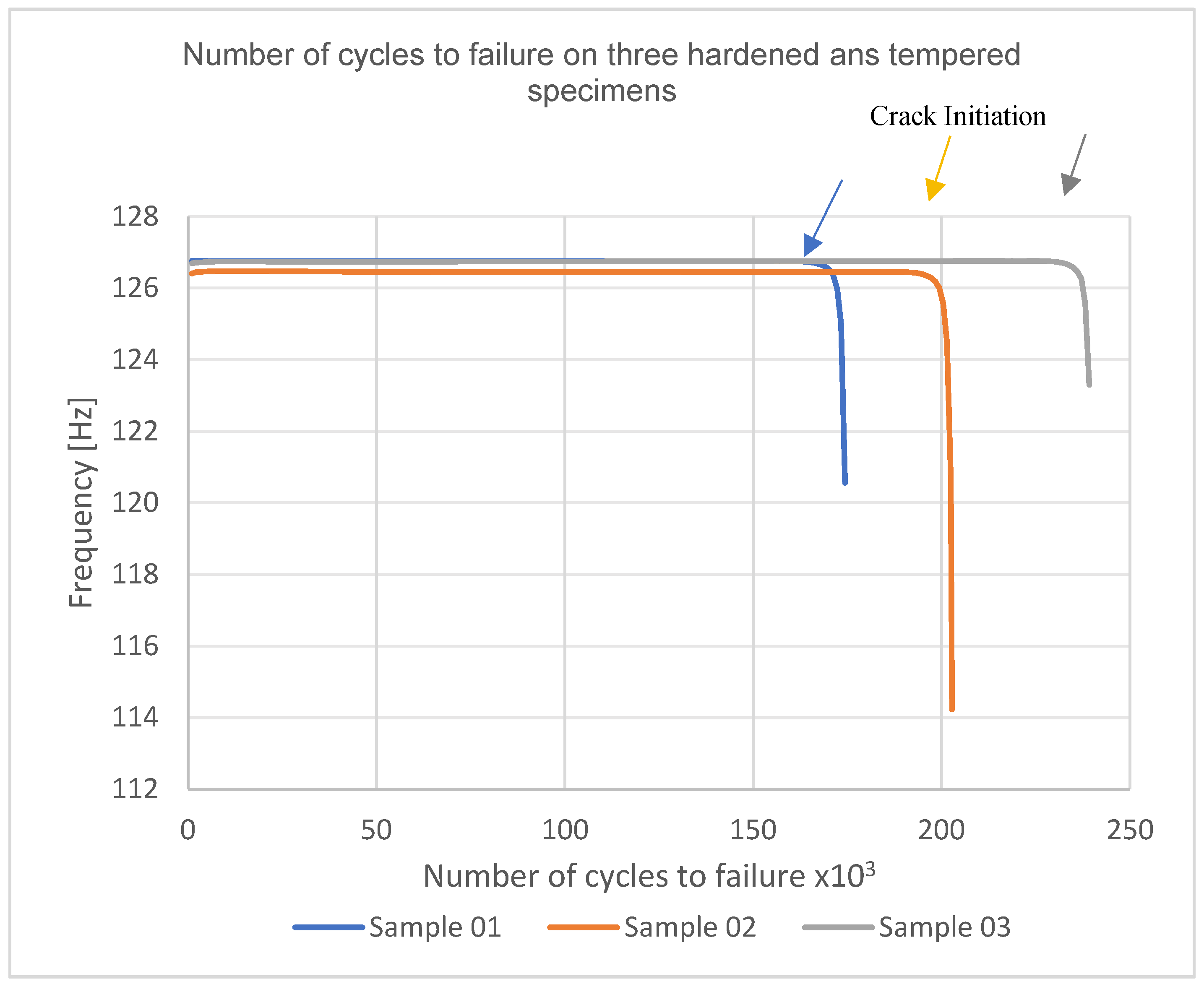
Table 9 shows the essential parameters, number of cycles to failure, and frequency changes for the three hardened and tempered reference samples. Figure 17 shows the failure diagram, highlighting the frequency variation and the maximum number of stress cycles, providing a schematic representation for a material that disintegrates.
This decrease in frequency indicates deterioration of the material subjected to stress cycles. The decrease in frequency signals that the material can no longer withstand the same repeated loads and is in an advanced state of fatigue, approaching the breaking point.
The table presents the evolution of frequency until failure, highlighting the results of tests conducted on samples 01, 02, and 03. These tests indicated a decrease in frequency, reaching a value of 7 Hz at the moment of failure. However, in all cases, the cracking of the samples occurs prior to this moment. The decrease in frequency can be correlated with the onset of the material’s cracking process. The table shows that the frequency changes for the three samples occurred alongside a decrease of 0.02 Hz, suggesting the beginning of structural deterioration.
Table 9.
Fatigue to failure test results for the hardened and tempered samples.
| No. of sample | No. total of cycles |
Initial frequency [Hz] |
Decrease in frequency [Hz] |
Final frequency [Hz] |
| 01 | 174600 | 126.760 | 126.736 | 120.558 |
| 02 | 202800 | 126.442 | 126.437 | 114.239 |
| 03 | 239700 | 126.709 | 126.674 | 123.297 |
| x̄=205700 | x̄=126,637 | x̄=126,615 | x̄=119,364 |
The diagram gives a clear insight into the behaviour of the material under cyclic stresses, allowing its durability under fatigue conditions to be evaluated. The diagram shows that the frequency remains constant up to a certain number of cycles at the beginning of the test, after which it starts to decrease. The decrease in frequency was identified at 163134 cycles for sample 01, 191177 cycles for sample 02 and 233013 cycles for sample 03
Figure 17.
Failure diagram for hardened and tempered samples.
In the paper” Influence of Edge Processing of Aluminum Sheets on the Residual Formability and Strength Properties under Quasi-static and Oscillating Loads - Research Center Chair of Forming Technology and Foundry, Technical University of Munich,” the evolution of the test frequency as a function of the number of cycles is schematically presented Figure 18 (Dittmann and Pätzold, 2018).
Figure 19 shows the hardened and tempered specimen tested to failure. It shows a visible crack without requiring CT inspection and the Figure 20 a illustrates the frontal view of the specimen following a fatigue load of 202800 cycles and Figure 20 b illustrates upper surface of the specimen. The fatigue crack was initiated in the upper region of the radius, the sample display individual notches along the cut edges at regular intervals, which are clearly noticeable, originating from a machining defect. Its progression is notable for its linear trajectory, with minimal branching or deviation observed. The crack length on the frontal surface of the specimen, measured from its edge, is documented as 5701 µm, corresponding to approximately one-third of the specimen’s total width.
Table 10 shows the number of cycles set for each of the 10 additional specimens and the frequency changes that occurred during the experiment, and Figure 21 shows a graph superimposing the 10 fatigue behaviour curves of the hardened and tempered specimens subjected to a predetermined number of stress cycles. This graph illustrates the variability in the fatigue behaviour of the specimens and provides essential information for understanding how the material responds to cyclic stresses. During testing, it was observed that the frequency remained constant for specimens 1 through 7, exhibiting uniform behaviour with minimal variation between them. However, a decrease in frequency with 0,14 Hz was observed for samples 8, 9 and 10, indicating a significant behaviour change.
Table 10.
Results obtained after fatigue testing with a predetermined number of cycles for the hardened and tempered samples.
Table 10.
Results obtained after fatigue testing with a predetermined number of cycles for the hardened and tempered samples.
| No. of sample | No. of cycles | Initial frequency [Hz] | Final frequency [Hz] |
|---|---|---|---|
| 1 | 20000 | 127.032 | 127.032 |
| 2 | 40000 | 127.034 | 127.034 |
| 3 | 60000 | 126.824 | 126.824 |
| 4 | 80000 | 126.908 | 126.908 |
| 5 | 100000 | 127.021 | 127.021 |
| 6 | 120000 | 126.900 | 126.900 |
| 7 | 140000 | 126.929 | 126.928 |
| 8 | 160000 | 126.930 | 126.826 |
| 9 | 180000 | 126.900 | 126.832 |
| 10 | 200000 | 127.200 | 126.924 |
4.3. Computed Tomography (CT) Analysis of the Improved Material After Fatigue Testing
To verify the hypothesis that the frequency drop indicates the appearance of microcracks in the material, we conducted a computed tomography (CT) inspection. This method allowed us to analyze the internal structure of the specimen in detail and confirm the presence of microcracks, thus validating our hypothesis.
Samples 8 in which a decrease in frequency was observed were tested with liquid penetrant and tomographic inspection. The liquid penetrant analysis showed the presence of a microcrack on one of the sides. On the other hand, computed tomography (CT) allowed detailed detection of the internal microcracks, providing additional information about their size and exact localization in the entire volume of the material, Figure 22.
From Figure 22, it can be observed that the sample initially presents a crack in the radius area, which subsequently extends to the frontal surface. This evolution of the crack highlights the critical points of the material and confirms the hypothesis that, with the decrease in frequency, a microcrack appears in the material.
4.4. Failure Testing for the Oxidized Material
To define the characteristics of the oxidized material, the stress-strain curve was plotted Figure 23, on which the elongation (A), tensile strength (Rm) and yield strength (Rp 0.2) were determined using a Zwick Typ UP-148525; 250KN, tensile-testing machine according to DIN EN ISO 6892-1. The characteristics of the material obtained as a result of the tensile strength are presented in Table 11.
It can be observed that thermochemical oxidation treatment has a noticeable impact on the mechanical properties. The mechanical strength of the oxidized samples has significantly decreased compared to the improved delivery condition
Table 11.
The characteristics of the improved material.
| Probe | a0 [mm] |
b0 [mm] |
S0 [mm2] |
Le [mm] |
mE [GPa] |
Rp0,2 [MPa] |
Fm [kN] |
Rm [MPa] |
A10mm [%] |
|---|---|---|---|---|---|---|---|---|---|
| 01 | 3,05 | 7,99 | 24,37 | 10,05 | 217 | 970 | 27,27 | 1119 | 18,8 |
Figure 23.
Load extension diagram for oxidized C60 steel.
4.5. Fatigue Test for the Oxidized Material
The same test steps were followed for the oxidized samples as for the improved ones, except that the machine parameters were different due to the mechanical characteristics obtained from the oxidation process.
Based on the results of the tensile test, the tensile strength of the material was found to be approximately 1119 MPa. Under these conditions, the starting stress for testing the specimens was set at 727 MPa (equivalent to 0.65 of Rm), and the force was determined according to the bending moment [14] and the specifications of the tested material according to the relation
Therefore, the maximum allowable stress parameters introduced in the specimen and the force calculation applied to the samples were appropriately adjusted to reflect these changes. Thus, the force applied in this case was 3.3 kN. (Figure 24)
Figure 24.
Setting the test machine parameters.
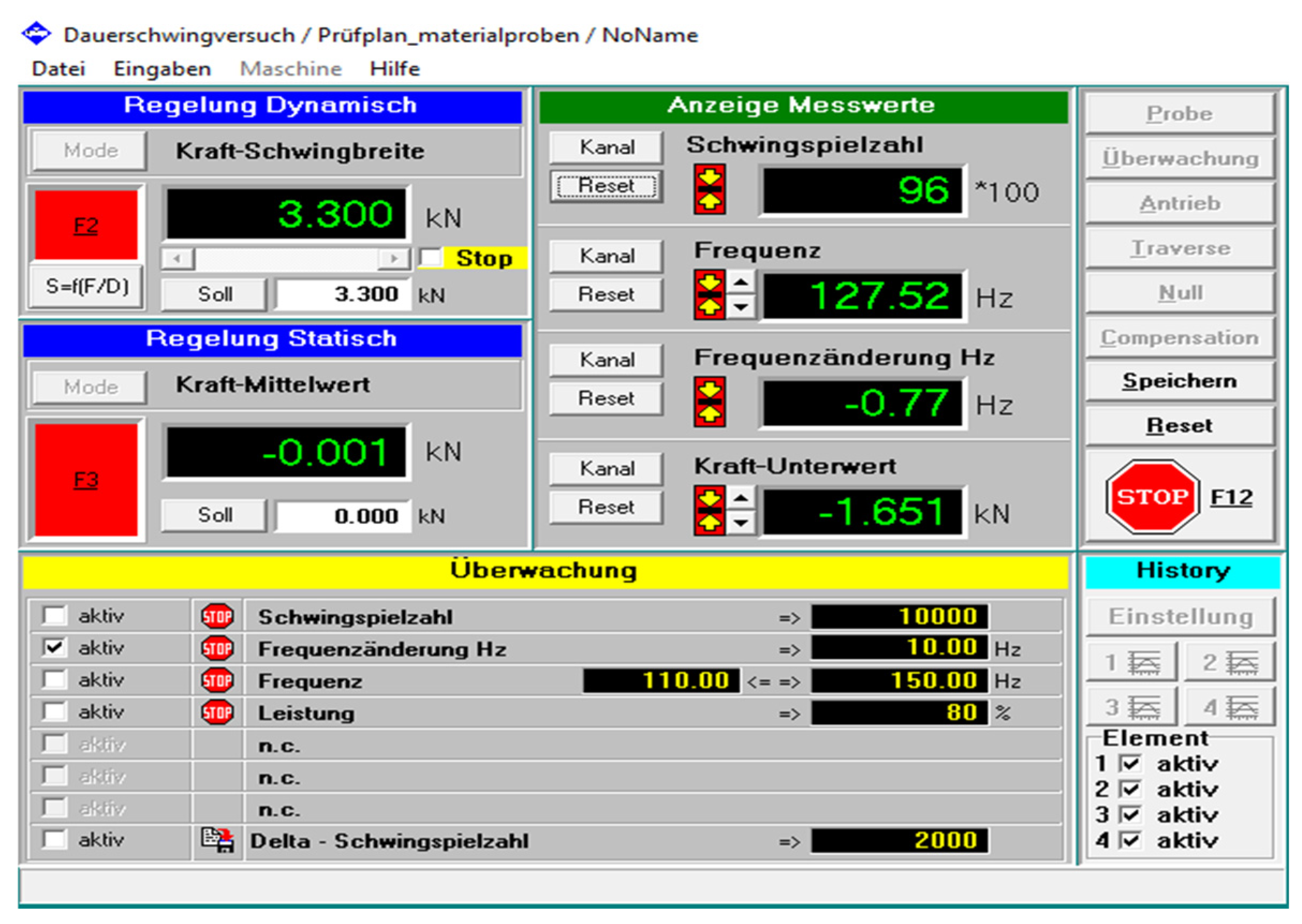
M= 1030*32= 32960 Nm
F= 3.3 kN
Thirteen samples were tested. Initially, the fatigue test was performed on 3 reference samples that broke after a certain number of cycles. Based on this result, we selected several cycles for each of the 10 additional specimens to evaluate their behaviour at different cycle intervals.
The Table 12 presents the evolution of frequency until failure, highlighting the results of tests conducted on samples 01, 02, and 03. These tests indicated a decrease in frequency, reaching a value of 22 Hz at the moment of failure. However, in all cases, the cracking of the samples occurs prior to this moment. The decrease in frequency can be correlated with the onset of the material’s cracking process. The table shows that the frequency changes for the three samples occurred alongside a decrease of 0.02 Hz, suggesting the beginning of structural deterioration.
Figure 25 shows the failure diagram with the frequency variation and the maximum number of stress cycles. It can be observed that the frequency remains constant up to 540207 cycles, indicating that the material does not show significant damage, after which a slow decrease in frequency begins, signalling the appearance of the first microcracks in the material. These microcracks begin to affect the stiffness of the material. After 965144 cycles, the frequency continues to decrease, indicating a sharp and imminent deterioration of the material. At this stage, the microcracks have expanded significantly and have considerably affected the material structure. Eventually, the material completely failed at a total of 1630529 cycles, and the final frequency recorded a significantly low value.
Figure 26 shows the oxidized sample tested to failure. Like the hardened and tempered sample, it shows a visible crack without requiring CT inspection the Figure 27a illustrates the frontal view of the specimen following a fatigue load of 1630529 cycles and Figure 27 b illustrates upper surface of the specimen.
The fatigue crack was initiated in the upper region of the radius, originating from a machining defect. Its progression is notable for its linear trajectory, with minimal branching or deviation observed. The crack length on the frontal surface of the specimen, measured from its edge, is documented as 4489 µm, corresponding to approximately one-third of the specimen’s total width
Figure 26.
Oxidized sample after breaking test.
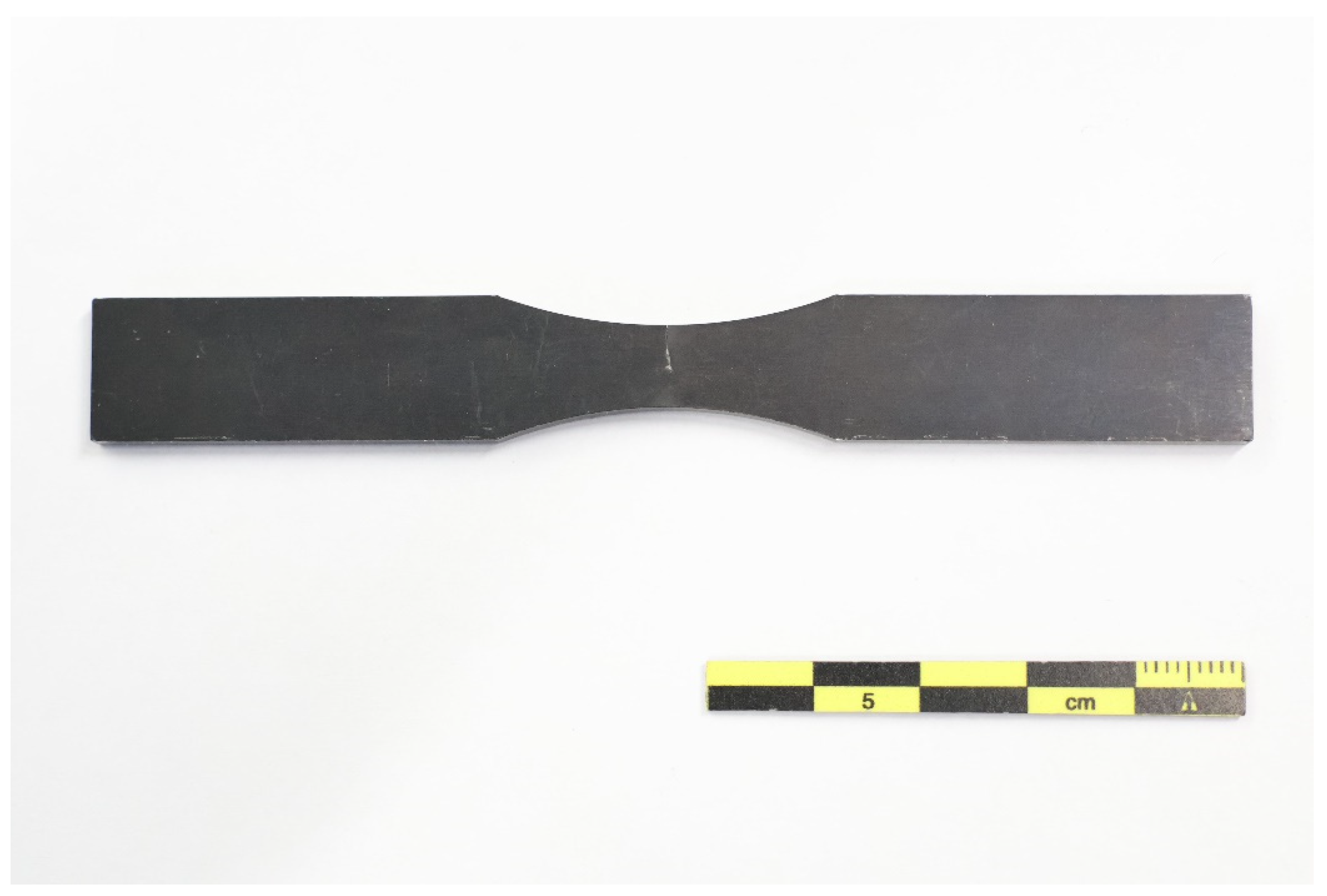
Figure 27.
a) The fatigue crack on the front side of specimen 01 after 1630529 cycles und b) upper surface of the specimen: the crack length 4489 µm.
Figure 27.
a) The fatigue crack on the front side of specimen 01 after 1630529 cycles und b) upper surface of the specimen: the crack length 4489 µm.
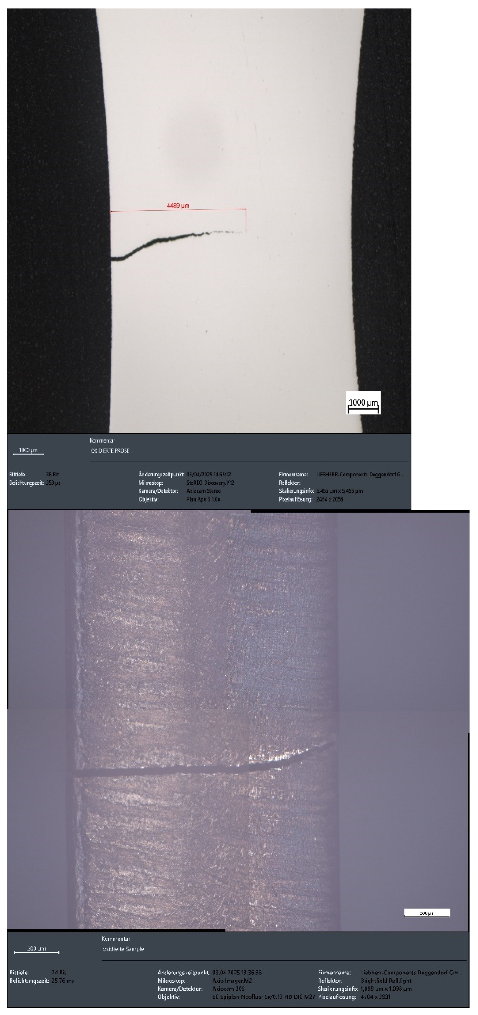
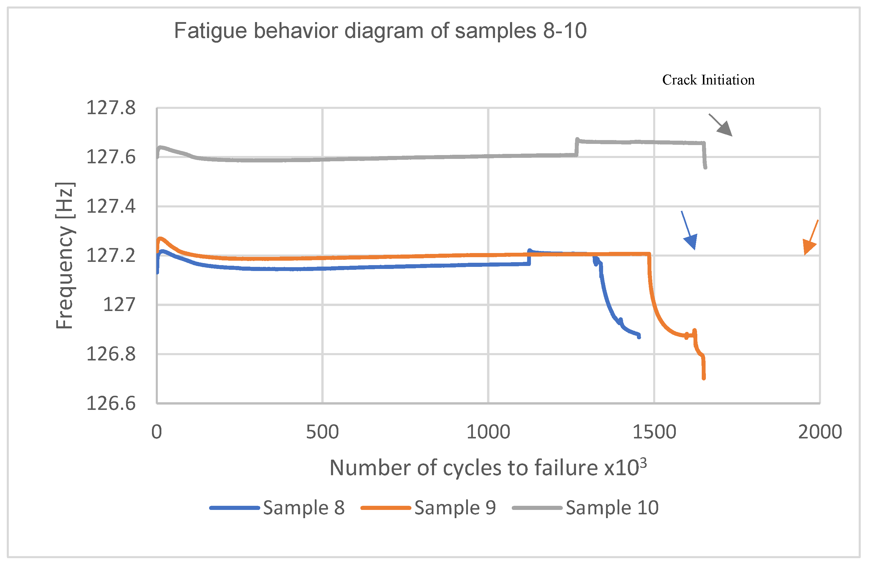
Table 13 shows the number of cycles set for each specimen of the 10 additional specimens and the frequency changes that occurred during the experiment, Figure 28 shows a diagram of the superposition of the 7 curves for the fatigue behaviour of the specimens thermochemically treated by oxidation and which showed no frequency changes, and Figure 29 shows samples 8, 9 and 10 for which a considerable decrease in frequency with 0,6 Hz was observed.
No frequency change was observed during the testing for samples 1 through 7. This indicates that the material exhibited no microcracking, thus demonstrating uniform strength and stable structural integrity under cyclic stresses.
Samples 8, 9 and 10 indicate that after the material develops microcracks, it can still withstand cyclic loading.
Table 13.
Results obtained after fatigue testing with a predetermined number of cycles.
| No. of sample | No. of cycles | Initial frequency [Hz] | Final frequency [Hz] |
|---|---|---|---|
| 1 | 165.000 | 127.08 | 127.08 |
| 2 | 330.000 | 127.24 | 127.24 |
| 3 | 495.000 | 126.97 | 126.97 |
| 4 | 660.000 | 127.39 | 127.39 |
| 5 | 825.000 | 127.18 | 127.18 |
| 6 | 990.000 | 127.19 | 127.19 |
| 7 | 1.155.000 | 127.18 | 127.18 |
| 8 | 1.320.000 | 127.20 | 126.86 |
| 9 | 1.649.762 | 127.21 | 126.70 |
| 10 | 1.654.319 | 127.60 | 126.50 |
Figure 28.
Fatigue behaviour diagram of specimens 1-7 thermochemically treated by oxidation and subjected to fatigue with a predetermined number of cycles.
Figure 28.
Fatigue behaviour diagram of specimens 1-7 thermochemically treated by oxidation and subjected to fatigue with a predetermined number of cycles.
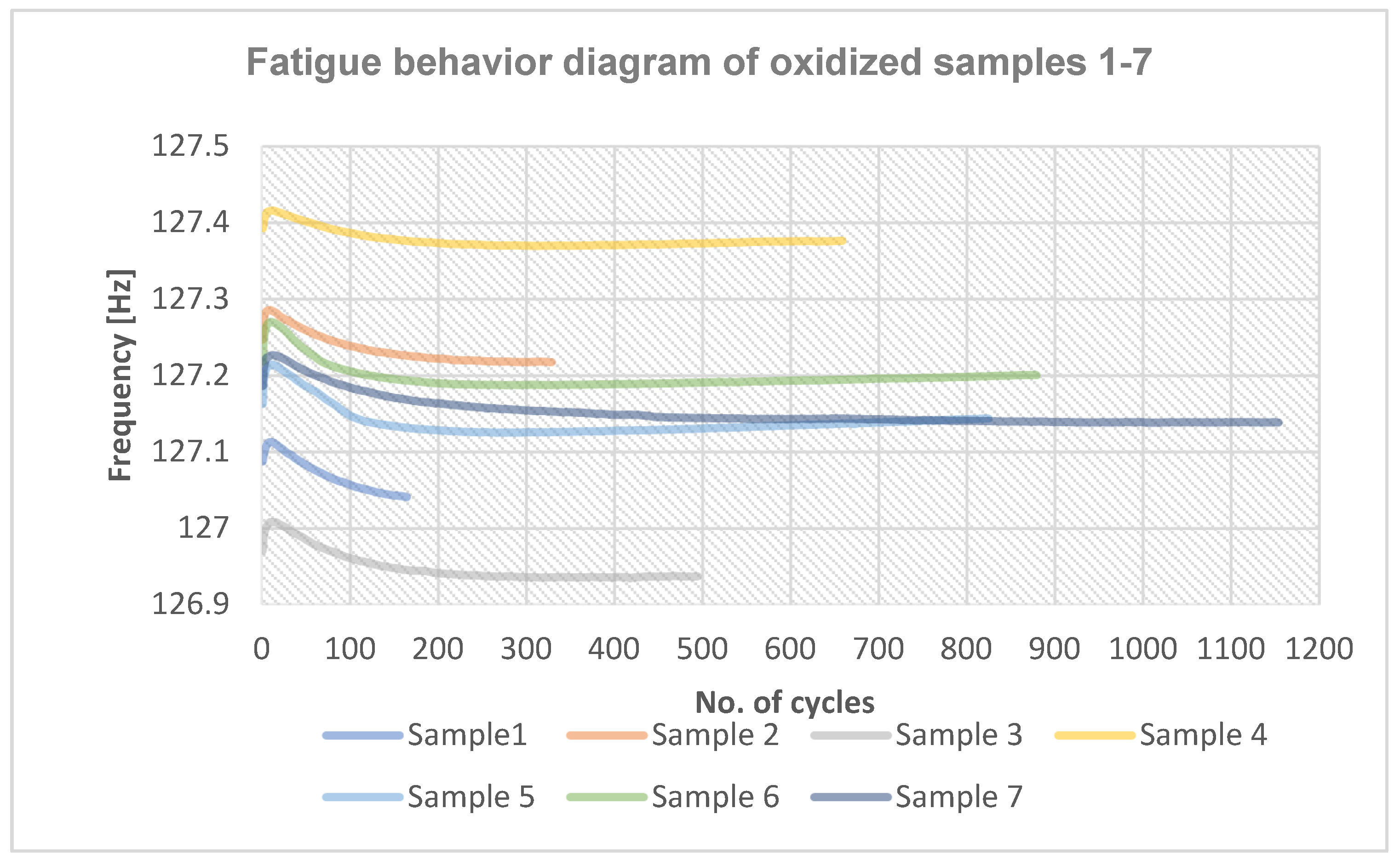
Figure 29.
Fatigue behaviour diagram of specimens 8-10 thermochemically treated by oxidation and subjected to fatigue with a predetermined number of cycles.
Figure 29.
Fatigue behaviour diagram of specimens 8-10 thermochemically treated by oxidation and subjected to fatigue with a predetermined number of cycles.
4.6. Computed Tomography (CT) Analysis of the Oxidized Sample After Fatigue Testing
To verify the hypothesis that the frequency drop indicates the appearance of microcracks in the material, we conducted a computed tomography (CT) inspection. This method allowed us to analyze the internal structure of the specimen in detail and confirm the presence of microcracks, thus validating our hypothesis.
Samples 8 in which a decrease in frequency was observed were tested with liquid penetrant and tomographic inspection. The liquid penetrant analysis showed the presence of a microcrack on one of the sides. On the other hand, computed tomography (CT) allowed detailed detection of the internal microcracks, providing additional information about their size and exact localization in the entire volume of the material, Figure 30
The sample initially presents a crack in the radius area, which subsequently extends to the frontal surface. The crack size in the radius area is 1.33 mm, while on the frontal surface the crack measures 1.35 mm. This evolution of the crack indicates a propagation of the defect from the radius area to the frontal surface, thus highlighting the critical points of the material.
5. Conclusions
- The samples thermally treated as delivered had a fatigue life of about 205700 cycles, with rapid microcrack formation and a short life after microcrack formation. Microcrack formation was observed in the material at 97% of total life. After microcracking, the material deteriorates rapidly. Therefore, it can be concluded that the material showed high fatigue resistance up to 140.000 cycles, being able to withstand repeated cyclic loads without losing its integrity.
- The samples thermochemically treated by oxidation exhibited a significantly longer life, reaching approximately 1628681 cycles to failure, and cracks formed at an early stage under cyclic stress. However, the subsequent growth of microcracks lasted longer, occupying most of the life, which resulted in improved performance compared to the thermally treated samples.
- For the oxidized sample no. 8, which had a life of 1320000 cycles, a change in frequency is observed at 1121000 cycles. For sample 9, which had a life of 1649762 cycles, a change in frequency is observed at 1484718 cycles, and for sample 10, which had a life of 1654319 cycles, a change in frequency is observed at 1265412 cycles. These observations indicate that microcracks are formed at approx. 80% of life, but the material can still withstand cyclic loading before failing.
Impact of Treatments:
- Thermal treatments improved the initial fatigue resistance and homogenized the material structure, reducing stress concentration and crack propagation.
- Thermochemical treatment by oxidation gave the best results in terms of fatigue life and resistance to microcrack propagation due to the oxide layer formed on the material surface. These findings highlight the advantages of thermochemical oxidation treatments in improving the durability and reliability of C60 steel.
- The connection between oxidized specimens with a longer duration until failure, despite early crack initiation, and the specimens with increased hardness and shorter lifespan can be explained as follows:
Oxidized Specimens:
- In the case of oxidized specimens, early crack initiation can occur due to surface defects or the weakening effects of oxidation.
- However, the oxide layer formed on the surface acts as a protective barrier, slowing down the crack’s propagation. This can extend the overall lifespan of the specimen by reducing local stress concentrations. Over a specific stress range,oxidation positively impacts fatigue life, effectively balancing the detrimental effects of early crack initiation
- The significant decrease in the core hardness of the oxidized samples, compared to the tempered delivery condition, is due to the temperature and oxidation time, which led to an increase in fatigue resistance.
Improved Specimens
- As shown in the fracture diagram for the improved specimens, the already formed cracks propagate more rapidly. This phenomenon can be explained by the association of increased hardness of the improved material with increased brittleness.
- There is a trade-off between crack initiation resistance and crack propagation resistance. Oxidized specimens, while more prone to early crack initiation due to surface oxidation, benefit from a slower crack growth due to the protective nature of the oxide layer. On the other hand, harder specimens resist crack initiation better but experience rapid crack propagation, leading to a shorter lifespan overall.
Microstructural Analysis:
- Microstructural changes induced by thermal and thermochemical treatments were correlated with improvements in fatigue resistance. The oxide layer formed on the thermochemically treated material contributed to reduced crack propagation and increased material durability.
Recommendations:
- The application of thermochemical oxidation treatment is recommended to achieve superior fatigue resistance and longer material life. It is also essential to monitor the frequency of stress cycling to detect and prevent microcracking at early stages.
- In conclusion, thermochemical treatment by oxidation has shown the best results in terms of fatigue life and resistance to microcrack evolution, and knowledge of the timing of their occurrence allows the tests to be adjusted to better reflect the actual conditions of use of the materials. These findings contribute to the development of stronger and more durable materials for industrial applications.
- Professor Emeritus Cornel SAMOILĂ, EngD guided me as scientific supervisor.
- Director Simon Oreskovic of Zerlos Zerspanung, Germany, helped me in the realization of the specimens.
- Eng. Joachim Reese of the heat treatment company “Härterei Reese Brackenheim”, Germany, carried out the thermochemical oxidation treatment of the specimens.
- Mr. Uwe Leuteritz, EngD, Mr. Matthias Zech and Mr. Johannes Dallmeier of Liebherr Deggendorf, Germany, made the fatigue test possible by improving the machine.
Acknowledgments
The completion of these experiments was possible with the help of important collaborators. We received technical assistance and support from the following individuals and organizations:.
Competing interests
I: the undersigned Tudorache (married Nistor), hereby declare that there are no competing interests influencing the work presented in this paper. I have no financial or personal relationship with any other person or organization that could improperly influence my work.
References
- CHENG, W - Micromechanics Modelling of Crack Initiation Under Contact Fatigue, Journal of Tribology, vol. 116, January 1994. [CrossRef]
- Agrawal, A.; Deshpande, P. D.; Cecen, A.; Basavarsu, G. P.; Choudhary, A. N.; Kalidindi, S. R. Exploration of data science techniques to predict fatigue strength of steel from composition and processing parameters. Integr. Mater. Manuf. Innov. 2014, 3, 90–108. [CrossRef] 69. He, L.; Wang, Z. L.; Akebono, H.; Sugeta. [CrossRef]
- Cui, W.C. A state-of-the-art review on fatigue life prediction methods for metal structures. J. Mar. Sci. Technol. 2002, 7, 43–56. [Google Scholar] [CrossRef]
- Oliviu, R., Teodorescu M., Lascu N., Oboseala metalelor - Baze de calcul (Metal fatigue - Calculation bases), vol. 1, Tehnica Publishing House, Bucharest, 1992.
- Dumitru I., Faur N.: Bazele teoretice în Oboseala Materialelor, Mecanica Ruperii, Materiale compozite şi Metode Numerice (Theoretical foundations in material fatigue, fracture mechanics, composite materials and numerical methods) -1997.
- Doebling, S.W.; Farrar, C.R.; Prime, M.B.; Doebling, S.W.; Farrar, C.R.; Prime, M.B. A Summary Review of Vibration-Based Damage Identification Methods. Shock Vib. Digest. 1998, 30, 91–105. [Google Scholar] [CrossRef]
- Zai, B.A.; Khan, M.A.; Khan, S.Z.; Asif, M.; Khan, K.A.; Saquib, A.N.; Mansoor, A.; Shahzad, M.; Mujtaba, A. Prediction of crack depth and fatigue life of an acrylonitrile butadiene styrene cantilever beam using dynamic response. J. Test. Eval. 2020, 48, 1520–1536. [Google Scholar] [CrossRef]
- Vamvoudakis-Stefanou, K.J.; Sakellariou, J.S.; Fassois, S.D. Vibration-based damage detection for a population of nomi-nally identical structures: Unsupervised Multiple Model (MM) statistical time series type methods. Mech. Syst. Signal Process. 2018, 111, 149–171. [Google Scholar] [CrossRef]
- Zhipeng Chong, Chaanghao Wang, Qianwei Wang, Xiaopeng Cheng, Chao Wang, Xingping Liu, Bing Wang, Yuefei Zhang, Ruzhi Wang-High- Precision identification and classification of alloy fatigue microcracks trough deep learning ans in-situ SEM-Computational Material Science, Volume 252, April 2025. [CrossRef]
- Xiangyun Long, Hongyu Ji, Jinkang Liu, Xiaogang Wang, Chao Jiang-MT-CrackNet: A multi task deep learning framewocrk for automatic in-situ fatigue micro-crack detection and quantification-International Journal of Fatigue, Volume 190, January 2025. [CrossRef]
- Reifsneider, K. L., Fatigue of composite materials, Series 4, Elsevier Science Publishers, 1991. ISBN: 0-444-42525-X.
- Babibsky, T.; Kubena, T.; Sulak, I.; Krumi, T.; Tobias, J.; Polak, J. Surface relief evolution and fatigue crack initiation in Rene 41 superalloy cycled at room temperature. Mater. Sci. Eng. 2021, 819, 141520. [Google Scholar] [CrossRef]
- Kwon, H.; Barlat, F.; Lee, M.; Chung, Y.; Uhm, S. Influence of Tempering Temperature on Low Cycle Fatigue of High Strength Steel. ISIJ Int. 2014, 54, 979–984. [Google Scholar] [CrossRef]
- Shiyong, L.; Deyi, L.; Shicheng, L. Effect of heat treatment on the fatigue resistance of spring steel 60Si2CrVA. Met. Sci. Heat Treat. 2010, 52, 57. [Google Scholar] [CrossRef]
- R.K.Rai:The role of cyclic oxidation on low cycle fatigue crack initiation growth behaviour of a Ni-based superalloy- Materials Chemistry and Physics, Volume 32,15 February 2025.
- S.Cruchley, H.Y. Li, H.E. Evans, P. Bowen, D.J. Child and M.C. Hardy-The Role of Oxidation Damage in Fatigue Crack Initiation of an Advanced Ni-based Superalloy, International Journal of Fatigue Volume 81, December 2015, Pages 265-274. [CrossRef]
- Mayer, H.; Haydn, W.; Schuller, R.; Issler, S.; Furtner, B.; Bacher-Höchst, M. Very high cycle fatigue properties of bainitic high carbon–chromium steel. Int. J. Fatigue 2009, 31, 242–249. [Google Scholar] [CrossRef]
- Kamaya, M. Observation of fatigue crack initiation and growth in stainless steel to quantity low-cycle fatigue damage for plant maintenance. EJAM E-J. Adv. Maint. 2013, 5, 155–200. [Google Scholar]
- Yang G, Wang M, Li Q, Ding R. Methodology to evaluate fatigue damage of high-speed train welded bogie frames based on on-track dynamic stress test data. Chin J Mech Eng 2019;32:1–8. [CrossRef]
- Özkara, M: Anrisslebensdauer von Stahlfeinblech, Masterthesis, Labor für Werkstoff und Fügetechnick an der Hochschule Esslingen, 2015.
- Thum, M., Özkara, M., Metzger, M., Kantop, M.: Experimentelle und rechnerische Ermittlung des Kanteneinflusses auf das Schwingfestigkeitsverhalten von Stahlfeinblech, Projektbericht, Labor für Werkstoff- und Fügetechnick an der Hochschule Esslingen, 2016.
- VDEh: Prüf- und Dokumentationscrichtlinie für die mechanischen Kernwerte von Feinblechen aus Stahl, Stahl-Eisen Prüfblatt 1240, Verein Deutscher Eisenhüttenleute, 2003.
- Radaj, D., Vorwald,M.: Ermüdungsfestigkeit, Springer-Verlag, Berlin, 2007 (3. Aflage).
- Haibach, E.: Betribfestigkeit, Springer- Verlag, Berlin, 2006 (3. Auflage).
- STAS 1963-81, - "Rezistenţa materialelor. Terminologie şi simboluri" (Strength of materials. Terminology and symbols).
- Gelu, I. Organe de Masini (Machine parts); Part I, Politehnium Publishing House: Iasi, Romania, 2010; ISBN 978-973-621-176-8.
Figure 1.
Shape and dimension of fatigue specimens [mm], under SR ISO 1099:2017.
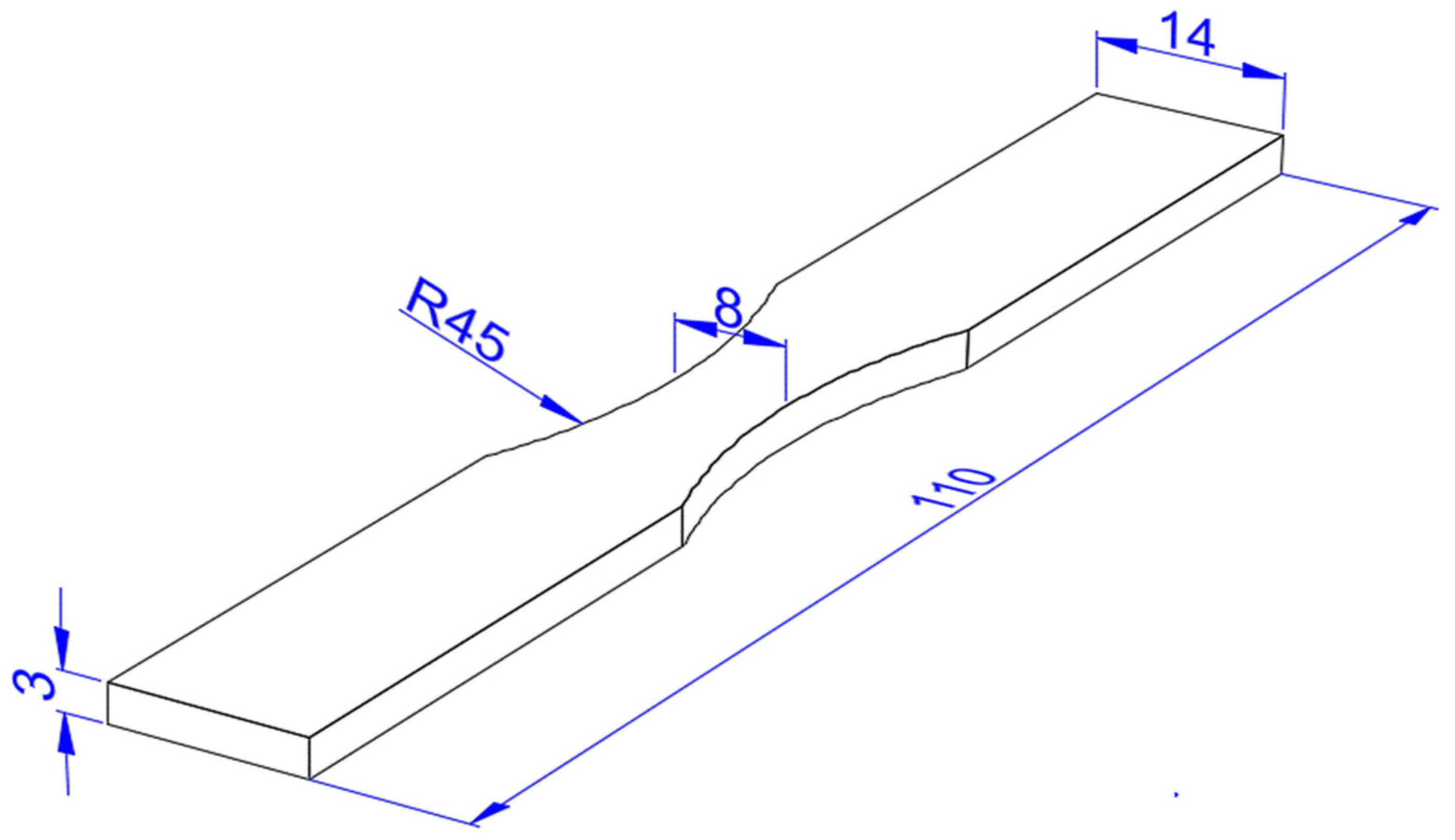
Figure 2.
Fatigue-testing machine.
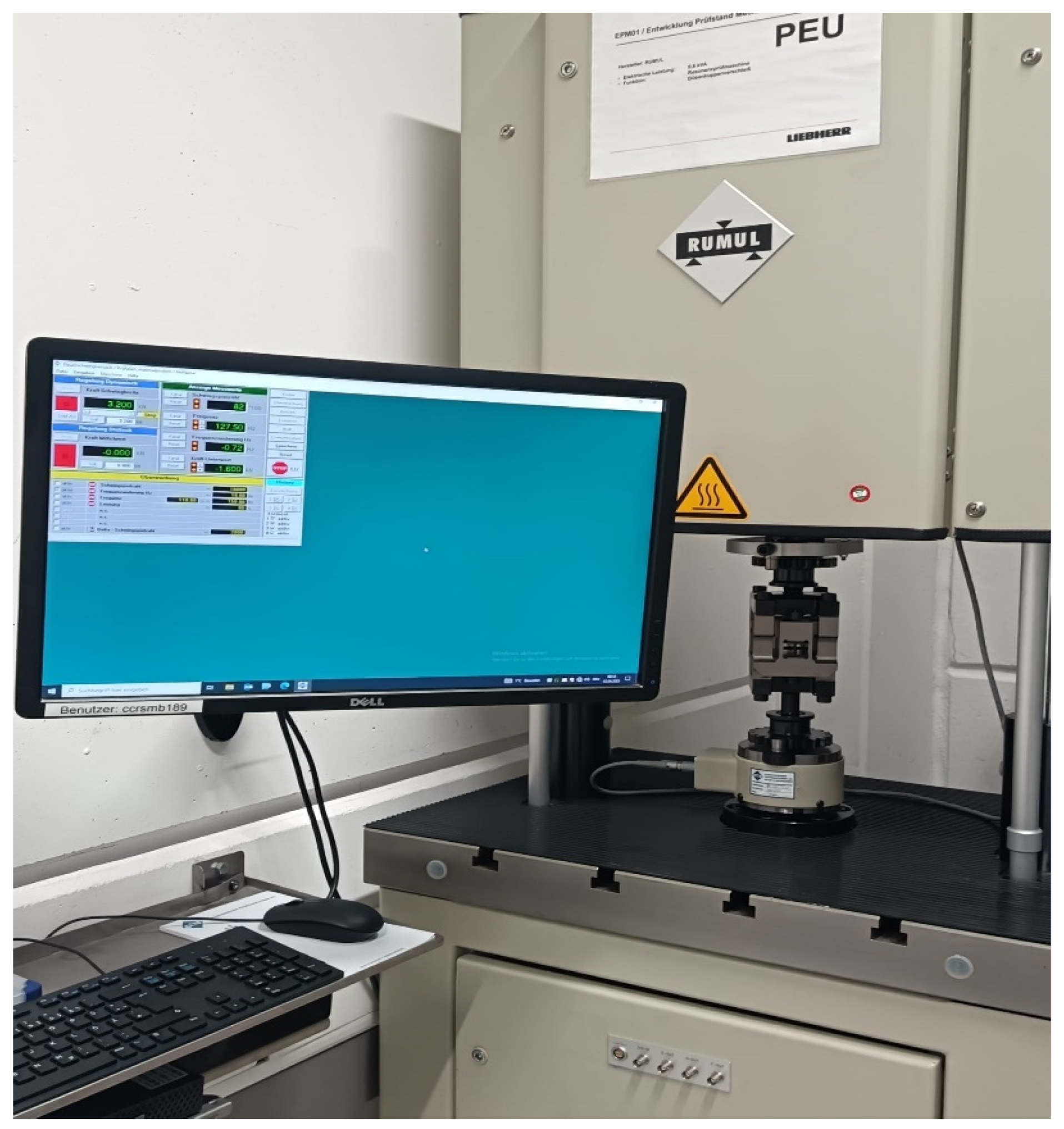
Figure 4.
Sample in delivery condition.
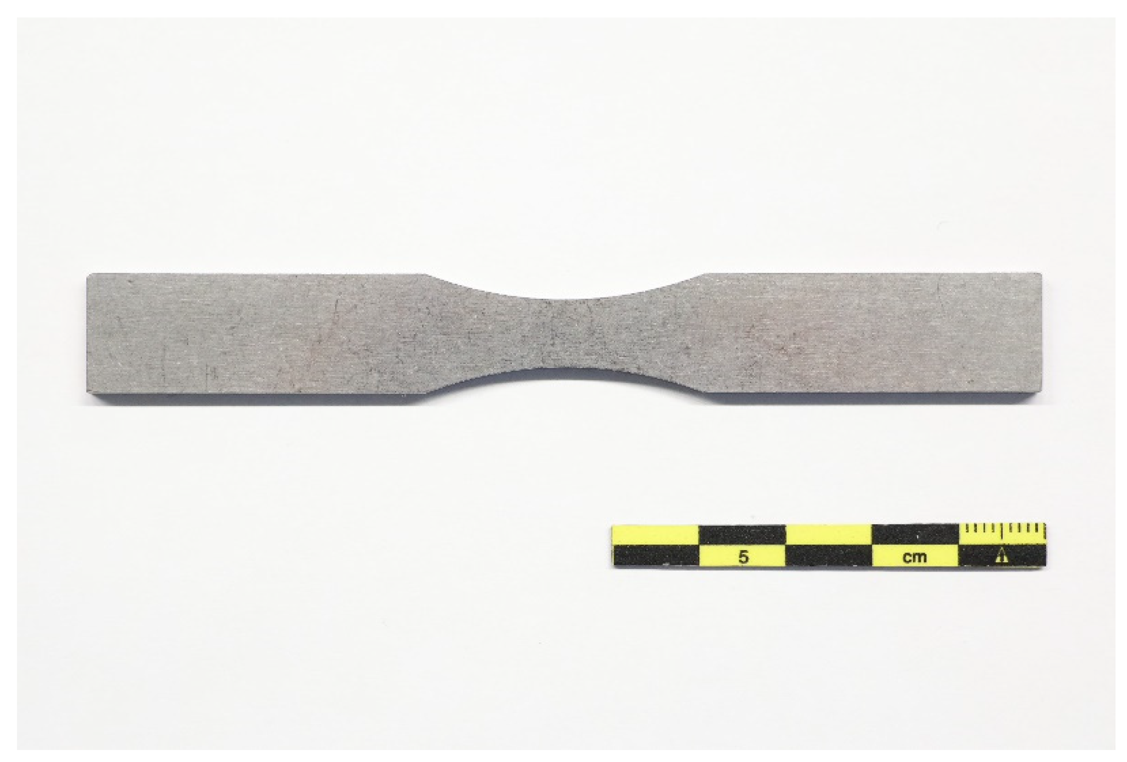
Figure 6.
Cyclogram of the oxidation process.
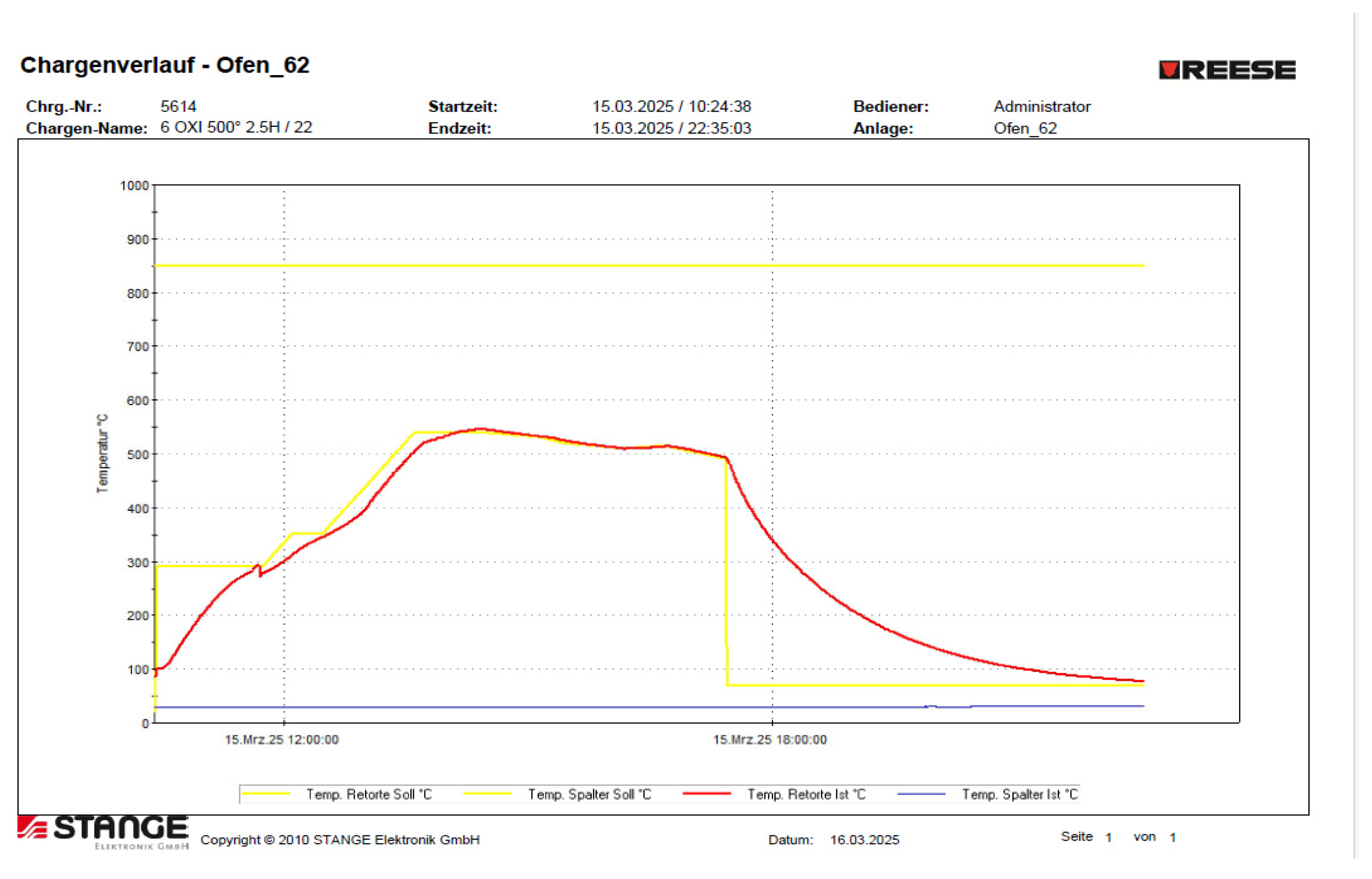
Figure 7.
Sample before oxidation.
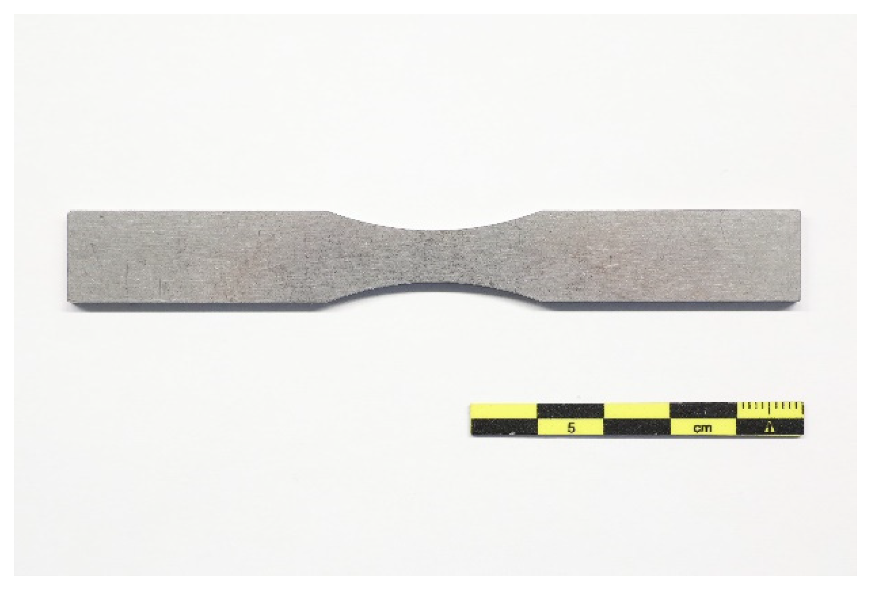
Figure 8.
Sample after oxidation.
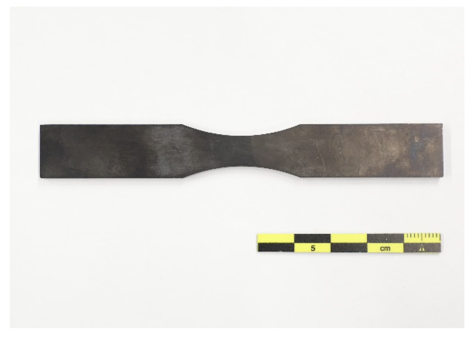
Figure 13.
Surface Profilometry of improved Specimens: Rz=0,794 µm.
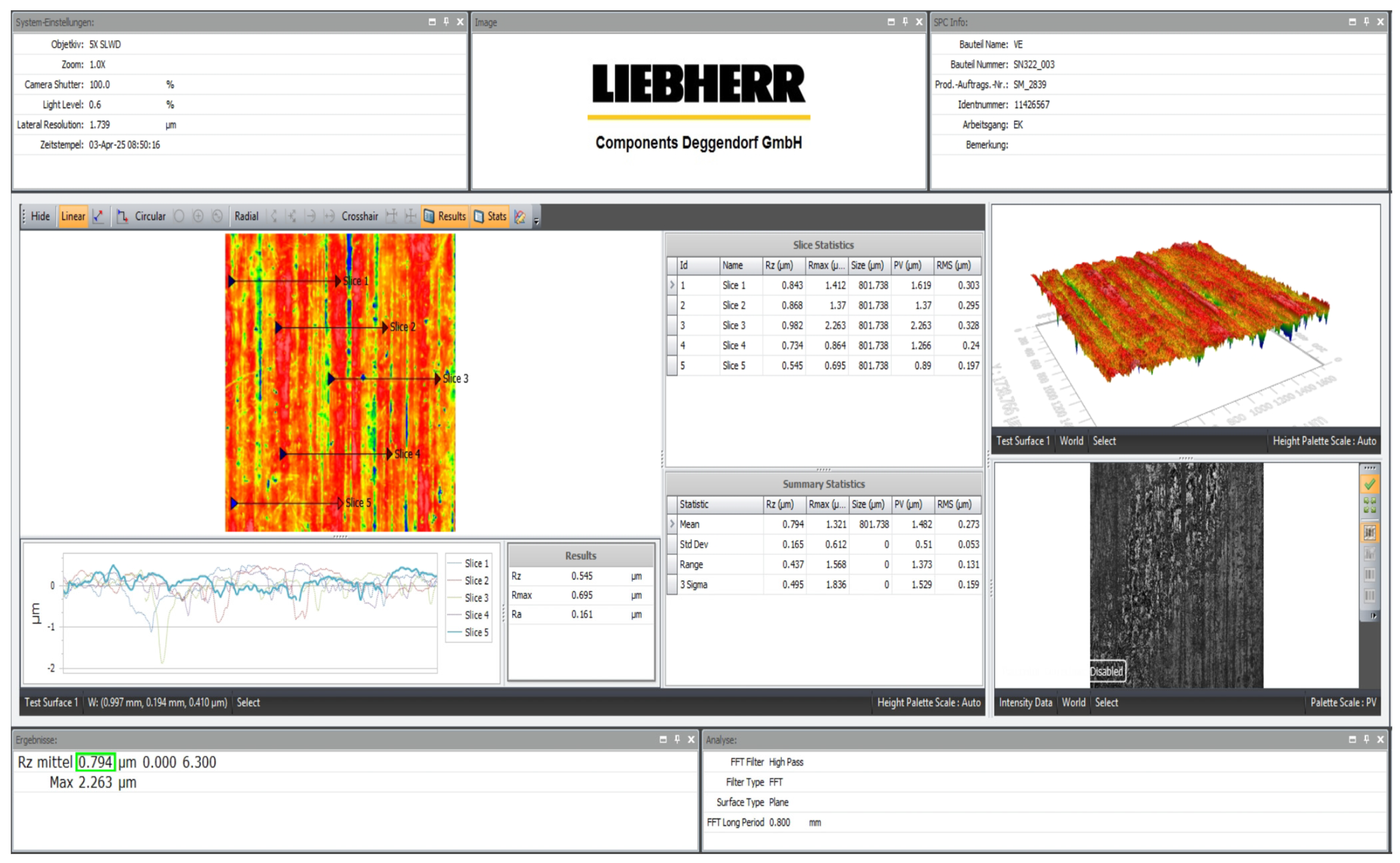
Figure 14.
Surface Profilometry of Thermochemical Oxidation Treatment specimen Rz=0,861 µm.
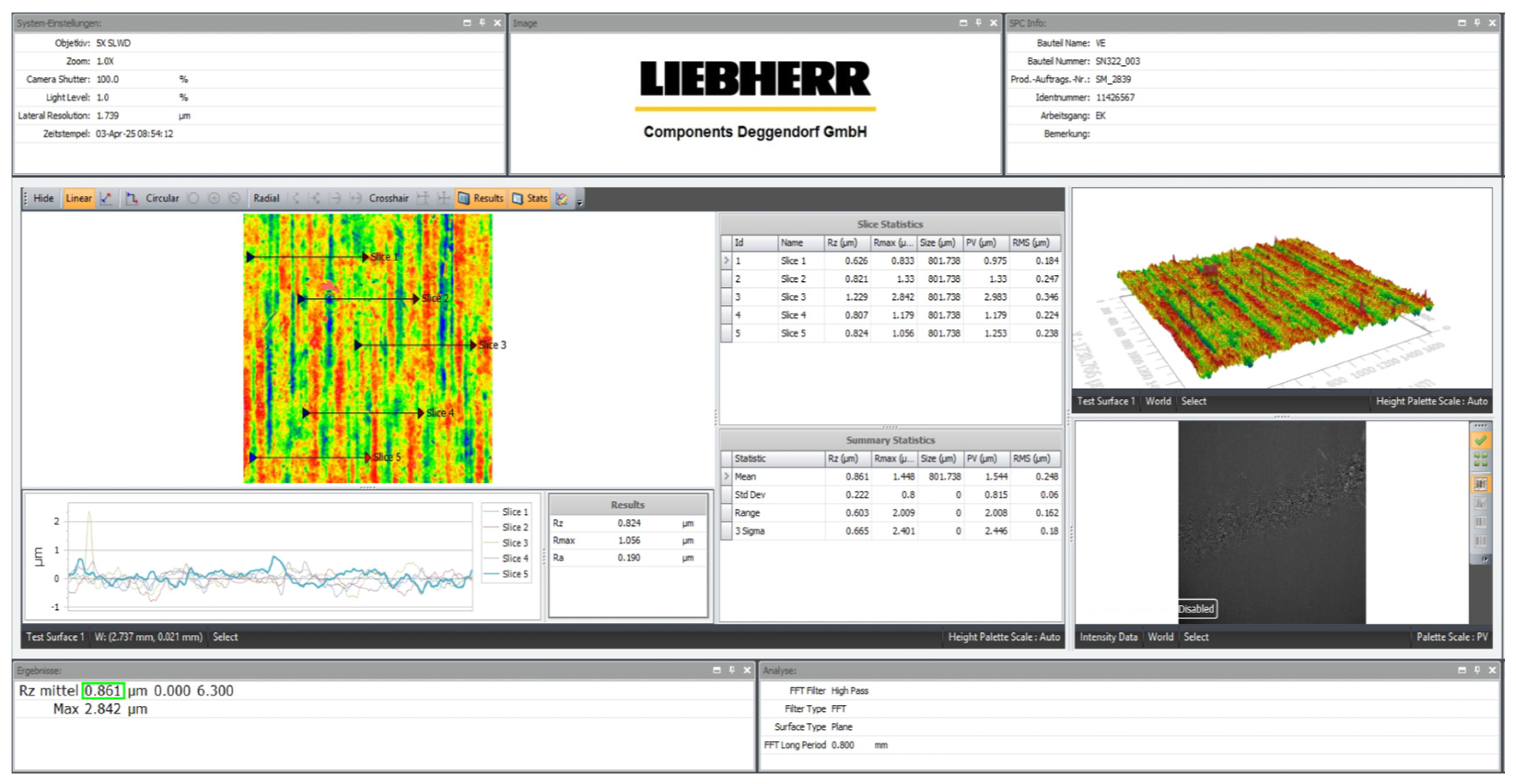
Figure 15.
Load extension diagram for hardened and tempered C60 steel.
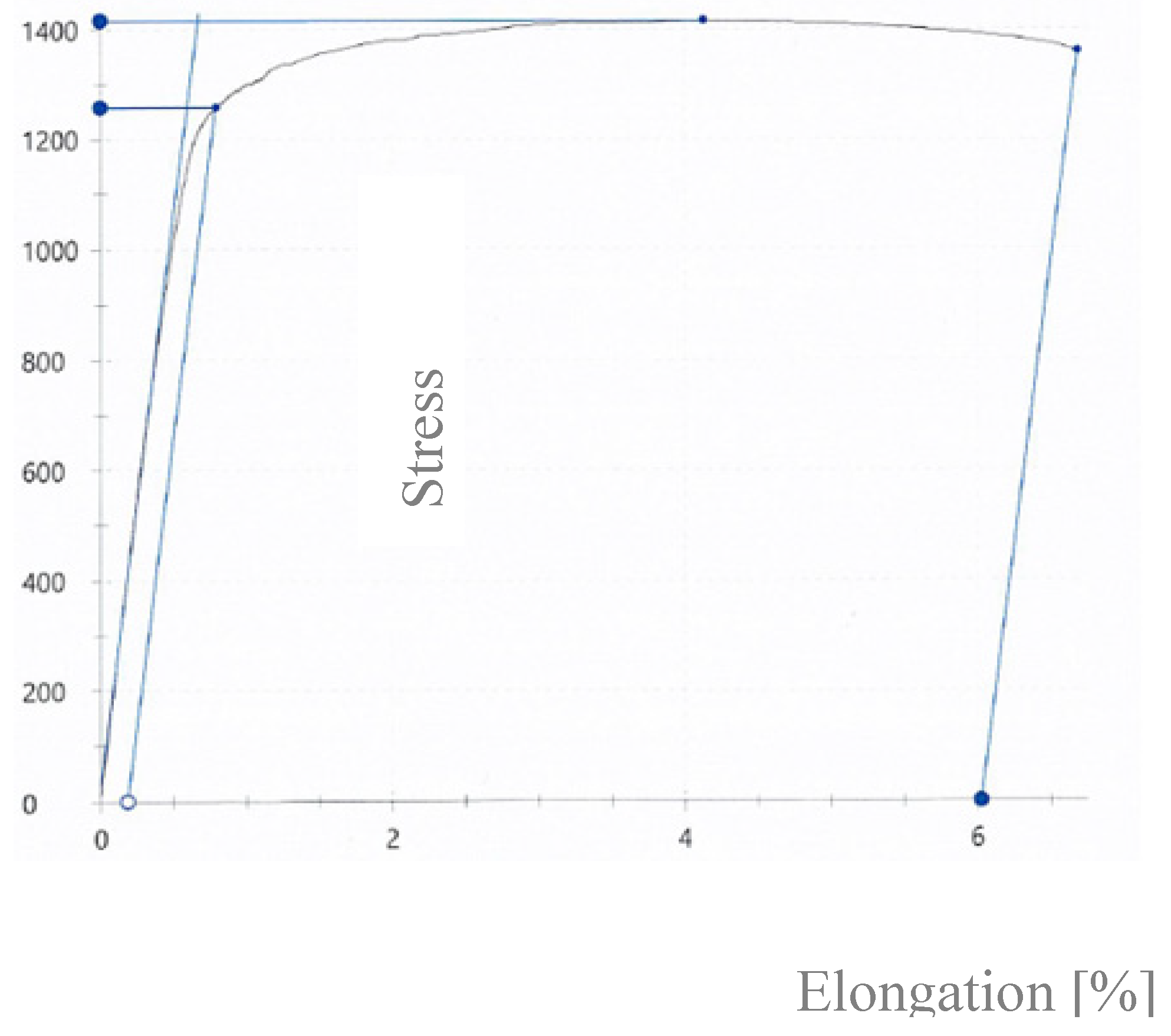
Figure 18.
Schematic representation of the evolution of the test frequency as a function of the number of cycles (Dittmann and Pätzold, 2018).
Figure 18.
Schematic representation of the evolution of the test frequency as a function of the number of cycles (Dittmann and Pätzold, 2018).
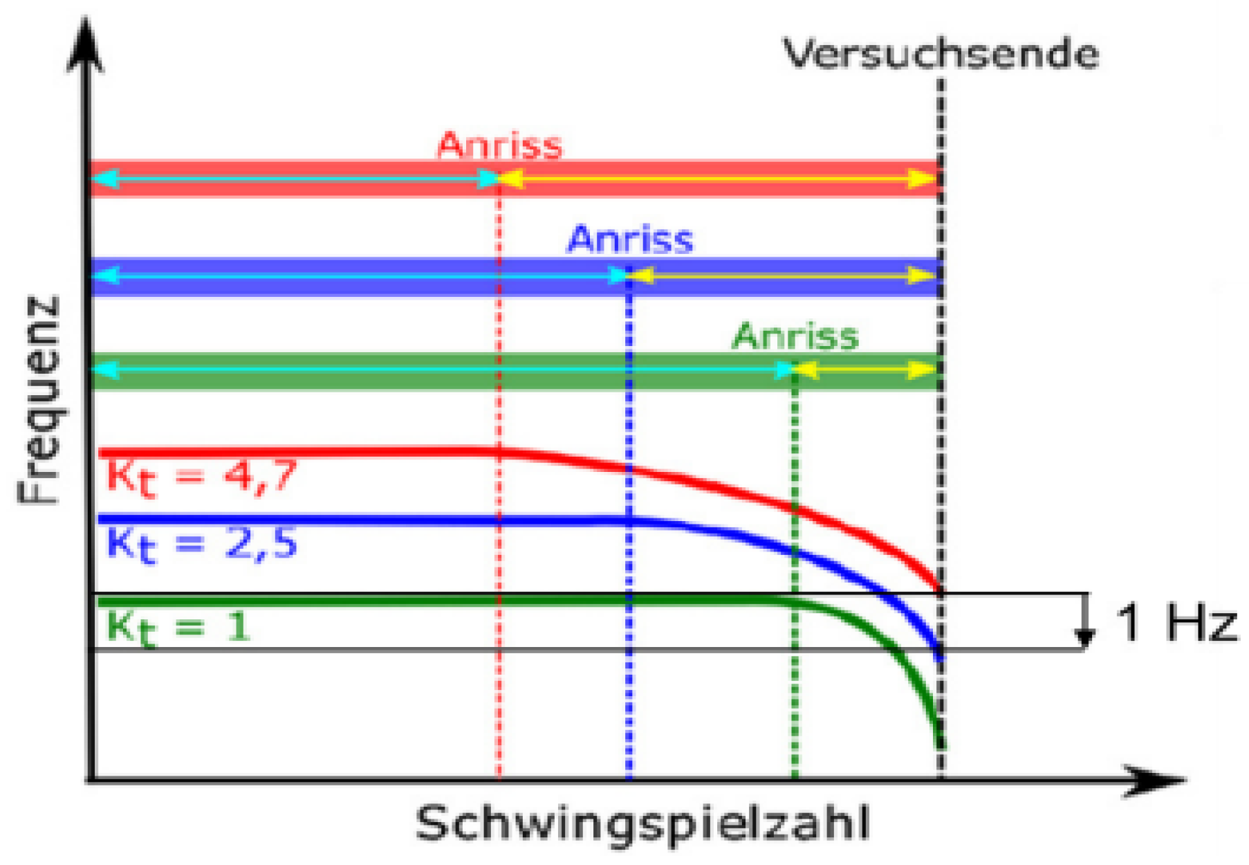
Figure 19.
Hardened and tempered sample after fatigue test.
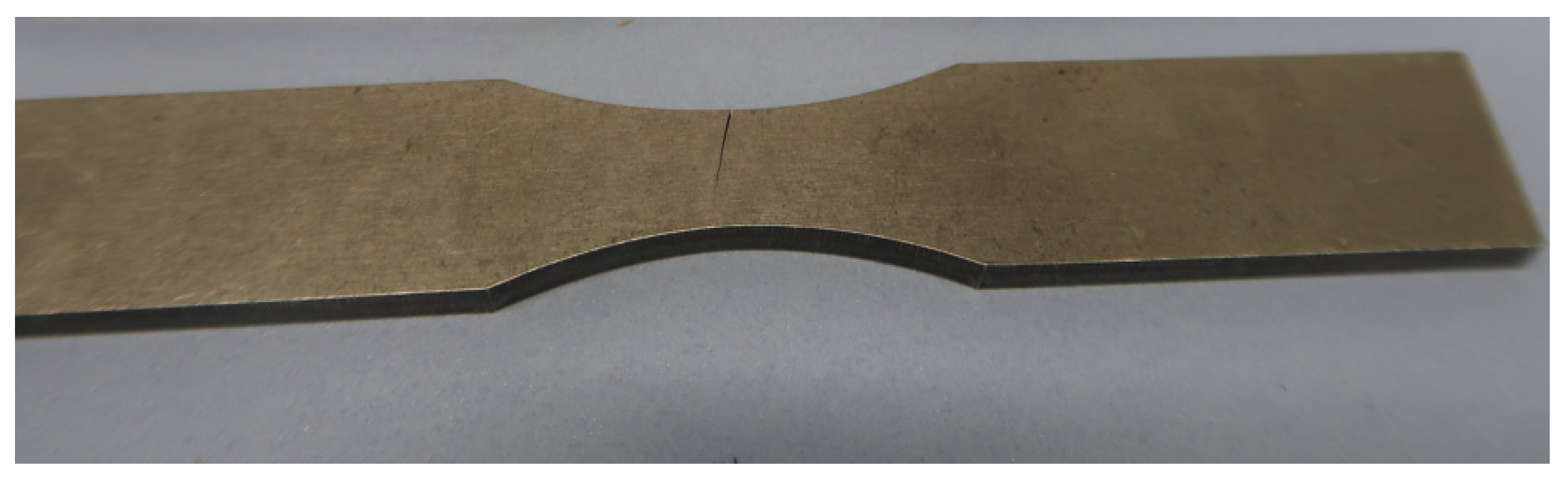
Figure 20.
a) The fatigue crack on the front side of specimen 02 after 202800 cycles [the crack length 5701 µm] und b) upper surface of the specimen.
Figure 20.
a) The fatigue crack on the front side of specimen 02 after 202800 cycles [the crack length 5701 µm] und b) upper surface of the specimen.
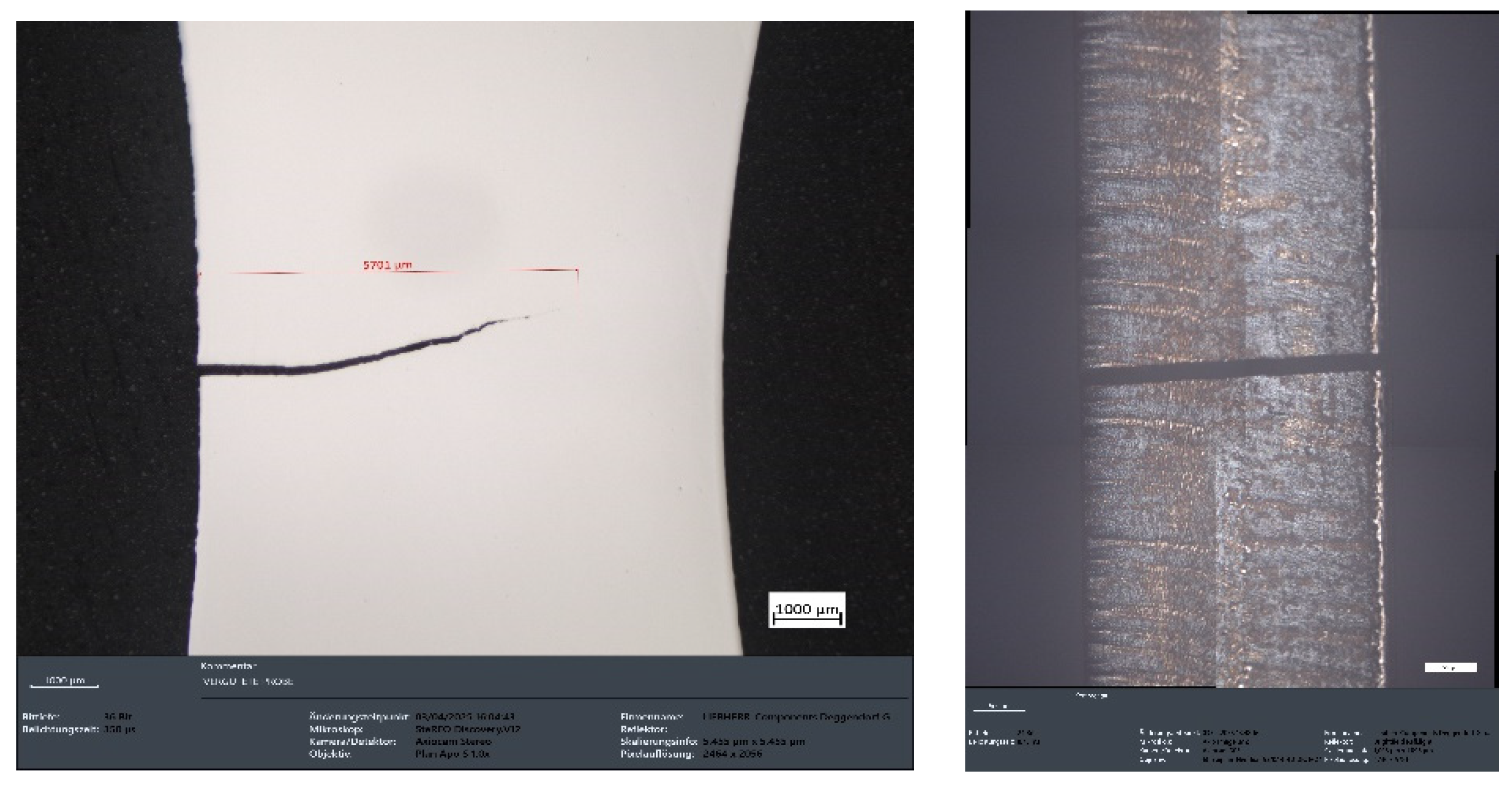
Figure 21.
Fatigue behaviour diagram for the 10 hardened and tempered samples subjected to fatigue with a predetermined number of cycles.
Figure 21.
Fatigue behaviour diagram for the 10 hardened and tempered samples subjected to fatigue with a predetermined number of cycles.
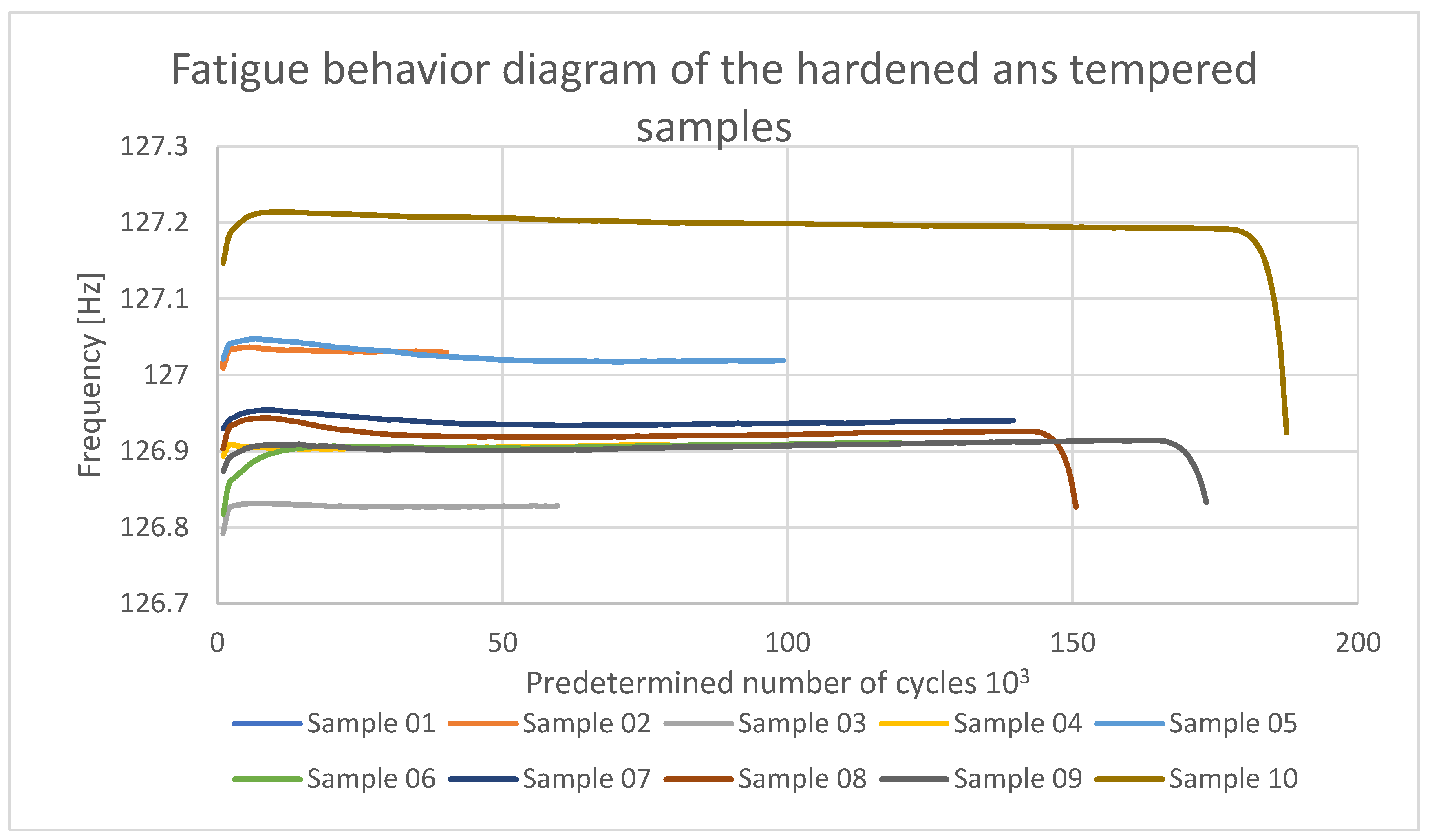
Figure 22.
Non-destructive analysis applied to hardened and tempered C60 steel, after fatigue testing: a) and b) liquid penetrant inspection and c) and d) tomographic inspection.
Figure 22.
Non-destructive analysis applied to hardened and tempered C60 steel, after fatigue testing: a) and b) liquid penetrant inspection and c) and d) tomographic inspection.
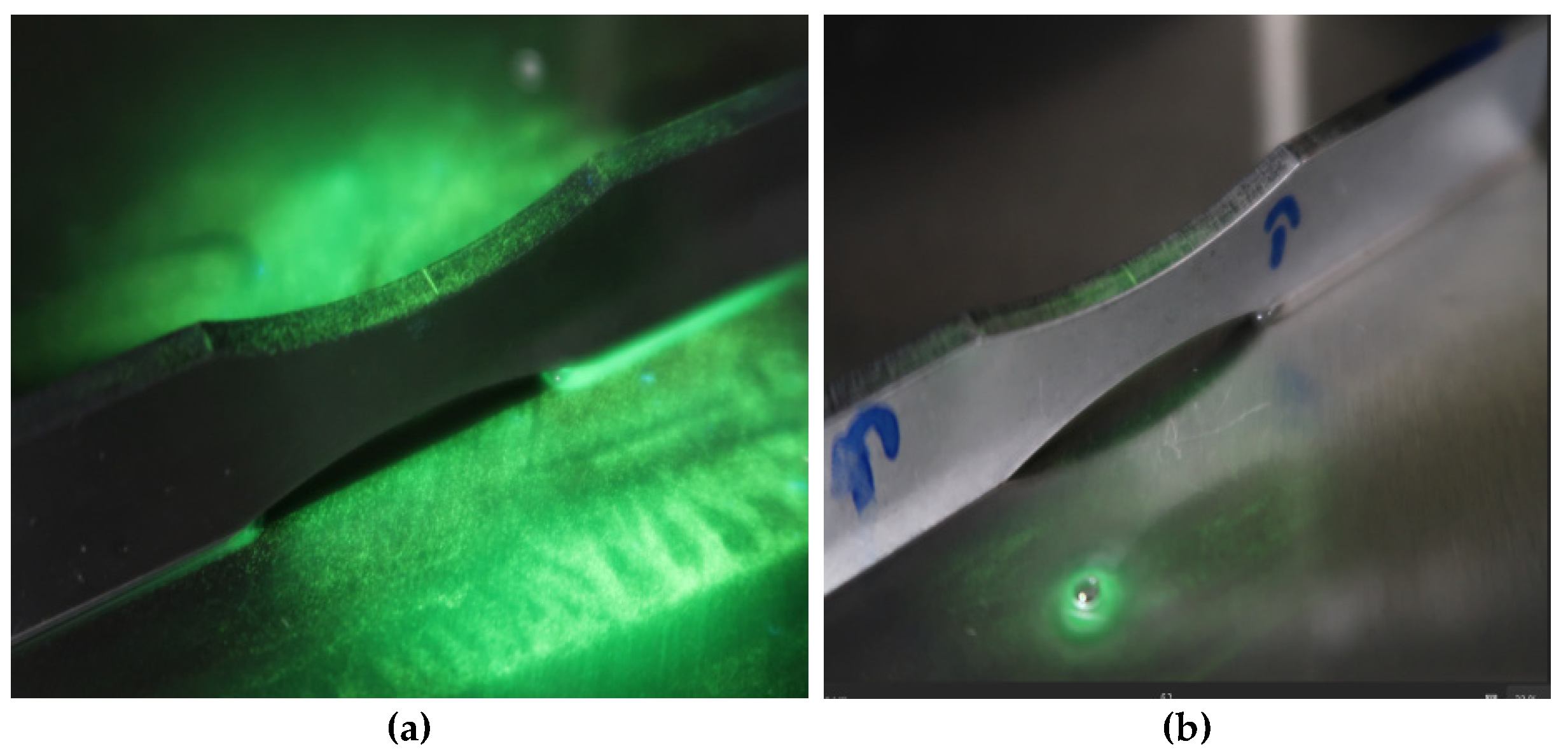
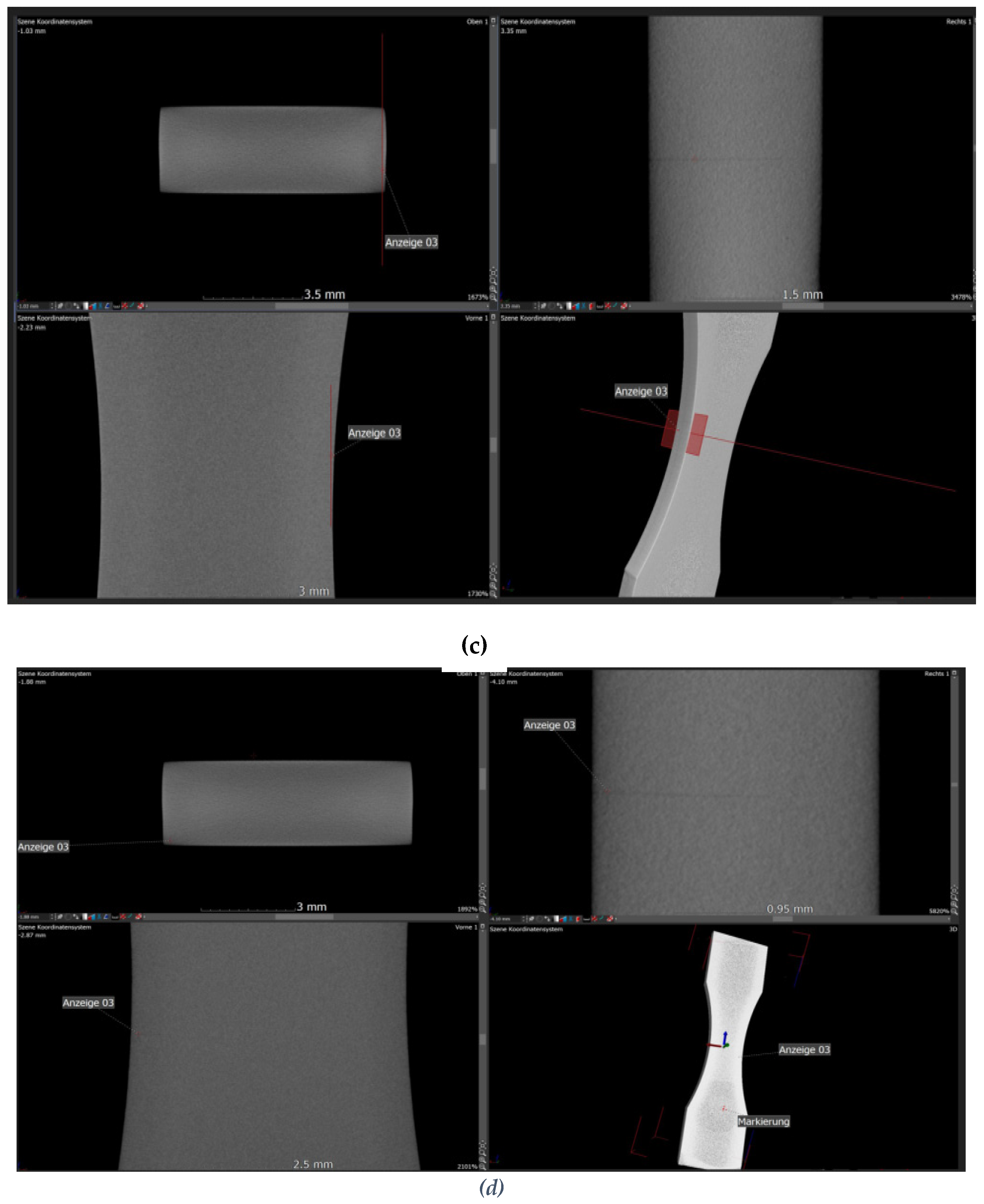
Figure 25.
Failure diagram for thermochemically oxidation-treated sample.
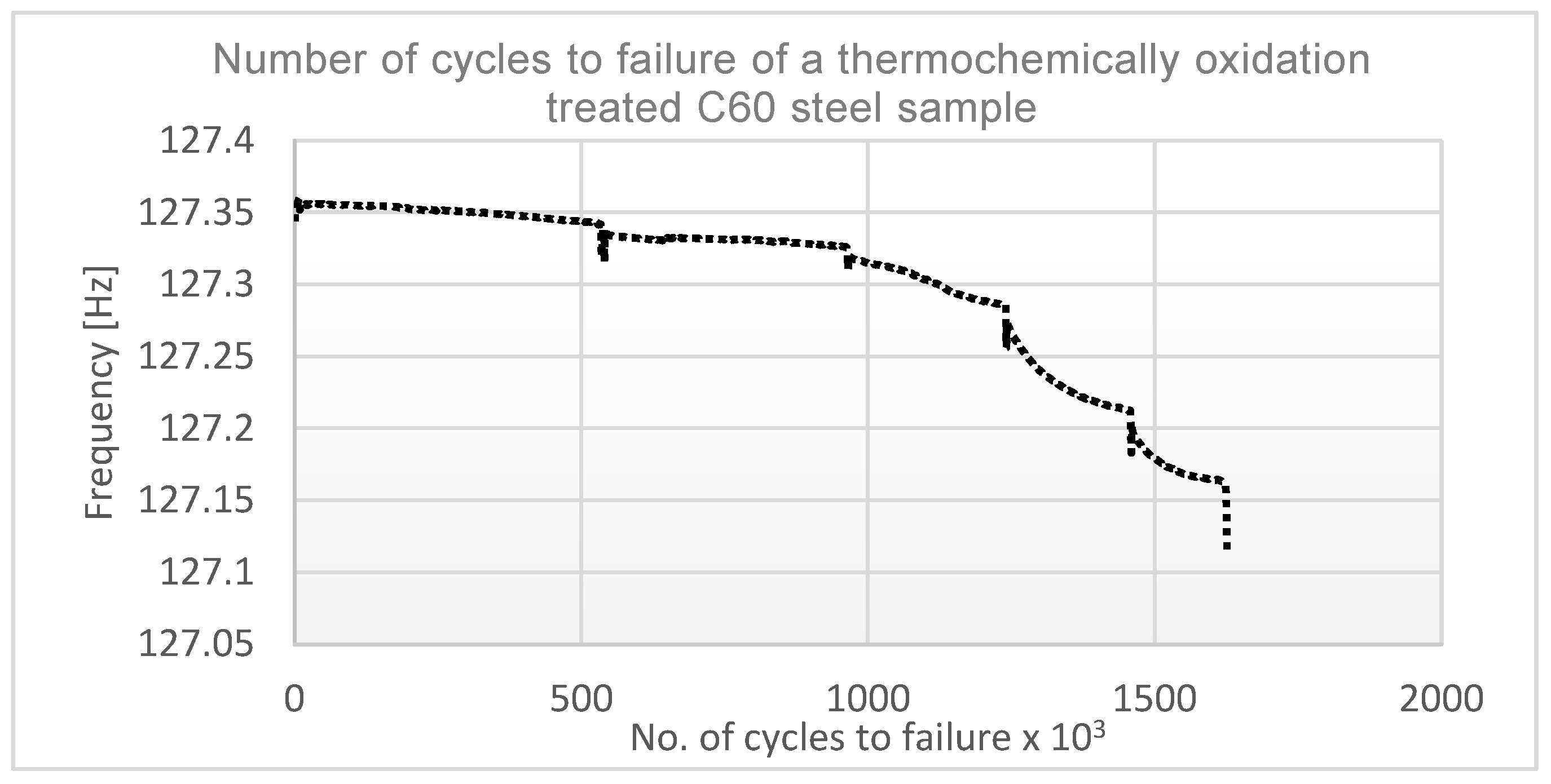
Figure 30.
Non-destructive analysis applied to oxidized Sample after fatigue testing: a) and b) liquid penetrant inspection and c) Overview of CT Examination d) Detail Volume Image-frontal surface of sample e) microcrack measurement in the frontal surface area, f) Detail Volume Image- radius area g) microcrack measurement in radius area.
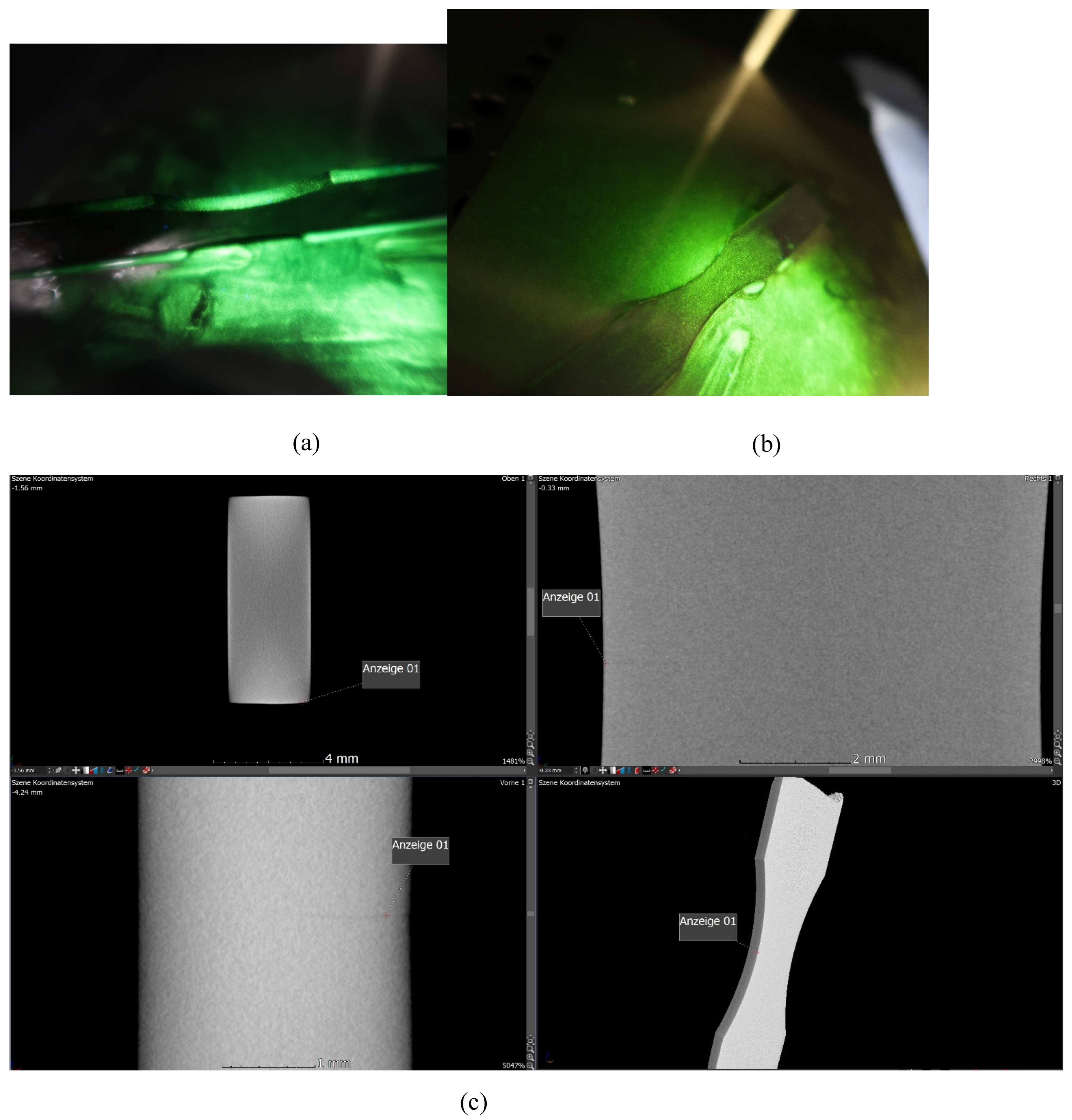
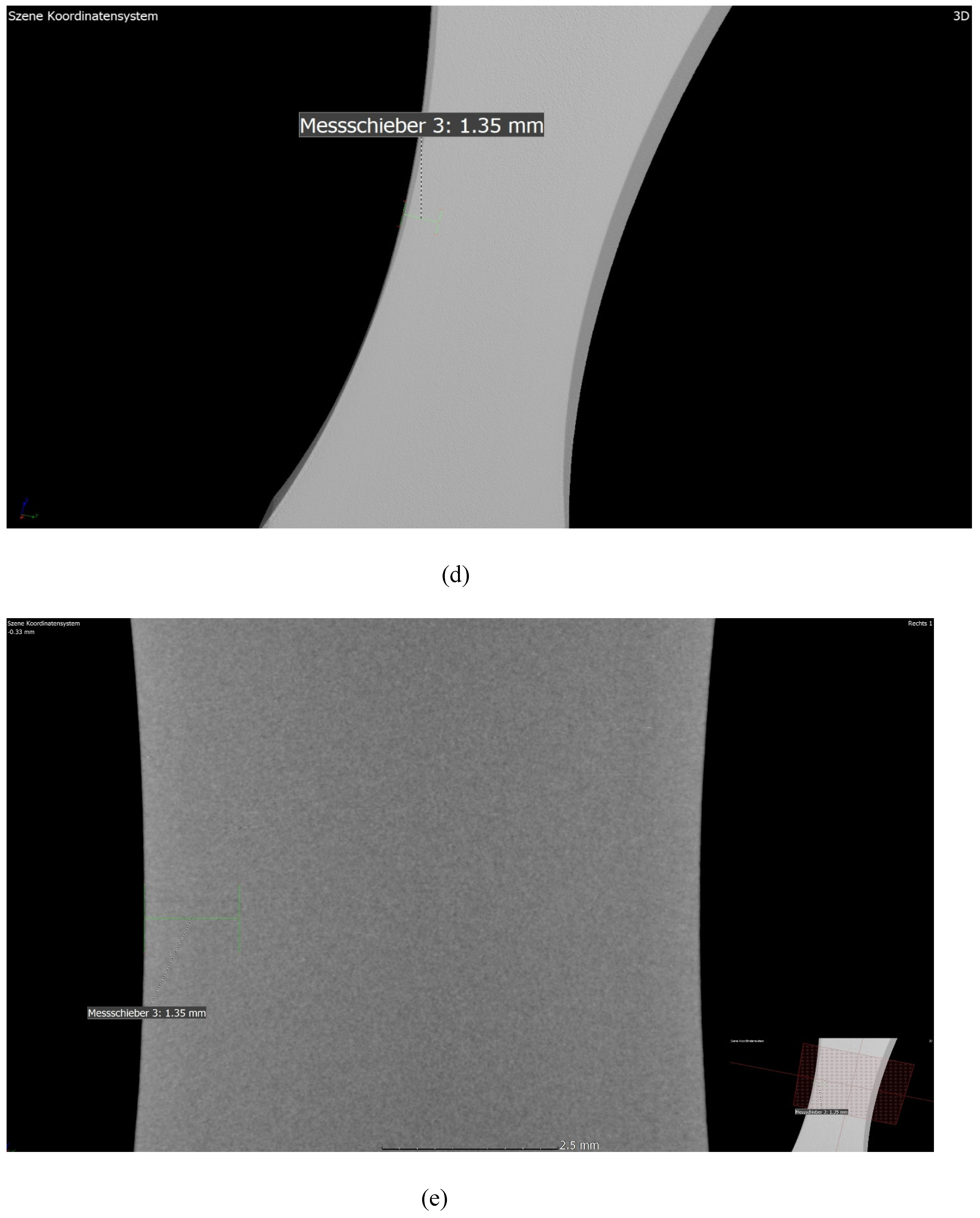
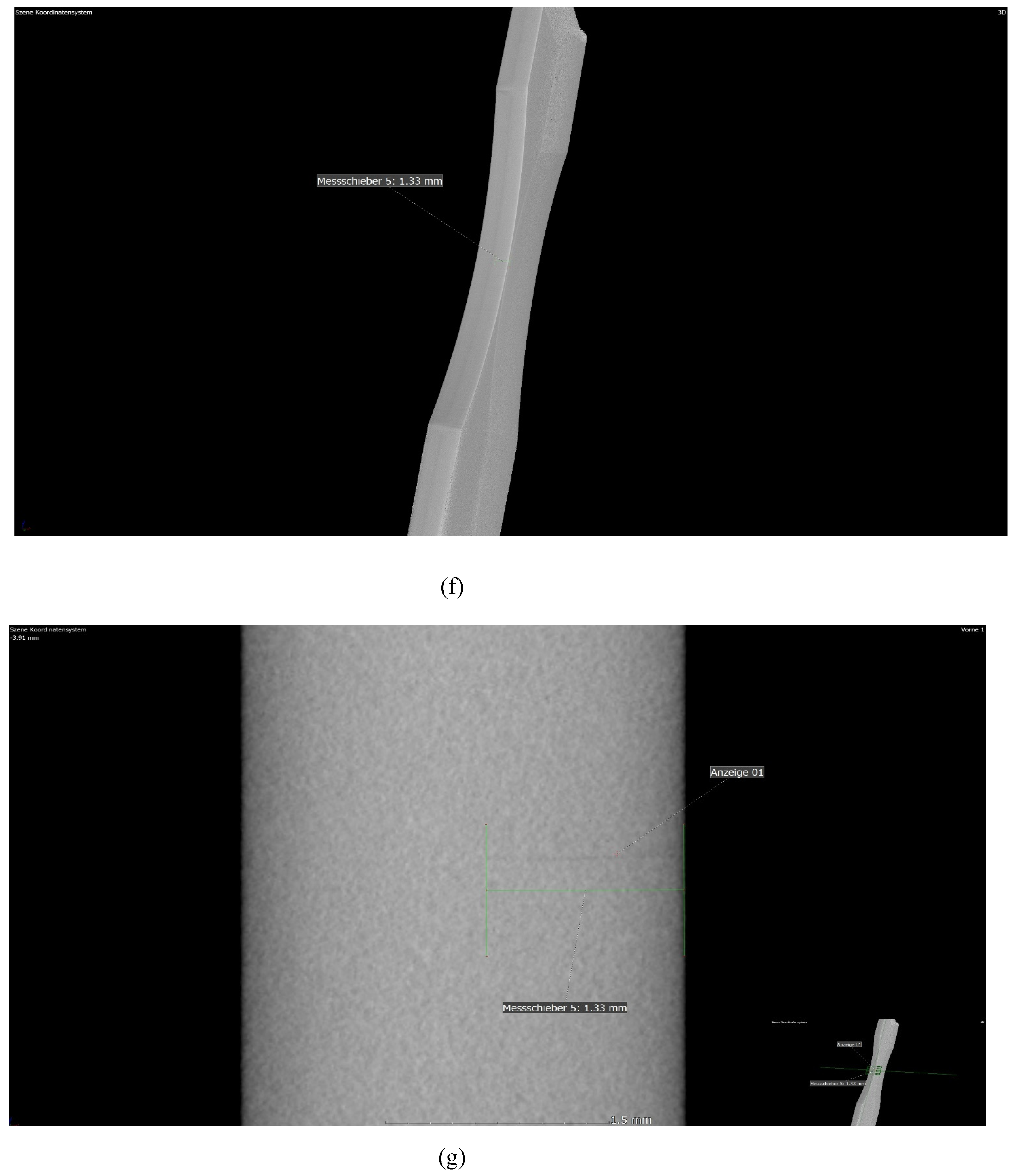
Table 1.
The planning of the experiment.
| Nr. crt | Stage | Targeted Results | Type of Testing | Place of Measurement |
|---|---|---|---|---|
| 1. | procurement of materials for experiments | 110x14x3 mm | Fa. Zelos Zerspanung Inh. Simon Oreskovic e. K.- Bessenbach, Germany |
|
| 2. | Check the chemical composition of material |
Composition of the material | Optical Emission Spectrometer | Fa. Liebherr Deggendorf |
| 3. | Identification of specimens |
Laser marking | Laser | Fa. Liebherr Deggendorf |
| 4. | thermochemical treatment-Oxidieren |
Gas oxidieren | Gas furnace | Fa. Härterei Reese Brackenheim |
| 5. | Analysis of Hardness and Microhardness | Obtained results |
Micro Hardness tester | Fa. Liebherr Deggendorf |
| 6. | Metallography Analyses |
Determination of microstructure | Stereo- and Light-microscopy | Fa. Liebherr Deggendorf |
| 7. | Fatigue testing | Number of cycles to fracture | Rumul MIKROTRON resonant testing machine for fatigue tests up to 20 kN | Fa. Liebherr Deggendorf |
| 8. | Non-destructive testing of specimens | Crack identification with magnetic powder | NDT-MT-Testing [magnetic particle testing) | Fa. Liebherr Deggendorf |
| Crack length measurement by computer tomography | CT (Computer tomography) | Technische Hochschule Deggendorf | ||
| 9. | The characterization of the oxide layer | analyzing the composition and thickness of the oxide layer formed on a material’s surface | GDOES (Glow Discharge Optical Emission Spectroscopy) | TAZ GmbH |
Table 2.
Chemical composition of C60 [1.0601] material purchased in thermally treated condition by hardening and tempering.
Table 2.
Chemical composition of C60 [1.0601] material purchased in thermally treated condition by hardening and tempering.
| Alloy Composition (at.%) | C | Si | Mn | P | S | Cr | Mo | Ni | Cr + Mo + Ni |
| DIN EN 10083-2 | 0,57-0,65 | max. 0,4 |
0,60-0,90 | max. 0,045 |
max. 0,045 |
max. 0,40 |
max. 0,10 |
max. 0,40 |
max. 0,63 |
| Analyse sample | 0,64 | 0,22 | 0,61 | 0,001 | 0,004 | 0,22 | 0,006 | 0,022 | 0,248 |
Table 3.
Hardness measurements on samples as delivered.
| Number of measurements | Hardness of sample surface | Mechanical strength | Hardness of the core surface | Mechanical strength |
|---|---|---|---|---|
| 1 | 416 HBW | 1317 MPa | 423 HV 30 | 1320 MPa |
| 2 | 414 HBW | 1310 MPa | 424 HV 30 | 1323 MPa |
| 3 | 414 HBW | 1310 MPa | 424 HV 30 | 1323 MPa |
Table 4.
The oxidation process Parameters.
| Section Nr. | 000 | 001 | 002 | 003 | 004 | 005 | 006 | 007 | 008 | 009 | 010 |
| Process |
Start | Heating without Gas | Vacuum | Heating with Gas | Heating with Gas | post- oxidation |
Heating with Gas |
post- oxidation |
Heating with Gas | post- oxidation |
Kühlen |
| Time | - | 000:01:00 | 000:01:00 | 001:30:00 | 000:30:00 | 000:45:00 | 000:15:00 | 000:45:00 | 000:30:00 | 000:45:00 | 000:01:00 |
| Temp. retort °C |
20 | 290 | 290 | 540 | 540 | 530 | 520 | 510 | 515 | 490 | 70 |
| Deltband °C | 0 | 10 | - | 10 | 5 | 5 | 5 | 5 | 5 | 5 | 5 |
| Drehzal U/min | 0 | 1470 | 1470 | 1470 | 1450 | 1470 | 1470 | 1470 | 1470 | 1470 | 1470 |
| H2O Menge l/h | - | - | - | - | - | 3,70 | - | 3,70 | - | 3,70 | - |
Table 5.
Hardness measurements on samples thermochemically treated by oxidation.
| Number of measurements |
Hardness of sample surface |
Mechanical strength | Microhardness of sample surface |
Mechanical strength | Hardness of the core surface | Mechanical strength |
|---|---|---|---|---|---|---|
| 1 | 330 HBW | 1048 MPa | 362 HV 0,05 | 1134 MPa | 293 HV 30 | 918 MPa |
| 2 | 327 HBW | 1039 MPa | 372 HV 0,05 | 1165 MPa | 293 HV 30 | 918 MPa |
| 3 | 332 HBW | 1054 MPa | 357 HV 0,05 | 1119 MPa | 295 HV 30 | 924 MPa |
Table 8.
The distribution of the number of cycles for the 13 tested samples.
| Probe 01 | 174600 |
x̄=205700 [samples tested to failure] |
| Probe 02 | 202800 | |
| Probe 03 | 239700 | |
| Probe 04 | 20000 |
Samples tested for fatigue at a predetermined number of cycles |
| Probe 05 | 40000 | |
| Probe 06 | 60000 | |
| Probe 07 | 80000 | |
| Probe 08 | 100000 | |
| Probe 09 | 120000 | |
| Probe 10 | 140000 | |
| Probe 11 | 160000 | |
| Probe 12 | 180000 | |
| Probe 13 | 200000 |
Table 12.
Fatigue to failure test results for oxidized samples.
| No. of sample | No. of cycles | Initial frequency [Hz] | Decrease in frequency [Hz] | Final frequency [Hz] |
|---|---|---|---|---|
| 01 | 1630529 | 127.352 | 127.330 | 105.208 |
| 02 | 1627490 | 127.350 | 127.342 | 105.192 |
| 03 | 1628025 | 127.368 | 127.340 | 105.189 |
| x̄=1628681 | x̄=127.35 | x̄=127.33 | x̄=105,19 |
Disclaimer/Publisher’s Note: The statements, opinions and data contained in all publications are solely those of the individual author(s) and contributor(s) and not of MDPI and/or the editor(s). MDPI and/or the editor(s) disclaim responsibility for any injury to people or property resulting from any ideas, methods, instructions or products referred to in the content. |
© 2025 by the authors. Licensee MDPI, Basel, Switzerland. This article is an open access article distributed under the terms and conditions of the Creative Commons Attribution (CC BY) license (http://creativecommons.org/licenses/by/4.0/).
Copyright: This open access article is published under a Creative Commons CC BY 4.0 license, which permit the free download, distribution, and reuse, provided that the author and preprint are cited in any reuse.


