Submitted:
16 April 2025
Posted:
17 April 2025
You are already at the latest version
Preprints on COVID-19 and SARS-CoV-2
Abstract
COVID-19’s effects on mortality are hard to quantify. Issues with attribution can cause problems with resulting conclusions. Analyzing excess mortality addresses this concern and allows for the analysis of broader effects of the pandemic. We propose separate ARIMA models to analyze excess mortality for several countries. For the model of joint excess mortality, we suggest vine copulas with Bayesian pair copula selection. The present study examines weekly mortality data from 2019-2022 in the USA, Canada, France, Germany, Norway, and Sweden. Proposed ARIMA models have low lags and no residual autocorrelation. Only Norway’s residuals exhibited normality, while remaining suggest skewed Student-t distributions as a plausible fit. A vine copula model was then developed to model the association between the ARIMA residuals for different countries, with the countries farther apart geographically exhibiting weak or no association. The validity of fitted distributions and resulting vine copula was checked using 2023 data. Goodness of fit tests suggest that the fitted distributions were suitable, except for the USA, and that the vine copula used was also valid. We conclude that the time series models of COVID-19 excess mortality are viable. Overall, the suggested methodology seems suitable for creating joint forecasts of pandemic mortality for several countries or geographical regions.
Keywords:
ARIMA
; pair copula
; vine copula
; Bayesian analysis
1. Introduction
The COVID-19 pandemic began in late 2019, and quickly manifested itself as a massive increase in global mortality. However, there were problems related to attribution and causation. As such, when it comes to analyzing or modeling COVID-19 mortality data, there are two approaches. The first is to specifically use COVID-19-attributed mortality. This has the benefit of a clear causal structure, where patterns in the data can be more easily connected to the spread of the pandemic [19]. However, there are notable problems with respect to proper attribution. Deaths related to COVID-19 are not attributed to the disease absent a positive COVID-19 test, which is not always possible in locations unable to test [26]. This is to say nothing of other infrastructure issues or potentially missing deaths not directly caused by COVID-19, but instead by complications from an existing condition or a response to the pandemic [26,28]. However, using mortality data directly attributed to COVID-19 comes with the massive benefit of no ambiguity.
The second approach is to analyze overall mortality, usually via the concept of excess mortality. This is defined as the normalized difference between an expected (historical) death count and aggregate deaths [9]. Although there is some ambiguity in calculating the expected number of deaths for a particular location, this approach has the benefit of capturing systemic effects the pandemic might have had [21,28]. For example, it allows data to include the effects of increased mortality in those with existing conditions of contracting COVID-19 [21], or possible increases in suicides [19]. However, the data will also reflect a decrease in vehicle-related deaths due to lock-downs [26]. This approach captures the net effect and accurately reflects the total effect of the pandemic. However, it also carries the possible risk of masking the magnitude of the positive effect on mortality.
Regardless, multiple approaches are used to model the resulting data. The Center for Disease Control (CDC) has suggested ensemble models [17], in [16], and in [26]. [21] and [4] used generalized additive models to relate different demographic or location data with mortality. ARIMA models are used frequently. For listed examples, see [19] and [26]. Copula models are also used to determine the relationships between mortality and other time series data, such as the correlation of interstate trends [18], or by combining mortality data with temperature [3]. Here we follow the method laid out by [19], in which ARIMA models are developed for individual locations, and the model residuals are then related to each other via copula analysis. This allows for seasonality and intra-country effects to be accounted for before addressing cross-correlation between countries. This also allows for the non-normal residuals, which while technically a violation of ARIMA assumptions, allows for the interpretation of fat-tailed residual distributions as an indication of a more complicated dependence structure.
The present paper has an objective of analyzing excess mortality time series for different countries during the period of T weeks and modeling the dependence patterns in the vector through the ARIMA residuals .
Mortality statistics are particularly difficult to compare across countries for several reasons. First and foremost, different countries have different standards for recording deaths. For example, England records only the date a death is “registered,” while the United States records mortality statistics using the date of a death [4,22]. This means comparisons involving countries who do not record the date of a death are difficult, as actual mortality experience will not be reflected in the data. While a close reconstruction of weekly data is possible (see [21]), it still leaves open the potential problem of a death being registered several weeks after it occurs, making assigning the week it occurred impossible. Second, countries differ in how they define a “week” and how many there are in the calendar year. For example, the European countries in this study (France, Germany, Norway, Sweden) record their weekly mortality data as the sum of deaths occurring from Monday-Sunday, while the United States and Canada record theirs as the sum of deaths from Sunday to Saturday [22]. This makes interpretations of resulting models somewhat weaker, but absent massive spikes for one day only, it should not affect overall trends.
2. ARIMA
Box-Jenkins models, more commonly known as ARIMA models, stand for autoregressive integrated moving average models of a time series. They have lag (order) for the single variable time series ,
integrated with the moving average model with lag ,
which is applied to the differences of with order ,
where allows the specification of non-stationary models as defined as ARIMA . Here corresponds to the the stationary model ARIMA also known as ARMA .
ARIMA model selection requires the estimation both of and the subsequent parameters in the regression models. This is usually done via Bayesian or maximum likelihood methods. This yields fitted values of for and residuals .
Unit root tests or other stationarity tests can be used to determine the differencing order d, which can be further informed by the behavior of the ACF or PACF of the time series data. Afterwards, the lag order parameters can be determined via information criterion, such as the Akaike and Bayesian (Schwarz) information criteria. Note that in the case of either the AIC or BIC, there is a penalty term for the number of parameters, leading to more parsimonious models if the information criteria are used for model selection. Note also that changing the value of d does not change the number of parameters to be estimated.
3. Distribution Analysis of ARIMA Residuals
In general, ARIMA methods are efficient in the assumption of normality of the residuals . However, in many applications, especially survival analysis and finance, one has to deal with asymmetric and fat-tailed residual distributions failing the normality assumption. Therefore, a Skewed-t distribution model, such as the one put forward by [12] may be suitable to the describe the distribution of residuals. The PDF defined therein is as follows.
Regardless, fitted distributions should be compared to residual data to ensure accuracy. A common test is the Kolmogorov-Smirnov test, which compares empirical CDFs between two different samples of data and/or distributions. Once a distribution has been chosen, the residuals can be appropriately modeled as random variables.
In the case of several dependent time series , k separate models can be developed for the marginal distributions of , which will help further construction of the joint distribution of , which is the ultimate goal.
4. Copula Analysis
Copula analysis is commonly used to model non-linear statistical dependence between two or more random variables. Copulas are special functions that can describe dependence of random variables as an association between their marginal distributions. In the present paper, copula analysis is applied to model the joint distribution of ARIMA residuals using the marginal distributions obtained in the previous section.
Let be random variables, with CDFs and . Then their joint distribution of can be represented using a copula function , where r is some set of parameters measuring the strength of dependence between the two variables.
Sklar’s theorem states that any copula function of u and v is a valid CDF of , and that any joint distribution function can be represented as a copula function of the marginals. Therein lies the advantage of copulas, because the copula analysis framework allows for the separation of modeling the marginals from modeling their association.
There are many different types of copulas to model association. For an in-depth list and definitions, see [6]. Most popular copulas used in practice are either Archimedean copulas or elliptical copulas. The former are easier to estimate parameters for, while the latter are easier to extend to higher dimensionality, e.g., more marginals.
Several techniques exist for estimating copula parameters. One way of doing it is to use non-parametric measures of sample correlation, namely Kendall’s concordance or Spearman’s , as many two-parameter copulas and all single-parameter copulas can have their parameters expressed as a measure of correlation, allowing for a direct substitution [6]. This relationship also allows for Bayesian analysis based on sample correlation. This is discussed later. Another approach is to use maximum likelihood estimation, though this could carry computational issues relating to a lack of closed form estimators [6,13]. For other parametric approaches, see [6] and [20]. For a non-parametric method, see [20].
Methods used to determine copula selection will be discussed later.
5. Vine Copulas
A single copula may not be an adequate model in higher dimensions. In these cases, a vine copula or pair-copula structure may be preferable. Vine copulas work by establishing several trees of time-series variables, then relating individual edges using pair copulas. Using Sklar’s theorem, the joint distribution of the data can be represented using a copula function of the marginals.
From here, differentiation yields the following.
For two variables, this simplifies to
which using basic properties of probability can be rewritten as
Extending this to three variables yields
which in turn can be extended to much higher dimensions. For that and more details, see [1] and [5]. Regardless, this implies that any joint distribution can be represented as the product of marginals, any existing pair copulas of the component vectors, and any existing conditional pair copulas. In the case of independence between two variables,
sunstantially simplifying the resulting structure.
Note that when working with vine copulas, the structure of the model must be specified before pair copulas can be estimated. In other words, which variables are independent of each other, which variables are conditioned on the others, and in what order, has to be determined first. For a detailed explanation why this approach is advantageous, see [1] and [5]. To estimate a structure, one can use the method put forth by [10]. First, the unconditional copulas are selected from the list of all possible structures, which can be exhaustive, based on which structure minimizes the reference statistic, such as AIC or BIC. Then pair copulas and their parameters are estimated for each non-independent pair. Then a variable is selected to be conditioned on, and the process repeats until all variables are exhausted.
6. Pair Copula Selection
Once a model structure has been specified, there are several ways to select the optimal copula(s). Most involve specifying a potential set of hyperparameters defined for each copula family, and then comparing them. This can be done using the AIC [6,8,20], BIC [6], or other information criterion. Various goodness-of-fit tests also can be used for this purpose, allowing for their statistics to be compared to select a copula [14]. However, as [14] points out, this approach compares single copula models with given parameter values chosen from each parametric family, instead of selecting a copula based on multiple possible parameter values.
A solution to this is to select copulas using Bayesian inference. [27] describes the following method, which was suggested in [14] and also used in [24]. First, let be the hypotheses that the data comes from one of M copula families, and for each pair test . These hypotheses can be assumed to be mutually exclusive and exhaustive. Then, let be Kendall’s concordance. If all considered copulas can be written as a function of , the posterior probabilities of hypotheses given data may be rewritten as
where is the prior probability of . [27] show that this method still yields good results even for vague or non-informative priors on . Since and in case of positive dependence , uniform Beta will be a suitable choice for . Since the posterior probabilities are only to be used for selection purposes, does not need to be calculated. With the discrete uniform prior on the hypothesis choice, it suffices to calculate the weights with denoting respective copula p.d.f.:
or, using a Monte-Carlo approach and drawing N samples from the uniform prior, evaluate
and then the posteriors
for each pair .
7. Results
As stated above, data from certain countries during the pandemic may be unreliable, due to lack of infrastructure, intentional misreporting, missing data, etc. This study chose to focus on mortality data from the United States, Canada, France, Germany, Norway, and Sweden because of the easy availability of their mostly reliable data recorded in a similar time frame. For each country in this study, the following sources were used. The United States’ mortality data were obtained through the Center Disease Control’s (CDC) website. Canada’s data were obtained through Statistics Canada, and they adhere to the same standards as the US [15]. The European countries’ data were obtained entirely through EuroStat, the official statistics body for the European Union [11]. The six countries in this study record the number of weeks in the year as the same, which is 52 (or 53) full 7-day weeks [15]. This fixes the problem of weeks being out of alignment in which year they occur,as the data presented differs by one day only between the North American and European time series. Mortality data from 2014-2018 was used to used to make 5-year weekly averages. With 2014 being the only year with 53 weeks, this means week 53’s mortality average for each country is simply the last week of 2014. For pandemic data, the first week of 2019 through the 52nd week of 2022 was used. To compute excess mortality, the difference between each country’s pandemic data and historical data was recorded as a percentage of the historical data in a time series.
7.1. ARIMA
To begin, each time series was tested for stationarity using the Augmented Dickey-Fuller test and KPSS tests through the tseries R package. The p-values are summarized in Table 1.
The mixed results do not give a clear indication as to whether the time series are stationary or not.
From here, partial autocorrelation functions for each time series were analyzed. The United States showed no significant correlation after a lag of 3. France, Germany, and Sweden showed no significant correlation for a lag of 2, but did have significant correlation for higher order lags. Canada and Norway showed no significant correlation after a lag of 2. After this, ARIMA analysis was performed using the ARIMA function from the R package stats to generate potential models. Final models were selected first by those with a nonzero amount of statistically significant coefficients, and then by BIC. The models were built according to the structure of the following equation:
where is the error terms, and is the intercept. The results are summarized in the following table.
After models were selected, each model’s residuals were subject to a Box-Ljung test using the stats R package. The results are summarized in Table 3.
7.1.1. ARIMA Residual Analysis
After this, the Shapiro-Wilk test was performed on each model’s residuals to determine their normality.

Table 4.
Shapiro-Wilk Tests.
| Country | P-Values |
|---|---|
| USA | |
| CAN | |
| FRA | |
| GER | |
| NOR | |
| SWE |
This suggests only the residuals for Norway’s model were normal. Fitting the distribution using fitdistr function from the R package MASS yielded a normal distribution with and . To fit a distribution to the others, the skewed t-distribution as defined in [12] was used. The results of the fitted distributions are summarized in Table 5.
Results were verified using the Kolmogorov-Smirnov test, which is summarized in the following table. D is the test statistic. For the test, due to errors caused by the ks.test function used, which was not compatible with the distribution functions fitted, fitted distributions had samples randomly drawn from them to be compared, with a sample size of .
Table 6.
Kolmogorov-Smirnov test statistics and P-values.
| Country | D | P-Value |
|---|---|---|
| USA | ||
| CAN | ||
| FRA | ||
| GER | ||
| SWE |
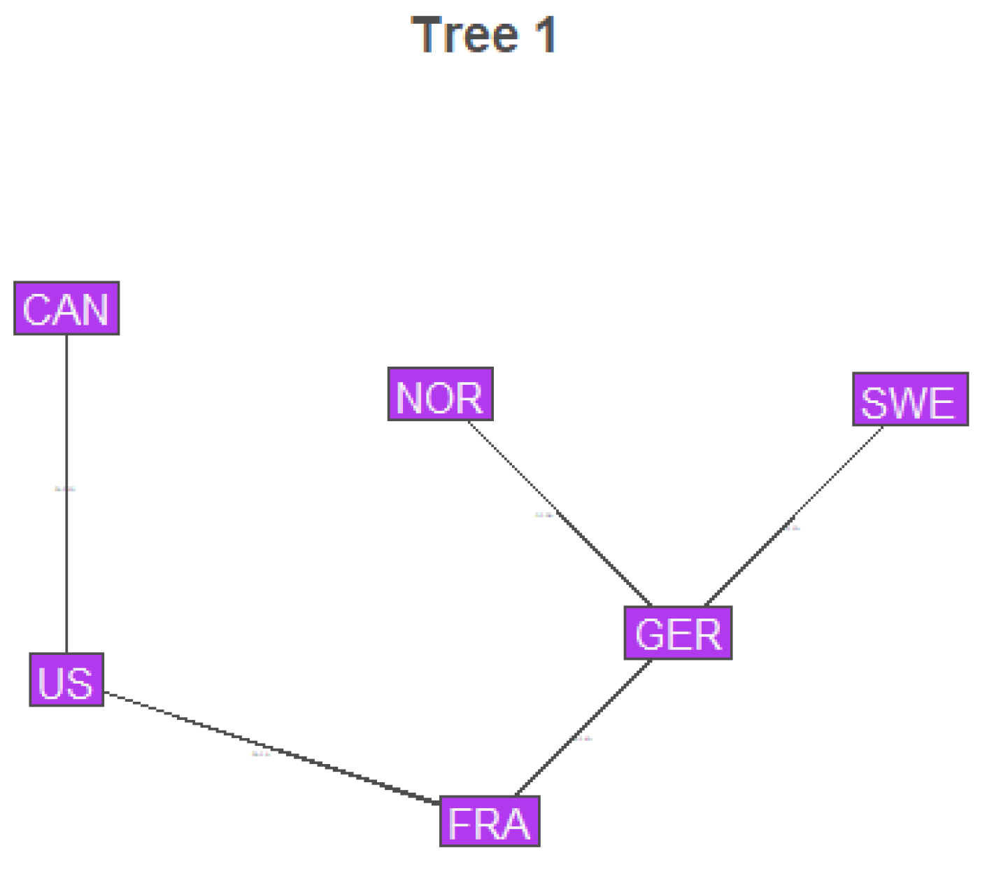
7.2. Vine Structure Selection
Structure of the copula model was determined using the RVineStructureSelect function from the VineCopula R package. Later procedures determined all copulas after the first tree to be independence copulas, so only the structure of the first tree will be shown.
Figure 1.
Vine Structure
7.3. Copula Selection
Pair copula selection was performed using the Bayesian method outlined in [24]. First the assumption was made that each copula would fall into one of 4 hypothesized copula families.
7.3.1. Hypothesis 1 (H1) Clayton’s Copula, C
7.3.2. Hypothesis 2 (H2) Gumbel-Hougaard’s Copula, G
7.3.3. Hypothesis 3 (H3) Dual (Survival) Clayton’s Copula, SC
7.3.4. Hypothesis 4 (H4) Dual Gumbel-Hougaard’s Copula, SG
Next, optimal were selected using MLE, resulting in the following structure.
Table 7.
Posterior Probabilities for Hypothesized Pair-Copula Families
| Countries | US/CAN | US/FRA | FRA/GER | GER/NOR | GER/SWE |
|---|---|---|---|---|---|
| H1 (C) | 0 | ||||
| H2 (G) | |||||
| H3 (SC) | 0 | 0 | |||
| H4 (SG) |
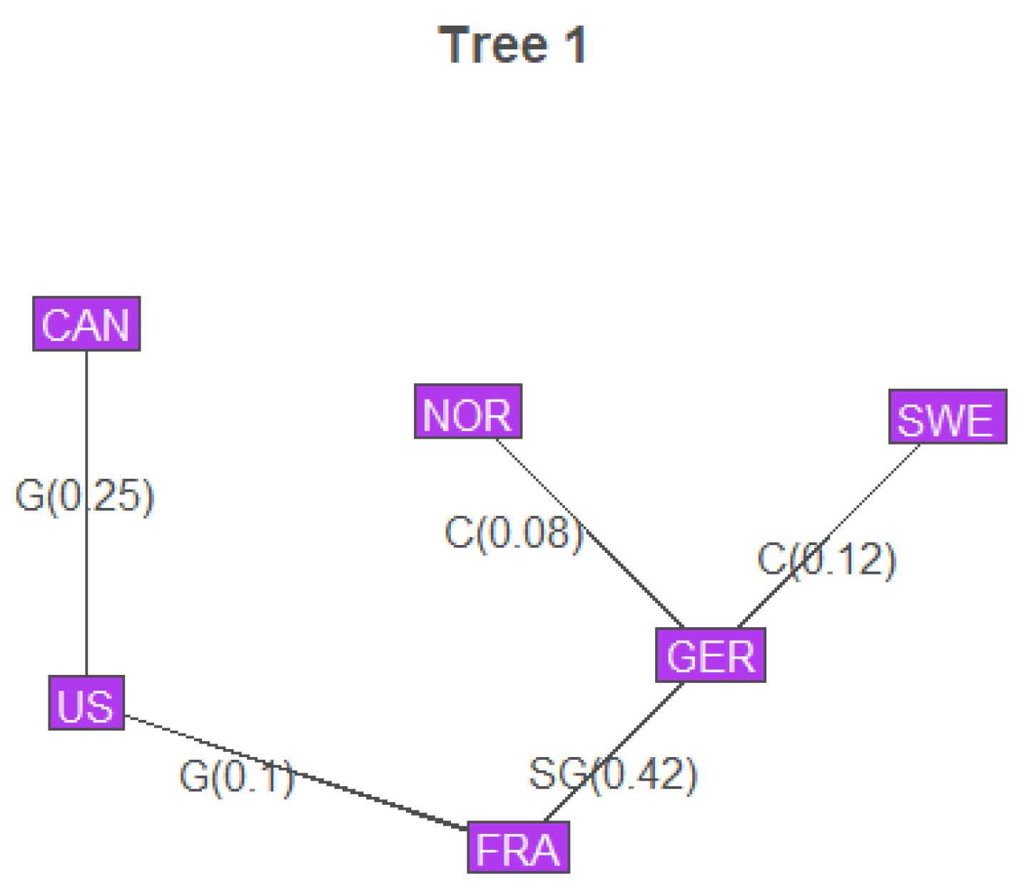
Figure 2.
Vine Structure with the Pair Copulas and and
8. Validation
To validate results, mortality data from 2023 was used. While Eurostat maintained weekly death counts throughout 2023, the CDC only maintained weekly counts for 36 weeks, and Statistics Canada only maintained weekly counts for 33 weeks. This does not impact the analysis of ARIMA models, since it is done country-by-country, meaning all available data can be used. To validate ARIMA models and earlier marginal analysis, the existing ARIMA models were applied to generate residuals, then those residuals were compared to previously fitted distributions using a Kolmogorov-Smirnov test, using the same distribution samples as earlier for the skew-t distributions. For Norway, a new sample was generated. The results are summarized in the following table.
Table 8.
Kolmogorov-Smirnov test statistics and P-values.
| Country | D | P-Value |
|---|---|---|
| USA | ||
| CAN | ||
| FRA | ||
| GER | ||
| SWE | ||
| NOR |
This suggests that the marginal distributions of the residuals fitted in the Results section are accurate for Canada, France, Germany, Sweden, and Norway, and potentially not accurate for the USA. This makes some sense, as the Pandemic was seen as winding down in the US by the time the CDC stopped updating its weekly death count. As such, models developed from Pandemic mortality experience would probably not be as accurate.
Afterwards, to validate the copula model proposed in the Results section, the data length had to be adjusted for each country’s residuals. To accomplish this, each data set was limited to the first 33 weeks. Then, the residuals were transformed to a uniform sample. Finally, this sample was compared using the VineCopula R package’s RVineGofTest function to the existing copula structure using the Kolmogorov-Smirnov test (evaluated asymptotically), and the Cramer-von-Mises Test (evaluated with 200 bootstrap steps). The results are summarized in the follow table. For more details on how these tests are implemented in the package for vine copulas, see [23].
Table 9.
KS and CvM test P-values for Vine Copula Model
| Test | P-Value |
|---|---|
| KS | |
| CvM |
This suggests that the dependency model put forth by the vine copula found in the Results section describes the connections between the countries’ mortality experience well, even when the mortality experience differs from what is expected.
9. Conclusions
Time-series models of COVID-19 excess mortality are viable. ARIMA models have low lags and no residual auto correlation, but model residuals tend to be non-normal, being skewed with fat tails. In addition, there appears to be cross-correlation between countries not otherwise captured by ARIMA models. This can be modeled using vine copula structures, with pair copulas being appropriately selected via Bayesian analysis of different hypothesized families. The end result also demonstrates a geographic component in determining the association between different countries’ residuals. Neighboring countries tend to have higher correlations with each other versus countries separated by an ocean. However, this is not always the case, as Norway and Sweden’s model residuals appeared to be independent of each other, and were more closely related with Germany’s residuals. Model validation showed that real-world experience towards the end of the pandemic differed somewhat from model predictions, possibly due to decreases in mortality. However, the dependence structure held, suggesting that the conclusions derived from the vine copula model were accurate. Overall, this template seems suitable for creating joint forecasts of pandemic mortality for several countries.
Author Contributions
Conceptualization, A.S.; methdology, J.A. and A.S.; software, J.A.; validation, J.A.; formal analysis, A.S. and J.A.; investigation, A.S. and J.A.; resources, J.A. and A.S.; data curation, J.A.; writing—original draft preparation, A.S. and J.A.; writing—review and editing, J.A. and A.S.; visualization, J.A. and A.S.; supervision, A.S.; projection administration, A.S.; funding acquisition, A.S. All Authors have read and agreed to the published version of the manuscript.
Funding
This research received no external funding.
Institutional Review Board Statement
Not applicable.
Informed Consent Statement
Not applicable.
Data Availability Statement
The original contributions presented in this study are included in the article/supplementary material. Further inquiries can be directed to the corresponding author(s).
Acknowledgments
We would like to acknowledge the support of CAM (Center for Applied Mathe-matics) at the University of St. Thomas and assistance of Rebecca Twite (UST) in modeling and simulation during Summer 2023.
Conflicts of Interest
The authors declare no conflicts of interest.
Abbreviations
The following abbreviations are used in this manuscript:
| AIC | Akaike Information Criterion |
| ARIMA | Auto-Regressive Integrated Moving Average |
| BIC | Bayesian Information Criterion |
| CDC | Center For Disease Control |
| CDF | Cumulative Distribution Function |
| CvM | Craner-von Mieses (test) |
| KPSS | Kwiatkowski–Phillips–Schmidt–Shin (test) |
| KS | Kolmogorov-Smirnov (test) |
| Probability Distribution Function |
Appendix A
Data and relevant code are available at this link.
References
- Aas, K., Czado, C., Frigessi A., and Bakken H. 2009. Pair-Copula constructions of multiple dependence. Insurance: Mathematics and Economics 44: 182–198.
- Ahamad MG, Tanin F, Talukder B, Ahmed MU. 2020. Officially Confirmed COVID-19 and Unreported COVID-19-Like Illness Death Counts: An Assessment of Reporting Discrepancy in Bangladesh. Am J Trop Med Hyg. 104(2):546-548.
- Alanazi, Fahad. 2021. The spread of COVID-19 at Hot-Temperature Places with Different Curfew Situations Using Copula Models. Paper presented at 1st International Conference on Artificial Intelligence and Data Analytics (CAIDA), Riyadh, Saudi Arabia, April 6–7.
- Basellini U., Alburez-Gutierrez, D., Del Fava, E., Perrotta,D., Bonetti M., Camarda, C.G., Zagheni, E. Linking excess mortality to mobility data during the first wave of COVID-19 in England and Wales. 2021. SSM - Population Health. 14.
- Bedford, T., and Cooke, R. M. 2001. Probability Density Decomposition for Conditionally Dependent Random Variables Modeled by Vines. Annals of Mathematics and Artificial Intelligence 32(1-4): 245-268.
- Brechmann, E. 2010. Truncated and simplified regular vines and their applications. Technische Universität München. Munich, Germany.
- Brechmann, E. C., Czado, C., and Aas, K. 2012. Truncated regular vines in high dimensions with application to financial data. Canadian Journal of Statistics 40(1): 68-85.
- Brechmann, E. C., and Schepsmeier, U. 2013. Modeling Dependence with C-and D-Vine Copulas: The R Package CDVine. Journal of Statistical Software 52(3): 1-27.
- Britt, Tom, Jack Nusbaum, Alexandra Savinkina, and Arkady Shemyakin. 2023. Short-term Forecast of U.S. COVID Mortality Using Excess Deaths and Vector Autoregression. Model Assisted Statistics and Applications 18: 13–31. https://doi.org/10.3233/mas-221392.
- Dissmann, J. F., Brechmann E. C., Czado C., and Kurowicka D. 2013. Selecting and estimating regular vine copulae and application to financial returns. Computational Statistics & Data Analysis 59(1): 52-69.
- Eurostat. Available online: https://ec.europa.eu/eurostat/data/database (accessed on 15 Feb 2025).
- Fernandez, C. and Steel, M.F.J. 1996. On Bayesian Modelling of Fat Tails and Skewness. Journal of the American Statistical Association 93(441): 359-371.
- Huang L, Shemyakin A. 2020. Empirical comparison of skewed t-copula models for insurance and financial data. Model Assisted Statistics and Applications 15(4):351-361.
- Huard D., Evin G., and Favre A.C. 2006. Bayesian copula selection. Computational Statisticss & Data Analysis 51(2): 809-822.
- Human Mortality Database. 2025. Short-Term Mortality Fluctuations Data Series Note.Available online: https://www.mortality.org/File/GetDocument/Public/STMF/DOC/STMFNote.pdf (accessed 15 Feb 2025).
- Imperial College COVID Response Team. 2022. Short-Term Forecasts of COVID-19 Deaths in Multiple Countries. May. Available online: https://mrc-ide.github.io/covid19-short-term-forecasts/ (accessed on 15 February 2025).
- Johansson, Michael A., Nicholas G. Reich, Evan L. Ray, Nutcha Wattanachit, Abdul Hannan Kanji, Katie House, Estee Y. Cramer, Johannes Bracher, Andrew Zheng, Teresa K. Yamana, and et al. 2020. Ensemble Forecasts of Coronavirus Disease 2019 (COVID-19) in the U.S. medRxiv.
- Kim, Jong-Min. 2022. Copula Dynamic Conditional Correlation and Functional Principal Component Analysis of COVID-19 Mortality in the United States. Axioms 11:619.
- Lei, X. and Shemyakin A. 2023. Copula Models of COVID-19 Mortality in Minnesota and Wisconsin. Risks 11: 193.
- Manner, Hans. 2007. Estimation and Model Selection of Copulas with an Application to Exchange Rates. Meteor Research Memorandum 56.
- Martinez-Folgar, K., Alburez-Gutierrez, D., Paniagua-Avila, A., Ramirez-Zea, M., and Bilal, U. 2021. Excess mortality during the COVID-19 pandemic in Guatemala. American Journal of Public Health 111(10):1839-1846.
- National Center for Health Statistics. Weekly Counts of Deaths by State and Select Causes, 2014-2019; 2020-2023. Available online: https://data.cdc.gov/d/3yf8-kanr and https://data.cdc.gov/d/muzy- jte6.
- Schepsmeier, U. 2015. Efficient information based goodness-of-fit tests for vine copula models with fixed margins. Journal of Multivariate Analysis 138, 34-52.
- Shemyakin, Arkady, and Alexander Kniazev. 2017. Introduction to Bayesian Estimation and Copula Models of Dependence. London: John Wiley and Sons, 345p, ISBN 978-1-118-95901-5.
- Statistics Canada. Table 13-10-0768-01 Provisional weekly death counts, by age group and sex. 2024. Available online:https://www150.statcan.gc.ca/n1/pub/71-607-x/71- 607- x2021028-eng.htm (accessed on 15 Feb 2025).
- Wang et al. Estimating excess mortality due to the COVID-19 pandemic: a systematic analysis of COVID-19-related mortality, 2020-21. Lancet 399(10334):1513-1536.
- Wifvat, K., Kumerow, J., and Shemyakin, A. 2020. Copula Model Selection for Vehicle Component Failures Based on Warranty Claims. Risks 8(2):56.
- Zińczuk A, Rorat M, Jurek T. 2023. COVID-19-related excess mortality - an overview of the current evidence. Arch Med Sadowej Kryminol 73(1):33-44.
Table 1.
Stationarity Test P-values.
| Country | ADF | KPSS |
|---|---|---|
| USA | ||
| CAN | ||
| FRA | ||
| GER | ||
| NOR | ||
| CAN |
Table 2.
ARIMA Coefficients and Standard Errors by Country
| Coef | USA | CAN | FRA | GER | NOR | SWE |
|---|---|---|---|---|---|---|
| - | - | |||||
| - | - | - | - |
Table 3.
Box-Ljung Tests.
| Country | P-Values |
|---|---|
| USA | |
| CAN | |
| FRA | |
| GER | |
| NOR | |
| SWE |
Table 5.
Skewed-t Fit Results
| Country | 1 | v | ||
|---|---|---|---|---|
| USA | 0 | |||
| CAN | 0 | |||
| FRA | 0 | |||
| GER | 0 | |||
| SWE | 0 |
1 was found to be both and have high standard error, as such as each mean was treated as zero.
Disclaimer/Publisher’s Note: The statements, opinions and data contained in all publications are solely those of the individual author(s) and contributor(s) and not of MDPI and/or the editor(s). MDPI and/or the editor(s) disclaim responsibility for any injury to people or property resulting from any ideas, methods, instructions or products referred to in the content. |
© 2025 by the authors. Licensee MDPI, Basel, Switzerland. This article is an open access article distributed under the terms and conditions of the Creative Commons Attribution (CC BY) license (http://creativecommons.org/licenses/by/4.0/).
Copyright: This open access article is published under a Creative Commons CC BY 4.0 license, which permit the free download, distribution, and reuse, provided that the author and preprint are cited in any reuse.


