
Submitted:
15 April 2025
Posted:
21 April 2025
You are already at the latest version
Abstract
In the ISO 2859 and ISO 3951 series, the acceptance sampling plans have relatively large sample size values. For this reason, it is interesting to develop an approach to acceptance sampling based on Bayesian statistics. In the present paper, this focus is on Bayesian plans developed from the perspective of utility, understood as benefits minus costs. This focus on utility rather than on risk allows a completely different approach to acceptance sampling plans to be developed. The utility is defined via three simple parameters and it is shown how sample size and acceptance number can be calculated by maximizing utility. The calculation is further refined via a hierarchical model which tests the prior distribution against the empirical data. Finally, tables of standard plans are provided for the practitionner.
Keywords:
acceptance sampling plan
; Bayesian statistics
; utility
; costs
; regret
; hierarchical Bayesian model
; standard plans
1. Introduction: Risk Versus Utility
The acceptance sampling plans described in the ISO 2859 and ISO 3951 series 1 have several drawbacks. In particular, for many plans, the sample size values are quite large. Moreover, the producer’s and consumer’s risks may be greater than what may be considered acceptable1. For example, the “main diagonal” plans in ISO 2859-12 (normal inspection) result in a producer’s risk of circa 12% (calculated via the binomial distribution). In developing Bayesian approaches for the design of acceptance sampling plans, the aim is thus twofold: reduce sample size values and improve risk levels. Both aspects are addressed in the risk-based approach described in Uhlig et al. (2024) 9. In particular, a framework was introduced in which the Bayesian risks3 and the “classical” risks from the ISO standards can be considered complementary. In the present paper, Bayesian plans are developed from an entirely different perspective. The focus is now on the utility, which can be broadly understood as benefits minus damages and costs.
Insofar as risks are understood as the probability that costs are incurred, it can be stated that a utility-based approach (encompassing both costs and benefits) is broader than a risk-based approach. Indeed, a calculus based solely on risks is often unnecessarily narrow. Taking the logic of risks to its extreme, the best course of action is often undertaking nothing at all, thus avoiding risk altogether. In other words, risk aversion, taken as the basis for decision making, will often lead to inaction. Indeed, a focus on risks often reflects the knee-jerk resort to a certain type of test in traditional statistics, where statistically significant results4 can be interpreted as risks for one or the other party. However, the relevant question is not whether a given (and somewhat arbitrary) level of risk is exceeded. In assessing an acceptance sampling plan, instead of considering only the level of risk, the central question should be: can rational risk-taking be distinguished from brinksmanship? In order to draw such a distinction, the decision-making calculus must weigh potential costs and benefits against one another, each weighted with its own probability of occurrence, in an attempt to maximize the utility. Such an approach allows the rational actor to embrace calculated risk-taking rather than blindly avoiding risks as a default policy.
In the present paper, it is proposed to replace risk aversion with a rational utility-based calculus for designing acceptance sampling plans. The models discussed in the following will take into consideration potential benefits, damages and costs. Indeed, it is crucial that damages and costs—including sampling and testing costs, potential costs associated with recalling a lot or healthcare, and the bureaucratic and administrative costs associated with the implementation of regulations—are internalized in the design of acceptance sampling plans. In this sense, the present paper aims to bridge the gap between the “old world” of risks and the “new world” of utility.
The methods described in the paper can be applied for the inspection of both processes and lots.
The term process is used here to denote not only manufacturing or production processes, but also, more generally, any process whose outcome are discrete physical or digital units whose conformity can be assessed. In particular, the method described in the present paper can also be applied to AI-based classification systems. The production unit would then consist of a classification and a conforming unit would be defined as a correct classification.
As far as lots are concerned, the present paper is applicable first and foremost to isolated lots. However, it must be noted that the term “isolated lot inspection” does not mean that the consumer has no access to information regarding lot quality prior to the inspection of the current lot. Rather “isolated lot inspection” means that there are no switching rules and that the acceptance sampling plan is calculated separately for each new lot. In particular, the consumer having past experience with the producer of the lot currently under inspection is perfectly compatible with the concept of “isolated lot inspection.”
Throughout the article, the terms lot, manufacturing process and AI-classification system can thus be considered interchangeable.
2. Utility
2.1. Definition
The definition of utility is as follows:
| Utility for a lot which has been accepted | = | benefit associated with an accepted lot (under the assumption that all items are conforming) i.e. returns minus expenditures minus damages associated with nonconforming items in an accepted lot minus testing and sampling costs |
| Utility for a lot which has been rejected | = | minus testing and sampling costs |
The utility can be understood as a random variable whose statistical distribution reflects variation in quality across lots.
Depending on the context and the consumer, benefits may reflect profits from commercial sales, tax income, long-term environmental considerations, laying the foundations of new business opportunities, etc.; while damages may reflect commercial losses, negative health impacts, costs associated with recalling a lot and a tarnished public image.
2.2. The Consumer
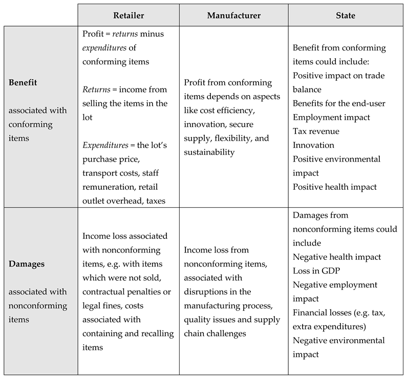
In acceptance sampling, the consumer is defined as the party which accepts or rejects the producer’s lot. The consumer may be a retailer purchasing commodities at a wholesale market, a manufacturer acquiring parts or a customs officer or food safety agent checking that legal limits for contaminants are not exceeded before admitting a lot at the border, etc... The following table provides different interpretations of benefit and damages for three different types of consumers.

Table 1.
The meaning of benefit and damages for different types of consumers.
 |
2.3. Mathematical Expression
The definition of utility makes it possible to apply a simple criterion in the design of acceptance sampling plans: select the plan which maximizes utility.
In order to express the utility function in mathematical terms, the following notation will be used:
| = benefit associated with one conforming item in an accepted lot | |
| = damages associated with one nonconforming item in an accepted lot | |
| = the testing and sampling costs per item |
All costs are expressed in terms . In other words, the common unit in which all the terms in the utility function are expressed is . For example, the damages associated with a nonconforming item could be 10 ; and the testing and sampling costs per item could be 5 . The values for and expressed in terms of will be referred to the cost structure.
The damages parameter can have different meanings. If there are no other costs and if there are no re-purposing options for items which are not sold, the value corresponds to the case that the only cost associated with a nonconforming item is the loss in income caused by its not being sold. A value such as corresponds to the scenario that, in addition to losses, there are additional costs associated with nonconforming items, such as costs associated with waste management. A value such as could reflect additional costs associated with environmental pollution, damage to the reputation of the retailer (dissatisfied customers taking their business elsewhere, tarnished public image) etc. Higher values such as or reflect substantial additional costs such as those associated with recalling a lot or healthcare costs. It may be difficult to quantify healthcare costs associated with nonconforming items (e.g. hospitalization costs due to the ingestion of contaminated meat). One approach could be to introduce an auxiliary unit such as = wages corresponding to a day’s work for an “average worker.” For example, if a brief stay in a hospital is quantified as 5 and if the profit (benefit ) associated with the item which caused the health issue (e.g. contaminated meat) is 0.1 , then is calculated as 50 .
Finally, we also introduce the following notation:
| Number of items in the lot | |
| Number of nonconforming items in the lot | |
| Sample size (i.e. number of items in the sample) |
The utility function is defined as follows:
In the case of an accepted lot, the utility function can be rewritten as
It should be noted that is an integer which, in general, remains unknown. The aim of the acceptance sampling procedure is to obtain an estimate of by means of a suitable (nonbiased) estimator for (or for the proportion of nonconforming items ), taking all prior information into account.
Historically, utility models underlying economic acceptance sampling often include terms for the effects of both lot acceptance and lot rejection, see Hald (1981) 5, Uhlmann (1982) 7 and Göb (1992) 6. These full utility models, often called cost or loss models, are usually articulated around a break-even point for the proportion nonconforming such that the utility of accepting the lot is greater than the utility of rejecting the lot for whereas the utility of accepting the lot is less than the utility of rejecting the lot for . For optimization studies based on such combined models, it is important to consider the so-called regret function, see Hald (1981) 5 and Uhlmann (1982) 8. As a function of the proportion nonconforming , the regret function is the difference between the actual costs and the unavoidable costs, calculated as the minimum of the acceptance costs and rejection costs. The sensible target of optimization procedures is the unavoidable loss expressed by the regret function. As demonstrated by Uhlmann (1981) 7, direct consideration of the utility often leads to unwelcome trivial optimum solutions.
3. Example
In order to illustrate the concept of utility as well as the coefficients for the benefit and damages discussed in the previous section, we consider the scenario where the utility is simply a given value rather than the expected value of a random variable. This is the case when no sample is inspected (and hence Bayesian inference is performed).
Consider the scenario where a retailer has accepted and purchased a lot of 2000 apples (400 kg) at a wholesale price of 600 €. The retailer expects to sell all apples at an average retail price of 4 € per kg. Total sales (if all apples are sold) for the lot will thus be 1600 €. Transport costs were 20 €. The retailer paid a salesperson 100 € for the day’s work.
The benefit for the entire lot (under the assumption that all the apples are sold) for the retailer is thus
A total of 100 apples (20 kg) had blemishes which resulted in being discarded (i.e. not sold). The retailer concludes that the damages caused by nonconforming items are .
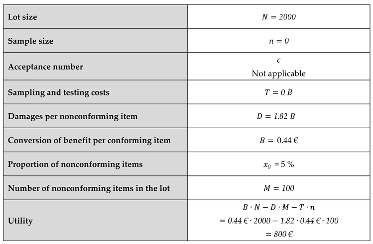
Benefit, damages and testing costs for the example
| Utility for a lot which has been accepted | = | benefit associated with an accepted lot (under the assumption that all items are conforming) i.e. returns minus expenditures | |
| minus damages associated with nonconforming items in an accepted lot | minus . | ||
| minus sampling and testing costs | minus . |
Accordingly, in this example, the utility for the lot is 800 €. Now, let us calculate the parameters and (we already know that ). The benefit per conforming item (apple without blemishes) expressed in Euros is
The damages associated with nonconforming items are
If the damages coefficient is expressed in terms of B, we have
The following table summarizes the example.
Table 2.
Summary of example of lot of 1000 apples.
 |
- Note 1
If the retailer purchases lemons instead of apples and if the lemons are displayed for purchase at the retail outlet during 10 days, then the retailer will worry about mold spread via contamination with neighboring spoilt lemons. If the lemons are sold individually and if the retailer observes that, on average, one spoilt lemon contaminates 5 neighboring lemons in the time span of 10 days, this state of affairs can be taken into consideration by multiplying the coefficient by 5.
- Note 2
If an intermediate distributor is involved in the purchase of a lot of 500 crates of 2000 apples ( apples), it is likely that the lot will be inspected prior to acceptance. In such a situation, will be nonzero.
- Note 3
If the aim is to use the utility in order to determine the acceptance sampling plan (sample size and acceptance number ), then the damages coefficient can be specified via the mean value of the prior distribution for the percentage nonconforming.
In order to illustrate this point, we start with the observation that, in the example above, at least 900 apples must be sold in order for the retailer to break even:
| Expenditures (Purchase price of the lot + transport costs + sales person remuneration) | 720 € |
| Retail price of apple | 0.8 € |
| Income from the sale of 900 apples (180 kg) | 720 € |
Accordingly, 1 maximum of 1100 nonconforming items (1100 apples with blemishes leading to discarding) can be tolerated in order to break even. This corresponds to a maximum of 55% for the percentage nonconforming.
If the retailer works with a prior distribution for the percentage nonconforming whose mean value is 10% (i.e. well below the maximum of 55%), then D can be determined as follows. First, we note that the percentage nonconforming corresponds to . In the absence of testing costs, the utility is simply
Setting (i.e. lot acceptance in the sense of breaking even), we obtain the following expression for the damages coefficient
If is expressed in terms of , then this simplifies to
For (the prior which the retailer is working with), we thus obtain .
- Note 4
It is important to understand the impact which has on the utility. In particular, in the absence of sampling and testing costs, the value means that one single sold item is sufficient to have a positive utility.
Indeed, for and we have
Now, in the example of the lot of 2000 apples, the lot has already been accepted and purchased and the proportion of nonconforming items can be empirically determined by 100 % inspection of the lot. In other words, in such a case, is an empirically determined value rather than a random variable (hence the notation with the subscript). However, the aim of the utility approach is to determine sample size and acceptance number—in other words to design the acceptance sampling plan—prior to lot inspection. For this reason, in the following, the empirically determined value will be replaced with a random variable . This random variable is the prior distribution and reflects the consumer’s best understanding of the quality of the lot. An immediate consequence of introducing the random variable for the proportion nonconforming is that the calculation of the utility will involve integrating across all values for , weighted by the distribution function (the prior). Integrating in this manner gives a slightly different meaning to the utility: instead of an empirical value corresponding to a given lot, it is now an expected value, in the probabilistic sense. The calculation of the utility as the expected value of a random variable is described in the following sections.
4. Notation and Preliminary Considerations
4.1. General Case
The plans described here are intended for the inspection of isolated lots, in the sense that no switching rules are applied and that a new acceptance sampling plan must calculated for each new inspection. This does not mean that each lot must come from a new supplier. Rather, it is assumed that the consumer has had some experience with the supplier of the lot currently under inspection. Hence, it is reasonable to assume that available information regarding lot quality is available.
The proportion nonconforming is modelled as a (continuous) random variable denoted which takes on values in the interval [0,1]. It is assumed that a prior distribution for is available. The density function of this prior is denoted with denoting the vector of hyperparameters.
The testing outcome during lot inspection is the number of nonconforming items in the sample of items. This outcome is a (discrete) random variable denoted with realizations which takes on integer values between 0 and .
Further below, the posterior distribution will also be considered. When it is necessary to distinguish the two random variables and , they will be denoted and , respectively.
The density function of the joint distribution of and is denoted .
We have
For a given the mean of the posterior distribution can be calculated as
For the marginal probability we have
For the product we have from Equation 4
4.2. The Case that the Prior is a Beta Distribution
The above mathematical expressions are valid independently of the choice of prior .
In this section, we provided expressions for joint distribution , the posterior mean and the marginal probability for the case that the prior for the proportion nonconforming is a beta distribution, i.e. , and for the case that the number of nonconforming items in a sample of items follows a binomial distribution.
For the joint distribution, we have from Equation 3 (first equality)
where denotes the binomial probability mass function, i.e. the probability of observing events with a probability of occurrence of in trials.
For nonconforming items in a sample of items, from the first equality in Equation 4, the mean of the posterior distribution is
where .
Finally, the marginal probability is obtained by integrating Equation 7 over all values of :
- Note
In the following, many examples are based on the beta prior. This is suitable for modelling the quality of a process. For an individual lot, the hypergeometric distribution is more appropriate. The calculations with the hypergeometric distribution will be discussed in a subsequent article.
5. Estimation of the Utility Under the Prior Distribution
Lot acceptance is conditional on the following decision rule:
Accept the lot if , where denotes the acceptance number.
Both the sample size and the acceptance number are determined by maximizing the expected value of the utility (see Equation 1)
The expected value of the utility for an acceptance plan and a given prior is denoted
We have
Let
and let
Using this notation, we have
Sample size and acceptance number are determined by maximizing .
6. Excursus: Correspondence between the Approach Described Here and the Approach Described in Hald
We start by recalling the three cost functions defined in Section 1.4 in Hald (1981) [5]. In doing so, we use Hald’s notation; in particular the proportion nonconforming is denoted , where denotes the number of nonconforming items (Hald: “defective units”) in the lot and denotes the lot size (as in the present paper).
For the calculation of Bayesian plans, Hald uses the following cost function (see Section 7.3 in Hald (1981) [5]):
where denotes the acceptance probability for a lot with defect rate .
With the present paper’s cost parameters, this can be rewritten as
Hald then integrates over the prior distribution for to obtain the cost function as a function of , and :
The cost function ist near identical to the negative of the expected utility described above (see Equation 12); the only difference is the factor instead of .
For a given lot size , the Bayesian sampling plan is then obtained by minimizing the costs with respect to . Clearly, this is equivalent to maximizing the utility. In can be concluded that the approach presented here can be subsumed within Hald’s theoretical framework for Bayesian acceptance sampling plans.
Note regarding the regret function
Hald defines the unavoidable costs at quality level as
The regret function as a function of is then defined as the actual costs at minus the unavoidable costs at (see Section 1.4 in Hald (1981) [5]).
In Section 7.3, after discussing the cost function , Hald explains that the same plans can be obtained by minimizing the standardized average regret function, defined as
where the average minimum costs are defined in Section 1.7.5 as
(for the case that the prior for the parameter p is a beta distribution) and the parameters and are defined above in Table 3 (and in the present paper’s notation).
In the present paper’s notation, we have
and hence
and thus
In the following section, diagrams of utility and regret functions for different values of and are provided.
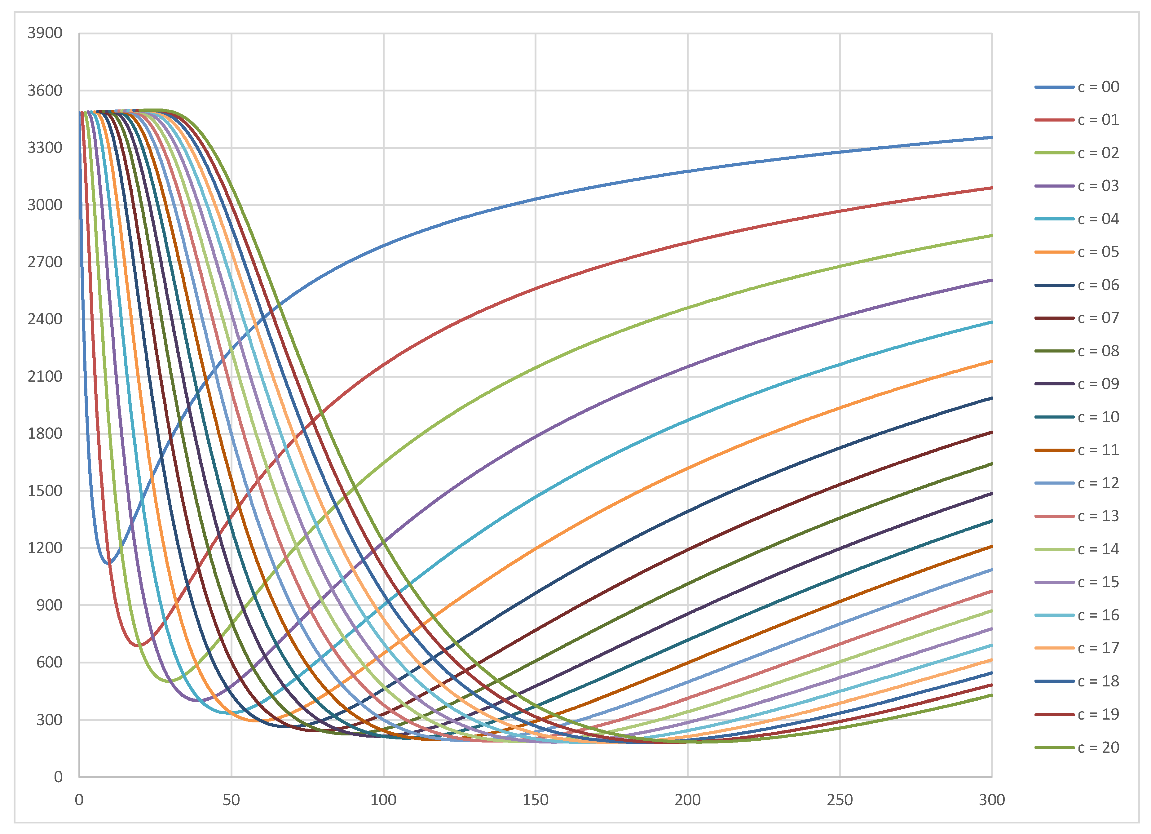
6. Utility and Regret Curves
The following diagrams show utility curves for the prior Beta(1,9) and for the prior Beta(0.5,0.5).
The -axis shows the sample size and the -axis shows the expected utility . There is a separate curve for each acceptance number .
As can be seen, the utility values for the more optimistic prior are greater (maximum around 33000 ) than for the non-informative prior (maximum around 12600 ).
The following diagram shows utility curves for the prior Beta(1,9), lot size = 100000 and cost structure and . The optimum plan is , (utility = 33043 ).
- Note
For each acceptance number , the curve has a clear maximum value (at the optimal sample size ). For example, for the curve, the optimal is 59. However, for a given sample size , the optimal may not be unique. For example, for , the maximum utility value 31490.86 is achieved at both and . Across and , however, the maximum utility value is unique—though the utility values tend to reach a plateau around this maximum value. This motivates the following procedure: we propose to consider plans whose utility lies within 10% of the maximum utility. This will allow a considerable reduction in sample size while maintaining a negligible impact on utility.
For instance, the maximum utility for the Beta(1,9) prior is 30457 . Subtracting 10% of this maximum value, we obtain 29739 . The curve exceeds this value at . Hence the , plan can be replaced with , .
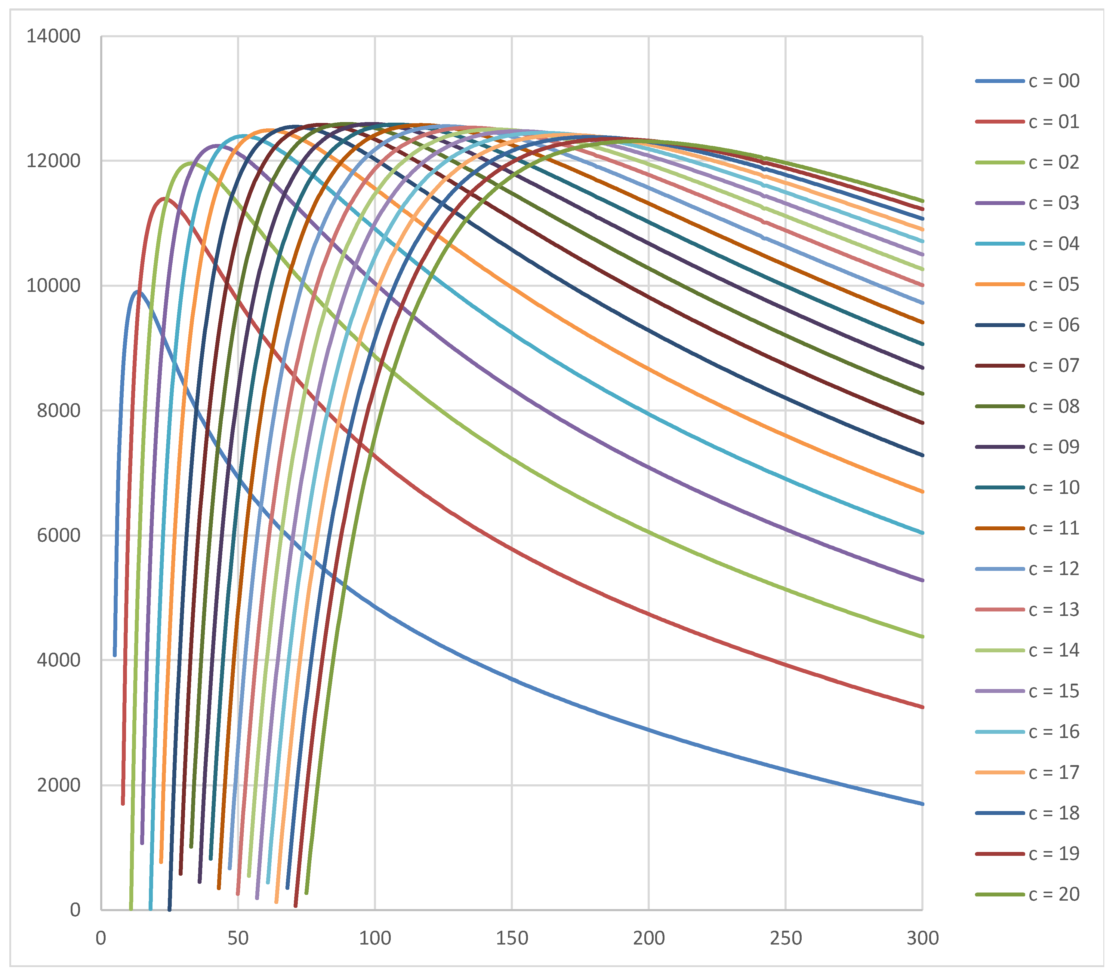
The following diagram shows the utility curves for the Jeffreys prior Beta(0.5,0.5), which represents the case that no prior information is available (noninformative prior). As in the previous diagram, the lot size is 100000 and the cost structure is and . The optimum plan is , (utility = 12592 ).
Finally, we also show the regret curves for the Beta(1,9) prior. This should be compared to Figure 1. The optimal sampling plan (corresponding to the minimal regret value) is the same:
Figure 1.
Utility curves for different acceptance number c values as a function of sample size n for the prior Beta(1,9), lot size N = 100000 and the cost structure D = 10 B and T = 5 B.
Figure 1.
Utility curves for different acceptance number c values as a function of sample size n for the prior Beta(1,9), lot size N = 100000 and the cost structure D = 10 B and T = 5 B.
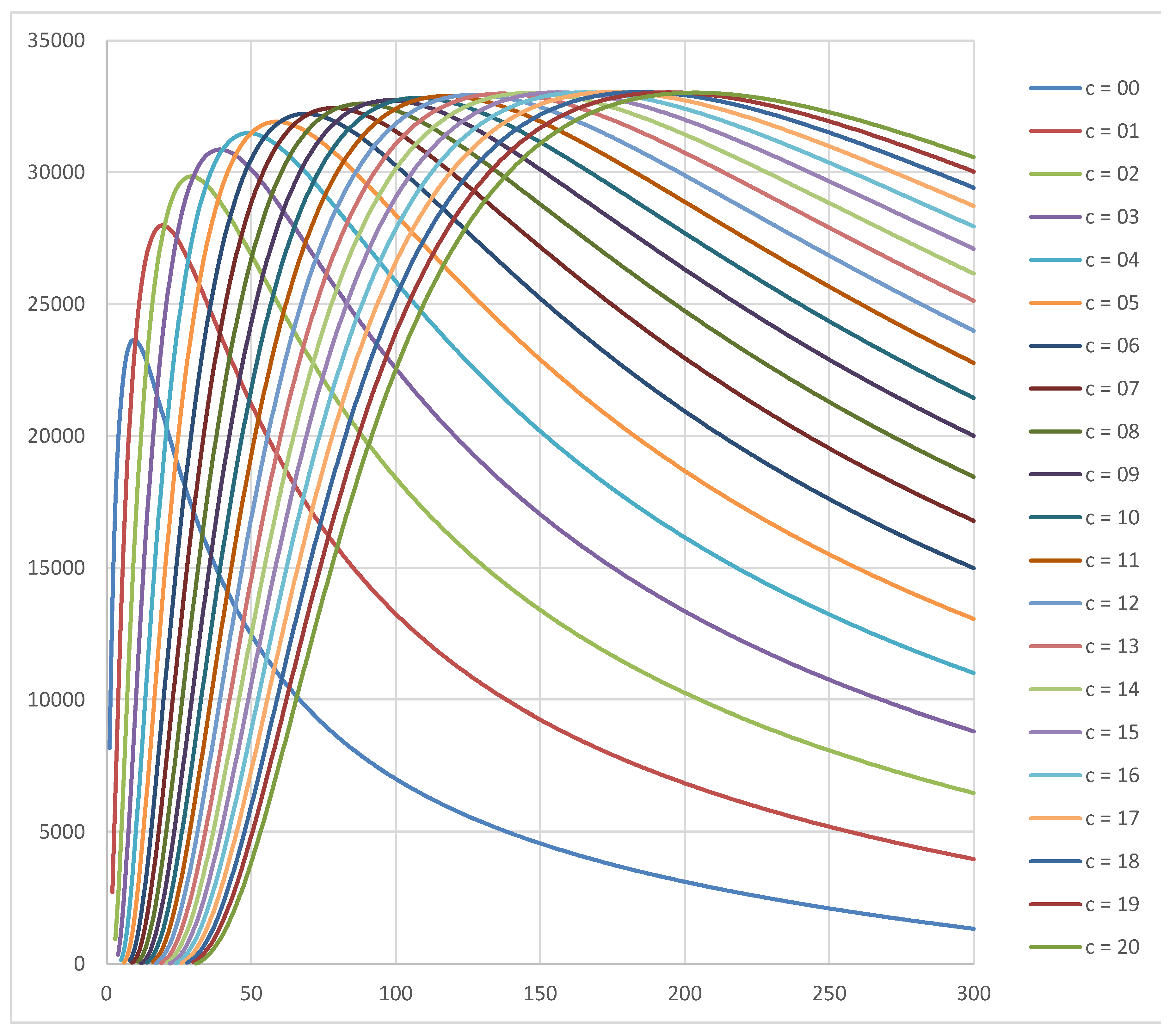
Figure 2.
Utility curves for different acceptance number values as a function of sample size for the prior Beta(0.5,0.5), lot size N = 100000 and the cost structure = 10 and = 5
Figure 2.
Utility curves for different acceptance number values as a function of sample size for the prior Beta(0.5,0.5), lot size N = 100000 and the cost structure = 10 and = 5
The following diagram shows regret curves for the prior Beta(1,9), lot size = 100000 and cost structure and . This should be compared to Figure 1. Just as in the case of maximizing the utility function, minimizing the regret function yields the optimum plan , (regret = 33043 ).
Figure 3.
Regret curves for different acceptance number values as a function of sample size for the prior Beta(1,9), lot size = 100000 and the cost structure = 10 and = 5
Figure 3.
Regret curves for different acceptance number values as a function of sample size for the prior Beta(1,9), lot size = 100000 and the cost structure = 10 and = 5
7. Calculation of the Sample Size and the Acceptance Number
- Outline
The procedure is as follows:
Step 1: For each , determine the optimal acceptance number and the corresponding utility .
Step 2: Determine the maximal utility value Step 3: Select the minimum for which .
- Note
The rationale for step 3 is based on the discussion at the end of Section 0.
- Procedure for Step 1
We start with the expected utility for an acceptance plan and a prior (see Equation 13). The following notation is introduced:
where
and, for a given integer ,
The question is how to determine the optimal acceptance number for a given sample size .
For nondegenerate distributions, the sequence is monotonically decreasing. The optimal acceptance number can thus be determined via the simple rule
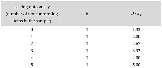
- Example
The following table illustrates the rule for the determination of (see Equation 15). We start by noting that Equation 15 is equivalent to requiring that for , we have
Table 4.
Calculation of acceptance number for the sample size = 3. The lot size is = 1000, the cost structure and and the prior is Beta(1,9). The coefficient is less than for all outcomes and the acceptance number is thus determined as .
Table 4.
Calculation of acceptance number for the sample size = 3. The lot size is = 1000, the cost structure and and the prior is Beta(1,9). The coefficient is less than for all outcomes and the acceptance number is thus determined as .
 |
9. Posterior Utility
In addition to the prior utility, it is possible to define a posterior utility. The posterior utility is defined for a given testing outcome during the inspection of a given lot. In particular, the posterior utility plays no role in the calculations of an optimal plan. Rather, the posterior utility can only be calculated once the acceptance sampling plan has already been specified.
If the testing outcome is (corresponding to lot rejection), the posterior utility is
For (i.e. the lot is accepted) we have and the posterior utility is thus defined as
10. Evidence-Based Calculations
The main drawback of the “naïve” posterior expected values used in the Bayesian approach described above is as follows: the prior distribution and the distribution of the observations are combined in the calculation of the posterior no matter how much they deviate from one another. If a very optimistic prior, e.g. a beta distribution with and , were updated on the basis of test results from a sample of 20 items in which 10 of the items tested were nonconforming, the naive Bayesian would calculate a posterior beta distribution with and . The expected value of the posterior distribution would be , and one would conclude that the actual proportion nonconforming of the lot lies in this region. The frequentist, on the other hand, would conclude that the underlying prior does not match the very poor sample results and would check this with an appropriate statistical test.
The layman would react skeptically to acceptance plans obtained via the “naïve” Bayesian approach. Indeed, given a Beta(,) prior, a slight increase in the parameter is often sufficient to obtain a plan with (i.e. accept without testing). In practice, it is often necessary to check the assumption encapsulated in the prior distribution.
In order to overcome this shortcoming, we propose to use a hierarchical Bayesian model for the prior.
The approach is illustrated for the case of the beta prior and the binomial distribution. In this case, the hierarchical model can be expressed as the mixture of two beta distributions. The prior takes the following form
The model in Equation 17 is a hierarchical Bayesian model where the first-level distribution is governed by the hyperparameter and the second level is governed by the four parameters and . It should also be noted that the following shorthand notation is used in Equation 17:
where denotes the beta density function and denotes the binomial probability mass function, i.e. the probability of observing events with a probability of occurrence of in trials.
The parameter will also be referred to as the “mixing parameter” of the two beta distributions Beta and Beta.
Beta encapsulates available prior information—i.e. Beta is the presumptive prior—while Beta represents a noninformative prior, e.g. the Jeffreys prior Beta. Beta thus plays the role of a check on the presumptive prior Beta. The mixing parameter can be seen as the parameter of a higher-order prior for the two beta distributions, referred to as and . In this interpretation, we have and . In the following, we will set . This expresses a confidence level of 80% in our prior information .
The question is: how much evidence do nonconforming items in a sample of items provide for . This motivates the following definition of the evidence:
The evidence is calculated as follows:
Finally, it is important to consider the posterior distribution of the mixture distribution defined via Equation 17. It can be shown that this posterior distribution is also a mixture distribution of two beta distributions. The posterior beta hyperparameters are as follows:
The posterior mixture parameter is calculated as follows:
The expected value of the posterior mixture distribution is
The evidence-based approach can easily be applied by replacing the expressions for and in the calculation of (see Section 0) by those in Equation 17 and in Equation 22.
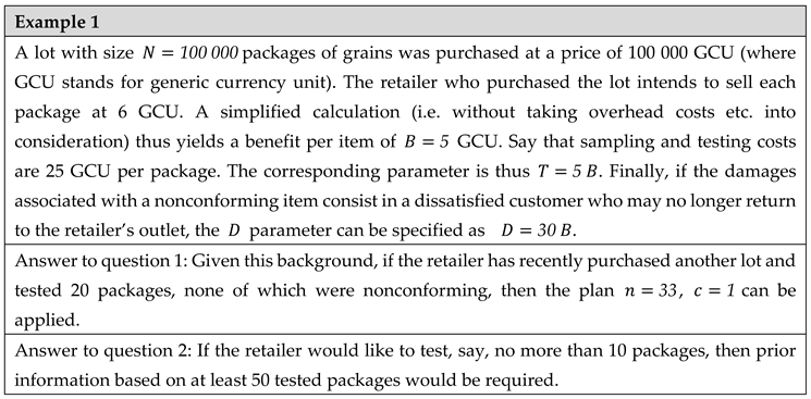
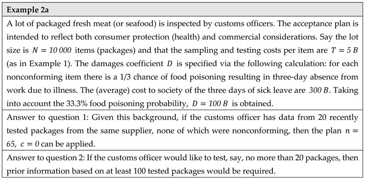
11. Standard Plans
This section provides tables with standard plans for the practitioner. It is assumed that there is no inspection error and that prior information is available in the form of results from previous testing performed on items from the producer of the lot currently under inspection. It is assumed that these previous tests have been performed recently—say, within the previous 2 or 3 months. In the tables, the results from previous testing are represented via the pair with denoting the number of items previously tested and denoting the number of nonconforming items from these recent tests.
For a given pair (, ), the plans are calculated on the basis of a Beta() prior for the proportion nonconforming where
The pair stands for the absence of any prior information. This scenario is represented as the first row in each of the tables. The corresponding standard plans are based on the noninformative Jeffreys prior, i.e. the Beta(0.5,0.5) distribution.
The standard plans can be used to answer two questions.
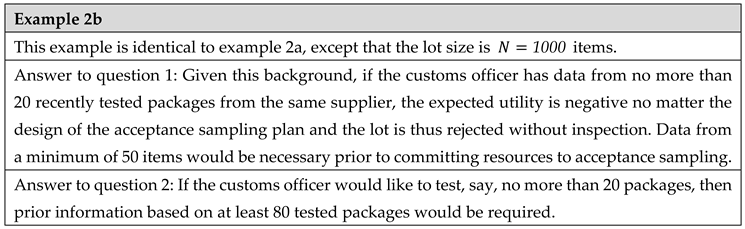
Question 1: Given prior information, a cost structure and a lot size, which acceptance sampling plan should be applied?
Question 2: Given a cost structure and lot size, what type of prior information is required in order to achieve an acceptance sampling plan whose workload is acceptable (or indeed, for it to be worthwhile to perform acceptance sampling at all)
In order to illustrate the use of the standard plans to answer these two questions, consider the following examples.
 |
 |
 |
- Notation
The following notation is used in the tables:
| Previous testing / prior information The number of items tested prior to the current lot inspection |
|
| Previous testing / prior information The number of nonconforming items |
|
| Lot size | |
| Damages/losses/costs per nonconforming item (expressed in terms of the benefit per item ) |
|
| Sampling and testing costs per item (expressed in terms of the benefit per item ) |
|
| a | Accept without testing |
| r | Reject without testing |
| Acceptance sampling plan with sample size acceptance number |
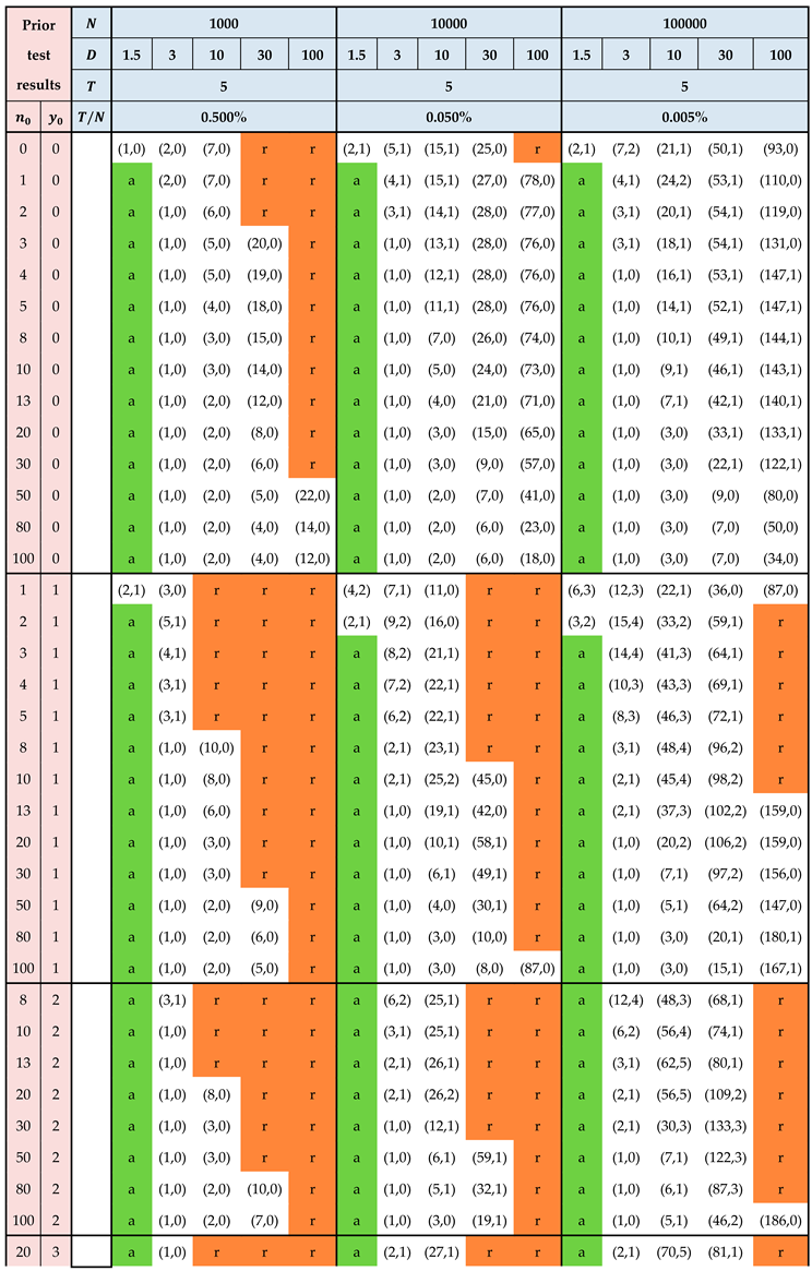
Table 5.
Standard plans for testing and sampling costs
 |
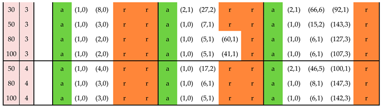 |
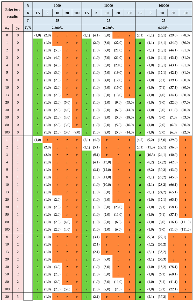
Table 6.
Standard plans for testing and sampling costs
 |
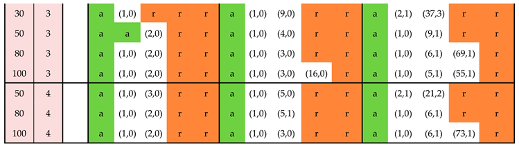 |
- General notes
Note 1: As the lot size increases, the sample size also increases, but at the same time, it becomes “easier” to justify investing resources in lot inspection—i.e. plans are available at lower values (less prior information is required). This is due to the increase in total benefit due to the increased lot size.
Note 2: For a given cost structure and lot size, the sample size is less for than for . On the other hand, a higher value is required prior to committing resources to acceptance sampling for .
Note 3: The ‘r’ entries (highlighted in red in the table) indicate that the lot should be rejected without testing. This should be interpreted as follows: given the testing costs and the damages associated with nonconforming items, it only makes sense to invest resources in lot inspection given a minimum level of confidence in the lot quality. This minimum level of confidence is codified via the pair. For example, for a relatively small lot () and a very high value for (, reflecting for example a health hazard in connection with nonconforming items), it only makes sense to conduct acceptance sampling if the prior information is based on at least 50 previously tested items with zero nonconforming results.
If the consumer rejects the lot without testing, the producer has the following options:
- Increase the lot size . As seen in the standard plans, a larger lot size translates to higher income for the consumer, thus lowering the threshold for investing resources in acceptance sampling.
- Decrease the purchase price of the lot. This is tantamount to increasing the parameter , which, in turn, will result in lower values for and . This will lower the threshold for investing resources in acceptance sampling.
- Develop test methods which are cheaper to apply. This option will result in a decrease in the parameter, thus lowering the threshold for investing resources in acceptance sampling. An important caveat here is that the performance of the new method must be at least as good as that of the original method.
- Technical notes
Note 1: The standard plans were calculated via the procedure described in Section 0 with the evidence-based modification from Equation 22. The 10% approximation was also applied, see the Note after Error! Reference source not found..
Note 2: We define the ratio = (or if is expressed in terms of ). The probability that the percentage nonconforming exceeds is an interesting pendant to the consumer’s risk in the ISO 2859 series of standards. See the discussion in Hald 5.
Note 3: The sample size increases with as long as the mean value of the beta distribution corresponding to is less than the ratio = (or if is expressed in terms of ). When this mean value is greater than , the sample size decreases as increases. This can be explained as follows: if the mean value is less than , it is unlikely that utility will be positive, and the natural tendency of the model is to resist investing resources in lot inspection. This resistance decreases as the prior becomes more optimistic. By contrast, if the mean value is greater than , then it is likely that the utility will be positive, and the natural tendency of the model is to invest resources in lot inspection. As the prior is becomes more optimistic, fewer resources are required.
Note 4: The standard plan for , , , , is “accept” rather than (1,0). This anomaly may possibly be related to rounding issues.
12. Discussion
12.1. Further Work
Utility is always connected to a certain perspective. The present paper focuses on the consumer’s perspective and a utility concept has been developed which is general enough to be applied independently of whether the consumer is a private-sector retailer or a state agency such as a consumer protection agency or customs office. As discussed above, the approach presented here must be extended to reflect both the consumer’s and the producer’s point of view. The basic theory has already been developed and is described in the Lindley and Singpurwalla paper 4.
In the present paper, only lots consisting of discrete items have been considered. Accordingly, the approach described here allows the calculation of acceptance sampling plans for inspection by attributes, where the acceptance criterion is expressed in terms of the number of nonconforming items in the sample taken from the lot. The approach presented here can be extended to inspection by variables and to lots consisting of bulk material, where the acceptance criterion is expressed in terms of the lot mean. This will be discussed in a subsequent paper.
Similarly, the present paper does not address the issue of measurement or inspection error. This question must also be addressed in future work.
Finally, the calculations in the present paper are based on the assumption that test outcomes follow the binomial distribution. Strictly speaking, this is only appropriate in connection with a process rather than a lot. It is thus desirable to adjust the calculations described here for the case that outcomes follow the hypergeometric distribution. Similarly, the factor rather than was used in the utility function for the parameter . Strictly speaking, this is more appropriate for a process than for a lot.
12.2. Conclusions
As we have seen in this paper, it is possible to design an acceptance sampling plan on the basis of a utility function and prior distribution. By shifting from the question of risk reduction to the question of utility maximization, it is possible to considerably reduce the sample size in the design of acceptance sampling plans. In addition to reducing the lot inspection workload and costs, the utility approach also presents advantages insofar as the risk-paradigm is replaced by procedure in which real costs are internalized. Many regulations prioritize minimizing a certain type of risk. However, focusing on a single type of risk often results in too narrow a perspective for complex decision making. In a more holistic approach, all relevant benefits and costs are weighed against each other. This is precisely what the utility approach aims to achieve. For example, from the point of view of a national economy, a more differentiated decision-making will consider the CO2 footprint of combustion engines in a comprehensive costs and benefits calculation rather than issuing a blanket ban. In guidelines for many key societal activities such acceptance sampling plans, contaminant monitoring programs, method validation and proficiency testing, laboratory accreditation etc., it is essential that bureaucratic and administrative costs be correctly accounted for in utility calculus.
Admittedly, some damages or costs—such as reputational loss or healthcare costs—are difficult to quantify. In such cases, pragmatic procedures must be developed. For example, calculating the benefit associated with an accepted lot from the point of view of a state is not always straightforward. Indeed, from the point of view of the state, some of the positive aspects of a successful commercial transaction may be intangible or difficult to assign a precise monetary value to. In such cases, as a rule of thumb, it is suggested to use the lot’s purchase price.
As can be seen in the standard plans, the acceptance sampling plan depends very much on the lot size. Indeed, a large lot size translates to an increase in total benefit, thus impacting the calculation of utility. For example, for the cost structure and , and for the prior information , there is an acceptance plan (i.e. it makes sense to invest resources in lot inspection) only for the lot size . Indeed, for the lot size and the lot size , the utility approach results in the decision to reject the lot without testing. These considerations show the extent to which the acceptance samplings plans (including the decision to reject without testing) reflect the cost structure internalized in the parameters of the utility model.
There are three takeaways from this for the consumer.
The first is that the consumer can perform some preliminary calculations and inform the producer prior to the lot being shipped that, given the cost structure, the transaction is only commercially viable for a minimum lot size.
The second is that, in certain circumstances, it could lie in the interest of the consumer to “pretend” that the lot size is greater than it actually is in order to achieve a viable acceptance sampling plan. For instance, consider the case that an importing country is initiating commercial relations with a new supplier and that the first lot—intended as a trial—is smaller in size than subsequent “routine” lots would be.
The third and last takeaway is that an indispensable condition for achieving plans which successfully balance the producer’s and the consumer’s interests is transparency. For instance, the producer must be able to ascertain whether the consumer intends to reject without testing or to apply an acceptance sampling plan prior to shipping the lot. Indeed, this last take away leads directly to the question whether it is possible to combine or couple utility functions representing the consumer’s and the producer’s perspectives so as to achieve a broader notion of utility representing, as it were, a win-win situation for both parties to the transaction.
References
- ISO 2859-1:1999 Sampling procedures for inspection by attributes. Part 1: Sampling schemes indexed by acceptance quality limit (AQL) for lot-by-lot inspection.
- ISO 3951-1:2022 Sampling procedures for inspection by variables. Part 1: Specification for single sampling plans indexed by acceptance quality limit (AQL) for lot-by-lot inspection for a single quality characteristic and a single AQL.
- Lindley D, Singpurwalla N. On the evidence needed to reach agreed action between adversaries, with application to acceptance sampling. Journal of the American Statistical Association, Vol. 86, No. 416 (Dec., 1991), pp. 933-937.
- Lindley D, Singpurwalla N. Adversarial life testing. J. R. Statist. Soc. B (1993) 55, No. 4, pp. 837-847.
- Hald A (1981). Statistical Theory of Sampling Inspection by Attributes. Academic Press Inc, London New York.
- Göb R. α-Optimal sampling plans for lot-by-lot defects inspection. Metrika (1992), Vol. 39, pp. 269-316.
- Uhlmann W. Zum Minimax-Prinzip in der statistischen Qualitätskontrolle. Metrika (1981), Vol. 28, pp. 203-206.
- Uhlmann W. Statistische Qualitätskontrolle, 2nd ed. Teubner Verlag, Stuttgart (1982).
- Uhlig S, Colson B, Kissling R, Ellis S, Hicks M, Vandenbemden J, Pennecchi F, Göb R, & Gowik P (2024). Acceptance Sampling Plans Based on Conformance Probability—Inspection of Lots and Processes by Attributes. Preprints. [CrossRef]
Table 3.
Cost functions corresponding to the model described in Hald (1981).
| Costs per item of | Hald’s cost functions | Our approach in Hald’s notation |
| Rejection | , i.e. | |
| Acceptance | and , i.e. | |
| Sampling inspection | and , i.e. |
| 1 | This is not necessarily the case if the switching rules are applied. |
| 2 | The diagonal in Table 2-A between sample size code Q / AQL 0.01% and sample size A / AQL 6.5%. |
| 3 | Some of these Bayesian risks had already been discussed in the literature and in JCGM 106. See [9] for details. |
| 4 | Statistical arguments alone (such as the question of statistical significance) often constitute an inappropriate basis for decision making. Indeed, with a sufficiently high sample size, it will always be possible to obtain statistically significant results. But this seldom the question which is actually relevant. |
| 5 | For the sake of simplicity, neither overhead costs (associated with the retail outlet) nor taxes are included here. |
Disclaimer/Publisher’s Note: The statements, opinions and data contained in all publications are solely those of the individual author(s) and contributor(s) and not of MDPI and/or the editor(s). MDPI and/or the editor(s) disclaim responsibility for any injury to people or property resulting from any ideas, methods, instructions or products referred to in the content. |
© 2025 by the authors. Licensee MDPI, Basel, Switzerland. This article is an open access article distributed under the terms and conditions of the Creative Commons Attribution (CC BY) license (http://creativecommons.org/licenses/by/4.0/).
Copyright: This open access article is published under a Creative Commons CC BY 4.0 license, which permit the free download, distribution, and reuse, provided that the author and preprint are cited in any reuse.


