
Submitted:
18 April 2025
Posted:
21 April 2025
You are already at the latest version
Abstract
Self-adaptive systems play a crucial role in the industrial world due to their ability to make corrections following environmental destabilization. In this paper we addressed the implementation of a machine learning approach which allows the detection of environmental hazards for the adaptation of information systems. We used internet connectivity data, which we collected from different networks, to train the model. We carried out these processes based on five machine learning algorithms, namely: XGBoost, Random Forest, SVM, Decision tree, K Neighbors. The results obtained by its algorithms in terms of test accuracy are 99.95% for XGBoost, Random Forest Decision tree, and 97.62% for SVM and 99.80% for K Neighbors. In terms of train accuracy are 100% for XGBoost, Random Forest Decision tree, and 97.74% for SVM and 99.84% for K Neighbors. In terms of F1-score are 99.95% for and 97.80% for K Neighbors. In terms of precision are 99.95% for XGBoost, Random Forest Decision tree, and 97.75% for SVM and 97.81% for K Neighbors. In terms of recall are 99.95% for XGBoost, Random Forest Decision tree, and 97.62% for SVM and 97.80% for K Neighbors. We also carried out a comparative analysis of the results obtained by each of the five algorithms, based on the following performance indicators: accuracy, F1-score, precision, Recall.
Keywords:
Artificial intelligence
; Machine Learning
; Adaptive Systems
; Computer Science
; Anomaly detection
1. Introduction
Adaptive systems are now crucial for increasing service effectiveness across a range of industries[1]. This is due to the possibility of technical environments being unstable and heterogeneous sources for systems. Any system that has the ability to adjust to errors that happen in its technological environment is considered adaptable. Either the system’s configuration or its structure can be changed to accommodate adaptation[2]. System adaption may be made possible by external devices. A system is considered self-adaptive when it controls the adaptation process on its own[3]. Adaptive capabilities are necessary for information systems, which is a difficult but crucial task in the engineering process. As a result, it is crucial to concentrate on enhancing ways for implementing adaptive capabilities and perhaps investigating new techniques based on the requirement for improvement. In information systems, adaptability is typically controlled through a control loop[4]. This system’s architecture is broken down into several sections and elements, each of which plays a particular purpose in the adaption process. The adaptive system interacts with its environment on a high level to stay aware of any changes. Nevertheless, as we will see in more detail later, at a lower level, the core parts of the adaptive system perform this function explicitly.
We shall describe the key elements of the adaptation process in the sections that follow. In the case of an adaptive web application, the main system is in charge of granting user requests or wishes, such as giving requested pages. The environment consists of systems, outside elements, and data that are constantly in communication with the adaptive system. The system evaluates whether adaptation is required and, if so, what form it should take using input from the environment. The following figure gives an overview of the architecture of an adaptive system and its operating environment.
Figure 1.
Adaptive system architecture.
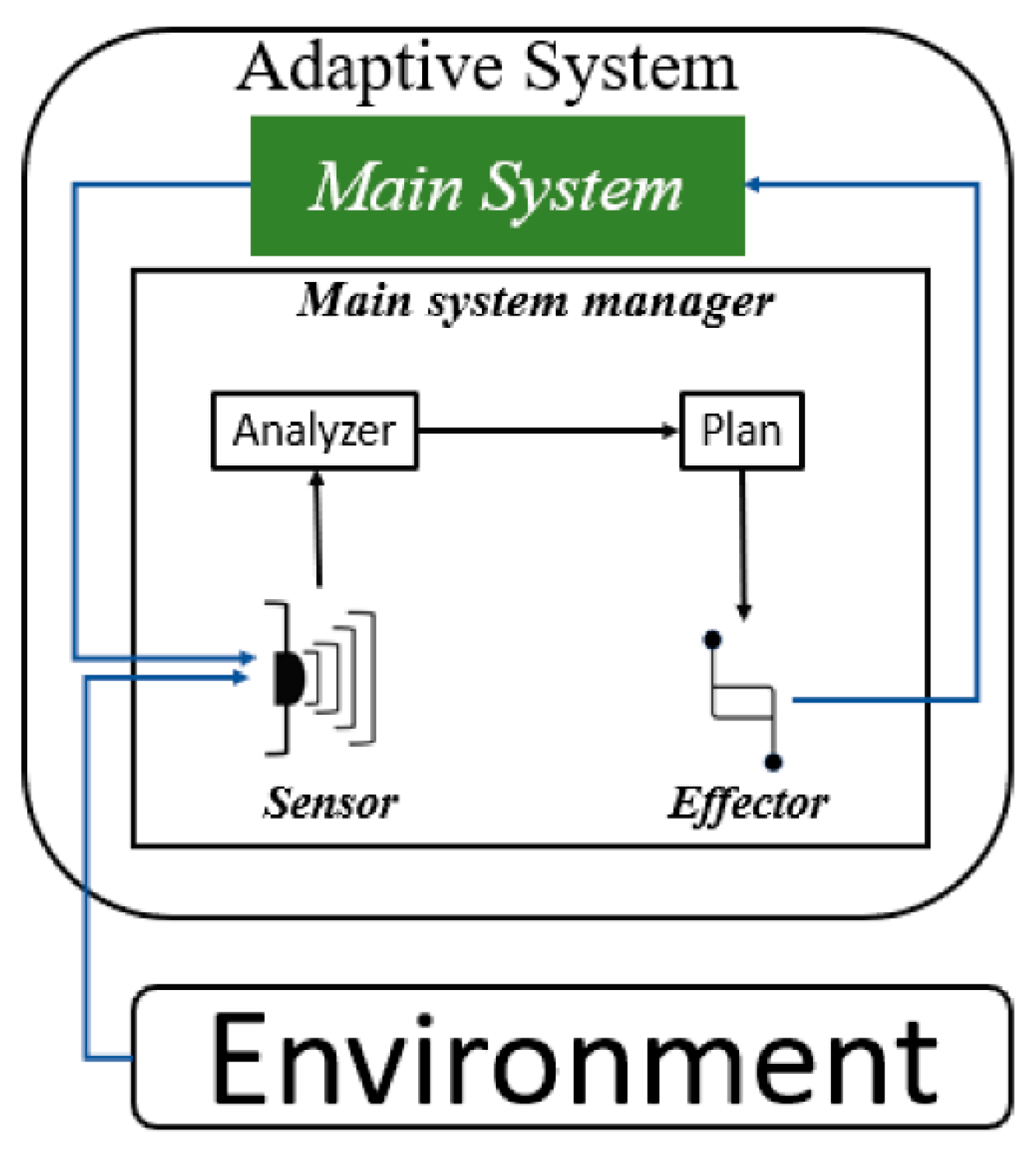
The technological components of adaptation fall within the purview of the main system management. This area is where the environment is sensed, responses are planned, and activities are carried out in response to environmental anomalies. The manager is made up of a number of parts, including the sensor, analyzer, plan, and effector, each of which has a distinct function.
The sensor component keeps watch on the environment of the system and keeps an eye out for any unusual occurrences. It notifies the analyzer of any such changes so that it can determine the nature of the abnormality. The analyzer communicates the findings to the plan component after it has finished its analysis.
The main contribution of this paper is the implementation of a machine learning model that will help detect environmental risks of a system and trigger the adaptation process. To do this, this article contributes to the establishment of a set of data that we have collected ourselves. Then an analysis of this collected data was carried out, before using it in the training and testing of this model.
In order to better arrange the rest of this paper, the second portion will concentrate on the work that is connected. In Section 3, the following classifiers are discussed: random forest, K-neighbors, support vector machine, decision tree, and XGBoost. In the fourth section, the results of the experiments and comparisons are discussed. Finally, Section 5 concludes with the conclusions.
2. Related Work
A great deal of research has been done in this area as a result of the scientific community’s significant interest in it. Due to the fact that there are still many unresolved parts of the issue it raises, this topic is still important today and draws new researchers.
Many researchers have taken on this topic and offered numerous strategies to streamline the management of adaptation in information systems. Model-driven engineering, which is increasingly employed in computer engineering, is one strategy they use. They also use the machine learning model creation process.
Sousa et al. (2013) outline a model-based method for creating adaptive systems in their study. This strategy provides a high level of abstraction, which makes it simpler to use and integrate with other strategies. From a technical perspective, it can be referred to as a modeling language because it is primarily concerned with the design process. Bachir et al. (2020) present a model-based method that gives a modeling environment to enable the system adaption process and is motivated by the Model-View-Controller (MVC) pattern’s behavior. Engineers can specify how the adaptation of an information system should be managed using the tools provided in this environment to articulate the adaptation requirements of the system. In order to create self-adaptive systems, Cetina et al. (2008) suggest a model-driven methodology that makes use of execution models. Their method comprises model-based components to handle scenarios of pervasive system evolution and offers tools to manage the adaptation of pervasive systems. Also, they separate the structure of the system from the process of adaptation, allowing for the replacement of outdated, faulty parts with new ones to guarantee proper system operation. In order to specify the entire structure of an adaptive system, Bachir et al. have proposed a different approach known as the models-based approach. The authors advise creating a UML profile that makes use of stereotypes to express the different parts of the system adaption process in an understandable and succinct way as a way to put this approach into practice. Van Der Donckt et al. (2019).’s alternative method offers two ways to deal with the adaptation mechanism: examining adaptation costs and condensing adaptation areas. While many approaches concentrate on the advantages of adaptation in a system, they frequently ignore the costs involved, which may cancel out any gains obtained from adaptation. The authors present CB@R (Cost Benefit analysis@Runtime), a model-based technique for making runtime decisions in self-adaptive systems that takes into account both the advantages and disadvantages of adaptation as crucial deciding variables, to address this problem. On the other side, they also examine the self-adaptive systems’ adaptation space, or the variety of viable adaptation alternatives. Yet, given time and resource limits as well as the potentially huge number of adaptation choices, it is frequently unfeasible to analyze the whole adaptation space. The authors propose a method that uses automatic learning to extract a subset of pertinent adaptation alternatives based on the current circumstance, incorporating the learning process into the control loop, to address this issue. The control loop is ultimately in charge of analyzing the subset of adaption possibilities and selecting the best one. Using an actual Internet of Things (IoT) application, the authors evaluated their methods, CB@R and the learning methodology. In order to set a theoretical limit on the influence of machine learning when applied to decision-making by a self-adaptive system based on its verification results, Gheibi et al. (2021) adopted a number of concepts and theorems from computational learning theory (CLT), as put forth by Angluin (1992). To aid in self-adaptive decision-making, they pair a form of learner, specifically linear regression, with a type of checker, specifically statistical model checking. Their main goal is to establish a theoretical upper bound on the assurances offered by the combination of statistical model checking and linear regression for decision-making in self-adaptation. An experimental examination is carried out utilizing the DeltaIoT artifact scenario to determine the theoretical limit (Iftikhar et al., 2017). Those investigated methods aimed to identify modeling techniques or languages that could cover all stages of the system adaptation process, which made them difficult to manage due to their broad scope. In contrast, our approach focuses on a specific stage of the system adaptation process and incorporates a machine learning approach that allows for dynamic operation, making it more practical. The previous model-driven approaches were mostly theoretical designs that outlined how a particular system adaptation could be managed without providing details on its implementation. In contrast, machine learning-based approaches emphasize enabling the system to learn rather than how it perceives its environment. Additionally, most of these approaches are closely tied to specific methods and lack a mechanism for reuse in other approaches.
3. Preliminaries
In this section we will present the algorithms that we used in this work. We based ourselves on five classifiers to build our model.
3.1. Decision Tree
Decision trees are useful for both regression and classification in machine learning, but can overfit the training data when grown too deeply to learn complex patterns. The tree’s nodes are split based on training set characteristics and a decision rule. Gini impurity or Shannon entropy are used to split the data at each node, and pruning is necessary to prevent overfitting. Gini impurity is used as a function to assess the quality of split at each node. This is calculated at node N by
with p(wi) representing the proportion of the population labeled i class.
Shannon Entropy is another function that can be used to assess the quality of a split. It gauges the degree of informational disarray. Shannon entropy is a measure of the unpredictable nature of the information present in each node of a decision tree (In this context, it measures how mixed the population in a node is). As seen below, entropy in node N can be determined.
with d representing the number of considered classes and p(wi) representing the proportion of the population labeled i class.
The biggest information gain or the greatest impurity reduction characterize the best split. Following are some methods for calculating the knowledge gain brought on by a split.
3.2. Xtreme Gradient Boosting Classifier
The XGBoost is a technique based on the idea of a decision tree, there are important distinctions between the two. An ensemble of decision trees called XGBoost uses weighted combinations of predictors. Although XGBoost and Random Forest both operate along similar lines, they employ different working methods. The traits collected in both cases were absolutely random, which is where the similarities lie. Let’s assume m is the number of attributes that are ultimately selected to determine the split at each node if n is the total number of attributes in the feature matrix. Here, m and n have the following relationship.
XGBoost can be described as a set of weak classifier decision trees, aimed at training new trees by learning from previous ones’ errors. Sequential training is conducted on these trees, where residual errors occur initially when a regression function is created and fitted to the dataset, as the function is randomly plotted. Afterwards, a plot is made of all residual errors, and a new regression function is constructed to better fit the model by addressing these errors, combining the old and new regression functions.
3.3. Random Forest
The Random Forest Classifier is an ensemble learning method that combines multiple decision trees to make predictions. It is widely used in classification tasks due to its robustness and accuracy[9]. In this section, we provide a detailed explanation of the Random Forest Classifier.
This Classifier builds upon the concept of decision trees through the creation of an ensemble of multiple trees and the combination of their predictions. Each decision tree in the ensemble is trained on a random subset of the training data, using a technique called bootstrap aggregating or “bagging”. In addition, at each split in a decision tree, only a random subset of features is considered, which introduces randomness and reduces correlation among the trees.
The predicted class label of a Random Forest Classifier is obtained through the aggregation of the predictions of individual trees. This aggregation process can be done through voting or averaging, depending on the task at hand.
The mathematical definition of the Random Forest Classifier can be presented as:
where M is the total number of decision trees in the ensemble, f_m(x) denotes the forecast of the m-th decision tree, and F(x) is the Random Forest Classifier’s predicted class label for input feature vector x.
In comparison to individual decision trees, the Random Forest Classifier provides a number of benefits, including the capacity to handle high-dimensional data, handle missing values, and reduce overfitting.
3.4. K Neighbors Classifier
This non-parametric classification technique called the K Neighbors Classifier provides predictions based on the consensus of the k nearest neighbors in the feature space. It is widely used in classification tasks [10]. We give a thorough explanation of the K Neighbors Classifier in this section, along with its mathematical formulation.
3.4.1. Nearest Neighbors
Understanding nearest neighbors is crucial before talking about the K Neighbors Classifier. The nearest neighbors of a specific instance are defined as the k data points with the most similar feature values to that instance, given a training dataset with labeled examples. Euclidean distance is one type of distance metric that is frequently used to gauge how close examples are to one another.
The K Neighbors Classifier can be defined mathematically as:
where mode() is the function that provides the most prevalent class label among the neighbors, y_i represents the class labels of the k closest neighbors of x, and f(x) represents the predicted class label for the input feature vector x.
3.4.2. K Neighbors Classifier
The K Neighbors Classifier extends the concept of nearest neighbors to the classification task. A given instance’s class is determined by the majority vote of its k nearest neighbors. A hyperparameter that the user must specify is the value of k.
Since it just uses the labeled occurrences in the training dataset, the K Neighbors Classifier does not require any training. The algorithm calculates the distances between the new instance and every other instance in the training dataset during prediction. It then determines the k closest neighbors and decides which class to assign based on a majority vote.
It is crucial to remember that the performance of the classifier can be significantly impacted by the selection of k. Overfitting, when the classifier becomes sensitive to noisy or irrelevant information, might result from a small value of k. On the other hand, underfitting, when the classifier oversimplifies the decision bounds, can happen when k has a big value.
When there are local patterns in the data or the decision boundary is non-linear, the K Neighbors Classifier is quite helpful.
3.5. Support Vector Machine (SVM) Classifier
The Support Vector Machine (SVM) Classifier is a powerful supervised learning algorithm used for both classification and regression tasks. It’s widely used in different fields of application[11]. We give a thorough explanation of the SVM Classifier in this section, along with its mathematical formulation.
3.5.1. Maximum Margin Classification
Finding a hyperplane that maximally divides several classes in the feature space is the basic tenet of the SVM Classifier. This hyperplane serves as a judgment boundary, making it possible to classify fresh instances correctly. The maximum margin classification goal of the SVM Classifier is to have the decision border situated equally from the closest occurrences of each class.
Mathematically, the decision boundary for a linearly separable dataset can be described as a hyperplane provided by the equation:
where w is the normal vector to the hyperplane, x represents the input feature vector, and b is the bias term.
3.5.2. Margin and Support Vectors
The margin in SVM is the separation between the decision boundary and the closest examples from various classes. In order to increase the classifier’s capacity for generalization, this margin should be maximized. Because they are so important in determining the decision boundary, instances that are on the margin or violate the margin are known as support vectors.
Mathematically, the margin can be determined as the angle between a point x_i and the boundary of the decision:
where ||w|| represents the Euclidean norm of the weight vector w.
4. Experimental Result and Analysis
In this section we proceed to the presentation of our model. For its validation we use our data set described in the section 4.1.
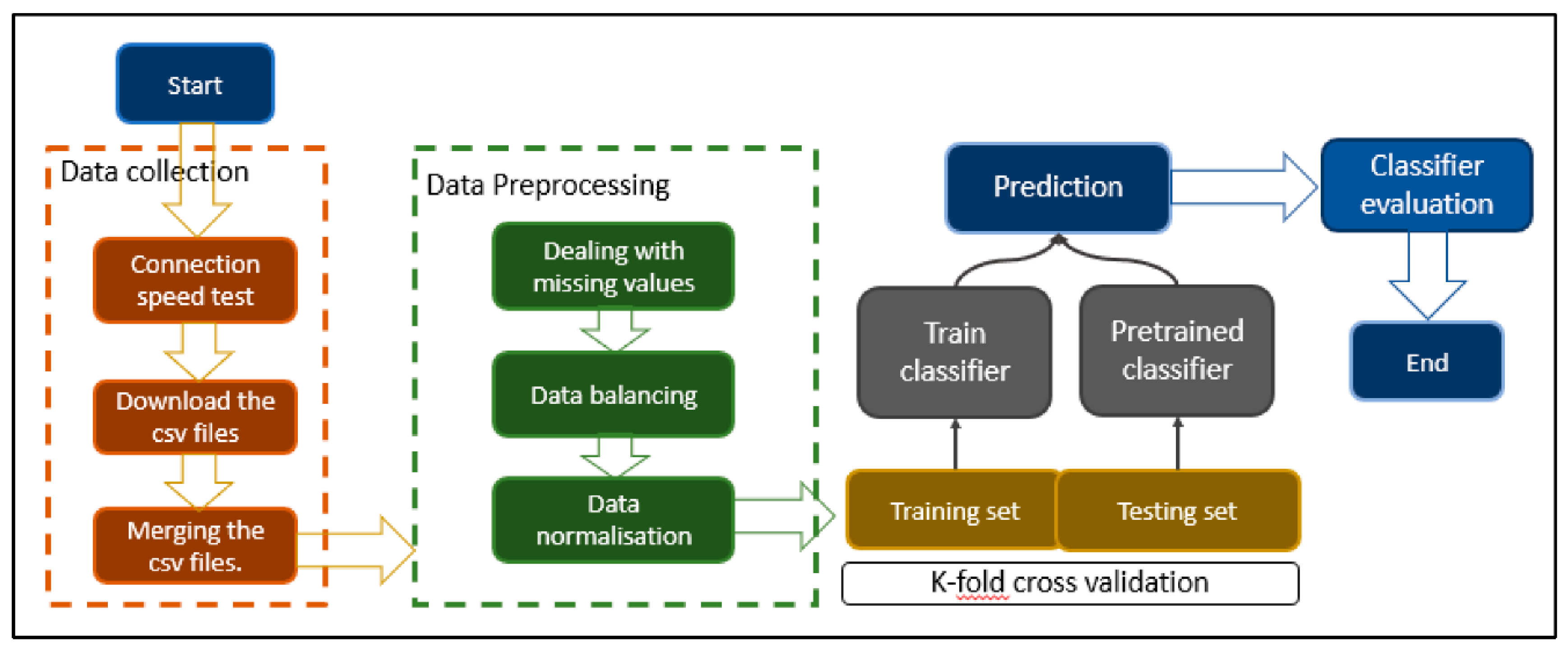
Figure 2.
The flowchart of our model.
4.1. Data Set
4.1.1. Data Collection
The connection test speed provided by the “speed.cloudflare.com” website, which enables network connectivity to be assessed from a computer connected to the network, served as the basis for the data used in this article. It enables instantaneous retrieval of the parameters’ values that affect connection quality. Several computers connecting to various networks had undergone tests. When a test is launched, it takes no more than two minutes to assess the connectivity and provide the option of downloading a csv file containing the data gathered. This procedure has been repeated on many machines linked to various networks in various locations.
Now we will go through the data description, in order to give a better comprehension of every field of the dataset. This step can be achieved as follow:
4.1.2. Data Pretreatment
Data Balancing
Datasets frequently show class imbalance in real-world classification issues, where the proportion of instances in one class is much higher than that of the other class(es). Machine learning algorithms face difficulties with unbalanced datasets because they are frequently biased in favor of the majority class, which leads to subpar performance for the minority class. The idea of data balancing and various methods for addressing class imbalance are covered in this section.
In our case, after collecting the data we were dealing with class imbalance in your dataset. This requires balancing the data for an equal distribution between classes which will lead to better performance of the model. So we have applied the Synthetic Minority Over-sampling Technique (SMOTE)[12] to balance the class distribution. The Figure 3 shows the histogram of the unbalanced data and the Figure 4 shows the histogram of the data after balancing.
Data Normalization
The standardization of the scale and distribution of input features using data normalization is a key data preparation technique. Normalization improves the efficiency of machine learning algorithms and enables more accurate and stable model training by ensuring that features have zero mean and unit variance. We provide two frequently used normalizing methods in this section: Z-score normalization and Min-Max normalization.
- Z-Score Normalization: by taking the mean away and dividing by the standard deviation, Z-score normalization, sometimes referred to as standardization, changes each feature. The following is the mathematical formula for Z-score normalization:where x stands for the original feature value, represents the feature’s mean across the training dataset, and represents its standard deviation.
- Min-Max Normalization: each feature is scaled to a specific range, usually between 0 and 1, through Min-Max normalization. The following is the Min-Max normalization mathematical equation:where x is the value of the initial feature, min(X) denotes the feature’s minimum value across the training dataset, and max(X) denotes the feature’s maximum value across the training dataset.
In machine learning, both Z-score normalization and Min-Max normalization are frequently used methods. When the data distribution is roughly Gaussian, Z-score normalization is very helpful, whereas Min-Max normalization is appropriate for features with well-defined upper and lower bounds. These normalization methods make features more comparable and lessen the effect of different scales, which enhances the efficiency of machine learning algorithms. To avoid information leakage and preserve the validity of the assessment process, normalization should be applied independently to the training set and test set.
4.1.3. Correlation Analysis
Initially, we commence by scrutinizing the dataset in order to comprehend the interconnections among these 8 characteristics. Additionally, in cases where there exists multicollinearity among variables, it can lead to the generation of irrational outcomes by the model. Hence, it becomes imperative for us to pinpoint and eliminate variables exhibiting substantial correlations. The Pearson correlation coefficient serves as an effective tool for delineating the degree of association between two variables separated by a fixed distance. In this paper, we employ this coefficient to gauge the correlations among the features, and this is visually depicted in Figure 3 through a heatmap.
The correlation matrix serves as a representation of features and serves to assess their relationships. The values within the correlation matrix range from -1 to 1. When a matrix value is in close proximity to either 1 or -1, it indicates a strong influence between the associated features. In such cases, any of these highly correlated features can be chosen independently for inclusion in the proposed algorithm. As depicted in Figure 5, it is evident that, with the exception of the “ttfb” and “latency” features, all other correlation coefficient values fall below 0.7. In essence, this means that there are no features with significant correlations. Consequently, all of these features will be included in the proposed method without requiring feature selection.
4.2. Performance Assessment Criteria for the Model
In the realm of machine learning, metrics derived from the confusion matrix are commonly employed as evaluation criteria for classification algorithms. These metrics include accuracy, precision, recall, and F1-score. In this paper, we utilize these evaluation metrics to discuss our findings and results.
4.2.1. Evaluation Metrics for Classification Derived from the Confusion Matrix
The confusion matrix serves as a common tool for assessing the predictive accuracy of a model. In Table 1, we present the confusion matrix for binary classification results. In this matrix, TP (True Positive) signifies the count of correctly predicted positive instances, FN (False Negative) indicates the count of incorrectly predicted negatives, TN (True Negative) represents the count of accurately predicted negative instances, and FP (False Positive) signifies the count of negatives erroneously predicted as positives.
Precision helps answer the following question: What proportion of positive identifications were actually correct? Accuracy can be defined as follows:
Recall
Recall helps answer the following question: What proportion of actual positive results were correctly identified? Mathematically, recall is defined as follows:
F1-Score
The F1-score (%) is a metric that represents the average of both precision and recall rates, and its value falls within the range of [0, 1]. The calculation formula is presented as follows.
4.3. Result Comparison and
In this work, we evaluated the performance of five commonly employed classifiers: XGBoost, Random Forest, SVM, Decision Tree, and K Neighbors, using the test dataset. The prediction outcomes and their associated performance metrics can be found in Table 2. To facilitate a more intuitive comparison of the methods’ performance, we have visualized the results in the form of histograms in Figure 6.
As shown in Table 2 and Figure 6 for the accuracy index, XGBoost, Rondom Forest and Deision tree obtain the best results on all models with 99.95% in test accuracy and 100% in train accuracy. Of all the models, the SVM records the lowest performance in terms of accuracy with 97.62 in test accuracy and 97.74 in train accuracy.
F1-score represent the average of precision and recall. The Table 2 and Figure 6 show that the F1-score obtained by XGBoost, Random Forest and Decision tree is the highest. It’s corresponded to 99,95 %. The F1-score of SVM and K Neighbors are 97.63% and 99,80% respectively. So, SVM has the worst performance in F1-score.
5. Conclusions
In this article we have presented a machine model that will monitor environmental change for system self -adaptation. We have made a presentation of certain related works as well as the algorithms used in the construction of the model. We then carried out an experimental analysis starting from the organizational chart of our model, including data collection, pre -treatment of data, correlation analysis, comparative analysis of the results obtained, by the different classifications algorithms, Based on the commonly used performance criteria.
References
- Choi, T.Y.; Dooley, K.J.; Rungtusanatham, M. Supply networks and complex adaptive systems: Control versus emergence. J. Oper. Manag. 2001, 19, 351–366. [Google Scholar] [CrossRef]
- Lemos, D.; et al. Software Engineering for Self-Adaptive Systems : Research Challenges in the Provision of Assurances Software Engineering for Self-adaptive Systems : Research Challenges in the Provision of Assurances. no. September, 2017.
- Oreizy, P.; et al. An architecture-based approach to self-adaptive software. IEEE Intell. Syst. Their Appl. 1999, 14, 54–62. [Google Scholar] [CrossRef]
- Rutten, E.; Marchand, N.; Simon, D.; Rutten, E.; Marchand, N.; Simon, D. Computing Feedback Control as MAPE-K loop in Autonomic Computing. 2015.
- Sousa, J.P. Software Engineering for Self-Adaptive Systems II. Lect. Notes Comput. Sci. (including Subser. Lect. Notes Artif. Intell. Lect. Notes Bioinformatics), 2013, 7475, 324–353. [Google Scholar]
- Bachir, M.A.; Jellouli, I.; Said, E.G.; Souad, A. MVC-IMASAM: Model-View-Controller inspired modeling approach for system adaptation management. Colloq. Inf. Sci. Technol. Cist 2020, 2020, 127–132. [Google Scholar]
- Cetina, C.; Giner, P.; Fons, J.; Pelechano, V. A Model-Driven Approach for Developing Self-Adaptive Pervasive Systems. 2008.
- Van Der Donckt, J.; Weyns, D.; Iftikhar, M.U.; Buttar, S.S. Effective Decision Making in Self-adaptive Systems Using Cost-Benefit Analysis at Runtime and Online Learning of Adaptation Spaces 2019, 1023.
- Wang, J.; Rao, C.; Goh, M.; Xiao, X. Risk assessment of coronary heart disease based on cloud-random forest. Artif. Intell. Rev. 2023, 56, 203–232. [Google Scholar] [CrossRef]
- Wang, Y.; Pan, Z.; Dong, J. A new two-layer nearest neighbor selection method for kNN classifier. Knowledge-Based Syst. 2022, 235, 107604. [Google Scholar] [CrossRef]
- Cao, L.; Tay, F.E.H. Financial Forecasting Using Support Vector Machines. Neural Comput. Appl. 2001, 10, 184–192. [Google Scholar] [CrossRef]
- Chawla, N.V.; Bowyer, K.W.; Hall, L.O.; Kegelmeyer, W.P. snopes.com: Two-Striped Telamonia Spider. J. Artif. Intell. Res. 2002, 16, 321–357. [Google Scholar] [CrossRef]
Figure 3.
unbalanced data histogram.
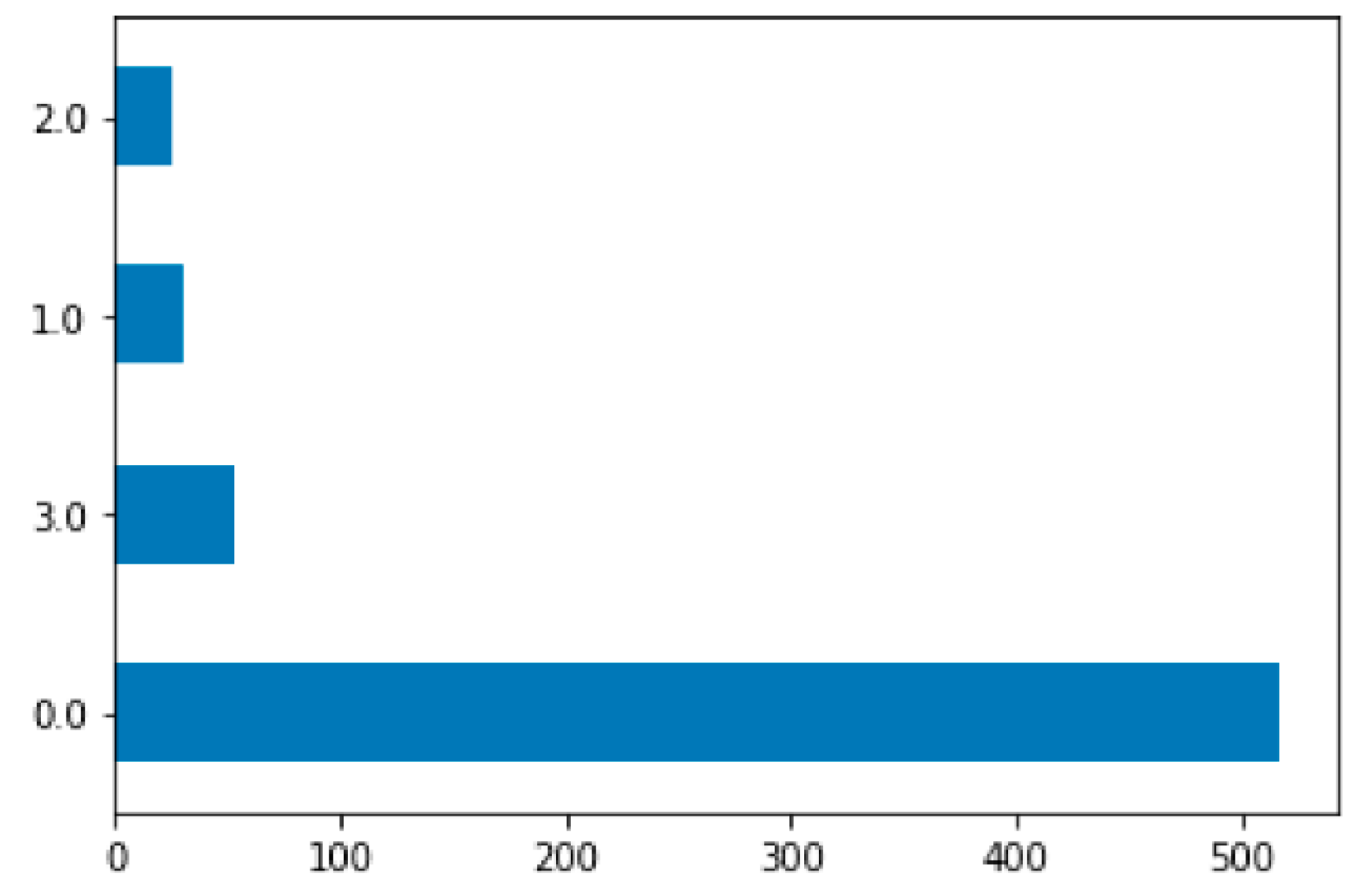
Figure 4.
balanced data histogram.
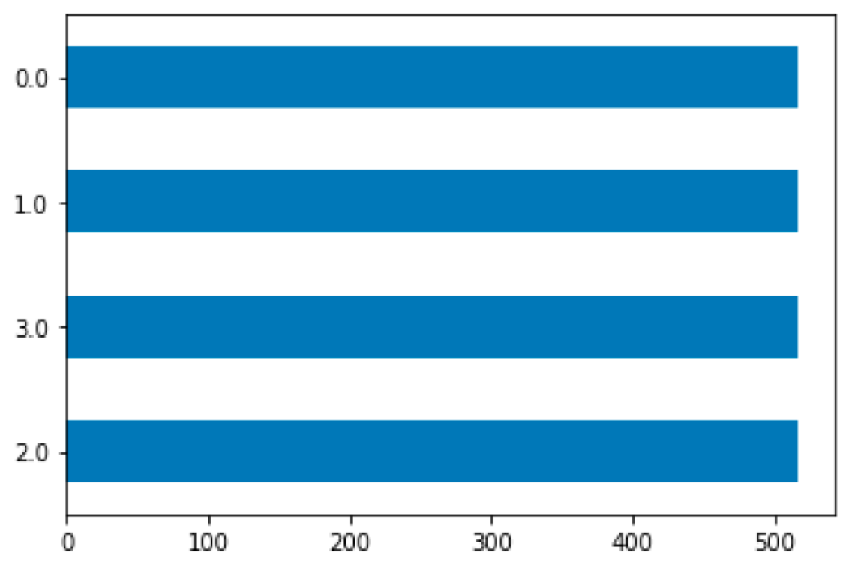
Figure 5.
Correlation matrix of the data set characteristics.

Figure 6.
The histograms of performance comparison between algorithms.
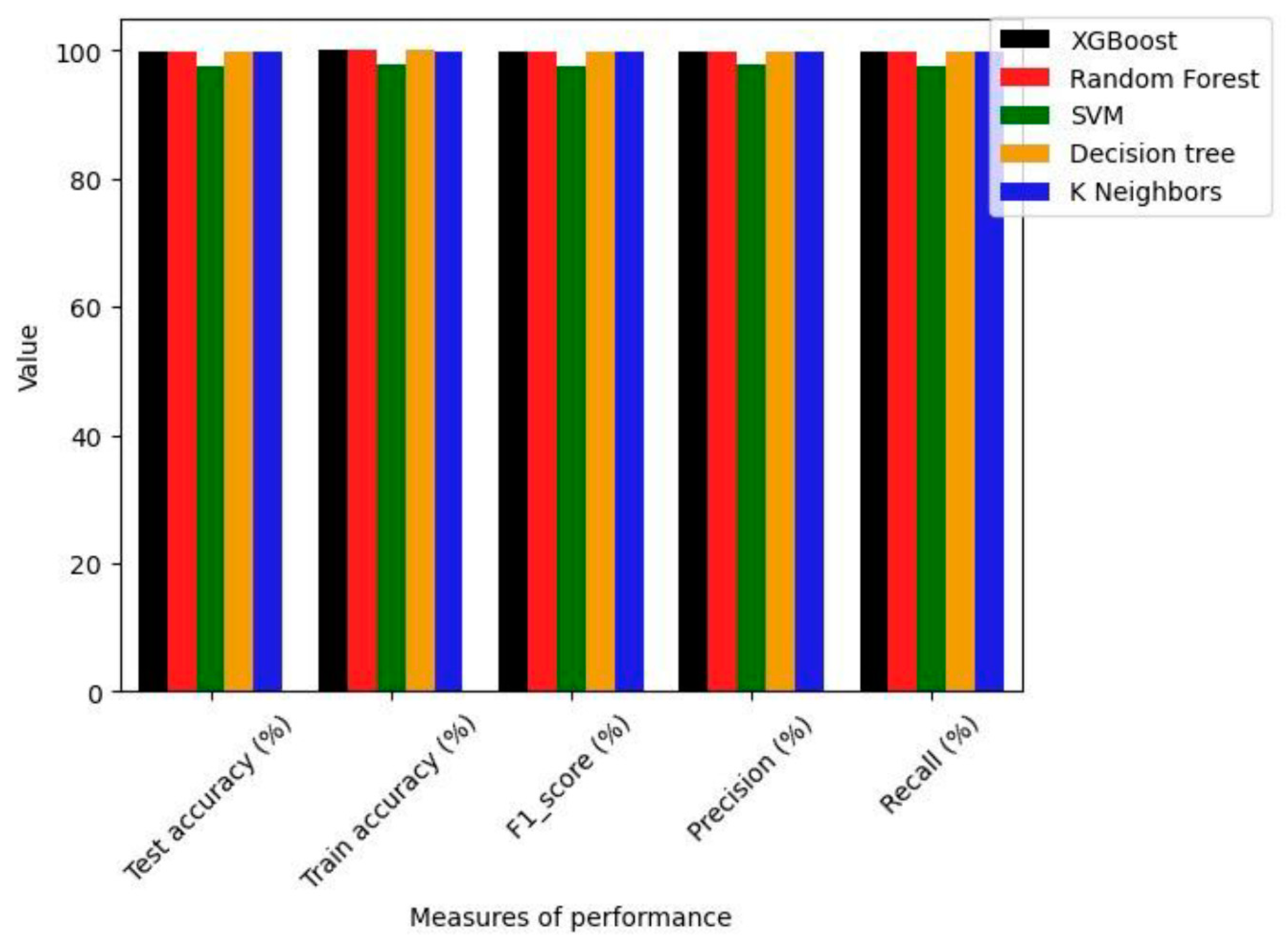

Table 1.
Data description.
| Bps | Determines the speed that the connection reach, when downloading data from a server. The others parameters are used to determine this actual value. It is tested by downloading files of various sizes. |
| Latency | Represents the time that take a piece of data to go from the computer to the server and come back. |
| TTFB | Means Time To First Byte expresses in milliseconds the time between the submission of a request to the server, and the reading of the first byte of the request, by the server. |
| Time | represents the total time to take to evaluate the connection. |
| Server Time | Represents the processing time on the server, without considering the time elapsed between the server and the computer. |
| Response Size | Represents the size of the data returned by the server in response to the request submitted by the computer. |
| Content Download Time | Determines the time taken to download the response returned by the servers. |
Table 2.
Precision.
| Predicted Positive | Predicted Negative | |
| Real Positive | TP | FN |
| Real Negative | FP | TN |
Table 3.
Prediction outcomes.
| Model | Test accuracy (%) | Train accuracy (%) | F1 score (%) | Precision (%) | Recall (%) |
| XGBoost | 99.95 | 100 | 99.95 | 99.95 | 99.95 |
| Random Forest | 99.95 | 100 | 99.95 | 99.95 | 99.95 |
| SVM | 97.62 | 97.74 | 97.63 | 97.75 | 97.62 |
| Decision tree | 99.95 | 100 | 99.95 | 99.95 | 99.95 |
| K Neighbors | 99.80 | 99.84 | 99.80 | 99.81 | 99.80 |
Disclaimer/Publisher’s Note: The statements, opinions and data contained in all publications are solely those of the individual author(s) and contributor(s) and not of MDPI and/or the editor(s). MDPI and/or the editor(s) disclaim responsibility for any injury to people or property resulting from any ideas, methods, instructions or products referred to in the content. |
© 2025 by the authors. Licensee MDPI, Basel, Switzerland. This article is an open access article distributed under the terms and conditions of the Creative Commons Attribution (CC BY) license (http://creativecommons.org/licenses/by/4.0/).
Copyright: This open access article is published under a Creative Commons CC BY 4.0 license, which permit the free download, distribution, and reuse, provided that the author and preprint are cited in any reuse.


