
Submitted:
18 April 2025
Posted:
21 April 2025
You are already at the latest version
Abstract
This study addresses the challenges of characterizing Aerosol Optical Depth (AOD) dynamics from satellite observations, which are often hindered by data gaps and variability. A Long Short-Term Memory (LSTM) network was trained on an extended AOD dataset from Sicily to capture temporal patterns. The trained model was then applied to AOD data from distinct geographical regions: Cluj-Napoca and the Central Mediterranean Sea. While the LSTM effectively captured general seasonal trends, it tended to smooth extreme AOD events. To mitigate this, a post-processing algorithm was developed to enhance the representation of AOD peaks and valleys. This enhancement method refines the characterization of historical AOD, providing a more accurate representation of observed atmospheric variability, particularly in capturing high and low AOD episodes. The results demonstrate the efficacy of the hybrid approach in improving the characterization of AOD dynamics across different regions.
Keywords:
aerosol
; AOD modelling
; MODIS
; LSTM
; peak detection
1. Introduction
Atmospheric aerosols play a crucial role in the Earth’s climate system by directly scattering and absorbing solar radiation and indirectly influencing cloud formation and properties [1,2,3]. Precise monitoring and analysis of aerosols’ spatial and temporal variations are essential because of their significant effects on climate, air quality, and public health [4,5]. Satellite remote sensing has become a vital tool for observing aerosol optical depth (AOD) across regional to global scales, providing consistent and long-term datasets that are indispensable for advancing climate and air quality research [6,7,8,9,10]. Cloud cover, acquisition methods, and temporal discontinuities frequently limit satellite-based AOD retrievals [11,12]. Continuous monitoring and forecasting could prove more challenging due to these limitations, particularly in regions where aerosol events are frequent. Advanced machine learning methods, such as LSTM networks tailored for time-series analysis, offer a promising alternative for enhancing AOD prediction accuracy by capturing complex temporal patterns and filling gaps in missing data. Furthermore, by improving the spatial resolution of AOD predictions, these innovative machine-learning algorithms can enable more thorough aerosol event monitoring. Researchers can improve the overall accuracy and dependability of AOD predictions by fusing machine-learning models with satellite-based observations.
NASA’s MODIS sensors, onboard Terra (since 2000) and Aqua (since 2002), have provided a consistent, long-term record of global aerosol observations [13]. With wide swath coverage (2330 km, ±55°), they deliver near-daily data at different times—Terra in the morning (10:30 LT) and Aqua in the afternoon (13:30 LT)—supporting diurnal aerosol studies [13]. MODIS uses 36 spectral bands across various resolutions (250 m–1 km), and retrieves AOD via three main algorithms: Dark Target (for vegetated areas and ocean), Deep Blue (for bright land), and MAIAC [13,14,15]. Unlike DT and DB, MAIAC processes time-series data over fixed grids, allowing it to better handle complex or bright surfaces through multi-angle analysis and surface BRF retrievals [15,16]. This leads to more accurate aerosol estimates, especially in challenging conditions. MAIAC has been validated globally against AERONET, with generally good agreement, though accuracy varies with factors like aerosol type, loading, and view geometry [11,12,16,17,18,19,20,21,22,23,24,25,26]. It performs well over vegetation, bright land, and during smoke events [15,16,18], making it a valuable tool for regional aerosol studies, air quality assessments, and PM estimation [20,21,27,28,29,30].
Artificial Intelligence (AI), Machine Learning (ML), and especially Deep Learning (DL) are increasingly enhancing satellite-based AOD retrieval by capturing complex, non-linear patterns beyond the reach of traditional algorithms [31,32]. Transformer-based models, such as TMAT [33] and AeroTrans-Landsat [31], directly retrieve AOD from multi-angle, multi-spectral data without heavy reliance on surface or aerosol assumptions [34]. These models also integrate meteorological inputs and underused spectral bands to boost accuracy [35,36,37]. Beyond retrieval, AI aids in post-processing existing AOD products, enabling efficient correction and reanalysis [36]. Pretrained DL models further help in data-scarce regions, extracting meaningful patterns where ground validation is limited [37].
Despite these advancements, several challenges exist in employing AI, ML, and DL for satellite AOD retrieval. One major challenge is the sensitivity of these models to fluctuations in both surface and atmospheric conditions [32]. Models trained on data from one region might face difficulties in accurately predicting AOD in new spatiotemporal domains due to substantial variations in natural conditions and the influence of anthropogenic emissions like dust and haze [32]. The availability of sufficient and accurately labelled training data remains a critical factor [38], as the performance of these data-driven models heavily relies on the quality and representativeness of the data they are trained on [39].
Satellite-derived AOD, frequently sourced from MODIS instruments at temporal resolutions ranging from daily to monthly intervals [40], represents a cornerstone dataset for understanding atmospheric composition, air quality dynamics, and climate system interactions. However, its effective utilization is often hampered by observational gaps and complex spatiotemporal variability. Addressing these challenges, Long Short-Term Memory (LSTM) neural networks have garnered significant attention, owing to their inherent architecture designed to capture long-range temporal dependencies crucial for analyzing time-series satellite observations. Their application permeates multiple facets of AOD research, starting with environmental impact analysis. LSTMs directly contribute to public health assessments by enabling the prediction of surface air pollutants strongly correlated with AOD, such as PM₂.₅ and NO₂ [39,40].
While ML use in AOD prediction is expanding, studies applying advanced models like LSTM remain relatively few. Still, recent research shows strong potential. A hybrid SARIMA-LSTM model, optimized with PSO, effectively separated linear and nonlinear AOD components in Delhi, outperforming traditional models [41]. Similarly, CNN-LSTM and ConvLSTM architectures have been used to predict dust storm dynamics using environmental data, enhancing spatial and temporal accuracy [42]. In North Bengal, MODIS AOD combined with meteorological inputs proved effective for PM₁₀ estimation via various ML models [43]. LSTM networks applied to MERRA-2 data also captured seasonal AOD patterns more accurately than conventional approaches, showing promise in data-scarce regions [44].
Building on recent findings, the present study examines the use of LSTM networks to address observational gaps and improve the temporal consistency of monthly AOD data. Under the constraint of limited satellite observations, the investigation assesses the capacity of machine learning techniques to support more reliable aerosol monitoring frameworks across three geographically distinct regions. The results indicate that LSTM models effectively capture complex temporal patterns in AOD, providing a robust method for improving aerosol observation. By employing machine learning to mitigate data limitations and refine the temporal resolution of AOD predictions, this work contributes to ongoing advancements in remote sensing and atmospheric monitoring.
2. Methodology
This study employs a machine learning approach, specifically a Long Short-Term Memory (LSTM) network combined with targeted post-processing techniques, to characterize the dynamics of Aerosol Optical Depth (AOD) derived from satellite observations. The core model was developed using an extended dataset for Sicily, and its performance in characterizing AOD dynamics was subsequently evaluated for two distinct regions: Cluj-Napoca, Romania, and the broader Central Mediterranean Sea.
The authors acknowledge that generative AI tools were utilized during this study to support various aspects of the research process. These included code optimization and debugging, exploratory data analysis guidance, and assistance in drafting and refining portions of the manuscript text. All outputs were carefully reviewed, validated, and edited by the authors to ensure scientific accuracy and originality.
2.1. Data Description and Preprocessing
2.1.1. Study Regions
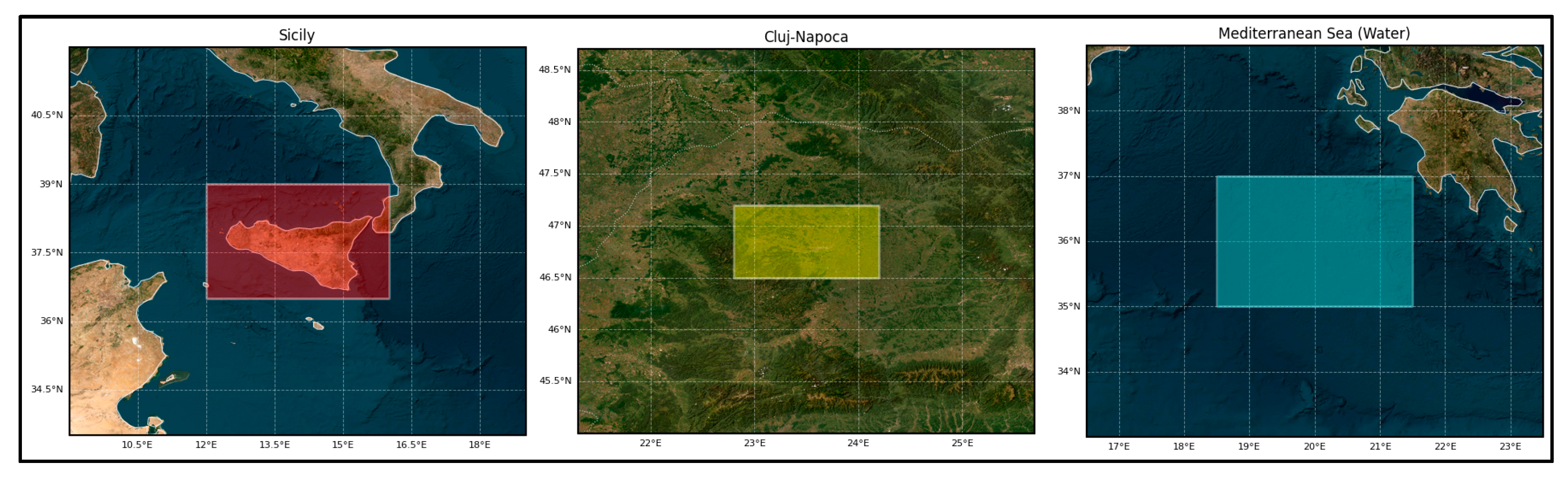
Three distinct geographical areas were central to this investigation. Firstly, Sicily, Italy, delineated by the approximate bounding box [12.0°E, 36.5°N, 16.0°E, 39.0°N], served as the primary region for initial data exploration, comprehensive model development, and subsequent training phases. This region utilized an extended historical dataset, potentially spanning 2000-2018, to ensure the model captured long-term variability and robust seasonal patterns. Secondly, Cluj-Napoca, Romania, defined by the bounding box [22.8°E, 46.5°N, 24.2°E, 47.2°N], was selected as a representative continental European urban area, presenting aerosol characteristics and meteorological conditions contrasting with the Mediterranean environment [45,46,47]. Thirdly, the Central Mediterranean Sea, encompassed within the approximate bounding box [10.0°E, 34.0°N, 20.0°E, 38.0°N], was chosen as a maritime analysis region subject to influences from sea salt aerosols, long-range atmospheric transport phenomena including Saharan dust events [48], and emissions from shipping activities.
Figure 1.
Illustration of the three study areas chosen for the model (left: Sicily, middle: Cluj-Napoca, right: Mediterranean Sea).
Figure 1.
Illustration of the three study areas chosen for the model (left: Sicily, middle: Cluj-Napoca, right: Mediterranean Sea).
2.1.2. Data Acquisition
Monthly Level 3 AOD data were procured from the Moderate Resolution Imaging Spectroradiometer (MODIS) Terra sensor, specifically utilizing the MODIS/006/MOD08_M3 product, which provides global data at a 1x1 degree spatial resolution [49]. Data acquisition and initial spatial aggregation were efficiently managed using the Google Earth Engine (GEE) platform [50]. The temporal scope of the data collection extended from January 2000 to December 2023, facilitating the analysis of long-term AOD variability and seasonality. The principal variable extracted was Aerosol_Optical_Depth_Land_Mean_Mean_550 (AOD at 550 nm). Additionally, other potentially relevant variables such as Aerosol_Optical_Depth_Land_Ocean_Mean_Mean, Deep_Blue_Aerosol_Optical_Depth_550_Land_Mean_Mean, Deep_Blue_Angstrom_Exponent_Land_Mean_Mean, Aerosol_Optical_Depth_Small_Ocean_Mean_Mean_550, and Cloud_Fraction_Mean_Mean were extracted where available. The GEE processing involved filtering the image collection by date for the specified period and subsequently calculating the monthly mean value of each variable within the defined bounding box for each study region using the ee.Image.reduceRegion() function with ee.Reducer.mean(). A spatial scale pertinent to the product resolution, such as 10000 meters, was employed for this aggregation. The resulting data, containing date stamps and corresponding mean variable values, were exported as feature collections.
2.1.3. Data Preprocessing Pipeline
The raw time series data obtained from GEE were subjected to essential preprocessing steps implemented within the pandas library environment. Initially, the extracted features were structured into a pandas DataFrame, establishing the date column as a formal datetime index for time-based operations. A critical step involved addressing missing data points (NaN values), which frequently occur in satellite-derived time series due to factors like cloud obscuration or retrieval algorithm limitations. This was handled through a sequential imputation strategy: first, linear interpolation based on the time index (interpolate(method='time')) was applied to fill gaps situated within the main body of the time series; subsequently, any remaining NaNs, typically located at the beginning or end of the series, were imputed using a forward fill followed immediately by a backward fill (fillna(method='ffill').fillna(method='bfill')). This comprehensive approach ensured the creation of a complete and temporally continuous monthly time series suitable for subsequent modeling efforts.
2.2. Feature Engineering
To augment the LSTM model’s capacity to discern and learn temporal patterns, particularly inherent seasonality, supplementary features were engineered from the datetime index. The cyclical nature of seasons was explicitly encoded through sine and cosine transformations of the month number, generating month_sin and month_cos features [51].
Additionally, a binary indicator feature, termed is_transition, was introduced to explicitly flag months identified a priori as potential transition periods between dominant seasonal atmospheric regimes [52]; in this study, February, April, June, and December were designated as such transition months, based on the patterns observed in the MODIS data, receiving a value of 1.0, while all other months were assigned 0.0. The final input feature set (X) provided to the LSTM model thus comprised the primary AOD_550 variable alongside the engineered temporal features (month_sin, month_cos, is_transition) and potentially other relevant MODIS variables selected during the development phase based on their informational content (e.g., Deep_Blue_AOD_550, Angstrom Exponent). The sole target variable (y) for the model remained the AOD_550 value at the prediction time step.
2.3. Time Series Modeling: LSTM Network
A LSTM network, recognized for its efficacy in sequence modeling and capturing complex temporal dependencies, was constructed and trained using the TensorFlow/Keras library [52,53,54].
2.3.1. Sequence Preparation
Prior to model training, the time series data underwent several preparation steps. Both the input features (X) and the target variable (y) were independently scaled to a normalized range of [0, 1] utilizing the MinMaxScaler from the sklearn.preprocessing module [55]; this scaling enhances numerical stability and convergence during training.
where:
- X is the raw feature vector.
- Xmin , Xmax are the minimum and maximum values in the dataset.
- Xnorm scales values to [0,1].
Separate scaler objects were maintained for features and the target to facilitate the accurate inverse transformation of model predictions back to the original AOD scale [55]. The continuous time series was then transformed into input-output sequences suitable for the LSTM using a sliding window methodology. Each input sequence encompassed data from the preceding 12 months (seq_length=12), and the corresponding target was the AOD value at the subsequent month.
where:
- X(t) represents the feature vector at time t.
- AOD(t−k) is the AOD value observed k months before time t.
which maps to the target variable:
where:
- Y(t) is the AOD value at the next time step to be predicted.
Finally, the dataset derived from the extended Sicily data was chronologically partitioned into training (70%), validation (15%), and testing (15%) subsets [52], ensuring that the model evaluation was performed on unseen future data relative to the training period.
2.3.2. Model Architecture
The LSTM model was implemented as a sequential Keras architecture [52,54]. The first layer consisted of an LSTM layer (LSTM) with 64 hidden units, configured to accept input sequences of shape (seq_length, num_features). This was followed by a Dropout layer with a rate of 0.2, serving as regularization to mitigate overfitting by randomly setting a fraction of input units to zero during training [56]. Dropout is a regularization technique applied during training [56]. For a layer with input activations h, Dropout with rate p=0.2 works as follows during training:
A binary mask m of the same shape as h is randomly generated, where each element mi is drawn from a Bernoulli distribution: mi∼Bernoulli(1−p). So, approximately p×100% of the elements in m will be 0, and (1−p)×100% will be 1 [56].
- The output h′ is calculated by element-wise multiplication:
To compensate for the dropped units and keep the expected sum of activations the same, the output is scaled by 1/(1−p) (this is often done automatically by implementations):
Subsequently, a fully connected Dense layer with 32 units and a Rectified Linear Unit (relu) activation function was included to introduce further non-linearity [57,58]. The final layer was a single Dense unit with a linear activation function, outputting the predicted scaled AOD_550 value. This is a fully connected standard layer. Which takes an input vector , where = 64, and produces an output vector . The linear activation function:
Where , is the weight matrix and is the bias vector. The rectified linear unit activation function is applied elementwise:
Thus,
The final Dense layer takes the output of the previous Dense layer and produces the final single prediction , performing the linear transformation:
Where w is the weight vector (technically in the form of a 1 x 32 matrix) and b is the scalar bias. No activation function is applied.
The LSTM model follows the standard formulation of input gate, forget gate, cell state update, output gate and hidden state, detailed in [52].
2.3.3. Training Procedure
The model was compiled and trained using the Adam optimizer (tf.keras.optimizers.Adam) initialized with a learning rate of 0.001 [59]. Mean Squared Error (MSE) was selected as the loss function [60], quantifying the average squared difference between predicted and actual scaled AOD values. Two key callbacks were employed during training to manage the learning process and enhance generalization. An EarlyStopping callback monitored the validation loss (val_loss) and terminated training if no improvement was observed for 20 consecutive epochs, automatically restoring the model weights corresponding to the epoch with the lowest validation loss [61]. Concurrently, a ReduceLROnPlateau callback monitored the same validation loss metric and reduced the learning rate by a factor of 0.5 if it plateaued for 10 epochs, with a predefined minimum learning rate threshold of 0.0001 [60]. The model training was executed on the prepared extended Sicily dataset for a maximum duration of 150 epochs, utilizing a batch size of 16.
2.4. Application to Analysis Regions
Following successful training and validation on the Sicily dataset, the resulting trained LSTM model, embodying the learned AOD dynamics, was applied to the preprocessed, scaled, and sequence-formatted datasets corresponding to the Cluj-Napoca and Central Mediterranean Sea regions. This application generated the baseline AOD predictions (y_pred_orig after inverse scaling) for these distinct analysis areas, serving as the input for the subsequent post-processing enhancement steps.
2.5. Post-Processing and Analysis
Recognizing that standard LSTM predictions can sometimes attenuate the amplitude of sharp peaks and valleys in time series data [62], dedicated post-processing steps were designed and applied independently to the test set predictions for each study region. These steps aimed to refine the characterization of these critical high- and low-AOD events.
2.5.1. Temporal Alignment
To address potential phase discrepancies between the predicted AOD variations and the observed data, a temporal alignment procedure was implemented [63]. Cross-correlation was computed between the actual AOD test data (y_test_orig) and the inverse-scaled baseline LSTM predictions (y_pred_orig) using the scipy.signal.correlate function [64]. The temporal lag corresponding to the maximum value in the resulting cross-correlation function was identified. The entire predicted time series (y_pred_orig) was then shifted (advanced or delayed) by this optimal lag, yielding a temporally aligned prediction series (y_aligned_orig). This alignment ensures that the timing of predicted features corresponds optimally with the ground truth before applying magnitude adjustments.
2.5.2. Peak and Valley Enhancement
A custom algorithm, termed enhanced_peak_valley_amplification, was developed to specifically enhance the representation of significant extrema (peaks and valleys) in the AOD signal. Initially, prominent peaks and valleys within the actual AOD test data (y_test_orig) were detected using the scipy.signal.find_peaks function. Peaks were identified directly, while valleys were located by applying the same function to the inverted signal (-y_test_orig). A prominence threshold of 0.04 was employed to filter for physically significant extrema, excluding minor fluctuations.
Let be the actual observed AOD at time index t. is the aligned base LSTM prediction at time index t, and p is the peak detected at in with proeminence 0.04. For each detected actual extremum occurring at index i, a multi-step enhancement was applied to the corresponding value in the temporally aligned prediction (y_aligned_orig[i]). First, the predicted value was adjusted by moving it 60% of the way from its current level towards the actual extremum’s magnitude (y_test_orig[i]).
Second, the prominence of this 60%-adjusted value relative to its immediate neighbors in the predicted series was calculated. An initial base level was determined:
Consequently, the prominence level was calculated:
Then, the prominence was amplified with the amplification factor :
Next, the prominence-amplified height was determined:
Lastly, the final enhanced value for the peak was set:
Third, this calculated prominence was amplified by a factor of 1.2 (amplification_factor). The final enhanced value (y_enhanced_orig[i]) was then determined by selecting the maximum (for peaks) or minimum (for valleys) between the 60%-adjusted value and the prominence-amplified value, ensuring the enhancement captured both magnitude correction and relative significance.
To ensure smooth transitions around these enhanced points, a localized smoothing mechanism was applied within a small window (window_size=2) adjacent to each enhanced extremum. Neighboring points within this window were adjusted by a fraction (0.3) of the enhancement magnitude applied at the extremum, with the adjustment weighted by proximity.
Where, w(k) is a weighted factor decreasing with distance k and fsmooth is the smoothing factor.
Furthermore, a subtle “Transition Month Boost” was incorporated: values within the enhanced series (y_enhanced_orig) that corresponded to the predefined transition months (February, April, June, December) were multiplied by a factor of 1.03. The justification for this comprehensive enhancement procedure lies in its objective to produce a final time series (y_enhanced_orig) that more accurately reflects the observed magnitude and sharpness of AOD peaks and valleys, thereby providing a richer characterization of the atmospheric system’s dynamics than the potentially smoothed baseline LSTM output, while using conservative amplification factors to avoid excessive distortion.
2.6. Evaluation Metrics and Statistical Analysis
The performance of the modeling framework was quantitatively assessed using standard error metrics, namely Root Mean Squared Error (RMSE) and Mean Absolute Error (MAE). These metrics were calculated to compare the actual AOD observations (y_test_orig) against the predictions at various stages: the baseline LSTM output (y_pred_orig), the temporally aligned predictions (y_aligned_orig), and the final enhanced predictions (y_enhanced_orig). The evaluations were conducted across the entire test set for each region, and specifically focused on the identified peak and valley locations to gauge the effectiveness of the enhancement procedure on extrema. Beyond error metrics, further statistical analysis was performed on the characteristics of the identified peaks and valleys. This included analyzing their seasonal distribution to understand typical periods of high and low AOD occurrence within each region. Additionally, the average time difference between identified peaks and their nearest subsequent valleys was calculated, providing insight into the characteristic duration of elevated AOD events.
3. Results
This study employed a hybrid methodology, integrating a LSTM network with signal processing and targeted adjustments, aimed at the detailed characterization rather than prediction of historical AOD dynamics. The LSTM model, trained on an extensive dataset capturing over two decades of AOD variability in Sicily, served as the foundation for capturing underlying seasonal patterns and trends.
3.1. Model Performance in the Training Region
The LSTM model was initially trained using an extended historical AOD dataset for Sicily. Its performance was evaluated on a withheld portion of this dataset corresponding to the period (2015-2017). The results are visually presented in Figure 2.
The temporally aligned base LSTM prediction (red dashed line) successfully captured the overall seasonal AOD cycle characteristic of Sicily, achieving an overall RMSE of 0.0591 and MAE of 0.0462 against the observed MODIS AOD (blue line). However, Figure 2 also clearly illustrates the model’s tendency to smooth extreme events; the magnitudes of observed peaks (green triangles) are frequently underestimated, while the depths of observed valleys (red triangles) are overestimated by the base prediction. This limitation is reflected in the higher error metrics calculated specifically for these extrema (Peak RMSE: 0.0690, MAE: 0.0595).

Table 1.
Error Metrics for Training & Test Set (Sicily).
| Model | Metric | Value |
|---|---|---|
| Base | Overall RMSE | 0.0591 |
| Base | Overall MAE | 0.0462 |
| Enhanced | Overall RMSE | 0.0494 |
| Enhanced | Overall MAE | 0.0279 |
| Base | Peak RMSE | 0.0690 |
| Base | Peak MAE | 0.0595 |
| Enhanced | Peak RMSE | 0.0192 |
| Enhanced | Peak MAE | 0.0131 |
To address this representation gap, the enhanced_peak_valley_amplification post-processing step was applied. This algorithm uses the observed peaks and valleys from the test period to adjust the aligned prediction, aiming for a more accurate characterization of historical variability. The resulting enhanced prediction (solid green line in Figure 2) demonstrates a markedly improved agreement with the observed AOD during peak and valley occurrences. This visual improvement is corroborated by substantial reductions in the extrema-specific error metrics (Enhanced Peak RMSE: 0.0192, Enhanced Peak MAE: 0.0131), while the overall error remained comparable (Enhanced Overall RMSE: 0.0494). This confirms the effectiveness of the enhancement procedure in correcting the base model’s smoothing specifically at points of high AOD variability within the training region’s test set.
3.2. Model Generalization: Case Studies
To assess the applicability and limitations of the Sicily-trained model and the enhancement methodology in different environments, the trained LSTM was applied without modification to AOD time series from two distinct regions.
3.2.1. Cluj-Napoca (Continental Land Region)
The Sicily-trained LSTM model was applied to the 2000-2018 MODIS AOD dataset for Cluj-Napoca, Romania. The results, focusing on the long-term comparison of model outputs and actual data, are shown in Figure 3. The base LSTM prediction (red dashed line) exhibits an attempt to follow the seasonal pattern observed in Cluj, achieving an overall RMSE of 0.0587 and MAE of 0.0444.
However, visual inspection of Figure 3 reveals that the model, tuned to Sicilian dynamics, struggles to capture the sharper, higher-amplitude peaks often observed during Cluj summers. Applying the enhancement algorithm, using Cluj’s local ground-truth extrema for adjustment, yielded the enhanced prediction (green line). This enhanced curve provides a significantly better representation of the observed peak magnitudes, reflected in improved peak-specific metrics (Enhanced Peak RMSE: 0.0215), and offers a more accurate overall historical characterization (Enhanced Overall RMSE: 0.0459). Figure 3 highlights the distinct AOD regime in Cluj compared to Sicily, characterized by potentially higher intra-annual variability and stronger peak events.
Table 2.
Error Metrics for Case Study on Continental Region (Cluj-Napoca).
| Model | Metric | Value |
|---|---|---|
| Base | Overall RMSE | 0.0587 |
| Base | Overall MAE | 0.0444 |
| Enhanced | Overall RMSE | 0.0459 |
| Enhanced | Overall MAE | 0.0342 |
| Base | Peak RMSE | 0.0784 |
| Base | Peak MAE | 0.0596 |
| Enhanced | Peak RMSE | 0.0215 |
| Enhanced | Peak MAE | 0.0164 |
3.2.2. Mediterranean Sea (Water Region)
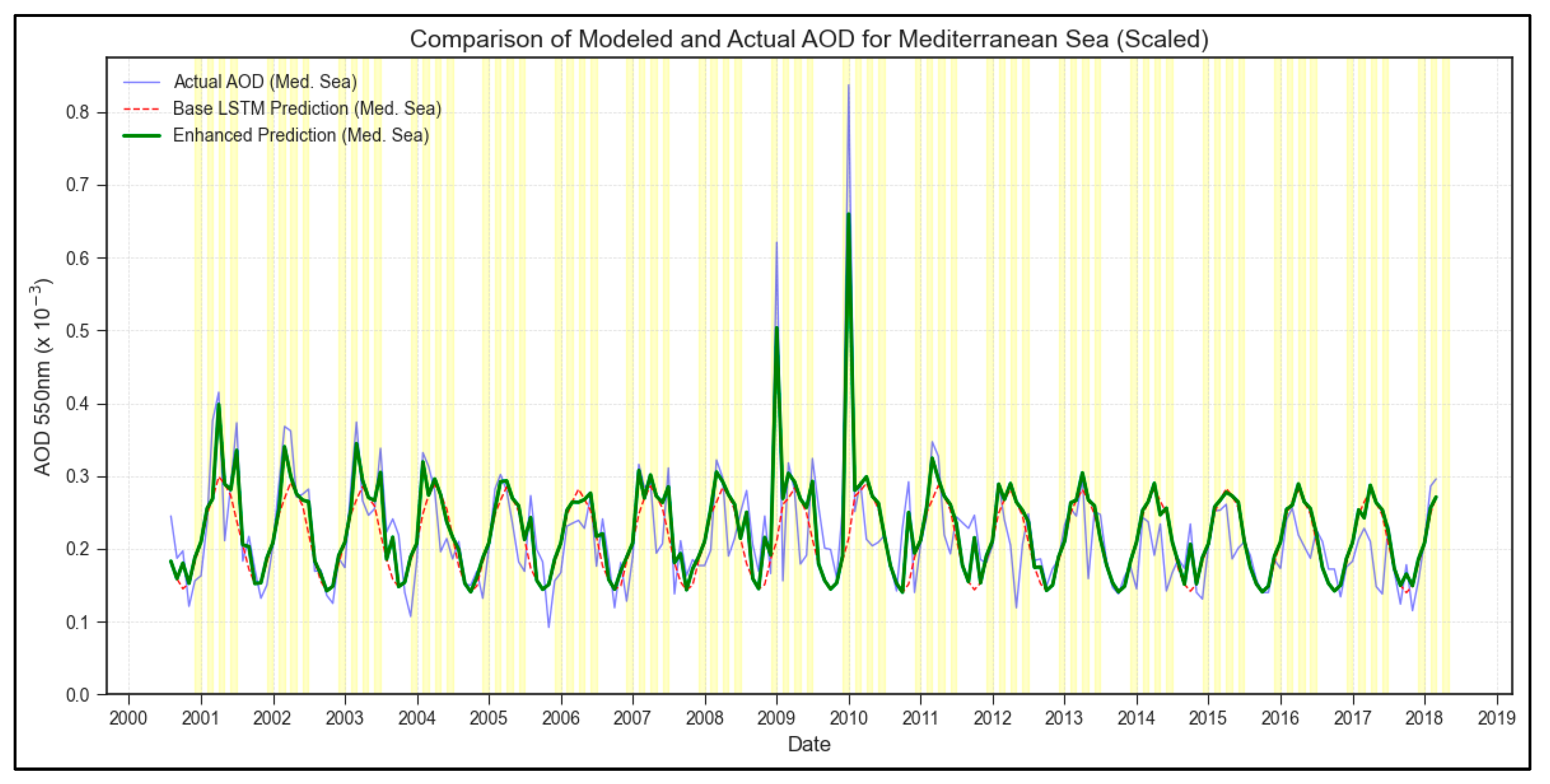
The model’s generalization was further tested over a water-only region in the Central Mediterranean Sea for the 2000-2018 period (Figure 4).
This region presents a different challenge, characterized by a relatively low baseline AOD punctuated by extreme, short-duration peaks likely associated with Saharan dust transport. The Sicily-trained base LSTM (red dashed line) captures the low baseline reasonably well but, as evident in Figure 4, fails dramatically to represent the magnitude of the major observed peaks (Overall RMSE: 0.0740). The enhancement procedure, leveraging the observed water-region extrema, effectively scales these peaks (green line), leading to a visually striking improvement in representation and a substantial reduction in peak-specific errors (Enhanced Peak RMSE: 0.0317; Enhanced Overall RMSE: 0.0536). This case study particularly emphasizes the utility of the enhancement step for characterizing episodic, extreme events that a standard model, trained in a different domain, might otherwise completely miss.
Table 3.
Error Metrics for Case Study over Water Region (Mediterranean Sea).
| Model | Metric | Value |
|---|---|---|
| Base | Overall RMSE | 0.0740 |
| Base | Overall MAE | 0.0498 |
| Enhanced | Overall RMSE | 0.0536 |
| Enhanced | Overall MAE | 0.0405 |
| Base | Peak RMSE | 0.1061 |
| Base | Peak MAE | 0.0585 |
| Enhanced | Peak RMSE | 0.0317 |
| Enhanced | Peak MAE | 0.0195 |
4. Discussion
The results demonstrate the capabilities and limitations of using an LSTM model trained on regional data for characterizing AOD dynamics and highlight the specific value of the proposed enhancement methodology. The base LSTM, trained on extended Sicilian data, proved effective at learning the dominant seasonal patterns within its training domain (Figure 2). However, its performance degraded when applied to regions with distinct climatologies and aerosol sources, namely continental Cluj-Napoca (Figure 3) and the maritime Mediterranean (Figure 4), underscoring the strong regional dependence of AOD dynamics and the challenge of model generalization. The base model consistently smoothed high-amplitude peaks and valleys across all regions, a key limitation quantified by the difference between base predictions and observed extrema.
The primary contribution of this work lies in the application and interpretation of the enhanced_peak_valley_amplification post-processing step. While this step incorporates ground-truth information from the period under analysis, rendering it unsuitable for forecasting evaluation, it provides significant value for historical characterization and analysis. Firstly, it serves as a powerful diagnostic tool, quantifying the precise magnitude and timing of the base LSTM’s underestimation of extreme events. Comparing the base and enhanced curves (e.g., in Figure 2 and Figure 4) directly visualizes the model’s structural limitations in representing phenomena like dust outbreaks or intense pollution episodes. This diagnostic insight is critical for understanding the applicability domains of standard time series models for variables exhibiting such intermittent extremes.
Secondly, the methodology yields an enhanced historical representation (y_enhanced_orig) optimized for subsequent scientific analysis. This hybrid signal merges the model’s learned seasonal baseline with accurately scaled historical peak and valley magnitudes. This product is arguably more valuable than either the noisy raw data or the smoothed base prediction for specific research goals, such as correlating the timing and intensity of accurately represented historical AOD peaks with meteorological drivers, air mass origins, or health impact assessments. The enhancement effectively creates an analysis-ready dataset where key events are represented with higher fidelity. The successful application of this enhancement across diverse regions (Land, Water and Mixed) demonstrates its robustness as a technique for improving the representation of local extremes, irrespective of the base model’s generalization performance.
Comparing the three regions reveals distinct AOD climatologies. Sicily exhibits a Mediterranean pattern with mixed influences. Cluj-Napoca shows stronger seasonality and higher variability typical of a continental site. The Mediterranean Sea displays a lower baseline dominated by extreme episodic events. The model and enhancement procedure effectively captured these differing characteristics, particularly in the enhanced representations.
4.1. Limitations
The study acknowledges limitations, primarily the use of monthly data which averages out finer temporal details, and the non-predictive nature of the enhancement method. Future work could explore higher temporal resolution data, incorporate meteorological predictors into the LSTM to improve its intrinsic generalization capabilities, investigate more complex deep learning architectures, or perform detailed source attribution for the identified peaks using trajectory models informed by the enhanced AOD time series. Developing true forecasting models that leverage the seasonal and transitional insights gained from this characterization remains a key objective.
5. Conclusions and Future Directions
5.1. Conclusions
This investigation centered on characterizing AOD dynamics utilizing a LSTM network, augmented by a bespoke post-processing methodology. The LSTM model, initially trained on a comprehensive dataset from Sicily spanning over two decades, demonstrated proficiency in capturing the underlying seasonality and general trends inherent within its training domain. However, a notable observation was the model’s inherent tendency to attenuate the magnitude of extreme AOD events, namely sharp peaks and deep valleys, a limitation consistently observed across all test regions.
The application of the trained model to distinct geographical areas – continental Cluj-Napoca and the maritime Central Mediterranean – underscored the challenge of model generalization. Performance naturally varied when confronting AOD regimes differing significantly from the training environment, highlighting the strong regional specificity of aerosol behaviors.
Crucially, the introduced enhanced_peak_valley_amplification post-processing step proved highly effective. While acknowledging its reliance on ground-truth data from the analysis period (rendering it unsuitable for direct forecasting), its utility is twofold. Firstly, it functions as a potent diagnostic tool, precisely quantifying the extent to which the baseline LSTM underestimates or misrepresents extreme AOD occurrences. This offers valuable insight into the structural limitations of standard sequence models when applied to time series marked by intermittent, high-amplitude events. Secondly, and perhaps more significantly for subsequent research, the methodology yields an enhanced historical AOD representation. This refined dataset, effectively merging the model’s grasp of seasonal patterns with accurately scaled historical extrema, presents a more robust basis for specific analytical goals, such as investigating the drivers behind significant aerosol events or assessing their impacts, compared to either the raw, potentially noisy observations or the smoothed baseline model output. The procedure demonstrated robustness across diverse land, mixed, and water regions.
In essence, the combined approach provides a valuable framework not just for modeling AOD, but for critically evaluating model performance concerning extreme events and generating an analysis-ready historical dataset that more faithfully represents observed atmospheric variability, particularly during high and low AOD episodes.
5.2. Future Work and Directions
Despite the insights gained, certain limitations point toward avenues for future investigation. The reliance on monthly aggregated AOD data inevitably obscures finer temporal details; exploring the application of similar methodologies to higher-resolution datasets (e.g., daily) could reveal sub-monthly dynamics currently averaged out.
To improve the intrinsic predictive power and generalization capabilities of the core model, future iterations could benefit substantially from the incorporation of relevant meteorological predictors (e.g., wind patterns, humidity, boundary layer height) directly into the LSTM architecture. This might allow the model to learn more complex relationships driving AOD variations beyond simple seasonality.
Furthermore, investigating more sophisticated deep learning architectures, potentially hybrid models combining convolutional layers (for spatial context, if applicable) with LSTMs or employing attention mechanisms, could potentially enhance the model’s ability to capture sharp transitions and extreme events without extensive post-processing.
The enhanced AOD time series generated herein, with its accurately represented peaks, offers a prime opportunity for subsequent analysis. Coupling this data with atmospheric back-trajectory models could facilitate more detailed source attribution studies, pinpointing the origins and transport pathways associated with the identified high-AOD events.
Finally, while this study focused on historical characterization, a key objective remains the development of genuine AOD forecasting systems. Leveraging the understanding of seasonal patterns, transition periods, and the nature of extreme events gained from this work could inform the design of more accurate and reliable predictive models for future AOD conditions.
Author Contributions
Conceptualization, Horia-Alexandru Cămărășan and Nicolae Ajtai; Formal analysis, Horia-Alexandru Cămărășan and Lucia-Timea Deaconu; Funding acquisition, Nicolae Ajtai; Methodology, Horia-Alexandru Cămărășan, Alexandru Mereuță and Zoltàn Török; Supervision, Nicolae Ajtai; Validation, Horațiu-Ioan Ștefănie and Andrei-Titus Radovici; Visualization, Andrei-Titus Radovici; Writing – original draft, Horia-Alexandru Cămărășan and Camelia Botezan; Writing – review & editing, Alexandru Mereuță, Horațiu-Ioan Ștefănie and Camelia Botezan. All authors have read and agreed to the published version of the manuscript.”
Funding
The work was financed by Smart Growth, Digitization and Financial Instruments Program (PoCIDIF) 2021-2027, Action 1.3 Integration of the national RDI ecosystem in the European and international Research Space, project “Supporting the operation of facilities in Romania within the ACTRIS ERIC research infrastructure”, SMIS code 309113, ctr. no. G 2024-96579/17.12.2024/390010/19.12.2024.
Data Availability Statement
The Aerosol Optical Depth (AOD) data used in this study were sourced from the MODIS (Moderate Resolution Imaging Spectroradiometer) instrument aboard NASA’s Terra satellite. Specifically, we utilized the MODIS/Terra Gridded Level 3 Monthly Global Atmosphere Product (MOD08_M3) Version 6, obtained via Google Earth Engine. We acknowledge NASA and the MODIS Science Team for providing this data.
Acknowledgments
The authors wish to acknowledge the computational resources and software libraries that were instrumental in conducting this research. The analysis was performed using the Python programming language (v3.11) [https://www.python.org/]. We utilized several key open-source Python libraries, including:
- NumPy [https://numpy.org/] for fundamental numerical computations.
- Pandas [https://pandas.pydata.org/] for data manipulation and analysis.
- TensorFlow [https://www.tensorflow.org/] (with its Keras API) for building and training the LSTM neural network models.
- Scikit-learn [https://scikit-learn.org/] for data preprocessing tasks, particularly data scaling (MinMaxScaler).
- SciPy [https://scipy.org/] for scientific and technical computing, specifically for signal processing functions (signal.find_peaks, signal.correlate).
- Matplotlib [https://matplotlib.org/] for generating plots and visualizations.
- Google Earth Engine Python API [https://developers.google.com/earth-engine/guides/python_install] for satellite data access and initial processing.
We gratefully acknowledge the use of the Google Earth Engine platform for accessing and processing satellite imagery).
Conflicts of Interest
The authors declare no conflicts of interest.
References
- Costantino, L.; Bréon, F.-M. Aerosol Indirect Effect on Warm Clouds over South-East Atlantic, from Co-Located MODIS and CALIPSO Observations. Atmospheric Chem. Phys. 2013, 13, 69–88. [Google Scholar] [CrossRef]
- Ghan, S.J. Technical Note: Estimating Aerosol Effects on Cloud Radiative Forcing. Atmospheric Chem. Phys. 2013, 13, 9971–9974. [Google Scholar] [CrossRef]
- Carslaw, K. Aerosols and Climate; Elsevier: Amsterdam, 2022; ISBN 978-0-12-819766-0. [Google Scholar]
- Manavi, S.E.I.; Aktypis, A.; Siouti, E.; Skyllakou, K.; Myriokefalitakis, S.; Kanakidou, M.; Pandis, S.N. Atmospheric Aerosol Spatial Variability: Impacts on Air Quality and Climate Change. One Earth 2025, 8, 101237. [Google Scholar] [CrossRef]
- Oh, H.-J.; Ma, Y.; Kim, J. Human Inhalation Exposure to Aerosol and Health Effect: Aerosol Monitoring and Modelling Regional Deposited Doses. Int. J. Environ. Res. Public. Health 2020, 17, 1923. [Google Scholar] [CrossRef]
- Salomonson, V.V.; Barnes, W.L.; Maymon, P.W.; Montgomery, H.E.; Ostrow, H. MODIS: Advanced Facility Instrument for Studies of the Earth as a System. IEEE Trans. Geosci. Remote Sens. 1989, 27, 145–153. [Google Scholar] [CrossRef]
- Winker, D.M.; Vaughan, M.A.; Omar, A.; Hu, Y.; Powell, K.A.; Liu, Z.; Hunt, W.H.; Young, S.A. Overview of the CALIPSO Mission and CALIOP Data Processing Algorithms. J. Atmospheric Ocean. Technol. 2009, 26, 2310–2323. [Google Scholar] [CrossRef]
- Diner, D.J.; Beckert, J.C.; Reilly, T.H.; Bruegge, C.J.; Conel, J.E.; Kahn, R.A.; Martonchik, J.V.; Ackerman, T.P.; Davies, R.; Gerstl, S.A. Multi-Angle Imaging SpectroRadiometer (MISR) Instrument Description and Experiment Overview. IEEE Trans. Geosci. Remote Sens. 1998, 36, 1072–1087. [Google Scholar] [CrossRef]
- Deschamps, P.-Y.; Breon, F.-M.; Leroy, M.; Podaire, A.; Bricaud, A.; Buriez, J.-C.; Seze, G. The POLDER Mission: Instrument Characteristics and Scientific Objectives. IEEE Trans. Geosci. Remote Sens. 1994, 32, 598–615. [Google Scholar] [CrossRef]
- Levelt, P.F.; Van Den Oord, G.H.J.; Dobber, M.R.; Malkki, A.; Huib, Visser; Johan De, Vries; Stammes, P.; Lundell, J.O.V.; Saari, H. The Ozone Monitoring Instrument. IEEE Trans. Geosci. Remote Sens. 2006, 44, 1093–1101. [Google Scholar] [CrossRef]
- Mhawish, A.; Banerjee, T.; Sorek-Hamer, M.; Lyapustin, A.; Broday, D.M.; Chatfield, R. Comparison and Evaluation of MODIS Multi-Angle Implementation of Atmospheric Correction (MAIAC) Aerosol Product over South Asia. Remote Sens. Environ. 2019, 224, 12–28. [Google Scholar] [CrossRef]
- Tao, M.; Wang, J.; Li, R.; Wang, L.; Wang, L.; Wang, Z.; Tao, J.; Che, H.; Chen, L. Performance of MODIS High-Resolution MAIAC Aerosol Algorithm in China: Characterization and Limitation. Atmos. Environ. 2019, 213, 159–169. [Google Scholar] [CrossRef]
- Levy, R.C.; Mattoo, S.; Munchak, L.A.; Remer, L.A.; Sayer, A.M.; Patadia, F.; Hsu, N.C. The Collection 6 MODIS Aerosol Products over Land and Ocean. Atmospheric Meas. Tech. 2013, 6, 2989–3034. [Google Scholar] [CrossRef]
- Hsu, N.C.; Jeong, M.-J.; Bettenhausen, C.; Sayer, A.M.; Hansell, R.; Seftor, C.S.; Huang, J.; Tsay, S.-C. Enhanced Deep Blue Aerosol Retrieval Algorithm: The Second Generation: ENHANCED DEEP BLUE AEROSOL RETRIEVAL. J. Geophys. Res. Atmospheres 2013, 118, 9296–9315. [Google Scholar] [CrossRef]
- Lyapustin, A.; Wang, Y.; Korkin, S.; Huang, D. MODIS Collection 6 MAIAC Algorithm. Atmospheric Meas. Tech. 2018, 11, 5741–5765. [Google Scholar] [CrossRef]
- Superczynski, S.D.; Kondragunta, S.; Lyapustin, A.I. Evaluation of the Multi-angle Implementation of Atmospheric Correction (MAIAC) Aerosol Algorithm through Intercomparison with VIIRS Aerosol Products and AERONET. J. Geophys. Res. Atmospheres 2017, 122, 3005–3022. [Google Scholar] [CrossRef]
- Jethva, H.; Torres, O.; Yoshida, Y. Accuracy Assessment of MODIS Land Aerosol Optical Thickness Algorithms Using AERONET Measurements over North America. Atmospheric Meas. Tech. 2019, 12, 4291–4307. [Google Scholar] [CrossRef]
- Martins, V.S.; Lyapustin, A.; De Carvalho, L.A.S.; Barbosa, C.C.F.; Novo, E.M.L.M. Validation of High-resolution MAIAC Aerosol Product over South America. J. Geophys. Res. Atmospheres 2017, 122, 7537–7559. [Google Scholar] [CrossRef]
- Arvani, B.; Pierce, R.B.; Lyapustin, A.I.; Wang, Y.; Ghermandi, G.; Teggi, S. Seasonal Monitoring and Estimation of Regional Aerosol Distribution over Po Valley, Northern Italy, Using a High-Resolution MAIAC Product. Atmos. Environ. 2016, 141, 106–121. [Google Scholar] [CrossRef]
- Zhdanova, E.Y.; Chubarova, N.Y.; Lyapustin, A.I. Assessment of Urban Aerosol Pollution over the Moscow Megacity by the MAIAC Aerosol Product. Atmospheric Meas. Tech. 2020, 13, 877–891. [Google Scholar] [CrossRef]
- Shaylor, M.; Brindley, H.; Sellar, A. An Evaluation of Two Decades of Aerosol Optical Depth Retrievals from MODIS over Australia. Remote Sens. 2022, 14, 2664. [Google Scholar] [CrossRef]
- Zhang, Z.; Wu, W.; Fan, M.; Wei, J.; Tan, Y.; Wang, Q. Evaluation of MAIAC Aerosol Retrievals over China. Atmos. Environ. 2019, 202, 8–16. [Google Scholar] [CrossRef]
- Qin, W.; Fang, H.; Wang, L.; Wei, J.; Zhang, M.; Su, X.; Bilal, M.; Liang, X. MODIS High-Resolution MAIAC Aerosol Product: Global Validation and Analysis. Atmos. Environ. 2021, 264, 118684. [Google Scholar] [CrossRef]
- Lee, S.; Pinhas, A.; Alexandra, C.A. Aerosol Pattern Changes over the Dead Sea from West to East - Using High-Resolution Satellite Data. Atmos. Environ. 2020, 243, 117737. [Google Scholar] [CrossRef]
- Emili, E.; Lyapustin, A.; Wang, Y.; Popp, C.; Korkin, S.; Zebisch, M.; Wunderle, S.; Petitta, M. High Spatial Resolution Aerosol Retrieval with MAIAC: Application to Mountain Regions: HIGH SPATIAL RESOLUTION AEROSOL RETRIEVAL. J. Geophys. Res. Atmospheres 2011, 116, n/a-n/a. [Google Scholar] [CrossRef]
- Falah, S.; Mhawish, A.; Sorek-Hamer, M.; Lyapustin, A.I.; Kloog, I.; Banerjee, T.; Kizel, F.; Broday, D.M. Impact of Environmental Attributes on the Uncertainty in MAIAC/MODIS AOD Retrievals: A Comparative Analysis. Atmos. Environ. 2021, 262, 118659. [Google Scholar] [CrossRef]
- Stafoggia, M.; Schwartz, J.; Badaloni, C.; Bellander, T.; Alessandrini, E.; Cattani, G.; De’ Donato, F.; Gaeta, A.; Leone, G.; Lyapustin, A.; et al. Estimation of Daily PM10 Concentrations in Italy (2006–2012) Using Finely Resolved Satellite Data, Land Use Variables and Meteorology. Environ. Int. 2017, 99, 234–244. [Google Scholar] [CrossRef]
- Lee, H.J. Benefits of High Resolution PM2.5 Prediction Using Satellite MAIAC AOD and Land Use Regression for Exposure Assessment: California Examples. Environ. Sci. Technol. 2019, 53, 12774–12783. [Google Scholar] [CrossRef]
- Just, A.C.; Wright, R.O.; Schwartz, J.; Coull, B.A.; Baccarelli, A.A.; Tellez-Rojo, M.M.; Moody, E.; Wang, Y.; Lyapustin, A.; Kloog, I. Using High-Resolution Satellite Aerosol Optical Depth To Estimate Daily PM2.5 Geographical Distribution in Mexico City. Environ. Sci. Technol. 2015, 49, 8576–8584. [Google Scholar] [CrossRef]
- Kloog, I.; Sorek-Hamer, M.; Lyapustin, A.; Coull, B.; Wang, Y.; Just, A.C.; Schwartz, J.; Broday, D.M. Estimating Daily PM 2.5 and PM 10 across the Complex Geo-Climate Region of Israel Using MAIAC Satellite-Based AOD Data. Atmos. Environ. 2015, 122, 409–416. [Google Scholar] [CrossRef]
- Wei, J.; Wang, Z.; Li, Z.; Li, Z.; Pang, S.; Xi, X.; Cribb, M.; Sun, L. Global Aerosol Retrieval over Land from Landsat Imagery Integrating Transformer and Google Earth Engine. Remote Sens. Environ. 2024, 315, 114404. [Google Scholar] [CrossRef]
- Yan, X.; Zang, Z.; Li, Z.; Luo, N.; Zuo, C.; Jiang, Y.; Li, D.; Guo, Y.; Zhao, W.; Shi, W.; et al. A Global Land Aerosol Fine-Mode Fraction Dataset (2001–2020) Retrieved from MODIS Using Hybrid Physical and Deep Learning Approaches. Earth Syst. Sci. Data 2022, 14, 1193–1213. [Google Scholar] [CrossRef]
- She, L.; Li, Z.; De Leeuw, G.; Wang, W.; Wang, Y.; Yang, L.; Feng, Z.; Yang, C.; Shi, Y. Time Series Retrieval of Multi-Wavelength Aerosol Optical Depth by Adapting Transformer (TMAT) Using Himawari-8 AHI Data. Remote Sens. Environ. 2024, 305, 114115. [Google Scholar] [CrossRef]
- Yan, X.; Zang, Z.; Li, Z.; Chen, H.W.; Chen, J.; Jiang, Y.; Chen, Y.; He, B.; Zuo, C.; Nakajima, T.; et al. Deep Learning with Pretrained Framework Unleashes the Power of Satellite-Based Global Fine-Mode Aerosol Retrieval. Environ. Sci. Technol. 2024, 58, 14260–14270. [Google Scholar] [CrossRef] [PubMed]
- Lipponen, A.; Kolehmainen, V.; Kolmonen, P.; Kukkurainen, A.; Mielonen, T.; Sabater, N.; Sogacheva, L.; Virtanen, T.H.; Arola, A. Model-Enforced Post-Process Correction of Satellite Aerosol Retrievals. Atmospheric Meas. Tech. 2021, 14, 2981–2992. [Google Scholar] [CrossRef]
- Zhang, G.; Lu, H.; Dong, J.; Poslad, S.; Li, R.; Zhang, X.; Rui, X. A Framework to Predict High-Resolution Spatiotemporal PM2.5 Distributions Using a Deep-Learning Model: A Case Study of Shijiazhuang, China. Remote Sens. 2020, 12, 2825. [Google Scholar] [CrossRef]
- Mirkov, N.; Radivojević, D.; Lazović, I.; Ramadani, U.; Nikezić, D. Satellite Remote Sensing and Deep Learning for Aerosols Prediction. Vojnoteh. Glas. 2023, 71, 66–83. [Google Scholar] [CrossRef]
- Rahman, M.M.; Shults, R.; Hasan, M.G.; Arshad, A.; Alsubhi, Y.H.; Alsubhi, A.S. Exploring the Trends of Aerosol Optical Depth and Its Relationship with Climate Variables over Saudi Arabia. Earth Syst. Environ. 2024, 8, 1247–1265. [Google Scholar] [CrossRef]
- Nicolae, D.; Vasilescu, J.; Talianu, C.; Binietoglou, I.; Nicolae, V.; Andrei, S.; Antonescu, B. A Neural Network Aerosol-Typing Algorithm Based on Lidar Data. Atmospheric Chem. Phys. 2018, 18, 14511–14537. [Google Scholar] [CrossRef]
- Daniels, J.E. Applications of Machine Learning for Remote Sensing and Environmental Monitoring. Master’s, University of North Texas: Denton, Texas, 2022.
- Panicker, N.K.K.; Valarmathi, J. Time Series Prediction of Aerosol Optical Depth across the Northern Indian Region: Integrating PSO-Optimized SARIMA-SVR Based on MODIS Data. Acta Geophys. 2024, 73, 2097–2126. [Google Scholar] [CrossRef]
- Yarmohamadi, M.; Alesheikh, A.A.; Sharif, M. Using Hybrid Deep Learning Models to Predict Dust Storm Pathways with Enhanced Accuracy. Climate 2025, 13, 16. [Google Scholar] [CrossRef]
- Das, A.; Sahu, M. Leveraging Satellite Data for Predicting PM10 Concentration with Machine Learning Models: A Study in the Plains of North Bengal, India. Aerosol Air Qual. Res. 2024, 24, 240066. [Google Scholar] [CrossRef]
- Magooda, M.; Eltahan, M.; Moharm, K. Recurrent Neural Network (RNN), Long Short-Term Memory (LSTM) for Aerosol Optical Depth (AOD) Using NASA’s MERRA-2 Reanalysis. Earth Space Sci. Open Arch. 2020.
- Deaconu, L.T.; Waquet, F.; Josset, D.; Ferlay, N.; Peers, F.; Thieuleux, F.; Ducos, F.; Pascal, N.; Tanré, D.; Pelon, J.; et al. Consistency of Aerosols above Clouds Characterization from A-Train Active and Passive Measurements. Atmospheric Meas. Tech. 2017, 10, 3499–3523. [Google Scholar] [CrossRef]
- Ștefănie, H.I.; Radovici, A.; Mereuță, A.; Arghiuș, V.; Cămărășan, H.; Costin, D.; Botezan, C.; Gînscă, C.; Ajtai, N. Variation of Aerosol Optical Properties over Cluj-Napoca, Romania, Based on 10 Years of AERONET Data and MODIS MAIAC AOD Product. Remote Sens. 2023, 15, 3072. [Google Scholar] [CrossRef]
- Ajtai, N.; Stefanie, H.-I.; Ozunu, A. DESCRIPTION OF AEROSOL PROPERTIES OVER CLUJ-NAPOCA DERIVED FROM AERONET SUN-PHOTOMETRIC DATA. Environ. Eng. Manag. J. 2013, 12, 227–232. [Google Scholar] [CrossRef]
- Cuevas-Agulló, E.; Barriopedro, D.; García, R.D.; Alonso-Pérez, S.; González-Alemán, J.J.; Werner, E.; Suárez, D.; Bustos, J.J.; García-Castrillo, G.; García, O.; et al. Sharp Increase in Saharan Dust Intrusions over the Western Euro-Mediterranean in February–March 2020–2022 and Associated Atmospheric Circulation. Atmospheric Chem. Phys. 2024, 24, 4083–4104. [Google Scholar] [CrossRef]
- MODIS Atmosphere Science Team MODIS/Terra Aerosol Cloud Water Vapor Ozone Monthly L3 Global 1Deg CMG 2017.
- Gorelick, N.; Hancher, M.; Dixon, M.; Ilyushchenko, S.; Thau, D.; Moore, R. Google Earth Engine: Planetary-Scale Geospatial Analysis for Everyone. Remote Sens. Environ. 2017, 202, 18–27. [Google Scholar] [CrossRef]
- James, G.; Witten, D.; Hastie, T.; Tibshirani, R. An Introduction to Statistical Learning; Springer, 2013; Vol. 112. [Google Scholar]
- Hochreiter, S.; Schmidhuber, J. Long Short-Term Memory. Neural Comput. 1997, 9, 1735–1780. [Google Scholar] [CrossRef]
- Abadi, M.; Agarwal, A.; Barham, P.; Brevdo, E.; Chen, Z.; Citro, C.; Corrado, G.S.; Davis, A.; Dean, J.; Devin, M.; et al. TensorFlow: Large-Scale Machine Learning on Heterogeneous Distributed Systems 2016.
- Chollet, F.; Chollet, F. Deep Learning with Python; Simon and Schuster, 2021; ISBN 1-61729-686-4. [Google Scholar]
- Pedregosa, F.; Varoquaux, G.; Gramfort, A.; Michel, V.; Thirion, B.; Grisel, O.; Blondel, M.; Prettenhofer, P.; Weiss, R.; Dubourg, V. Scikit-Learn: Machine Learning in Python. J. Mach. Learn. Res. 2011, 12, 2825–2830. [Google Scholar]
- Srivastava, N.; Hinton, G.; Krizhevsky, A.; Sutskever, I.; Salakhutdinov, R. Dropout: A Simple Way to Prevent Neural Networks from Overfitting. J. Mach. Learn. Res. 2014, 15, 1929–1958. [Google Scholar]
- Nair, V.; Hinton, G.E. Rectified Linear Units Improve Restricted Boltzmann Machines. In Proceedings of the Proceedings of the 27th international conference on machine learning (ICML-10); 2010; pp. 807–814. [Google Scholar]
- Glorot, X.; Bordes, A.; Bengio, Y. Deep Sparse Rectifier Neural Networks. In Proceedings of the Proceedings of the Fourteenth International Conference on Artificial Intelligence and Statistics; Gordon, G., Dunson, D., Dudík, M., Eds.; PMLR: Proceedings of Machine Learning Research, 2011; Vol. 15, pp. 315–323. [Google Scholar]
- Kingma, D.P.; Ba, J. Adam: A Method for Stochastic Optimization 2014.
- Goodfellow, I.; Bengio, Y.; Courville, A. Deep Feedforward Networks. Deep Learn. 2016, 1, 161–217. [Google Scholar]
- Prechelt, L. Early Stopping - But When? In Neural Networks: Tricks of the Trade; Orr, G.B., Müller, K.-R., Eds.; Lecture Notes in Computer Science; Springer Berlin Heidelberg: Berlin, Heidelberg, 1998; Vol. 1524, pp. 55–69. ISBN 978-3-540-65311-0. [Google Scholar]
- Bo, Y.; Zhang, C.; Fang, X.; Sun, Y.; Li, C.; An, M.; Peng, Y.; Lu, Y. Application of HP-LSTM Models for Groundwater Level Prediction in Karst Regions: A Case Study in Qingzhen City. Water 2025, 17, 362. [Google Scholar] [CrossRef]
- Discrete Time Signal Processing. Hauptbd. In; Prentice Hall: Upper Saddler River, NJ, 1999 ISBN 978-0-13-754920-7.
- Virtanen, P.; Gommers, R.; Oliphant, T.E.; Haberland, M.; Reddy, T.; Cournapeau, D.; Burovski, E.; Peterson, P.; Weckesser, W.; Bright, J. SciPy 1.0: Fundamental Algorithms for Scientific Computing in Python. Nat. Methods 2020, 17, 261–272. [Google Scholar] [CrossRef] [PubMed]
Figure 2.
Test Result of the LSTM-Peak Enhanced Model compared to Trained Dataset for Sicily.
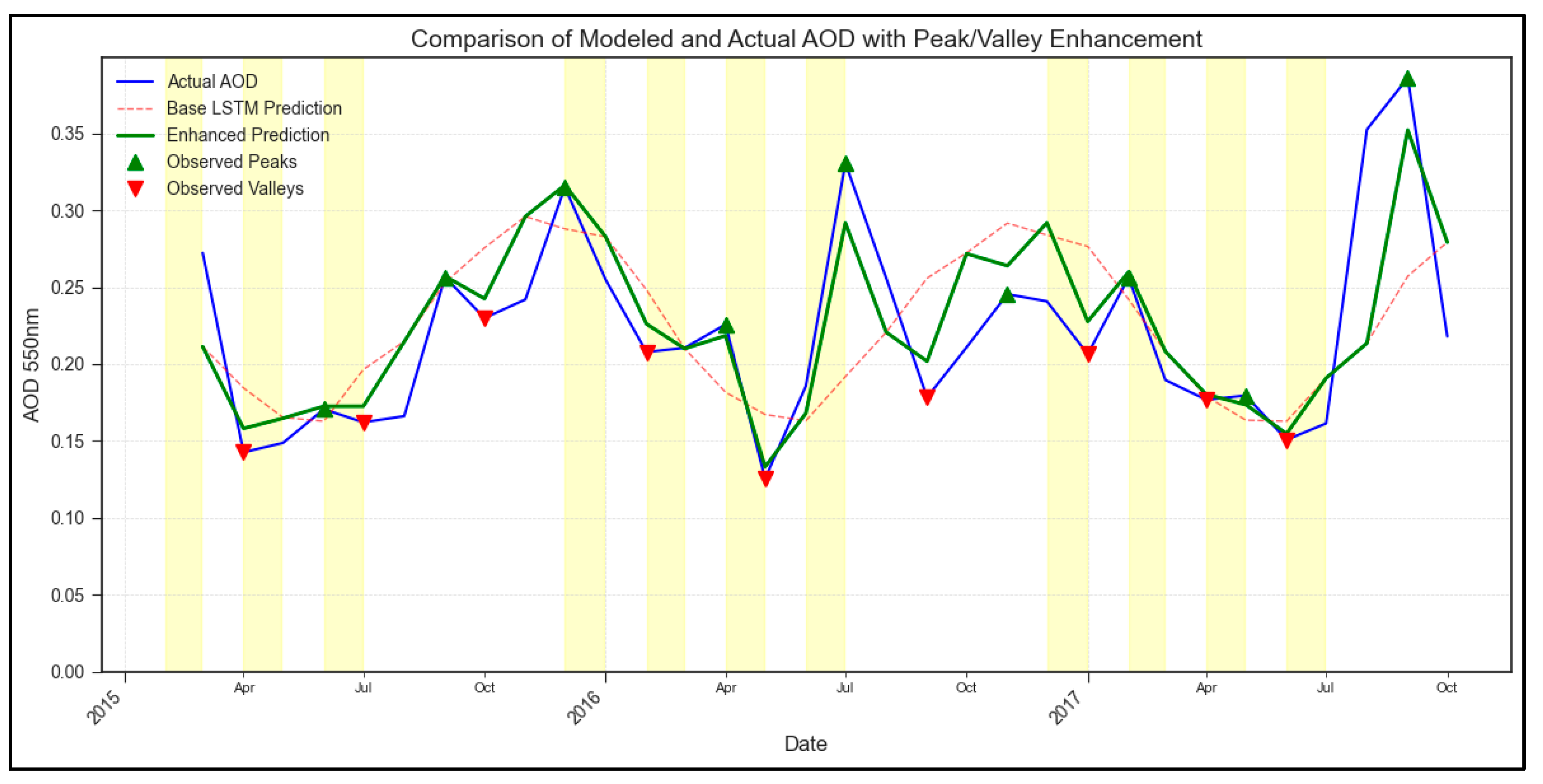
Figure 3.
Comparison of LSTM-Peak Enhanced Model on Continental Region.
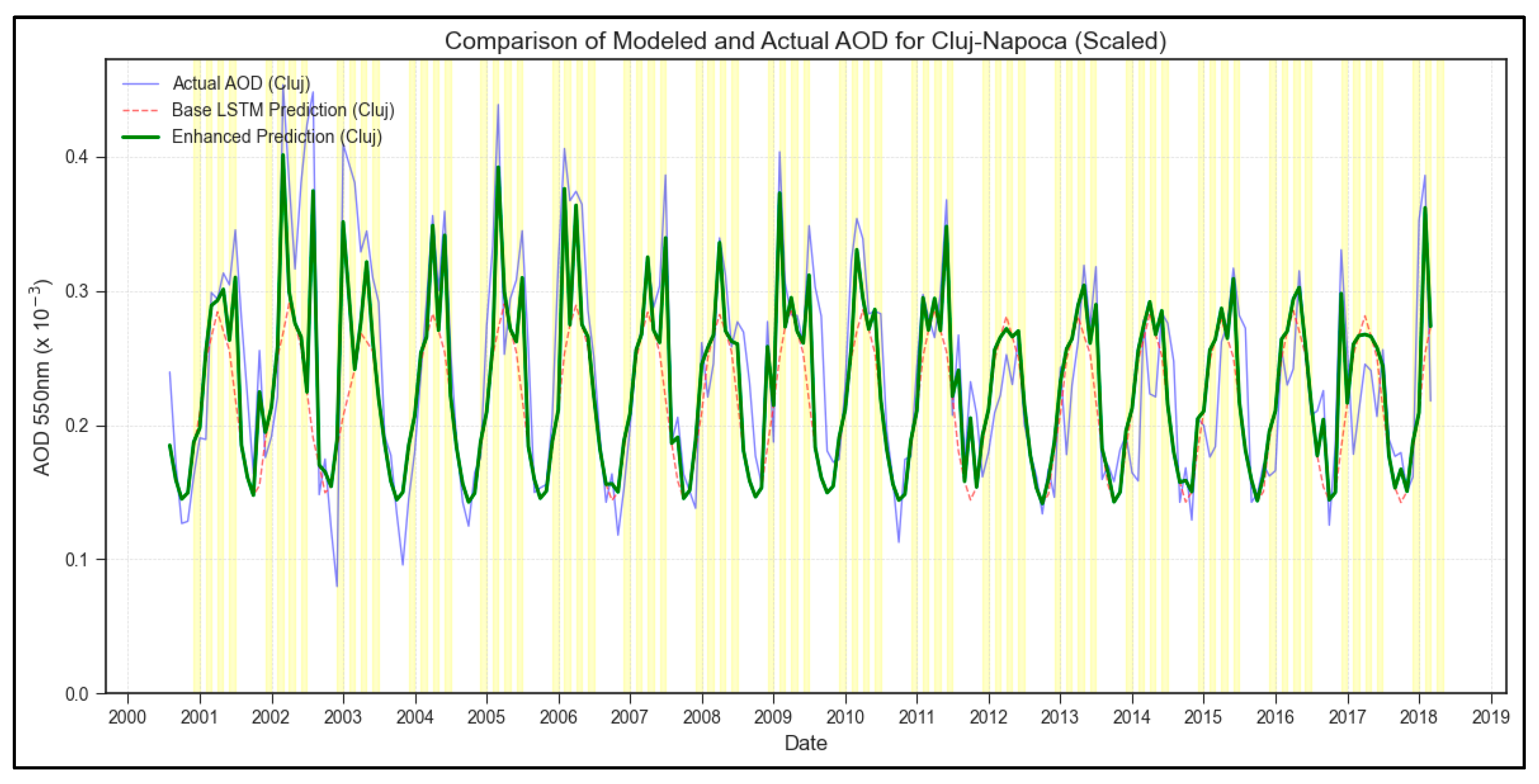
Figure 4.
Comparison of LSTM-Peak Enhanced Model on Water Region.
Disclaimer/Publisher’s Note: The statements, opinions and data contained in all publications are solely those of the individual author(s) and contributor(s) and not of MDPI and/or the editor(s). MDPI and/or the editor(s) disclaim responsibility for any injury to people or property resulting from any ideas, methods, instructions or products referred to in the content. |
© 2025 by the authors. Licensee MDPI, Basel, Switzerland. This article is an open access article distributed under the terms and conditions of the Creative Commons Attribution (CC BY) license (http://creativecommons.org/licenses/by/4.0/).
Copyright: This open access article is published under a Creative Commons CC BY 4.0 license, which permit the free download, distribution, and reuse, provided that the author and preprint are cited in any reuse.


