
Submitted:
21 April 2025
Posted:
22 April 2025
You are already at the latest version
Abstract
Carbon accumulation and structural development are key indicators of the progress of forest-ecosystem restoration. However manual techniques of measuring them are time-consuming, labor-intensive and costly. Therefore, we tested four instrument-based metrics, as potential alternatives to conventional measurements, in a control site (non-restored), reference forest and 1½- and 11½-year-old forest undergoing restoration by the framework species method (FSM). Vegetation area index (VAI) from terrestrial LiDAR, leaf area index (LAI) from a plant canopy analyser, and canopy cover from hemispherical photography (CC_HP) and a densiometer (CC_D), clearly distinguished among the control site and 1½- and 11½-year-old-restoration (<0.05) (except for CC_HP in the control plot). They correlated well (R=0.58-0.80) with manual metrics (tree stocking density (TSD), basal area (BA) and above-ground carbon (AGC)), although the correlations weakened, with increasing structural development. However, the instrument-based metrics failed to reflect a doubling in AGC between 11½-year-old restoration and the reference forest, by under-estimating increases in structural development beyond canopy closure. CC_D is recommended for monitoring structural development, during early forest restoration, due to its cost-effectiveness, ease of use and minimal disturbance of the forest understory. After canopy closure, AGC remains the most useful metric to gauge how closely restoration achieves reference-forest conditions. After 11½ years of implementing the FSM, AGC had reached 49% (65.9 tC/ha, ±SD 30.44) of the reference forest level (137.4 tC/ha, ±SD 83.19).
Keywords:
Forest landscape restoration
; Forest monitoring
; Forest carbon
; Forest structure
; Structural metrics
; Forest differentiation
1. Introduction
Throughout the tropics, efforts to restore forest ecosystems on degraded land are intensifying, as billions of trees are planted to combat biodiversity loss and to meet the ambitious targets of global and regional initiatives to tackle climate change [1,2]. As evidence accumulates that restoring tropical forest ecosystems sequesters carbon more rapidly than other land-use-change (LUC) solutions to climate change [3,4], the need for more efficient and less intrusive monitoring, to verify such results, grows.
Forest restoration usually combines assisted natural regeneration [5] with tree planting, to recover ecosystem biomass, structural complexity, biodiversity and ecological functionality close to pre-disturbance levels. Both planted and naturally regenerating trees are subject to intensive maintenance (weeding and fertilizer application) over the first two years, to initiate canopy closure, after which, the ecosystem ideally becomes self-sustaining [6]. Progress towards achieving these goals requires frequent and accurate monitoring, so that restoration methods, including species selection and maintenance regimes, can be adjusted for optimum results.
Monitoring is conventionally performed by measuring tree heights (with a pole or clinometer) and tree girth at breast height (with tape measures). When combined with species-specific wood-density data (usually obtained from online databases [7]), such ground-based measurements can be used to estimate above-ground tree carbon (AGC), using allometric equations [8,9,10]. In northern Thailand, Pothong et al. developed such equations, specifically for the forest trees of the region [11].
Such field measurements are labor-intensive, often involving large teams of people, who can inadvertently trample young tree seedlings, which could impede the forest’s future carbon-absorption capacity. Furthermore, these measurements are rooted in traditional production-forestry practices; they do not directly assess those tree components responsible for carbon absorption into the ecosystem via photosynthesis, i.e., the leaves and their arrangement in tree crowns. To anticipate future carbon-storage potential of forests undergoing restoration, it therefore makes sense to include forest-canopy metrics, as they are likely to be related to a forest’s subsequent photosynthetic capacity. Canopy cover (CC) is one such metric; the proportion of forest floor that is covered by the amalgamation of tree crowns, which form the forest canopy [12,13].
Therefore, in this paper, we compare conventional manual tree measurements with four instrument-based methods, which focus on various forest-canopy metrics: (i) vegetation area index (VAI), derived from terrestrial LiDAR point clouds [14], ii) leaf area index (LAI) [15], using a plant canopy analyser, (iii) canopy cover from hemispherical photography (CC_HP) [16]. and (iv) canopy cover, using a forest densiometer CC_D [17].
Our study also explored some of the limitations of these techniques e.g. woody elements that obscure leaves, over- or under-exposed hemispherical photos and nonuniform distribution of points in LiDAR point clouds [18,19,20].
We tested the hypothesis that forest canopy metrics, measured by the four instrument-based techniques listed above, could be used to monitor and differentiate states of restoration of upland evergreen-forest in northern Thailand.
2. Materials and Methods
2.1. Study Sites
Data were collected from 18th November to 17th December 2023 at the Mon Cham viewpoint, near the village of Nong Hoi in Chiang Mai Province, northern Thailand (18° 56´ 18.0˝ N, 98° 49´ 16.7˝ E), in the upland evergreen-forest zone, at an elevation of 1,300 m above sea level. The original vegetation of the site had been upland evergreen forest [21], which had been mostly been cleared and converted to agriculture in the 1960-70’s, subsequently abandoned, and overgrown by herbaceous weeds and grasses.
Four contrasting study sites were demarcated (Figure 1) in close proximity to one another: i) remnant undisturbed forest (reference forest [22]: RF), ii) 11½-year-old restoration forest, planted with trees in 2012 (R12), iii) 1½-year-old restoration forest, planted with trees in 2022 (R22) and iv) degraded land, dominated by herbaceous weeds, not planted for restoration (non-planted control: CT).
The framework species method (FSM) had been applied in the two restoration sites. This method of forest-ecosystem restoration involves planting tree species that are characteristic of the reference forest, which also exhibit high survival and growth rates on exposed areas, and are able to inhibit herbaceous weed growth and attract seed-dispersing animals (by producing fruits or habitat structures at a young age) [23]. The FSM is known for rapid carbon accumulation, with above ground tree carbon approaching that of reference forest within 20-30 years [24].
2.2. Conventional Manual Assessment of Above-Ground Tree Carbon Using an Allometric Model and Basal Area
In each of the four study sites, eight circular sample plots of radius 5 m were established. Within each circle, the height (m) and girth at breast height (GBH (cm) of all trees with GBH > 5 cm were measured. GBH was measured using a tape measure, whilst tree heights were determined using an extendable pole (for trees up to 10 m tall) or a clinometer (for trees taller than 10 m). GBH was converted to tree diameter at breast height (DBH) by dividing by pie.
The species of each tree was recorded by an experienced team of restoration ecologists and the species-specific wood density obtained either from Pothong et al. [11] or from the Global Wood Density Database [7]. For species with multiple published values of wood density, the species mean was used. For non-listed species, genus means were used and for those without genus means, the mean value for all northern Thailand trees in Pothong’s study was substituted (0.52 g/cm3).
The following allometric equation from Pothong et al.’s study of northern Thailand trees was used to estimate the above-ground biomass of each tree (Equation 1). We also applied an average carbon content value of 44.84% (also reported by Pothong et al. for the trees of northern Thailand). Thus, the amount of carbon stored in each tree could be estimated using equations 1 and 2.
where, AGB is an individual tree’s above-ground biomass (kg), DBH is tree diameter at breast height (cm) (GBH/pie), H is tree height (m) and WD is wood density (g/cm3). The values used for the parameters ‘a’ and ‘b’ were 0.134 and 0.847, respectively, for trees of D=1.6 to 20.0 and 0.067 and 0.976, respectively, for trees of D>20.0 cm, empirically derived by Pothong et al. [11], from felling and measuring 76 trees. AGC of all trees in each circle was summed, and the mean total/circle converted into an estimate of tons per hectare for each of the four sites.
AGB = a × (DBH2 × H ×WD)b
Above-ground Carbon (AGC) = 0.4484 × AGB
Basal area (BA) is a useful index of forest structure as it combines numbers of trees per unit area (tree stocking density, TSD) with their sizes. It is the proportion of a sample area occupied by the sum of the cross-sectional areas (1.3 m above ground) of all tree stems in the plot, expressed as m2 stems per hectare [25]. The stem cross-sectional area of each tree was calculated from the GBH measurements, mentioned above (equation 3):
where BAi is individual tree stem basal area (m2), GBH is tree girth at breast height (cm). Summation of all individual-tree BAs were used to indicate BA of each plot in m2/ha (equation 4):
BAi = GBH2 / (4π × 104)
BA = Σ BAi × (10,000 / 78.5)
2.3. Vegetation Area Index (VAI) Derived from LiDAR Point Clouds
In each of the same circular sample plots, a vegetation area index was derived from terrestrial laser scanning, using a FARO Focus core LiDAR scanner (Faro Technologies, USA), mounted on a tripod, to acquire the 3-D structure of the forest as a point cloud. The scanner was set to 1/16 resolution and 4x scan quality (each point being scanned four times) in all sample circles. Color and texture were added to the point cloud from the parallel RGB camera. The scanner was controlled by an Apple iPad Air 3 (Apple Inc., 2018) via Wi-Fi. The scans were repeated in five positions in each circle: in the plot center and on the circular plot circumference in the due north, east, south and west positions (Figure 2). This approach was recommended by Liang et al. [26] to deal with the problem of trees obscuring each other within a single scan. To combine all five scans, into a single point cloud, five references spheres were placed in fixed positions in each of the sample plots, shown in Figure 2a. These reference spheres were custom-made by placing a 20-cm sphere pole light (Luzino; Jewel P08-WH) on a 1.5-m camera stand (Figure 2b). Furthermore, the reference spheres were marked with colored masking tape, to prevent confusion during merging the scans (scan registration).
All scan data in each plot were processed using Faro SCENE software (version 2023.1.0; Faro Technologies, Inc. USA). For merging the five point-clouds in each plot, we employed the manual registration method, using reference sphere identifications [27]. During manual registration, the software positions each individual model into the main model one at a time.
At least two identical locations or objects (reference spheres in our case) must be spotted in each pair of scans (Figure 3a). Typically, the mark sphere tool was used to locate the reference sphere. However, if the sphere was obstructed, the tool can fail to fully detect it. In such cases, a mark point was used to assign the reference spot on part of the sphere or surrounding area. After registration, the merged model was trimmed to a 10 m × 10 m square, to fit the circles (5 m radius) used for AGC measurements. The point cloud was then exported in LAS format for VAI analysis.
Model analysis involved (i) model preparation [28] and (ii) index calculation [20] (Fig. 4). Model preparation was performed using the lidR package [29] in R language [30]. First, a digital terrain model (DTM) was created, using the ‘classify ground’, ‘filter ground’ and ‘rasterize terrain’ functions, sequentially. The DTM was then subjected to height normalization, using the ‘normalize height’ function to flatten the ground. Then, points lower than 1.2 m were removed, to eliminate ground flora including small tree saplings.
VAI was then calculated from the processed 3D LiDAR point cloud (Figure 4). VAI is defined as the total surface area of all vegetation components (leaves, stems, branches, etc.) per unit ground area (a dimensionless proportion) [20,28]. To calculate VAI, the number of points was observed within subsample boxes called “voxels”. For the dimensions of each voxel see equations 5 and 6.
where u is 10×res (mm) and D is the average width of the leaves (m).
where res is the model resolution (mm), R is the distance to the observed point (m), and ∆Ψ is the angular resolution of the scanner (microradian, μrad).
Voxel dimension = u(length)×u(width)×D
res = R ∙ ∆Ψ
Within each voxel, the number of points was limited to three, to address unevenness of point distributions. Subsequently, the total number of points in all voxels was multiplied by the average area of a single leaf, to calculate the VAI value of the model (equation 7) [20].
All model processing was done on a Victus 16 laptop (HP Inc., 2021) with AMD Ryzen 5 5600H CPU, NVIDIA GeForce RTX 3050 laptop GPU, and 16 GB DDR4 3200 MHz RAM.
2.4. Leaf Area Index (LAI) Using Plant Canopy Analyser
A Li-Cor LAI 2200c (Li-Cor Biosciences, Inc., USA) plant-canopy analyser was used to measure LAI values in the sample plots. The scanner compares light conditions above the canopy—A (sky)—with those below it—B (target) . Since our study employed a single optical sensor, the A readings were made using the 4A sequence shown in Table 1 [31], to measure the average light conditions of the sky (K record).
To provide shade, the sensor was placed in the operator’s shadow. All readings were done facing the same direction. How frequently the K record was made depended on sky conditions. For example, when the sky was clear and cloudless, the K record procedure was conducted hourly. However, when scattered clouds resulted in changeable sky conditions, the A and B measures were made in close succession.
The below-canopy B reading was made at the central point of each sample plot, 1.2 m above the ground. Scans were done three times in each plot with the sensor facing north. All readings in every plot were performed with the 270° view cap on (Figure 5) to avoid direct sunlight and the operator’s shade [31]. The time at which each reading was made was recorded for configuration during post-processing.
All readings from the LAI-2200c were imported into the FV2200 software (version 2.1.1; Li-Cor Biosciences, Inc., USA) via a USB cable. Corresponding K values were assigned with all configurations and parameters selected according to the sampling conditions and compared with B values to calculate LAI (equations 8 and 9).
where T(θ) is gap fraction of the given view angle (ring).
where ω (θi) is the constant weight factor for each ring, and i refers to each of the detector rings with view angle centered at θi.
2.5. Canopy Cover from Hemispherical Photography
Hemispherical photographs were taken with a digital camera (Fujifilm model X-E4; Fujifilm Corporation, Japan) fitted with a MEIKE 6.5mm F/2.0 fisheye lens (Hongkong MEIKE Digital Technology Co., Ltd, China). The camera was attached to a tripod 1.2-m above the ground at the center of each sample plot, with the lens pointing direct upwards towards the zenith. The flash socket of the camera was always positioned in the north direction. The exposure values (EV) were incrementally reduced by 0.3 until no overexposed pixels were detected on the camera screen [32]. Before every exposure, the operator positioned himself below the camera, to ensure that no extraneous elements are visible within the frame.
The photos were imported into ImageJ (version 1.48) [33] and analyzed using the Hemispherical 2.0 plug-in [16] for canopy parameter analysis. The software converted raw hemispherical photographs (Figure 6a) into black and white binarized photographs (Figure 6b). Canopy cover was calculated as the percentage of white pixels in the binarized image.
2.6. Canopy Cover from Forest Densiometer
A spherical densitometer, model A, (Forest Densiometers, USA, Figure 7a) was also used to quantify canopy cover in each sample plot. The instrument consisted of a convex mirror with a grid of 24 squares engraved upon its surface. To estimate canopy cover (CC), the instrument was leveled horizontally 1.2 m above the ground. Each square was mentally divided into quarters. The number of quarter-squares reflecting mostly sky was counted and multiplied by 1.04, to obtain an estimate of the gap-fraction per cent (because there were 96 (not 100) quarter squares in the grid) (Figure 7b). The gap-fraction per cent was subtracted from one hundred, to derive an estimate of the canopy-cover per cent (equation 10). This was repeated four times in each sample plot (facing each of the cardinal points) and the values averaged.
CC = 100 - (GF × 1.04)
3. Results
In thirty-two 5-m-radius circular sample plots, the mean values of all metrics, trended similarly across all four sites; from lowest values in the non-planted control site (CT), increasing sequentially from younger (R22) to older (R12) restoration sites and reaching maximum values in the reference forest (Table 2, S1).
Increases in mean VAI, LAI and CC_D, between CT and R22 (control and 1½ year-old restoration), were significant (P<0.05, ANOVA) and substantial (per cent increases of 157, 131 and 1,171 for VAI, LAI and CC_D respectively).
All metrics clearly distinguished between young and older restoration. Increases in all metrics between 1½ (R22) and 11½-year-old restoration (R12)—both instrument-based and manual—were significant (P<0.05) and substantial (per cent increases of 77.5, 115.0, 49.0, 45.4 for VAI, LAI, CC_HP, CC_D and 419.9, 149.0 and 335.0 for AGC, TSD and BA, respectively).
Comparing metrics between R12 and the reference forest revealed how closely structural development of the 11½ year old restoration approached that of reference forest. Instrument-based metrics in R12 had increased to 89.6-97.7% of reference-forest values by 11½ years and the small differences between R12 and RF were statistically insignificant (P>0.05). Considering the manual metrics, mean TSD in R12 was 81.3% of the RF value, whilst mean BA in R12 was 73.3% of the RF value. Again, neither of these differences were statistically significant (P>0.05) i.e. all instrument metrics, and two of the manual metrics did not clearly distinguish between advanced restoration and the reference forest. Only AGC, was significantly lower in the R12 site than in the reference forest, attaining 47.9% of the reference-forest value (in 11½ years) (P<0.05).
Figure 8a presents correlation coefficients (r), indicating the strengths of the relationships between the metrics, across all 32 plots. Most of the metrics were highly correlated with one another. Considering the question of how well instrument-based metrics (VAI, LAI, CC_HP and CC_D) might be able to replace manual ones (AGC, TSD and BA), correlations between AGC and instrument-based metrics were moderate, with CC_HP having the strongest relationship (r=0.67). However, the relationships between AGC and the other instrument-based metrics were only very slightly weaker (VAI, r=0.64; LAI, r=0.63 and CCD_D, r=0.58).
Correlations between TSD and instrument-based metrics were all stronger. The strongest relationship was with LAI (r=0.80), but it was only marginally stronger than the relationships between TSD and the other three instrument-based metrics. Correlations of instrument-based metrics with BA were also strong. The strongest relationship was with CC_HP (r=0.75), which was only slightly stronger than with the other instrument-based metrics.
Correlation coefficients within each study site, based on eight circular sample plots in each (Figure 8b-e), were generally weaker and somewhat erratic, probably due to the smaller sample sizes. Since no trees were present in the sample plots in CT, no correlations between instrument-based metrics and manual metrics could be derived (Figure 8b).
In the young restoration plot (R22), those instrument-based metrics, which had the strongest relationships with manual metrics, were CC_HP and LAI with TSD (r=0.71 and 0.65 respectively) and VAI with AGC (r=0.63) (Figure 8c). In the older restoration plot (R12), the strongest correlations between instrument-based and manual metric were between VAI with AGC (r=0.67) and BA (r=0.55) (Figure 8d). In the reference forest, correlations were weaker. CC_HP correlated most strongly with BA (r=0.42) (Figure 8e). Other correlations between instrument-based and manual metrics were much weaker.
Discussion
This study compared instrument-based metrics (VAI, LAI, CC_HP, and CC_D) with conventional metrics, derived from direct, manual, tree measurements (AGC, TSD and BA), to monitor forest structural recovery during restoration by the framework species method (FSM) [23]. The relative advantages and disadvantages of all seven metrics investigated are summarized in Table 3. The study also demonstrated the extent of development of forest structure achievable over the first decade after implementing the FSM.
4.1. Instruments and Metrics
Information content of the instrument-based metrics increased from CC_D and CC_HP (degree of canopy closure), to LAI (canopy density including beyond initial canopy closure) and VAI (canopy physical structural complexity – including leaves and branches etc.).
4.1.1. LiDAR and VAI
The advantage of terrestrial LiDAR is that it physically scans all forest structures (including leaves and branches) and combines them all into a single index—in this case VAI. Thus, the information content of the derived metric is much higher than that of the other instrument-based metrics in this study. The technique clearly distinguished differences in structural development between the CT, R22 and R12 plots, but not between the R12 and RF plots (Table 2). VAI also correlated well with all manual metrics, when considering the combined data from all plots (Figure 8a).
However, the method appeared to underestimate forest structural development in RF. VAI values in R12 and RF were statistically indistinguishable, whereas AGC in R12 was, significantly, less than half of that in RF. A problem with using terrestrial LiDAR in dense forest is that low branches and other close objects can block scanning of more distant structures, particularly those in the canopy [26,34]. This may have reduced the VAI in RF, such that the difference in mean VAI’s between R12 and RF was less than expected, when compared with the difference in AGC measurements. It might also explain the low correlation coefficients between VAI and the manual metrics in both R12 and RF (Figure 8d & e).
In an attempt to address this issue, we combined five scans per plot (Figure 2), since previous researchers have shown that using multiple scans (3-5) improves accuracy of the technique, compared to a single scan [34]. Despite this, under-estimation of VAI in RF was still apparent at the 1/16 resolution and 4x scan quality, used for this study. Higher resolutions should therefore be tested in the future, although high-resolution scanning considerably increases the fieldwork time needed.
In contrast, Ehbrecht et al. [35] successfully used single scans to generate the newly developed “stand structural complexity index” (SSCI), which holistically quantifies the spatial arrangement of plant material in forests. Furthermore, combining terrestrial and airborne LiDAR point clouds, has also generated some impressive results for capturing forest structures recently, under various environmental conditions [36].
Therefore, we recommend further studies on the effects of scanning configuration and resolution, and on combining terrestrial and aerial LiDAR point clouds.
Considering the practicalities of using LiDAR for monitoring forest-restoration progress, setting up the tripod in five locations within 10-m-diameter circles resulted in considerable trampling of tree saplings in the undergrowth, which may affect subsequent forest regeneration. The instrument, the reference spheres and their tripods are bulky and great care must be taken when transporting them and setting them up. Post-processing of point clouds involves a steep learning curve. Crucially, terrestrial LiDAR scanners are very expensive (30,000-100,000 USD). The prospect of routinely using them to verify carbon credits, for example [14], seems remote, until they become more affordable and user-friendly.
4.1.2. Plant Canopy Analyser and LAI
A plant canopy analyser uses algorithms to infer an index of canopy density indirectly from the attenuation of light, as it passes through the forest canopy; it does not register forest structure directly, like LiDAR does. An LAI of <1 indicates incomplete canopy closure; 1 indicates cover by a single layer of leaves (on average); 2 by a double layer of leaves—and so on. Even after complete canopy closure, differences in light readings between the open sky and beneath the forest canopy should increase further, with increasing canopy density, i.e. the metric should not saturate at 100% canopy cover.
LAI and VAI results were similar, in that LAI distinguished differences in canopy development between the CT, R22 and R12 plots, but not between the R12 and RF plots (Table 2). Similarly, LAI also correlated well with all manual metrics, when considering the combined data from all plots (Figure 8a). As with VAI, however, the failure of LAI to distinguish between advanced restoration (R12) and the reference forest (RF), did not reflect the more than doubling of AGC between the two sites. Furthermore, correlations with manual metrics in the denser plots (R12 and RF) were poor. Therefore, it seems that further increases in the canopy density, post-canopy-closure, are poorly related with further light attenuation.
Costing around 1000-15,000 USD, plant canopy analyzers are cheaper than LiDAR. They are easier to deploy than LiDAR, and can be used by a single observer, thus minimizing trampling of young tree seedlings. However, the need to make frequent open-sky readings (using a single sensor device) imposes difficulties. If the below-canopy sample points are far from the forest edge, the time interval between open-sky and under-canopy readings becomes unacceptably long, particularly when cloud conditions are changeable [31]. This highlights the difficulty of using a passive-sensor device under variable ambient light conditions.
4.1.3. Canopy Cover
Both the hemispherical camera and the densitometer measure canopy cover (CC) by subtracting the amount of visible sky from a ground-up view of the forest canopy and assigning remaining pixels as “canopy”. Once no sky becomes visible (i.e. complete canopy closure), however, they return a CC of 100%, no matter how many additional layers of leaves and branches grow and augment canopy density thereafter [37,38,39].
The pattern of CC_D results was the same as those of VAI and LAI. The metric distinguished between the CT, R22 and R12 plots, but not between the R12 and RF plots (Table 2). It did not reflect the doubling of AGC between R12 and RF. CC_D correlated similarly well with the manual metrics across all plots (Figure 8a). Once again, correlations with manual metrics in the denser plots (R12 and RF) were mostly very low (except for TSD in R12 r=0.48) (Figure 8d).
Hemispherical photography registered an obvious anomaly—52.1% canopy closure in the control site (CT), where no trees grew (compared with 4.8% from the densiometer) (Table 2). Although the camera’s exposure value (EV) was manually adjusted, to prevent over- or under-exposure (which may lead to errors in the CC estimation [32]), the camera still included trees at the edge of the plot in images, due to the steep slope and the wide field of view of the hemispherical lens (zenith angle = 90°) (Figure S2). To mitigate this in the future, hemispherical photos should be analyzed by other methods with smaller zenith angles, such as Can-Eye software (zenith angle = 60°), to identify vegetation cover on steep terrain with more certainty [40,41].
In common with all other instrument-based metrics CC_HP was significantly higher in R12 than in R22, but the metric failed to distinguish between R12 and RF. As with other instrument-based metrics, correlations with manual metrics weakened as structural development increased (Figure 8c-e).
The main difference between the two canopy-cover instruments is that hemispherical photography employs a precise, objective procedure to subtract sky pixels from an image, whereas readings from a densiometer are more subjective, particularly if the instrument and viewing angle are not perfectly steady. However, a densitometer can be operated by non-skilled personnel, as it simply involves counting spots on a grid. In contrast, set-up and operation of a hemispherical camera are highly technical, and post processing images requires considerable expertise and training. Furthermore, hemispherical cameras are more expensive (1200-1500 USD) than densiometers (200-300 USD).
4.2. Conventional Forest Surveys – Manual Metrics
All manual metrics were obtained from the same survey of trees of GBH>5 cm in all circular sample plots, using conventional, standard, survey techniques, carried out by teams of 5-6 people. The information content of the metrics increased from TSD (tree counts) to BA (tree counts and tree sizes (GBH)) and AGC (tree counts, sizes (GBH and height) and wood density).
Structure is built from biomass, of which 45% is carbon (Eqn.2). Therefore, as AGC increases, so should the structural complexity of the forest, as the carbon becomes partitioned among an increasing diversity of structural components. This should have been reflected by strong correlations of AGC with instrument-based metrics of structural development. In general, correlations of AGC with instrument-based metric were moderate, becoming weak in the R12 and RF plots. This may have been because calculation of AGC is sensitive to wood density (Eqn. 1), a variable which was “invisible” to all the instrument-based metrics. Furthermore, all four instrument-based metrics failed to reflect the doubling of AGC between R12 and RF, suggesting their inability to register further increases in forest structural complexity, beyond canopy closure.
It is interesting to note that correlation of manual metrics with all instrument-based metrics declined with increasing information content of the manual metrics i.e. TSD correlated most strongly with all four instrument-based metrics, followed by BA, with AGC correlating most weakly (Figure 8a). This may have been because potential sources of variability increase with information content. This assertion was supported by calculating the coefficients of variation (CV) from the data in Table 2 (standard deviation expressed as a percentage of the mean, Table S2). CVs were highest for AGC and lowest for TSD, consistently across all 3 forested sites.
The most common sources of potential error in field measurements included determining if trees on the perimeter of the circular sample plots should be counted in or not, and the difficulty of seeing tree tops for height measurements in R12 and RF, where high canopy density obscured the view. Field surveys are costly, due to high labour and transport requirements. Furthermore with the large teams of surveyors, required, trampling of young tree seedlings is inevitable, potentially impeding future understory development and carbon absorption.
4.3. Recovery of Forest Structural Complexity by the Framework Species Method
Figure 9 shows visually how effective the FSM is at restoring forest structure over the first decade following initial implementation.
The data, presented above, verify and quantify this visible recovery of forest structure. Planting of framework tree species augmented natural regeneration, to achieve an initial stocking density of 3100 stems/ha, mostly of saplings 30-60 cm tall. However, the TSD metric, included only those saplings and trees that had survived and grown large enough to attain a GBH of 5 cm of more by the survey time. By 1½ years, the R22 mean values of TSD, BA and AGC amounted to 32.7%, 16.9% and 9.2% of the mean reference-forest (RF) values (all significantly lower, P<0.05, Table 2)—due almost entirely to a few remnant forest trees that remained on the site at planting time. However, by 11½ years, the R12 mean values of TSD, BA and AGC had increased to 81.3%, 73.3% and 47.9% of the mean RF values respectively. R12 values of TSD and BA were statistically indistinguishable from RF values. However, mean AGC in the R12 plot remained significantly lower than the RF value. The result for mean AGC was remarkably close to that from another study of carbon accumulation during restoration of evergreen forest above Ban Mae Sa, 10 km to the south-east, at the same elevation also using the FSM. In that study, mean tree carbon accumulated in 12-year-old restoration plots was 49% of the mean reference forest value [42]. The close reproducibility of the result strongly suggests that during application of the FSM, carbon accumulation lags behind other metrics of structural development, with instrument-based canopy metrics approaching reference-forest values earlier than measurements of forest-carbon.
5. Conclusions
In conclusion, whilst all instrument-based techniques successfully distinguished among early restoration stages, once canopy closure reached about 85-90%, they failed to distinguish further progression towards reference forest conditions. This conclusion was also supported by the fact that correlations between instrument-based and manual metrics weakened with increasing forest structural development.
Of the four instrument-based metrics tested in our study, we recommend CC_D as the most cost-effective indicator of forest structural development, up until the point of canopy closure, for the following reasons:
- It distinguished among CT, R22, and R12 almost as well as the other metrics (Table 2).
- It correlated well with other instrument-based metrics across all plots.
- It showed comparable strength of correlation with manual metrics (R = 0.58–0.77; Figure 8a).
- A single person can operate it, thus minimizing trampling of seedlings.
- It is simple to use with minimal training.
- Results are immediate, with no need for complex post-processing.
- It cost is only a fraction of that of the other instruments evaluated.
Beyond canopy closure, however, manual measurement of AGC remains the most reliable indicator of forest structural development, combining direct measurements of tree size and wood density with stocking density. However, the high labour requirement and high cost of carbon surveys, and their potential impact on understorey development, remain as strong deterrents to its widespread use.
There remains a need for more reliable and cost-effective methods to track carbon accumulation and structural development during forest-ecosystem restoration. To avoid damaging the forest understory through ground surveys, canopy-based indices, derived from drone imagery, may offer the best solution [43].
Supplementary Materials
The following supporting information can be downloaded at the website of this paper posted on Preprints.org: Table S1. Individual sample-plot results; Figure S1. Principal component analysis of the measured values; Figure S2. Hemispherical photographs from each individual sampling plot; Table S2. Comparing variability among the metrics.
Author Contributions
Conceptualization, Waiprach Suwannarat and Watit Khokthong; Data curation, Waiprach Suwannarat, Pornpawee Laohasom and Watit Khokthong; Formal analysis, Waiprach Suwannarat, Stephen Elliott and Watit Khokthong; Funding acquisition, Stephen Elliott; Investigation, Worayut Takaew and Pornpawee Laohasom; Methodology, Waiprach Suwannarat, Stephen Elliott and Watit Khokthong; Project administration, Worayut Takaew and Watit Khokthong; Resources, Stephen Elliott, Worayut Takaew and Watit Khokthong; Software, Waiprach Suwannarat and Watit Khokthong; Supervision, Stephen Elliott and Watit Khokthong; Validation, Stephen Elliott and Watit Khokthong; Visualization, Waiprach Suwannarat and Watit Khokthong; Writing – original draft, Waiprach Suwannarat and Watit Khokthong; Writing – review & editing, Waiprach Suwannarat, Stephen Elliott and Watit Khokthong. All authors have read and agreed to the published version of the manuscript.
Funding
This research was funded by FORRU-CMU’s Small-Grant Support for Student Projects. The APC was funded by FORRU-CMU Research Group.
Acknowledgments
We thank Jutamas Jongman, Chadapohn Tashingkam, Sirui Tao and Woranart Yarangsee for helping with field work and Maxime Réjou-Méchain who provided training in LiDAR processing.
Conflicts of Interest
The author W.S. is an employee of MDPI; however, he does not work for the journal Applied Sciences at the time of submission and publication.
Abbreviations
The following abbreviations are used in this manuscript:
| AGB | Above-ground biomass |
| AGC | Above ground carbon |
| BA | Stem basal area |
| CC | Canopy cover |
| CC_D | Canopy cover from forest densiometer |
| CC_HP | Canopy cover from hemispherical photography |
| CT | Non-planted control |
| DBH | Tree diameter at breast height |
| DTM | Digital terrain model |
| EV | Exposure value |
| FSM | Framework species method |
| GBH | Tree girth at breast height |
| HP | Hemispherical photograph |
| LAI | Leaf area index |
| LiDAR | Light Detection and Ranging |
| PCA | Plant canopy analyser |
| R12 | Restoration forest planted in 2012 (11½ years old) |
| R22 | Restoration forest planted in 2022 (1½ years old) |
| RF | Reference forest |
| TLS | Terrestrial laser scanning |
| TSD | Tree stocking density |
| VAI | Vegetation area index |
References
- UN Decade on Restoration, (n.d.). The UN Decade on Restoration. https://www.decadeonrestoration.org/ (accessed on 2nd February 2025).
- FAO. (2024). RESULT Asia-Pacific: Restoring and Sustaining Landscapes Together – A Regional Programmatic Framework for Forest and Landscape Restoration. Rome: Food and Agriculture Organization of the United Nations. 79 pp.
- Sacco, A.D.; Hardwick, K.A.; Blakesley, D.; Brancalion, P.H.S.; Breman, E.; Rebola, L.C.; Chomba, S.; Dixon, K.; Elliott, S.; Ruyonga, G.; et al. Ten golden rules for reforestation to optimize carbon sequestration, biodiversity recovery and livelihood benefits. Global Change Biology 2021, 27, 1328–1348. [Google Scholar] [CrossRef] [PubMed]
- Jantawong, K.; Kavinchan, N.; Wangpakapattanawong, P.; Elliott, S. Financial Analysis of Potential Carbon Value over 14 Years of Forest Restoration by the Framework Species Method. Forests 2022, 13. [Google Scholar] [CrossRef]
- Shono, K.; Cadaweng, E.A.; Durst, P.B. Application of Assisted Natural Regeneration to Restore Degraded Tropical Forestlands. Restor. Ecol. 2007, 15, 620–626. [Google Scholar] [CrossRef]
- Elliott, S.D., D. Blakesley & K. Hardwick, 2013. Restoring Tropical Forests: a Practical Guide. Royal Botanic Gardens, Kew; 344 pp.
- Zanne, Amy E.; Lopez-Gonzalez, G.; Coomes, David A. et al. (2009). Data from: Towards a worldwide wood economics spectrum [Dataset]. Dryad. [CrossRef]
- Chave, J.; Réjou-Méchain, M.; Burquez, A.; Chidumayo, E.; Colgan, M.S.; Delitti, W.B.C.; Duque, A.; Eid, T.; Fearnside, P.; Goodman, R.C.; et al. Improved allometric models to estimate the aboveground biomass of tropical trees. Global Change Biology 2014, 20. [Google Scholar] [CrossRef]
- Liu, B.; Bu, W.; Zang, R. Improved allometric models to estimate the aboveground biomass of younger secondary tropical forests. Global Ecology and Conservation 2023, 41. [Google Scholar] [CrossRef]
- Pati, P.K.; Kaushik, P.; Khan, M.L.; Khare, P.K. Allometric equations for biomass and carbon stock estimation of small diameter woody species from tropical dry deciduous forests: Support to REDD+. Trees, Forests and People 2022, 9.
- Pothong, T.; Elliott, S.; Chairuangsri, S.; Chanthorn, W.; Shannon, D.P.; Wangpakapattanawong, P. New allometric equations for quantifying tree biomass and carbon sequestration in seasonally dry secondary forest in northern Thailand. New Forests 2022, 53, 17–36. [Google Scholar] [CrossRef]
- Jennings, S.; Brown, N.; Sheil, D. Assessing Forest Canopies and Understorey Illumination: Canopy Closure, Canopy Cover and Other Measures. Forestry 1999, 71, 59–73. [Google Scholar] [CrossRef]
- Seidel, D.; Fleck, S.; Leuschner, C.; Hammett, T. Review of ground-based methods to measure the distribution of biomass in forest canopies. Annals of Forest Science 2011, 68, 225–244. [Google Scholar] [CrossRef]
- Suwannarat, W.; Suwanprasert, S.; Pothong, T.; Kullasoot, S.; Sapewisut, P.; Kasithikasikham, R.; Phalaraksh, C.; Khokthong, W.; Sareein, N. Forest Carbon Estimation Using Two Vegetation Structural Indices Derived from Terrestrial Laser Scanner: VegetationArea Index and Leaf Area Index. Chiang Mai Journal of Science 2024, 51. [Google Scholar]
- Chianucci, F.; Macfarlane, C.; Pisek, J.; Cutini, A.; Casa, R. Estimation of foliage clumping from the LAI-2000 Plant Canopy Analyser: effect of view caps. Trees 2 0147, 29, 355–366. [Google Scholar] [CrossRef]
- Beckschäfer, P. Hemispherical_2.0 – Batch processing hemispherical and canopy photographs with ImageJ – User Manual; Chair of Forest Inventory and Remote Sensing, Georg-August-Universität Göttingen, Germany: 2015.
- Russavage, E.; Thiele, J.; Lumbsden-Pinto, J.; Schwager, K.; Green, T.; Dovciak, M. Characterizing Canopy Openness in Open Forests: Spherical Densiometer and Canopy Photography Are Equivalent but Less Sensitive than Direct. Journal of Forestry 2021, 119, 130–140. [Google Scholar] [CrossRef]
- Loffredo, N.; Sun, X.; Onda, Y. DHPT 1.0: New software for automatic analysis of canopy closure from under-exposed and over-exposed digital hemispherical photographs. Computers and Electronics in Agriculture 2016, 125, 39–47. [Google Scholar] [CrossRef]
- Černý, J.; Pokorný, R.; Haninec, P.; Bednář, P. Leaf Area Index Estimation Using Three Distinct Methods in Pure Deciduous Stands. J. Vis. Exp. 2019, 150. [Google Scholar]
- Taheriazad, L.; Moghadas, H.; Sanchez-Azofeifa, A. Calculation of leaf area index in a Canadian boreal forest using adaptive voxelization and terrestrial LiDAR. International Journal of Applied Earth Observation and Geoinformation 2019, 83. [Google Scholar] [CrossRef]
- Maxwell, J.F.; Elliott, S.D. Vegetation and Vascular Flora of Doi Sutep-Pui National Park, Northern Thailand; Biodiversity Research and Training Program (BRT): Bangkok, Thailand, 2001. [Google Scholar]
- Gann, G.D.; McDonald, T.; Walder, B.; Aronson, J.; Nelson, C.R.; Jonson, J.; Hallett, J.G.; Eisenberg, C.; Guariguata, M.R.; Liu, J.; et al. International principles and standards for the practice of ecological restoration. Second edition. Restor. Ecol. 2019, 27, S1–S46 [CrossRef]. [Google Scholar]
- Elliott, S., N.I.J. Tucker, D. Shannon & P. Tiansawat, 2022. The framework species method—harnessing natural regeneration to restore tropical forest ecosystems. Phil. Trans. R. Soc. B37820210073. [CrossRef]
- Jantawong, K.; Elliott, S.; Wangpakapattanawong, P. Above-Ground Carbon Sequestration during. Open Journal of Forestry 2017, 7, 157–171. [Google Scholar] [CrossRef]
- Bettinger, P.; Boston, K.; Siry, J.P.; Grebner, D.L. Valuing and Characterizing Forest Conditions. In Forest Management and Planning (Second Edition); Academic Press: 2017; pp. 21-63.
- Liang, X.; Kankare, V.; Hyyppä, J.; Wang, Y.; Kukko, A.; Haggrén, H.; Yu, X.; Kaartinen, H.; Jaakkola, A.; Guan, F.; et al. Terrestrial laser scanning in forest inventories. ISPRS Journal of Photogrammetry and Remote Sensing 2016, 115, 63–77. [Google Scholar] [CrossRef]
- SCENE 2022 FARO Focus Laser Scanners Training Workbook; 2022.
- Atkins, J.W.; Bohrer, G.; Fahey, R.T.; Hardiman, B.S.; Morin, T.H.; Stovall, A.E.L.; Zimmerman, N.; Gough, C.M. Quantifying vegetation and canopy structural complexity from terrestrial LiDAR data using the forestr r package. Methods in Ecology and Evolution 2018, 9, 2057–2066. [Google Scholar] [CrossRef]
- Roussel, J.-R.; Auty, D.; Coops, N.C.; Tompalski, P.; Goodbody, T.R.H.; Meador, A.S.; Bourdon, J.-F.; Boissieu, F.d.; Achim, A. lidR: An R package for analysis of Airborne Laser Scanning (ALS) data. Remote Sensing of Environment 2020, 251. [Google Scholar] [CrossRef]
- R: A language and environment for statistical computing. Available online: (accessed on: 2nd Febuary 2025).
- LAI-2200C plant canopy analyser instruction manual. Available online: (accessed on: 2nd Febuary 2025).
- Beckschäfer, P.; Seidel, D.; Kleinn, C.; Xu, J. On the exposure of hemispherical photographs in forests. iForest - Biogeosciences and Forestry 2013, 6, 228–237. [Google Scholar] [CrossRef]
- Schneider, C.A.; Rasband, W.S.; Eliceiri, K.W. NIH Image to ImageJ: 25 years of image analysis. Nature Methods 2012, 9, 671–675. [Google Scholar] [CrossRef] [PubMed]
- Torralba, J.; Carbonell-Rivera, J.P.; Ruiz, L.Á.; Crespo-Peremarch, P. Analyzing TLS Scan Distribution and Point Density for the Estimation of Forest Stand Structural Parameters. Forests 2022, 13. [Google Scholar] [CrossRef]
- Ehbrecht, M.; Schall, P.; Ammer, C.; Seidel, D. Quantifying stand structural complexity and its relationship with forest management, tree species diversity and microclimate. Agricultural and Forest Meteorology 2017, 242, 1–9. [Google Scholar] [CrossRef]
- Zhang, J.; Wang, J.; Cheng, F.; Ma, W.; Liu, Q.; Liu, G. Natural forest ALS-TLS point cloud data registration without control points. Journal of Forestry Research 2023, 34, 809–820. [Google Scholar] [CrossRef]
- Dassot, M.; Constant, T.; Fournier, M. The use of terrestrial LiDAR technology in forest science: application fields, benefits and challenges. Annals of Forest Science 2011, 68, 959–974. [Google Scholar] [CrossRef]
- Huete, A.R. Vegetation Indices, Remote Sensing and Forest Monitoring. Geography Compass 2012, 6, 513–574. [Google Scholar] [CrossRef]
- Pretzsch, H.; Río, M.d.; Biber, P.; Arcangel, C.; Bielak, K.; Brang, P.; Dudzinska, M.; Forrester, D.I.; Klädtke, J.; Kohnle, U.; et al. Maintenance of long-term experiments for unique insights into forest growth dynamics and trends: review and perspectives. European Journal of Forest Research 2019, 138, 165–185. [Google Scholar] [CrossRef]
- Khokthong, W.; Zemp, D.C.; Irawan, B.; Sundawati, L.; Kreft, H.; Hölscher, D. Drone-Based Assessment of Canopy Cover for Analyzing Tree Mortality in an Oil Palm Agroforest. Frontiers in Forests and Global Change 2019, 2. [Google Scholar] [CrossRef]
- Weiss, M.; Baret, F. Can_Eye v6.4.91 User Manual. 2017.
- FORRU-CMU, 2025, unpublished report. Chiang Mai University, Thailand. https://www.forru.org/projects/the-bkind-project-supporting-forest-ecosystem-restoration-in-the-upper-mae-sa-valley (accessed on 15th April 2025).
- Spiers, A.I., Scholl, V.M., McGlinchy, J. Balch, J., Cattau, M.E., 2025. A review of UAS-based estimation of forest traits and characteristics in landscape ecology. Landsc Ecol 40, 29 (2025). [CrossRef]
Figure 1.
Sample-plot locations at Mon Cham, within each of the four study sites: RF (the reference forest, 0.68 ha), R12 (restoration forest planted in 2012, 0.51 ha), R22 (restoration forest planted 2022, 1.26 ha) and in CT (non-planted control site, 0.23 ha).
Figure 1.
Sample-plot locations at Mon Cham, within each of the four study sites: RF (the reference forest, 0.68 ha), R12 (restoration forest planted in 2012, 0.51 ha), R22 (restoration forest planted 2022, 1.26 ha) and in CT (non-planted control site, 0.23 ha).
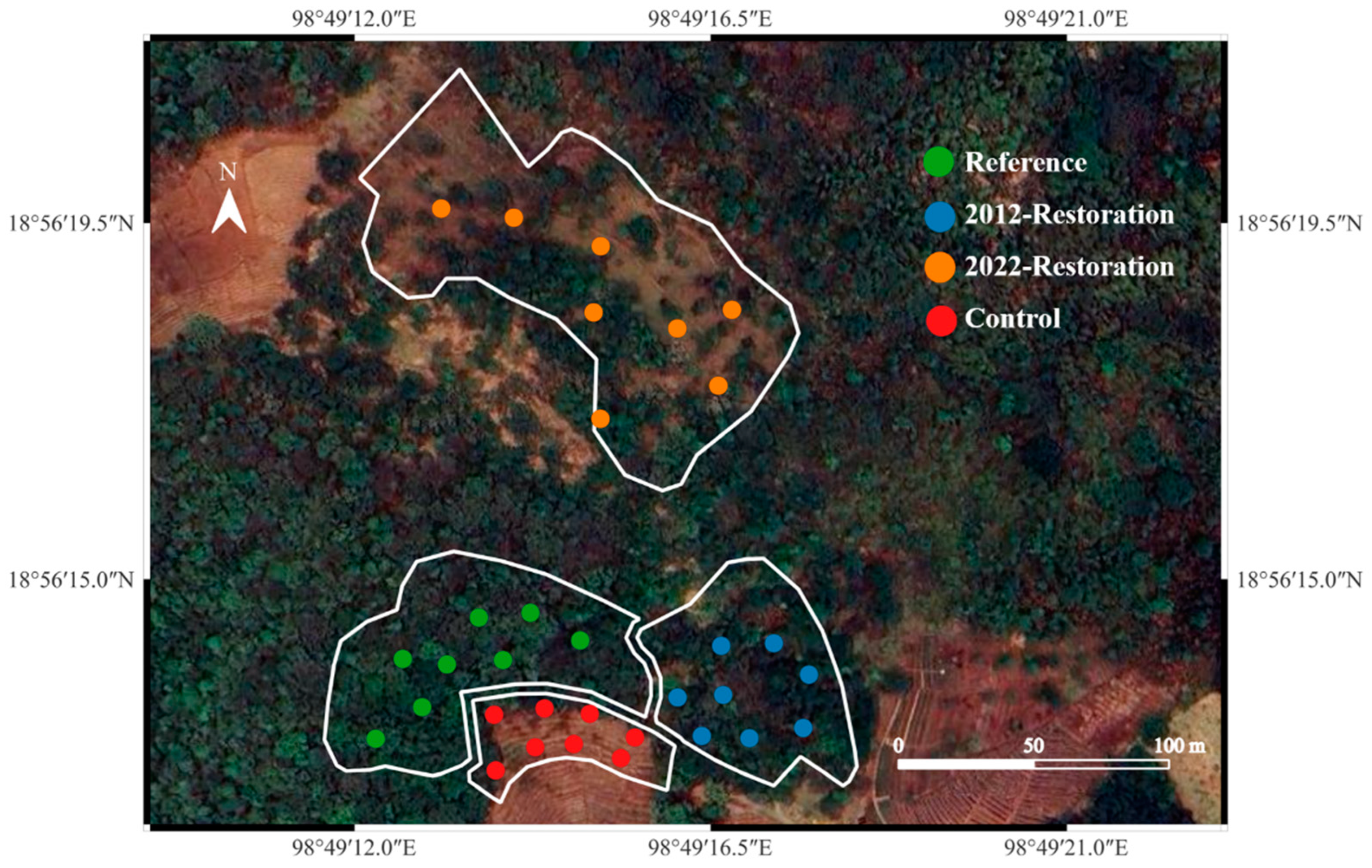
Figure 2.
(a) Setup for measurements in each 5-m radius sample plot. Measurements at the central point of each plot were made by LiDAR, PCA, forest densiometer, hemispherical photography (HP). (b) one of the reference spheres used for merging LiDAR point clouds.
Figure 2.
(a) Setup for measurements in each 5-m radius sample plot. Measurements at the central point of each plot were made by LiDAR, PCA, forest densiometer, hemispherical photography (HP). (b) one of the reference spheres used for merging LiDAR point clouds.
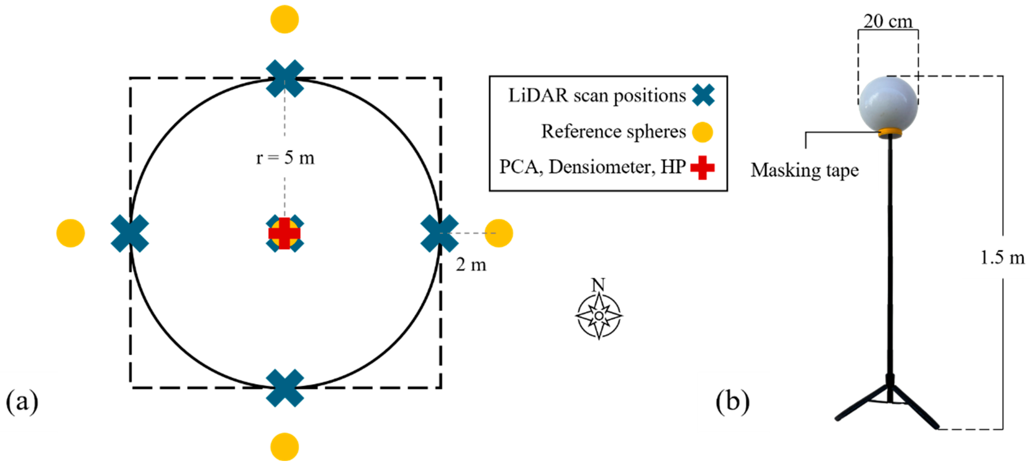
Figure 3.
(a) Two reference spheres spotted in both scan points of view; (b) the classified and flattened model.
Figure 3.
(a) Two reference spheres spotted in both scan points of view; (b) the classified and flattened model.
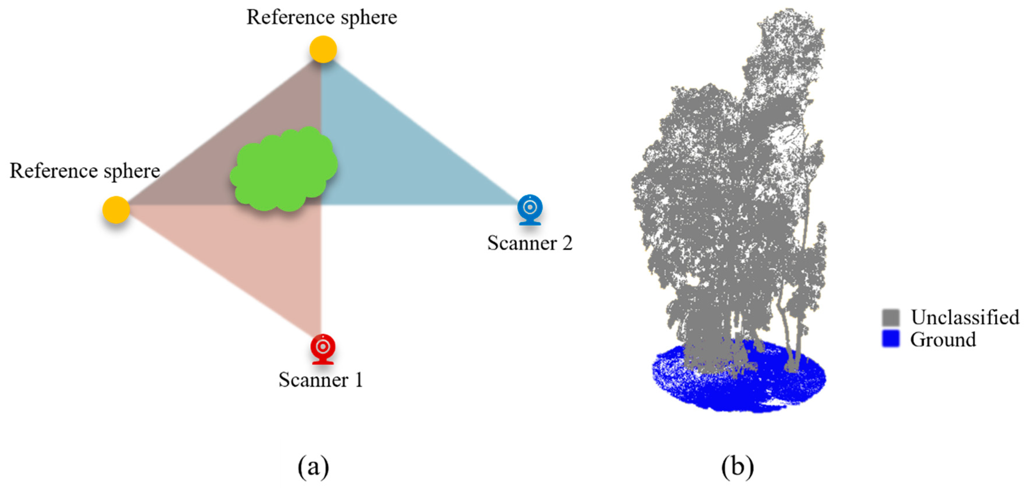
Figure 4.
Workflow of VAI calculation from a point cloud model, obtained with a terrestrial LiDAR scanner. Upper; model preparation, lower; index calculations. Here, u is ten times the resolution (10×res; mm), and D is the average width of the leaves (m).
Figure 4.
Workflow of VAI calculation from a point cloud model, obtained with a terrestrial LiDAR scanner. Upper; model preparation, lower; index calculations. Here, u is ten times the resolution (10×res; mm), and D is the average width of the leaves (m).
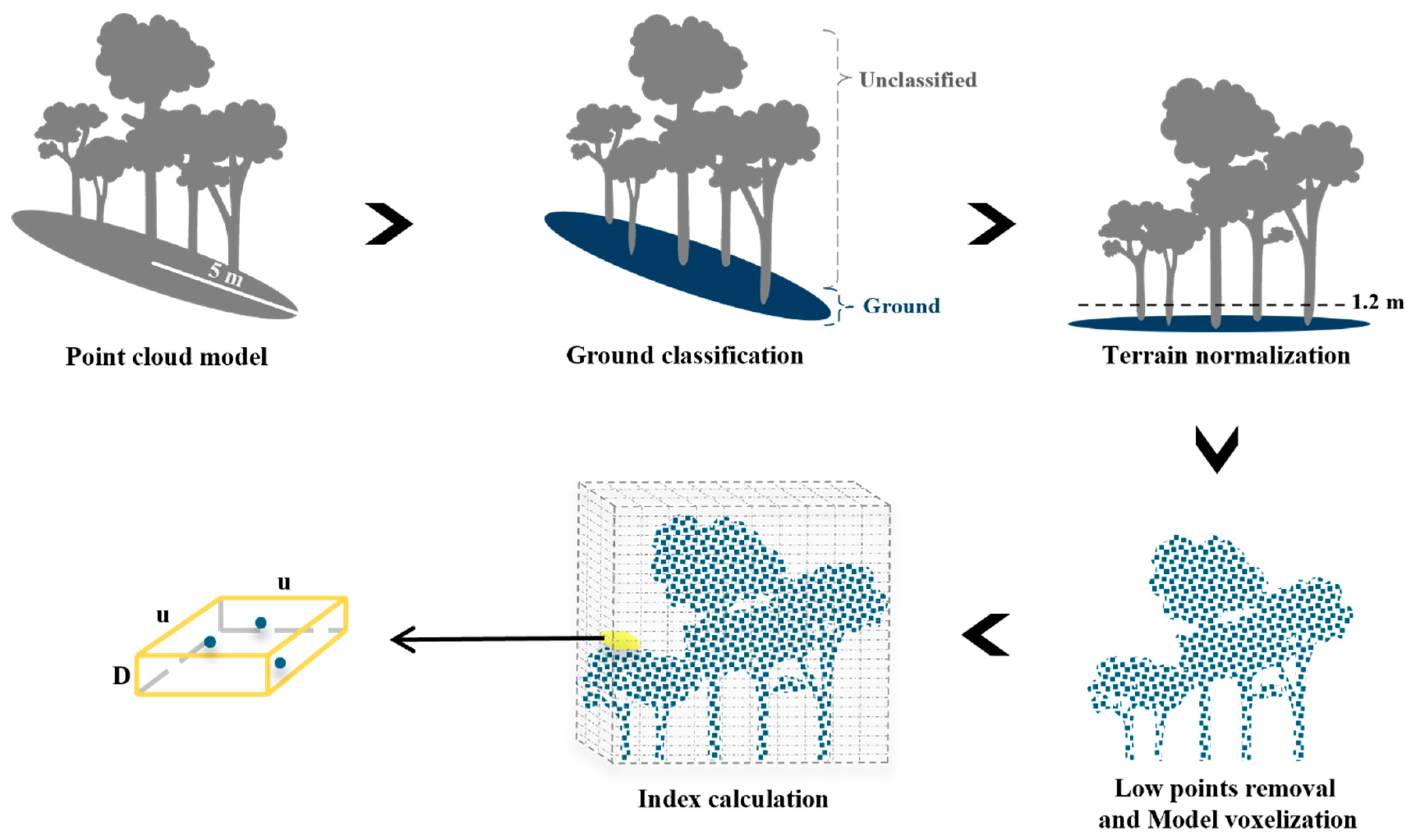
Figure 5.
View caps.
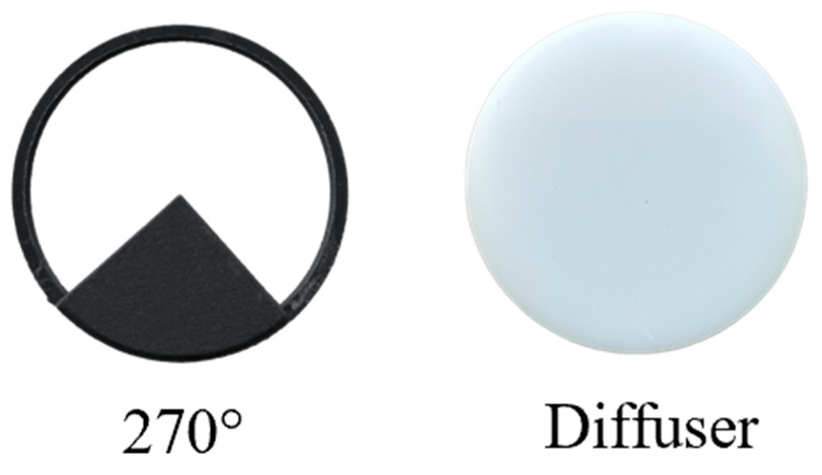
Figure 6.
(a) an input hemispherical photograph from the fisheye lens from the R22-10 plot, captured on November 18, 2023; (b) the corresponding output binarized-hemispherical photograph for gap-fraction analysis (black = sky; white = canopy).
Figure 6.
(a) an input hemispherical photograph from the fisheye lens from the R22-10 plot, captured on November 18, 2023; (b) the corresponding output binarized-hemispherical photograph for gap-fraction analysis (black = sky; white = canopy).
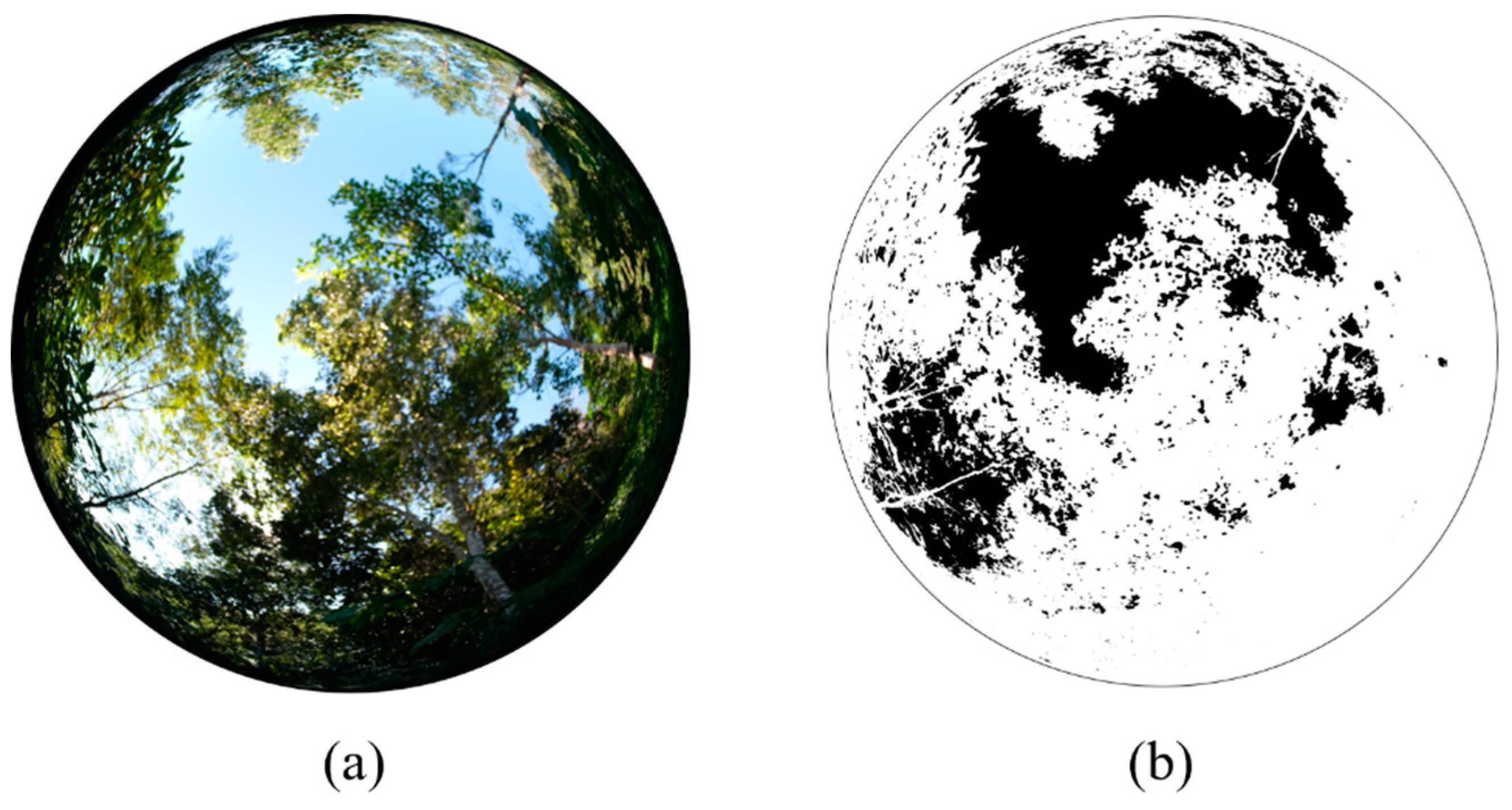
Figure 7.
(a) Forest densiometer model A; (b) example of forest densiometer corners counted (red dots) in the R12-5 plot taken on November 18, 2023.
Figure 7.
(a) Forest densiometer model A; (b) example of forest densiometer corners counted (red dots) in the R12-5 plot taken on November 18, 2023.
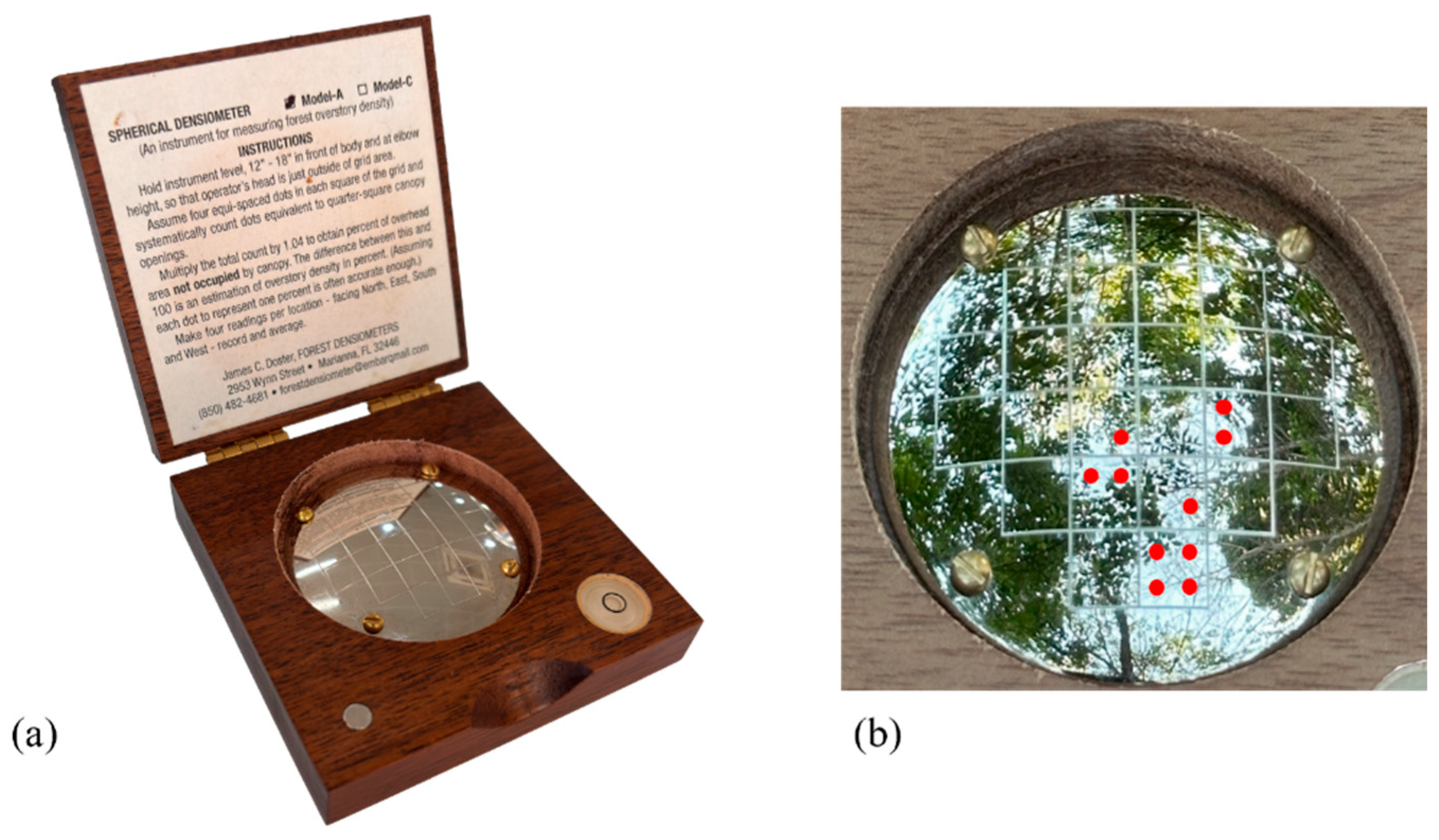
Figure 8.
Correlation coefficient (r) matrices among all metrics; four instrument based: vegetation area index (VAI) from terrestrial laser scanning, leaf area index (LAI) from a plant canopy analyser (PCA), and canopy cover from hemispherical photography (CC_HP) and a densitometer (CC_D), and three manual: above ground tree carbon (AGC), tree stocking density (TSD) and basal area (BA). .
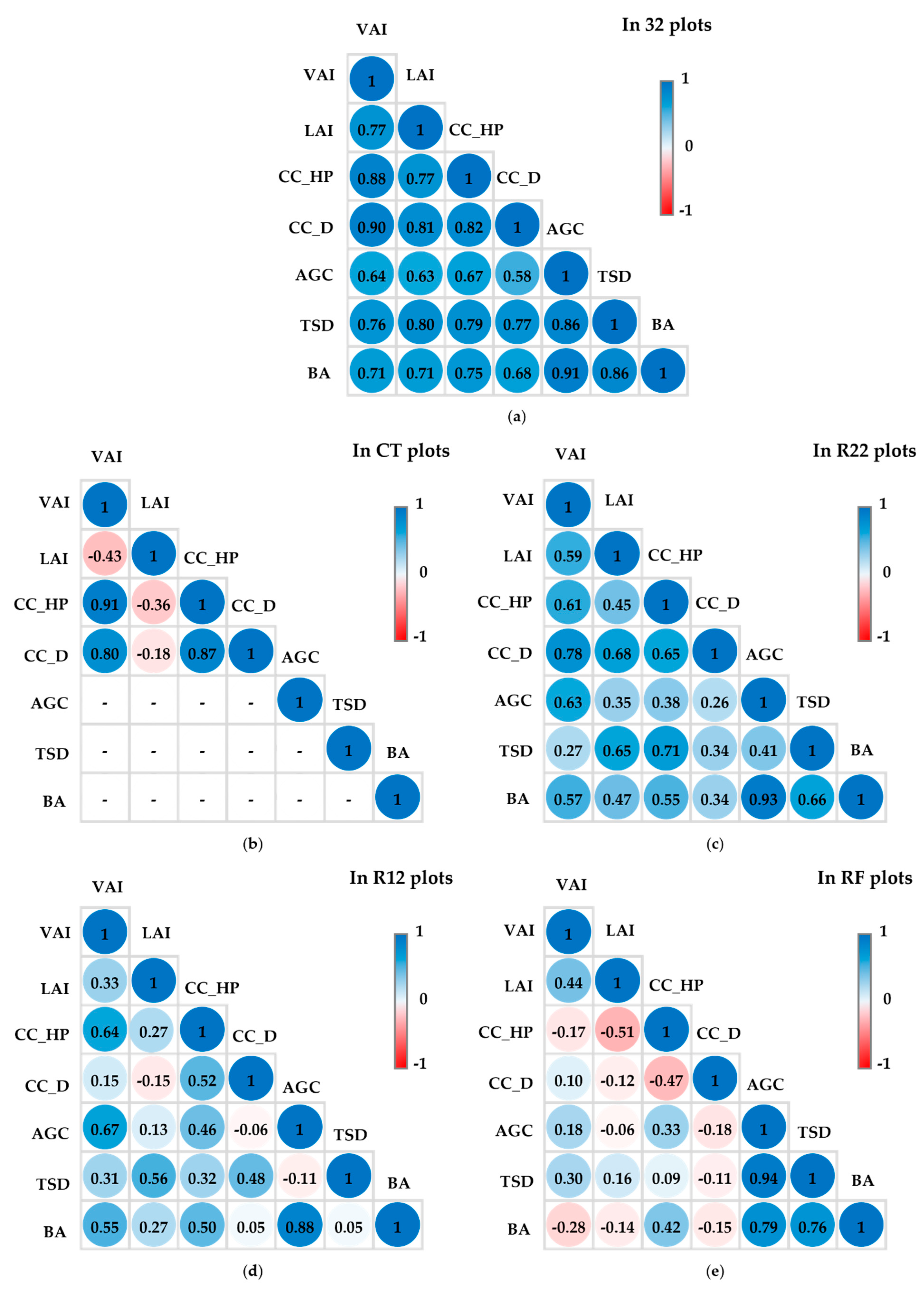
Figure 9.
(a) Initial conditions at the R12 restoration site on planting day (28/07/2012), with the edge of the adjacent reference forest (RF) visible top left. Note the landmark bamboo clump lower left. (b) A closer view of the same site 11½ years later (08/11/2023). The restored forest (right) is almost indistinguishable from the reference forest (left). .
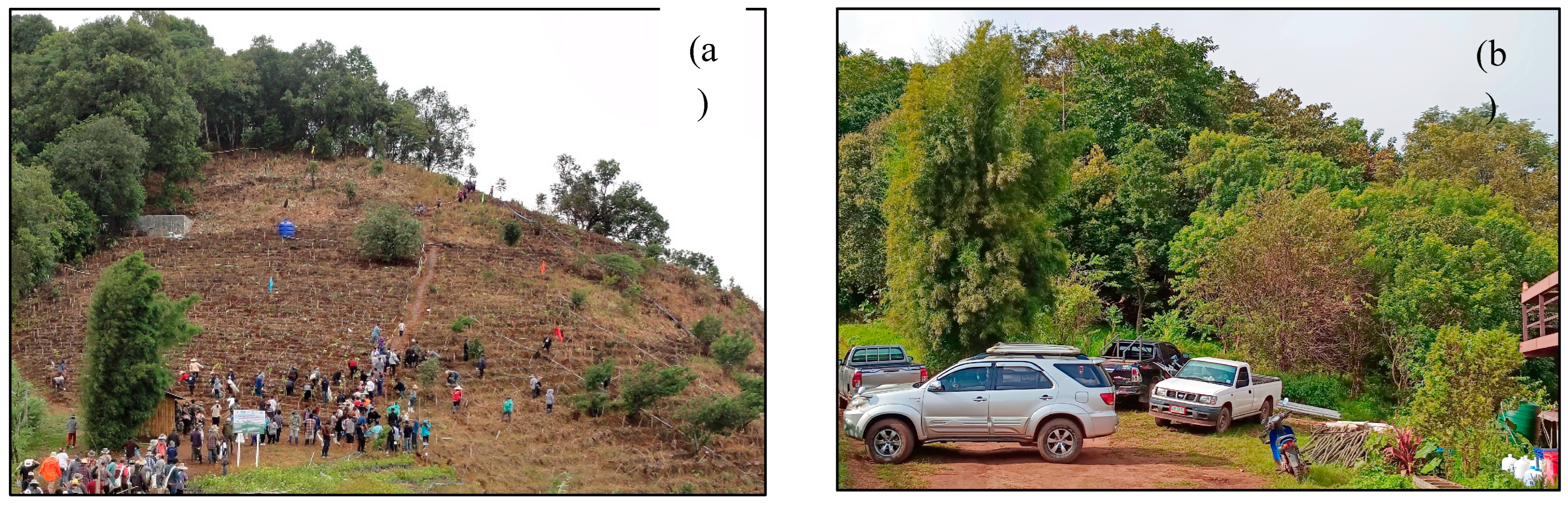

Table 1.
Attachments and readings for the 4A sequence used to compile the K record.
| Reading | Attachments | |
|---|---|---|
| # | Diffuser | Shade |
| 1 | ✓ | - |
| 2 | ✓ | ✓ |
| 3 | - | - |
| 4 | - | ✓ |
Table 2.
Mean metric values and one-way ANOVA results from each sampling site. CT; non-planted control, R22; restoration forest planted in 2022, R12; restoration forest planted in 2012 and RF; reference forest. VAI=vegetation area index; LAI=leaf area index; CC_HP and CC_D are canopy cover by hemispherical photography and densiometer respectively; AGB and AGC are above-ground biomass and carbon; TSD= tree stockings density and BA= basal area.
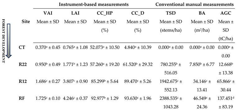
Values not sharing the same superscript are significantly different among sites (p < 0.05).
Table 3.
The pros and cons of four instrument-based and three manual metrics for tracking progress of forest-structure development during forest-ecosystem restoration.
Table 3.
The pros and cons of four instrument-based and three manual metrics for tracking progress of forest-structure development during forest-ecosystem restoration.
| Method | Metric | Cost | Labour required | Time needed | Trampling risk | Advantages | Disadvantages |
|---|---|---|---|---|---|---|---|
| LiDAR | Vegetation area Index (VAI) |
Very high (equipment) | Moderate | High ≅ manual survey | High if multiple scans | Direct scanning of all forest structures | Bulky. Complicated set-up. Steep learning curve. Obstruction by low objects may necessitate multiple scans. |
| Plant canopy analyser | Leaf area index (LAI) |
Moderate | Low | Moderate | Moderate | Takes into account increases in canopy density beyond canopy closure. Compact. | Only considers leaf canopy. Frequent open-sky readings are needed when there are scattered clouds. |
| Hemispherical camera | Canopy cover (CC_HP) | Moderate | Low | Moderate | Low to moderate | Compact. Objective and precise. | Fiddly set-up and exposure settings. Disregards multiple leaf layers beyond canopy closure. Saturates at 100%. |
| Densiometer | Canopy cover (CC_D) |
Low | Low | Low | Low | Very compact and lightweight. | Subjective readings. Disregards multiple leaf layers beyond canopy closure. Saturates at 100%. |
| Manual forest survey |
Above-ground carbon (AGC) |
High (labour/ transport) |
High | High | Very high | Well-established direct measurements. All derived from the same dataset. Results are comparable with other studies. Cheap materials and equipment. | High cost due to high labour/transport requirements. Does not include canopy measurements. |
| Tree stocking density (TSD) | |||||||
| Basal area (BA) |
Disclaimer/Publisher’s Note: The statements, opinions and data contained in all publications are solely those of the individual author(s) and contributor(s) and not of MDPI and/or the editor(s). MDPI and/or the editor(s) disclaim responsibility for any injury to people or property resulting from any ideas, methods, instructions or products referred to in the content. |
© 2025 by the authors. Licensee MDPI, Basel, Switzerland. This article is an open access article distributed under the terms and conditions of the Creative Commons Attribution (CC BY) license (http://creativecommons.org/licenses/by/4.0/).
Copyright: This open access article is published under a Creative Commons CC BY 4.0 license, which permit the free download, distribution, and reuse, provided that the author and preprint are cited in any reuse.


