
Submitted:
22 April 2025
Posted:
22 April 2025
You are already at the latest version
Abstract
Manufacturing aluminum alloy by selective laser melting (SLM) is actively imple-mented in various industries, allowing to reduce the cost of the final product and the time to market. Despite the long existence of the technology, there are still problems associated with improving the quality of SLM products, particularly those with thin walls. The purpose of our work is to study the effect of heat treatment temperatures at temperatures from 260 ºC to 530 ºC for one hour on the tensile mechanical properties, hardness and surface roughness of thin-walled samples made by selective laser melt-ing technology from Al-Mn-Mg-Ti-Zr alloy. Monte Carlo statistical analysis and mod-eling methods were used as the main method of theoretical research.
Statistical analysis of the surface roughness of thin-walled specimens manu-factured by SLM technology showed that there were no statistically significant dif-ferences (p-value>0.05) in the specimens before heat treatment and after heat treat-ment. However, data separation by hierarchical clustering method allowed us to es-tablish the presence of strong correlations between roughness parameter Rz and mi-crohardness in the group of samples heat-treated at 530 ºC. The construction and analysis of the centrality of the correlation graphs shows that the parameter with the largest number of statistically significant correlations changes with increasing heat treatment temperature. At temperatures up to 290 ºC the parameter with the largest number of correlations is the strain hardening coefficient, at temperatures from 320 ºC to 500 ºC the Young's modulus becomes the most significant, and at 530 ºC - Rz after heat treatment. The analysis of regression equations for predicting the strain hardening coefficient, Young's modulus and Rz after heat treatment with maximum centrality showed that of all mechanical properties considered in our work, the strength limit, strain corresponding to the strength limit, Young's modulus, modulus along the secant of 0.05% - 0.25% strain and strain hardening coefficient are the most significant. Mod-eling of these values depending on the heat treatment temperature with subsequent validation of the results showed that the new approach to the prediction of physical quantities presented in our work based on the Monte Carlo method gives a better prediction of the experimental results, compared to the empirical equations based on robust regression the only exception is the prediction of the strain hardening coeffi-cient.
Metallographic and X-ray phase analysis in conjunction with the results of sta-tistical analysis showed that at increasing the temperature of heat treatment mi-cropores (macrodefects) shift to the boundary of the melt zones with subsequent exit to the surface, which together with the formation of intermetallic phase and the release of titanium and zirconium leads to strain hardening of thin-walled samples obtained by selective laser melting of Al-Mn-Mg-Ti-Zr alloy.
As a result of this work, it was found that the maximum strain hardening of thin-walled specimens obtained by selective laser melting technology from Al-Mn-Mg-Ti-Zr alloy is achieved at a heat treatment temperature of 530 ºC within an hour, and the mechanism of hardening has a dual character of dispersion and due to the reduction of macro-defectivity.
Keywords:
Aluminum
; mechanical properties
; heat treatment
; hardness
; statistical analysis
; SLM
; Al-Mn-Mg-Ti-Zr alloy
1. Introduction
Additive manufacturing technologies are actively used in various industries, allowing to create high quality products and reduce the cost of production by reducing the time spent on the process “from idea to final product”. In the manufacture of metal products, the most widespread, at present, additive manufacturing technology is the technology of selective laser melting (SLM) [1,2,3,4,5,6,7,8]. Powder metals and alloys of various compositions are used as a basis for manufacturing parts using SLM technology; aluminum-based alloys and aluminum-manganese-magnesium (Al-Mn-Mg) alloys alloyed with various transition metals are most used for manufacturing parts of various shapes.
The main advantage of this alloy is its relatively low weight, complex combination of physico-mechanical properties, as well as low production cost [9,10]. On the other hand, the disadvantage of Al-Mn-Mg-based alloys is their low crack resistance, which is expressed in the appearance of many microcracks in parts obtained by the SLM technology method. This problem is solved by dispersion strengthening with intermetallic phases such as Al3M (where M is transition metal), which are formed in aluminum alloys during heat treatment, but these phases have low temperature stability [11]. To increase the temperature stability of these intermetallic phases in the temperature range from 250 °C to 350 °C, some scientists propose using elements such as scandium (Sc), zirconium (Zr), and/or erbium (Er) however, their high cost does not allow for wide use in practice [12,13,14,15]. Furthermore, a practically uniform distribution of dispersed intermetallic inclusions has been observed at 300 ºC - 425 ºC in the presence of silicon. Thus, hardening in silumins (for example, AlSi10Mg) is achieved due to the precipitation mechanism and uniform distribution of silicon at the boundary of the α-solid solution of aluminum after heat treatment at a temperature of ~270 ºС [16,17,18,19,20]. In general, both hardening mechanisms contribute to creep resistance, which is one of the most significant parameters for alloy applications at elevated temperatures [21,22,23]. In aluminum alloys, dislocation creep occurs at 250 ºC - 350 ºC [23,24,25] and there are four main ways to improve the dislocation creep resistance [26]:
- mechanical inhibition of dislocation motion;
- anchoring of dislocations by dissolved atoms;
- counteraction of dislocation motion by interactions between atoms;
- increasing the density of dislocations, leading to their intertwining.
All the above mechanisms are related in one way or another to the cohesive strength and relaxation of impurity atoms [28]. Titanium has a greater contribution to the cohesive strength of aluminum compared to Sc, while Zr contributes to the reduction of dislocation mobility by minimizing the relaxation energy in aluminum [29]. Accordingly, these elements can be considered as an alternative to Sc and Er to improve creep resistance and crack resistance of Al-Mn-Mg-based alloys.
The described mechanisms of hardening of aluminum alloys do not consider the appearance of pores that are macro-defectivity arising during SLM, and their distribution in the volume of the obtained sample. In our previous work [30] was demonstrated that the shape and size of a macro-defect can lead to a 200% change in strain hardening coefficient. The formation of pore structures in SLM is influenced by laser parameters, scanning strategies, powder particle size distribution, morphology and impurities [31]. In some cases, different authors attribute the reduction of porosity level to the correct choice of powder particle size and technology of their production [31,32], but in industrial conditions it is not always possible to use powders with controlled fraction size. In addition, it is necessary to develop such post-processing methods that would allow us to reduce the level of macro-defectivity (reduce the number of micropores) in the samples manufactured by SLM without filtering the powder fraction by size. Thereby, the increase of hardening phases stability at higher temperature with the simultaneous reduction of the macro-defectivity in parts obtained by SLM are the most acute problems that that need to be solved when using this technology.
The aim of this work is to study the effect of heat treatment (from 260 ºC to 530 ºC) on tensile mechanical properties (Young’s modulus, Secant modulus, yield and tensile strength, strain corresponding to yield and tensile strength), surface roughness (Ra, Rz, and Rmax) and Vickers microhardness of thin-walled samples, which were obtained by selective laser melting of titanium (Ti) and Zr doped Al-Mn-Mg alloy powder (SLMed Al-Mn-Mg-Ti-Zr thin-walled samples). The statistical analysis and Monte Carlo simulation were adopted as the main methods of investigation of experimental results.
2. Materials and Methods
2.1. Materials
The starting material for fabrication of thin-walled samples was a powder with an elemental composition of Al-Mn-Mg-Ti-Zr (Марка и прoизвoдитель пoрoшка) obtained by EDS shown in Table 1.
The powder particle size ranges from 0.4 μm to 256 μm. Figure 1 shows the morphology and the particle size distribution of raw powder.
The thin-walled samples were obtained using the EOS M280 (Electro Optical Systems GmBh, Germany, Düsseldorf) selective laser melting unit with a pre-installed laser with a maximum power of 400W. The main printing modes are layer thickness 20 microns, other printing modes are preset by the manufacturer and cannot be adjusted. Figure 2 shows a geometry of the sample and its location on the table during printing.
The SLM samples were sandblasted before heat treatment at temperatures from 260 ºC to 530 ºC with steps of 30 ºC, and dwell of one hour. After that, the thin-walled samples were subjected to tensile tests. Figure 3 shows the general view of the samples after tensile testing.
2.2. Test Methods
Microstructure and chemical composition analysis of materials studied were performed with the Phenom ProX (Thermo Fisher Scientific Inc., Eindhoven, Netherlands) scanning electron microscope (SEM) equipped with a detector for elemental analysis by energy dispersive spectroscopy (EDS). An X-ray diffraction (XRD) analysis was used to determine the phase composition of the samples. XRD patterns were obtained by PANalytical Empyrean X-ray diffractometer (Malvern Panalytical, Almelo, Netherlands) with CuKa radiation. Phase composition analysis was performed by PANalytical High Score Plus software [33] and ICCD PDF-2 and COD databases [34]. The surface roughness of the samples was measured using a roughness tester HOMMEL-ETAMIC T8000 (Jenoptik, Jena, Germany). Mechanical tensile tests were performed on an INSTRON 5989 electromechanical testing machine (Instron, Norwood, MA, USA) at a speed of 2 mm/min. Microhardness measurements were carried out using a stationary microhardness tester METOLAB 501 (Metolab, Moscow, Russia), pyramid indenter, and the measurement results were presented on the Vickers scale. Microhardness measurements were performed on all the studied specimens three times each, each series of measurements was counted separately and labeled in the dataset as HV_1, HV_2 and HV_3.
2.3. Statistical Analysis Methods
2.3.1. Analyzing Experimental Data
Statistical analysis of the experimental results is one of the important stages in our research. Figure 4 shows the algorithm of statistical analysis and modeling used in the present work.
Conventionally, the presented analysis algorithm can be divided into three steps as will be explained further. The first block includes descriptive statistics of the studied data, estimation of the closest distribution law of a random variable (experimental data), estimation of the data belonging to the normal (Gaussian) law of data distribution. Seven sample values proposed by Tukey [35] are used as basic values, and Tukey plots [35] are used for graphical analysis. The Akaike [36,37] and Bayesian [38,39] criteria are used to estimate the closest distribution type. Eight distribution laws are considered as assumed distribution laws, namely normal, log-normal, logistic, gamma, Cauchy, Weibull, exponential and Gumbel. Coefficients estimation of the distribution laws under study is carried out by the maximum likelihood method [40]. Based on the preliminary (prospecting) analysis, several hypotheses about the structure of the data and the presence of regularities in the data are put forward.
The second block of the data analysis algorithm is designed to test the statistical hypotheses put forward in the first step of the analysis. The first step of the analysis in the second block is to select a criterion to check whether the data conform to the normal distribution law. We consider the four criteria of Shapiro-Wilk [41], D’Agusto [42], Kolmogorov-Smirnov [43] and Anderson-Darling [44] as the main criteria. The choice of the criterion is based on the estimation of the average statistical power of the criterion to check for compliance with the normal distribution law. The average statistical power was calculated by the Monte Carlo method [45] based on experimentally obtained data.
The second step of the analysis in the second block is to confirm or refute the hypothesis that there are statistically significant differences in the data. Depending on the results of testing the data for conformity to the normal distribution law, the criteria for analyzing statistically significant differences in groups of experimentally obtained data are selected. If the data obeys the normal distribution law, then analysis of variance (ANOVA) together with Tukey’s test [46] are applied. If the studied data does not obey the normal law of distribution, the Kruskal-Wallis test [47] in combination with the Dunn’s criterion [48] is applied, and the Bonferroni correction [49] was used as a correction for multiple comparison. The selected number of statistically significantly distinguishable groups of data is used to perform hierarchical clustering of experimental data [50]. The quality of data clustering is assessed based on the correlation coefficient. The choice of the correlation estimator is based on the conclusion about the conformity of the data to the normal distribution law. If the data obeys the normal distribution law, Pearson correlation [51] was used for analysis, otherwise Spearman correlation [52], the strength of correlation is interpreted according to the Evans scale [53].
The third step of our algorithm is aimed at identifying dependencies between the variables included in the dataset, followed by the construction of empirical models, their analysis and validation. In the newly selected data groups, statistical significance analysis of the differences between the groups selected based on hierarchical clustering and correlation analysis of the experimental data are performed. The correlation estimator was selected based on the analysis of the law of data distribution. Based on the conducted correlation analysis and considering the statistical significance of the correlation, a correlation graph is constructed, and the centrality of the correlation graph is analyzed. The purpose of the analysis of the centrality of the correlation graph is to determine the variable with the maximum number of correlation relationships [30,54].
In the presented work, the centrality of the correlation graph was determined based on its own centrality measure determined by equation [55]:
where Wij are the weight coefficients of each node of the graph determined by Eq:
where Aij is the matrix of correlation coefficient modules and Dij is determined by Eq:
where αij is the statistical significance matrix of correlation coefficients. cj - centrality by degree determined by the equation:
where CD - centrality by degree of the j-th vertex; n - number of graph vertices; a(j, i)=1, if and only if vertices are connected by an edge.
If matrices A and D are not negative, then, according to the Frobenius-Perron theorem [56], equation (1) has a single solution at λ=λmax. In this way, one vertex of the correlation graph is identified, describing which we can describe the behavior of the whole system under study, based on the parameters present in the data set.
The relationship between the most central parameter in the selected group and the parameters present in the data set was described by robust [57] multivariate regression using the equation:
where y is the parameter in the dataset with maximum centrality; xi are the parameters present in the dataset.
When building regression models, two approaches are adopted [58]. In the first case, variables with the smallest eigenvalues are discarded; in the second case, variables with the smallest correlation between the independent variable and the dependent variable are discarded. However, it is noted in [59] that these actions are not necessary, and all available data can be considered when building the model which will be used in our work. For each robust regression model, 95% confidence intervals were constructed using the bootstrapping method.
The construction and analysis of the correlation graph with the determination of the most central parameter was carried out for the entire data set without separating groups, followed by the construction of a robust regression model describing the central parameter in the correlation graph.
2.3.2. Monte Carlo Simulation
The validation dataset was obtained by the following assumptions: preservation of the distribution law of experimental data in groups, and the total population of experimental data of the physical quantity under study. This approximation is based on two mathematical theorems [62]:
- the Uniqueness Theorem
- The theorem of convergence of several distributions.
The Latin Hypercube Sampling (LHS) methodology [63] was applied to create the validation dataset. LHS is a special type of numerical Monte Carlo simulation that uses stratification of theoretical distribution laws of random variables [64]. Latin hypercube sampling is a form of simultaneous stratification for all Nvar variables of the unit cube [0;1] Nvar. There are several alternative forms of LHS. In the centered version (called Patterson lattice sampling [65]), the jth realization of the i-th random variable Xi (i= 1;…; Nvar) is denoted xi;j and is generated as:
where π(1);…; πi(Nsim) is a random permutation of 1;…; Nsim; F−1i is the inverse cumulative distribution function of this random variable and Nsim is the number of simulations, i.e., the number of realizations for each random variable. Table 2 shows the view of the set of generated values obtained from equation (6).
The presented approach can be criticized because this reduction of the sample to interval means points (interval modes) affect the sampling variance, skewness and kurtosis, especially for long-tailed distribution laws (PDFs). This limitation of the LHS method has been overcome by using interval means sampling, e.g., [66,67]:
where fi is the probability density function of the variable Xi, and the limits of integration (right bounds for the j-th realization) are where j=1;…; Nsim. With this scheme (LHS-mean), the samples represent the univariate marginal PDF better in terms of distance of point estimates from the exact statistic. However, this approach is more time consuming, for this reason, in our work, the approach based on equation (6) will be used to model the sample.
The Akaike [36,37] and Bayesian [38,39] criteria will be used to estimate the closest distribution law of the experimental data, as well as the minimum of the mean-square error between the experimental PDF and the eight theoretical distribution laws of the random variable. The parameters of each of the eight distribution laws are fitted using the maximum likelihood method [40] based on the experimental data. When estimating the distribution coefficients, their variation depending on the control parameter is considered. In the present work, the control parameter was the annealing temperature of samples obtained by selective laser melting of Al-Mn-Mg-Ti-Zr alloy. The dependence of the distribution coefficient on the control parameter was modeled by means of robust regression equations [57] (5).
When modeling a new data set, the control parameter was generated in accordance with the law of uniform distribution over the range of temperatures under study (from 20 ºC to 530 ºC). The obtained temperature values were substituted into the equations of semi-empirical dependences of coefficients on the annealing temperature and the estimated values were calculated by equation (6). The data array obtained because of modeling was compared with experimentally obtained values, the main criterion of comparison was the Spearman correlation coefficient. To increase the correlation coefficient between the generated data and the experimental data, an annealing method [68] was applied. The complete algorithm for generating the validation dataset is presented in Figure 5.
Statistical analysis of the results of the experiment was carried out using software (Rstudio 2023.06.1 Posit Software, PBC, GNU license) written in the R language.
3. Results and discussion
3.1. Experimental results of the samples
Figure 6 shows the stress-strain curves of SLMed Al-Mn-Mg-Ti-Zr thin-walled samples and without heat treatment and with heat treatment from 260 ºC to 530 ºC in steps of 30 ºC for 1 hour.
Figure 7 shows the results of measuring the surface roughness profile of samples manufactured by selective laser melting technology from Al-Mn-Mg-Ti-Zr sandblasted material. The profiles are presented before and after heat treatment.
Appendix A presents a complete summary of the results of mechanical properties, surface roughness, and hardness measurements of SLMed Al-Mn-Mg-Ti-Zr thin-walled samples.
3.2. Statistical Analysis of Results
Appendix B presents calculations of basic statistical quantities of mechanical properties of thin-walled samples obtained by selective laser melting technology from Al-Mn-Mg-Ti-Zr alloy. Figure 8 shows the dependences of basic engineering quantities characterizing surface roughness. Vickers microhardness, strength and yield strength and strain correspond to the strength and yield strength depending on heat treatment, Young’s modulus and secant modulus (0.05%-0.25% strain).
Figure 9 shows the strain hardening factor for SLMed Al-Mn-Mg-Ti-Zr thin-walled samples.
Based on the presented results of descriptive statistics, we can hypothesize the existence of three groups of samples heat-treated at different temperatures, the mechanical properties and microhardness of which are statistically significantly different from each other. The results of measuring surface roughness before and after heat treatment do not allow us to put forward such a hypothesis. According to the algorithm presented in Figure 4, the closest law of distribution of mechanical properties was determined using Akaike and Bayes criteria. The results of the analysis are presented in Table 3.
Among the eight considered laws of distribution, only seven of them were found in the data analyzed. The conformity of the data distribution to the normal distribution law was tested for the seven founded distribution laws in the experimental data. Testing was carried out by the estimation of the average statistical power of the four criteria (Shapiro-Wilk, D’Agusto, Kolmogorov-Smirnov, and Anderson-Darling). Figure 10 shows the average statistical power of the four criteria for the yield strength distribution to the normal distribution law.
Estimation of the average statistical power on other parameters included in the dataset analyzed shows similar results. The analysis of the results presented in Figure 10 shows that only the Kolmogorov-Smirnov criterion preserves its statistical power for any amount of data in the seven proposed distribution laws. Table 4 presents the results obtained for the Kolmogorov-Smirnov criterion.
From the results of the Kolmogorov-Smirnov test it follows that the distribution of all the studied values statistically significantly differs from the normal distribution law (p-value <0.05). Consequently, for further analysis, the Kruskal-Wallis test with Dunn’s criterion will be applied, and the Bonferroni correction will be used as a correction for multiple comparison. Table 5 shows the results of analyzing the differences in the groups of samples obtained by selective laser melting technique from Al-Mn-Mg-Ti-Zr alloy heat-treated at different temperatures.
For surface roughness parameters (Ra, Rz and Rmax) statistically significant differences in samples before heat treatment and after heat treatment, as well as at different temperatures of heat treatment were not revealed (p-value>0.05). Based on the analysis of differences in mechanical properties of samples obtained by selective laser melting technology and heat-treated at different temperatures, three groups can be distinguished. The Spearman correlation coefficient between the Euclidean distance of the hierarchical clustering and the cophenetic distance of the data was 0.834. Table 6 shows the temperatures and sample numbers of each group.
To investigate the relationships between tensile mechanical properties, microhardness and surface roughness, correlation analysis was performed in each of the selected data groups. Because the studied data have a distribution different from the normal distribution law, the Spearman correlation was used to evaluate the presence of statistical relationship in the data. Figure 11 shows the results of correlation analysis in the three selected data groups.
Based on Spearman correlation estimates, correlation graphs were constructed to account for the presence of statistically significant relationships between variables. Figure 12 shows the results of the construction of correlation graphs in each of the groups.
Figure 13 shows the results of ranking the variables included in the dataset based on the centrality calculations using equation (1).
Figure 13.
- Results of centrality analysis performed using equation (1). a) Group 1; b) Group 2; c) Group 3. Where T - heat treatment temperature; H - actual specimen thickness; W - actual specimen width; EY - Young’s modulus; ET - secant modulus; YS - yield strength; TS - tensile strength; RABHT - Ra before heat treatment; RZBHT - Rz before heat treatment; RMBHT - Rmax before heat treatment; RAAHT - Ra after heat treatment; RZAHT - Rz after heat treatment; RMAHT - Rmax after heat treatment; HV_1, HV_2 and HV_3 - Vickers microhardness in the first, second and third series of measurements; DTS - strain corresponding to the strength limit; DYS - strain corresponding to the yield limit; SHF - strain hardening factor.
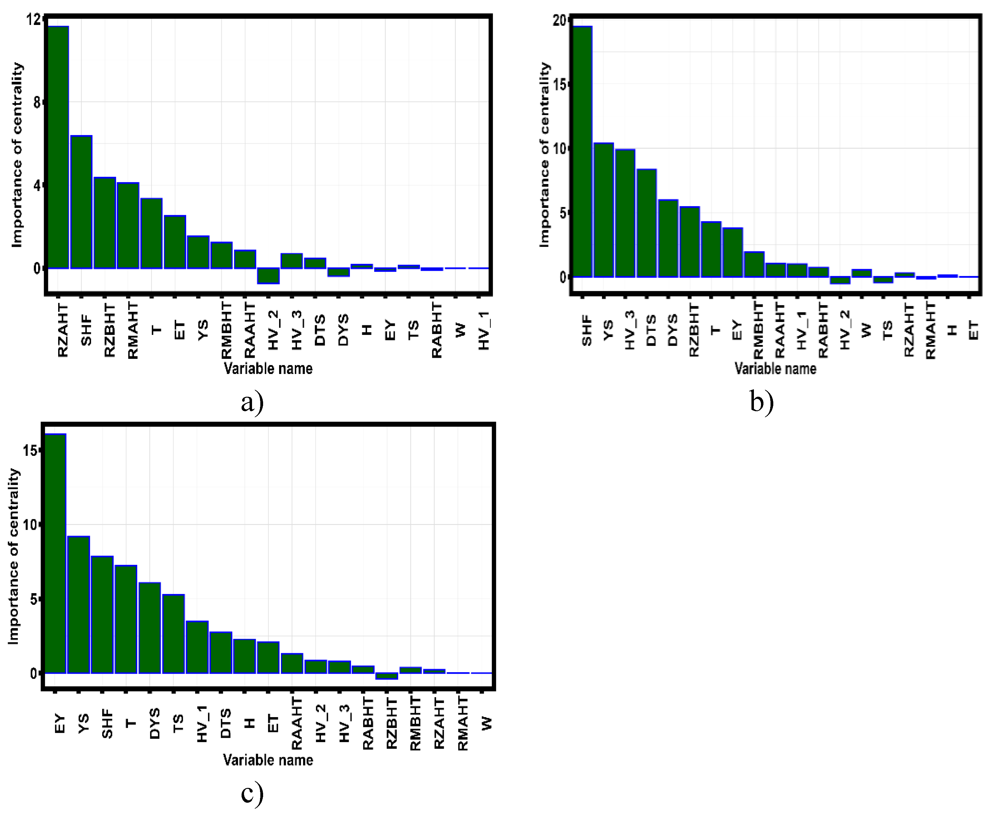
Centrality analysis carried out by equations (1)-(3) shows that when moving from group (1) to group (3), the parameter that gives the greatest contribution to the correlations between the variables present in the data set changes. In group 1, the most significant parameter is the Rz determined after heat treatment, in group 2 the strain hardening coefficient, and in group 3 the Young’s modulus. In group 1, the actual specimen width and HV_1 have zero relationships. In group 2, there are no variables with no relationships. In group 3, the actual width of the specimen does not have any linkage.
Figure 13 shows Tukey diagrams for the newly identified data groups for microhardness, strain hardening factor, Young’s modulus and Rz parameter after heat treatment (the groups are ordered according to the increase of the prevailing heat treatment temperatures in the intervals).
Figure 13.
- Behavior of central parameters selected based on correlation graph analysis in selected groups: a) Change of hardness (HV); b) Change of strain hardening coefficient; c) Change of Rz after heat treatment; d) Change of Young’s modulus (EY).
Figure 13.
- Behavior of central parameters selected based on correlation graph analysis in selected groups: a) Change of hardness (HV); b) Change of strain hardening coefficient; c) Change of Rz after heat treatment; d) Change of Young’s modulus (EY).
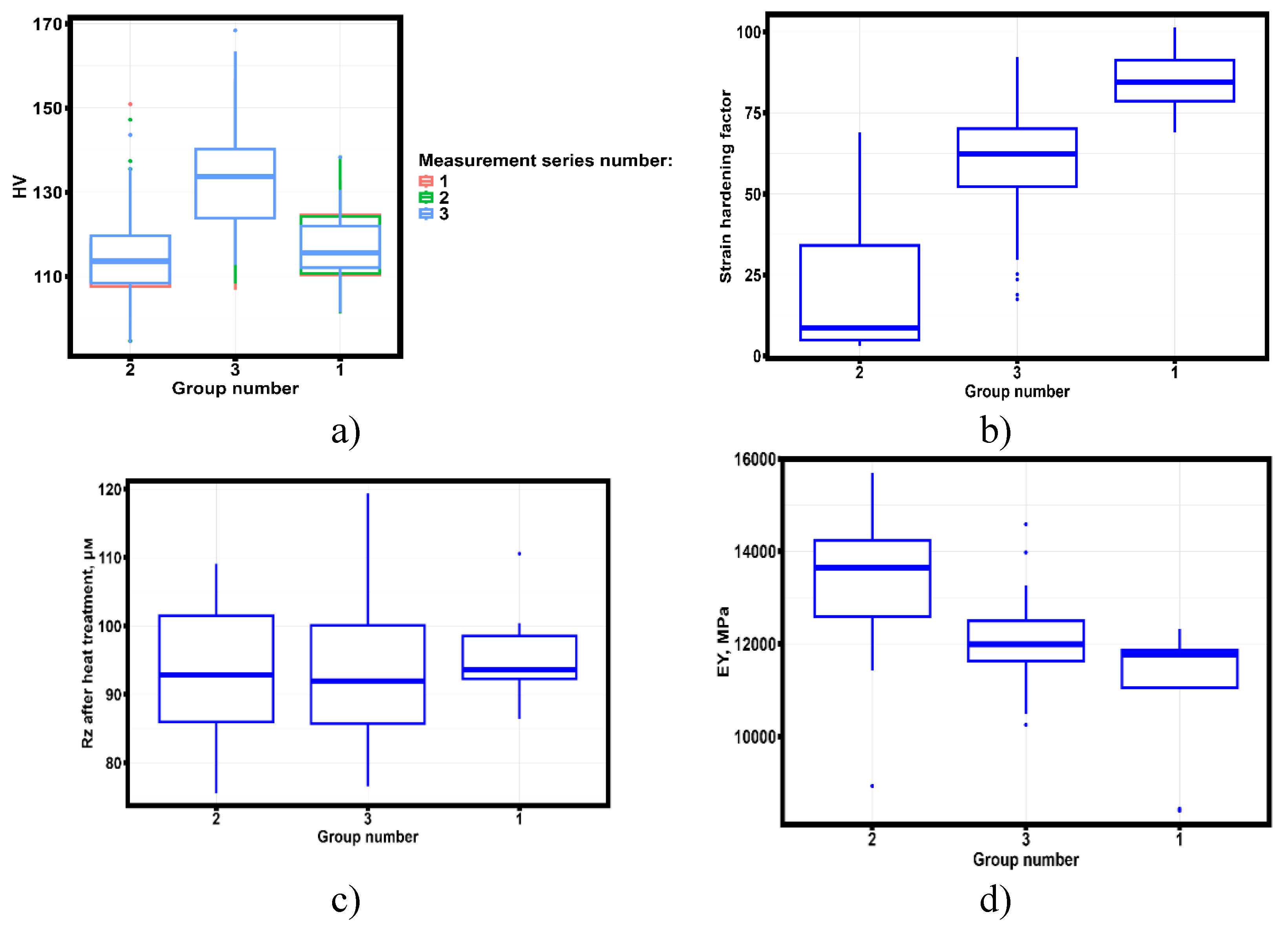
According to the results of the analysis, it can be assumed that the correlation between microhardness and surface roughness parameters is an intermediate link (Figure 12 A) linking strain hardening and elastic properties of studied samples. The analysis of statistical significance differences in the selected groups shows that the parameter Rz after heat treatment has no statistically significant differences, Young’s modulus is statistically significantly different in group 2 from group 3 and group 1 (p-value<0.05) and does not differ in group 3 and group 1 (p-value >0.05). The behavior of microhardness and strain hardening coefficient are statistically significantly different in all three groups (p-value<0.05). Based on the results of the analysis, we can construct explanatory robust regression equations linking the constant value of Rz after heat treatment with microhardness, strain hardening coefficient and Young’s modulus. The same equations can be obtained for the relationship between microhardness, Young’s modulus, strain hardening coefficient and heat treatment temperature. Robust regression equations linking the parameters having non-zero centrality determined by equations (1)-(3) and the parameter having the maximum number of links. In computing the robust regression equations, normalization [68,69,70] of the data was performed to allow comparison of the contributions of the variables to the explanation of the central variable. The robust regression equation in group 1 is as follows:
where T - heat treatment temperature; H - actual specimen thickness; W - actual specimen width; EY - Young’s modulus; ET - secant modulus; YS - yield strength; TS - tensile strength; RABHT - Ra before heat treatment; RZBHT - Rz before heat treatment; RMBHT - Rmax before heat treatment; RAAHT - Ra after heat treatment; RZAHT - Rz after heat treatment; RMAHT - Rmax after heat treatment; HV_1, HV_2 and HV_3 - Vickers microhardness in the first, second and third series of measurements; DTS - strain corresponding to the strength limit; DYS - strain corresponding to the yield limit; SHF - strain hardening factor.
The robust regression equation describing the relationship between the strain hardening coefficient and the rest of the parameters studied in group 2 is as follows:
where T - heat treatment temperature; H - actual specimen thickness; W - actual specimen width; EY - Young’s modulus; ET - secant modulus; YS - yield strength; TS - tensile strength; RABHT - Ra before heat treatment; RZBHT - Rz before heat treatment; RMBHT - Rmax before heat treatment; RAAHT - Ra after heat treatment; RZAHT - Rz after heat treatment; RMAHT - Rmax after heat treatment; HV_1, HV_2 and HV_3 - Vickers microhardness in the first, second and third series of measurements; DTS - strain corresponding to the strength limit; DYS - strain corresponding to the yield limit; SHF - strain hardening factor.
The robust regression equation describing the relationship between the strain hardening coefficient and the rest of the parameters studied in group 3 is as follows:
where T - heat treatment temperature; H - actual specimen thickness; W - actual specimen width; EY - Young’s modulus; ET - secant modulus; YS - yield strength; TS - tensile strength; RABHT - Ra before heat treatment; RZBHT - Rz before heat treatment; RMBHT - Rmax before heat treatment; RAAHT - Ra after heat treatment; RZAHT - Rz after heat treatment; RMAHT - Rmax after heat treatment; HV_1, HV_2 and HV_3 - Vickers microhardness in the first, second and third series of measurements; DTS - strain corresponding to the strength limit; DYS - strain corresponding to the yield limit; SHF - strain hardening factor.
Figure 14 shows the contributions of the variables under study to the accuracy losses of the models described by equations (8)-(10).
Figure 14.
- Evaluation of the influence of explanatory variables on the control parameter in three groups of samples obtained by selective laser melting technique from Al-Mn-Mg-Ti-Zr alloy.
Figure 14.
- Evaluation of the influence of explanatory variables on the control parameter in three groups of samples obtained by selective laser melting technique from Al-Mn-Mg-Ti-Zr alloy.

The analysis of the influence of explanatory variables on the control parameter shows that in group 1 the average surface roughness before heat treatment and the maximum surface roughness before heat treatment have the greatest influence. Whereas the mechanical properties of thin-walled specimens contribute less to explaining the error of equation (8) of which Young’s modulus is the most significant. In group 2 (equation 9), Young’s modulus, tensile strength and strain corresponding to the tensile strength are the most significant contributors in explaining the strain hardening factor. In group 3 (Equation 10), Young’s modules, secant modules, tensile strength and strain-hardening ratio make the largest contribution to the explanation of Young’s modules. For the most significant parameters (except for the average and maximum surface roughness before heat treatment and after heat treatment) empirical equations of robust regression were constructed describing the dependence of the most significant parameters on the heat treatment temperature with confidence intervals determined by bootstrapping methods. The estimation of the best approximation was carried out by the minimum Akaike criterion; polynomials of the first, second and third degree were considered as approximations.
Table 7 shows the dependences of the main parameters on the heat treatment temperature.
Table 8 presents the confidence intervals of the robust regression coefficients of the robust regression equations (11)-(15).
3.3. Monte Carlo statistical modeling
Table 3 presents the results of the evaluation of the closest distribution law of the experimental data by the Akaike and Bayesian information criteria, from which it follows that seven of the eight considered distribution laws are found in the experimental data. To confirm the established closest type of distribution, we evaluated the closeness of seven theoretical laws of distribution to the actual distribution, the results are presented in Figure 14.
Figure 14.
- Comparison of theoretical distribution laws with actual distribution laws of experimental data. A) PDF of Young’s modulus; B) PDF of secant modulus; C) PDF of ultimate strength; D) PDF of strain corresponding to ultimate strength; E) PDF of strain hardening coefficient.
Figure 14.
- Comparison of theoretical distribution laws with actual distribution laws of experimental data. A) PDF of Young’s modulus; B) PDF of secant modulus; C) PDF of ultimate strength; D) PDF of strain corresponding to ultimate strength; E) PDF of strain hardening coefficient.
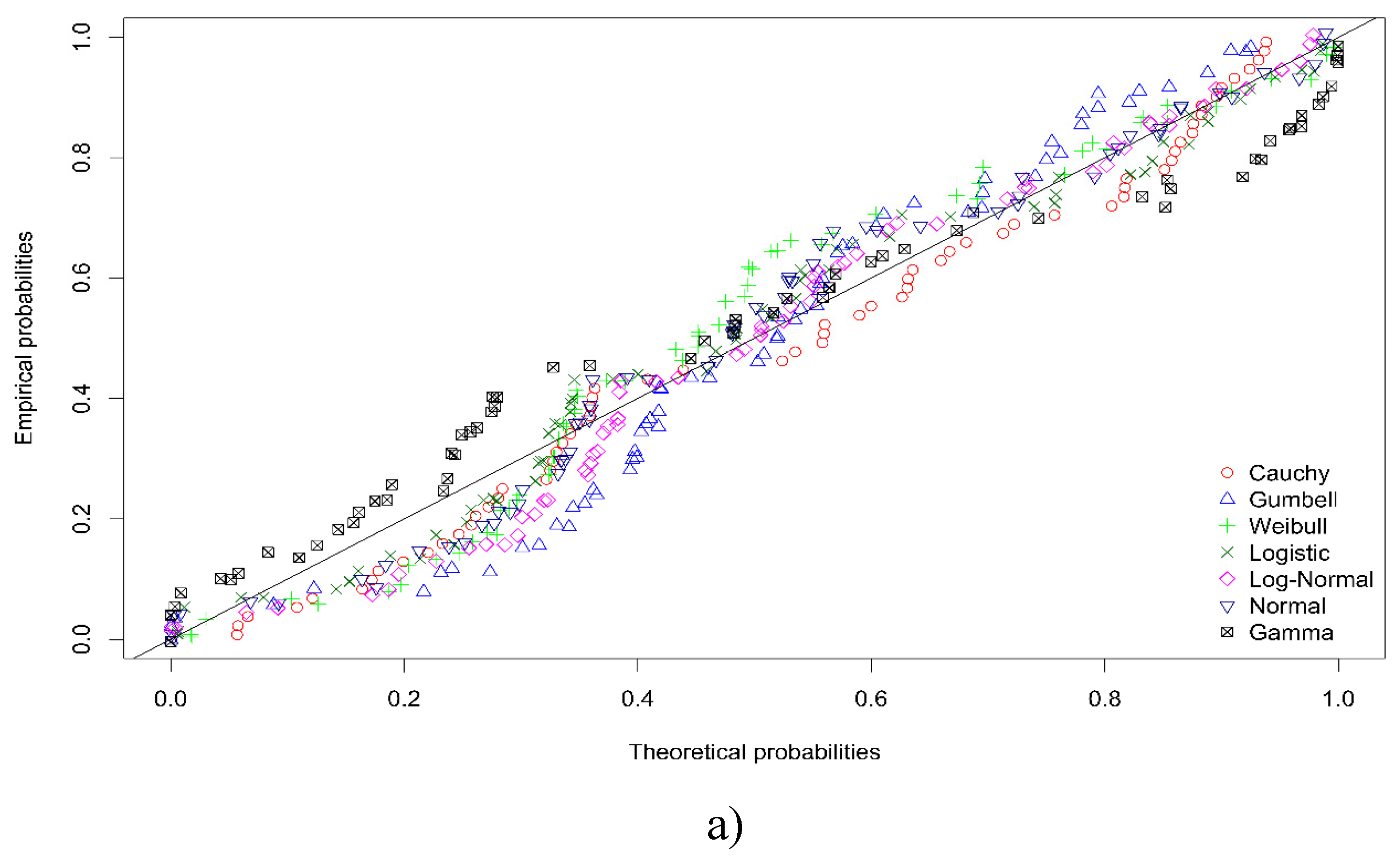
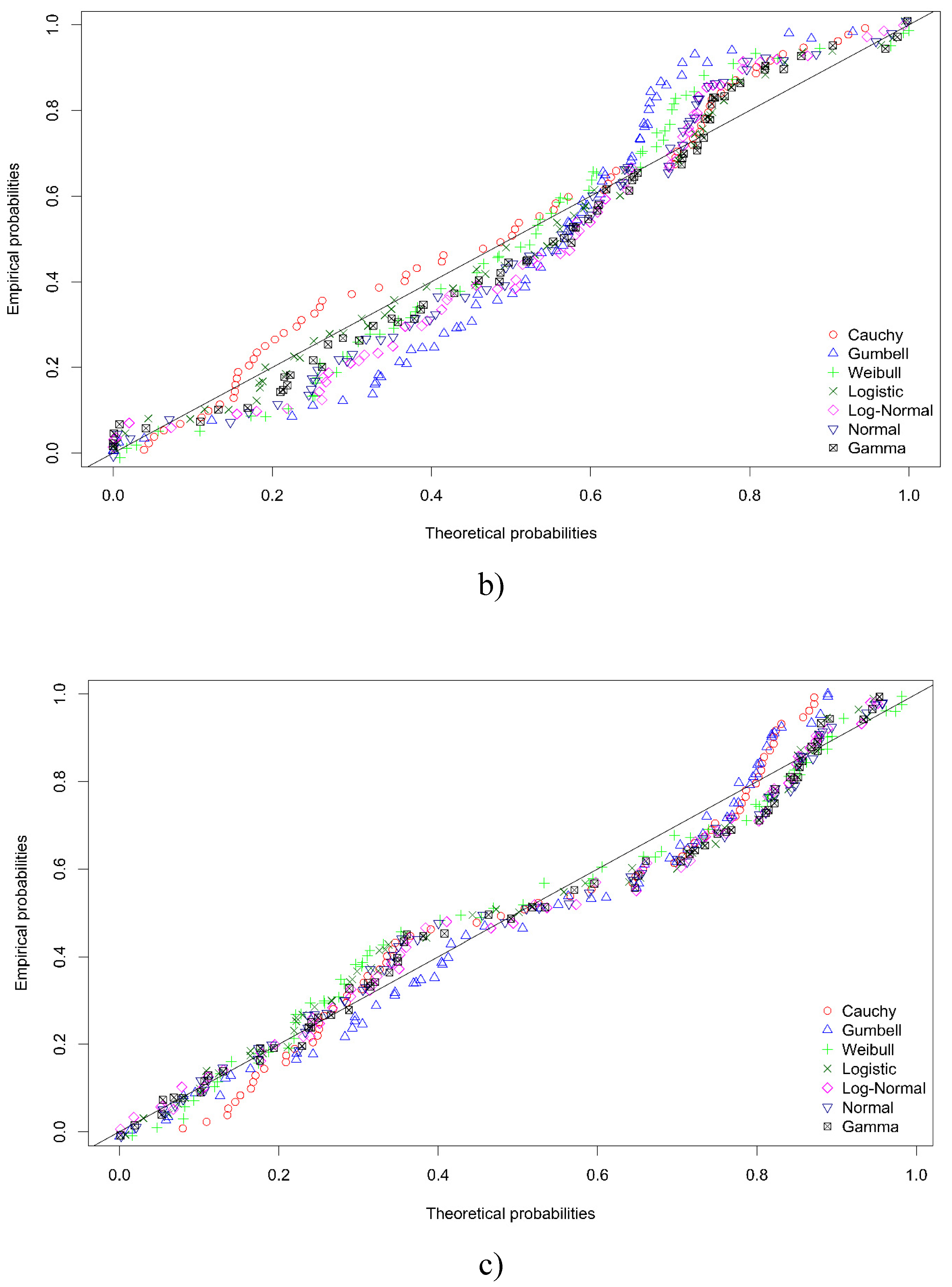
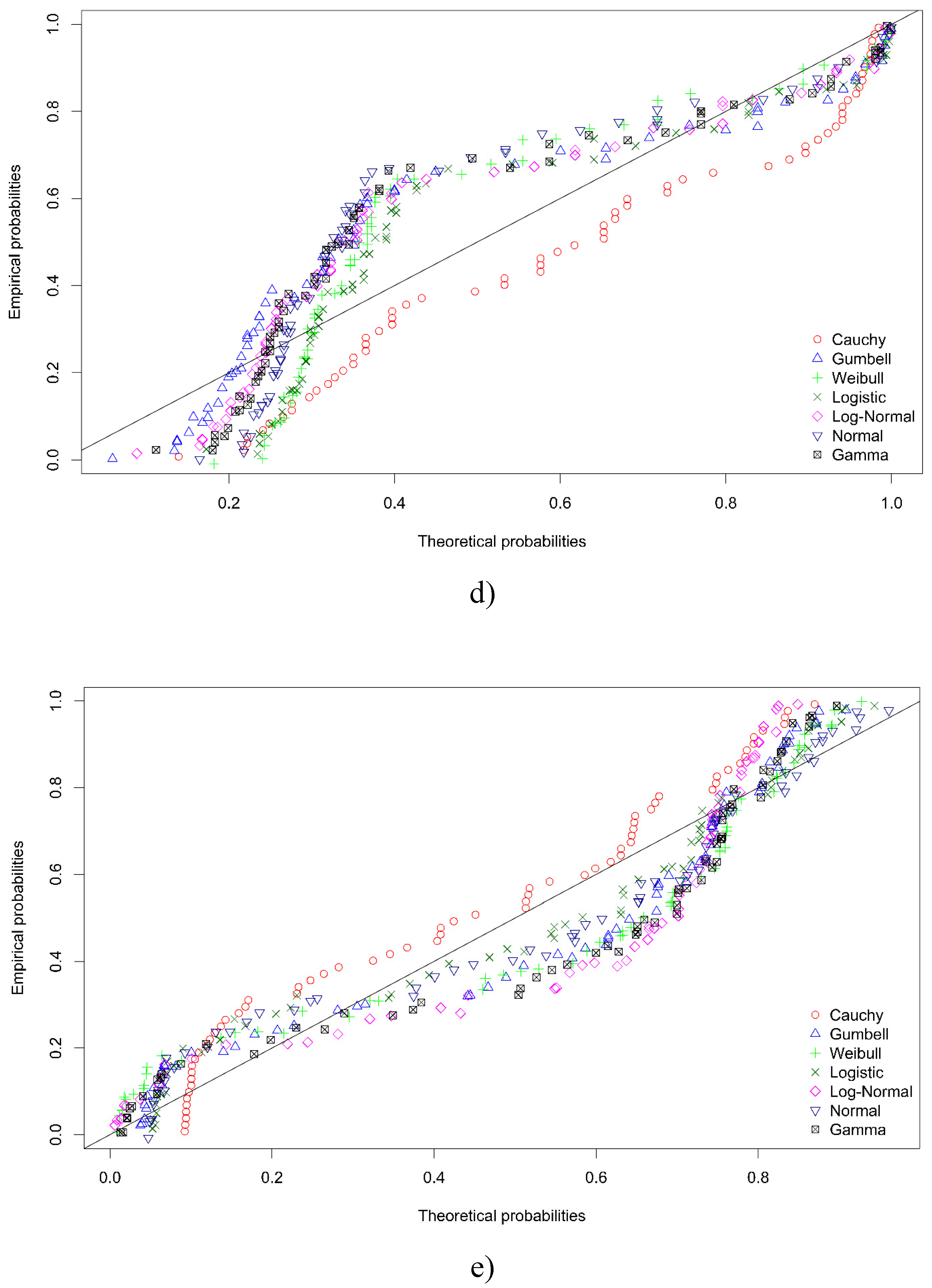
Table 9 presents the root mean square error between the theoretical and experimental likelihood function.
Comparison of the results of estimation of the mean square deviation of the theoretical distributions from the empirical distributions and the estimations carried out according to the Akaike and Bayesian information criteria coincide for Young’s modulus and secant modulus. Whereas, for the ultimate strength, strain corresponding to the ultimate strength and strain hardening coefficient, the distributions occupying the second place after the distribution laws having the minimum values of the information criteria are the closest. In accordance with recommendations [72,73,74], the distribution laws established based on PDF analysis and bound from above and below by equations (11)-(15) will be used for Monte Carlo simulation. Table 10 presents the robust regression equations approximating the change in the distribution coefficients as a function of the heat treatment temperature of the samples obtained by selective laser melting technology from Al-Mn-Mg-Ti-Zr alloy.
Figure 15 shows a histogram of the distribution of new annealing temperatures generated from the uniform distribution.
Figure 16 shows plots of dependence on the values predicted by equations (11)-(15) for annealing temperatures generated according to the uniform distribution law from the sample obtained by the Monte Carlo method and a histogram of the scatter of residuals between the model data and the results of prediction by equations (11)-(15).
Figure 17 shows the dependence of data obtained because of Monte Carlo simulation on the values obtained because of tensile tests of thin-walled samples obtained by selective laser melting technology from Al-Mn-Mg-Ti-Zr alloy.
Figure 17.
- Dependence of experimental values of the most significant quantities selected based on the analysis of robust regression equations (8)-(10) on the values obtained by Monte Carlo method. a) Scatter diagram of the predicted values of Young’s modulus; b) Histogram of the distribution of the residuals of the difference of two models; c) Scatter diagram of the predicted values of modulus along the secant; d) Histogram of the distribution of the residuals of the difference of models; e) Scatter diagram of the predicted values of ultimate strength; f) Histogram of the distribution of residuals; g) Scatter diagram of the predicted values of strain hardening coefficient; h) Histogram of the distribution of residuals of models; i) Scatter diagram of the predicted values of strain corresponds to the values of the strain hardening coefficient; j) Histogram of the distribution of residuals of models;.
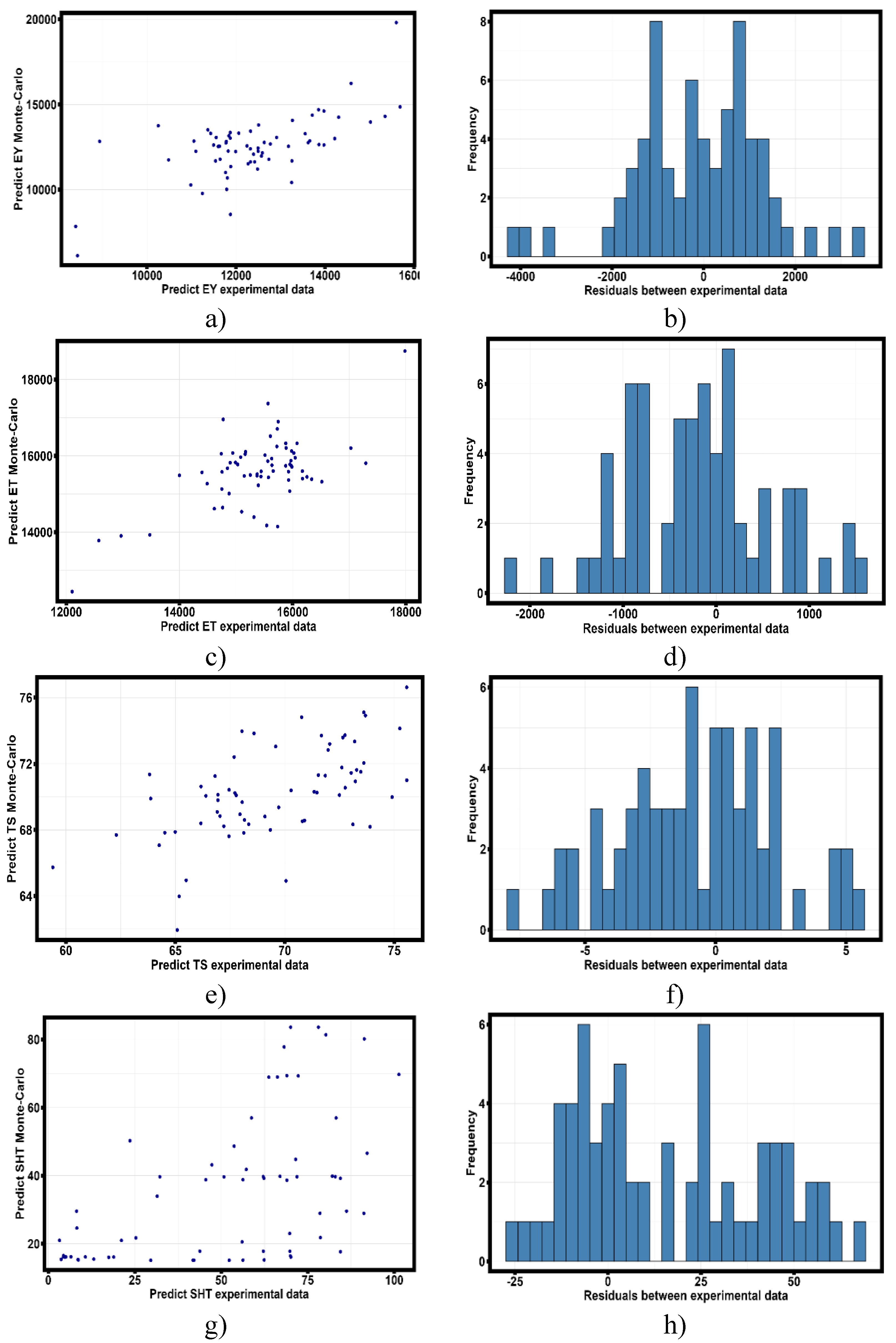
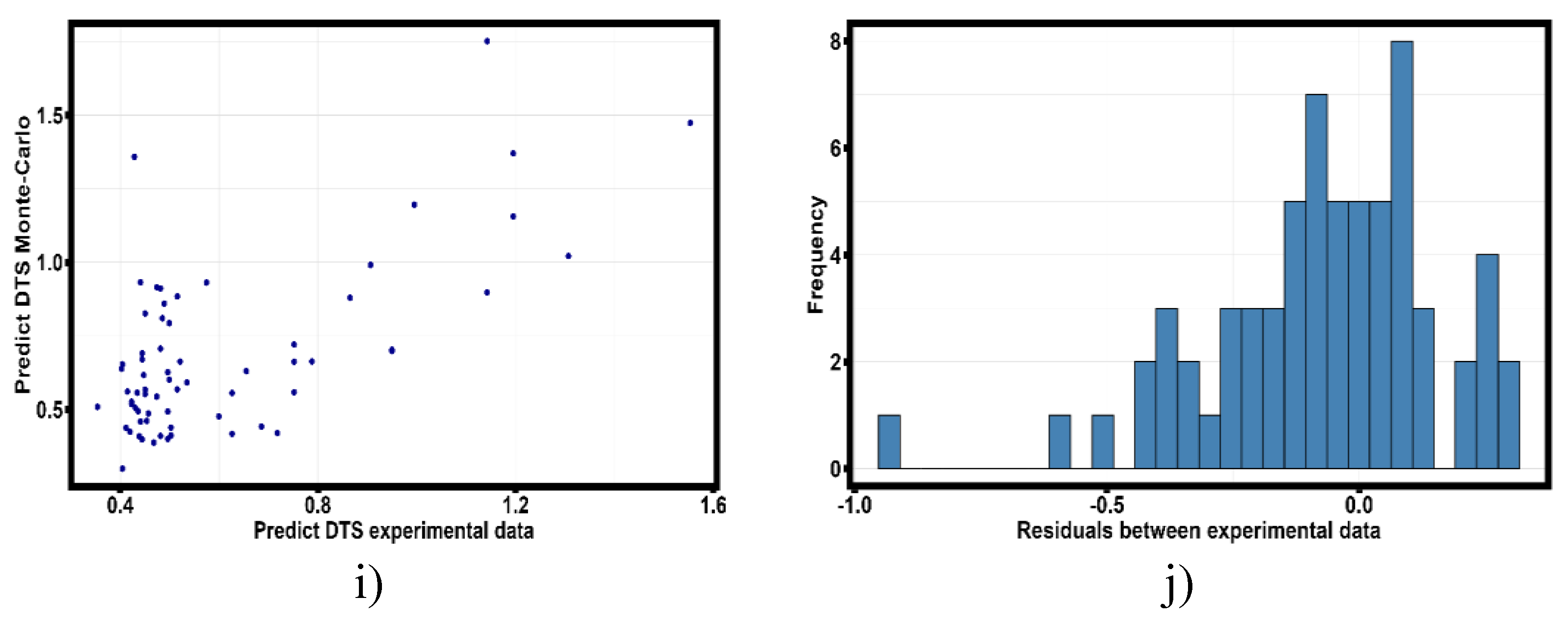
Evaluation of linear dependence between experimentally obtained results, robust regression models and results predicted by Monte Carlo method is presented in Table 12. The estimation was carried out by Pearson correlation coefficient.
The results of correlation analysis show that the model based on the Monte Carlo method agrees better with the experimental data than the empirical model based on robust regression. Provided that the validation heat treatment temperature obeys a uniform distribution law. The exception is the prediction of the strain hardening coefficient, the robust regression equation describes the strain hardening coefficient more accurately, which may be the subject of refinement of the empirical Monte Carlo model.
3.4. Discussion
Statistical analysis of the results of tensile tests of specimens made by selective laser melting technology from Al-Mn-Mg-Ti-Zr alloy and subjected to heat treatment at temperatures from 260 ºC to 530 ºC within an hour showed that at temperatures of heat treatment from 20 ºC to 290 ºC the parameter having the largest number of statistically significant relationships is the strain hardening coefficient (Figure 13 B). At the same time, the analysis of the dependence of the strain hardening coefficient on the heat treatment temperature shows continuous growth with increasing temperature. Such behavior of the investigated value may indicate different mechanisms of strain hardening of samples subjected to heat treatment at temperatures from 260 ºC to 530 ºC. To identify the reasons for the growth of strain hardening coefficient, metallographic and X-ray phase analysis of thin-walled samples obtained by selective laser melting technology was carried out. Figure 17 shows the results of metallographic analysis of thin-walled samples subjected to heat treatment at different temperatures.
Figure 17.
- Optic (left column) and SEM (right column) images of thin-walled samples fabricated by selective laser melting of Al-Mn-Mg-Ti-Zr alloy. A), B) Without heat treatment; C), D) Heat treatment at 290 °C; E), F) Heat treatment at 320 °C; G), H) Heat treatment at 410 °C; I), J) Heat treatment at 470 °C; K), L) Heat treatment at 530 °C.
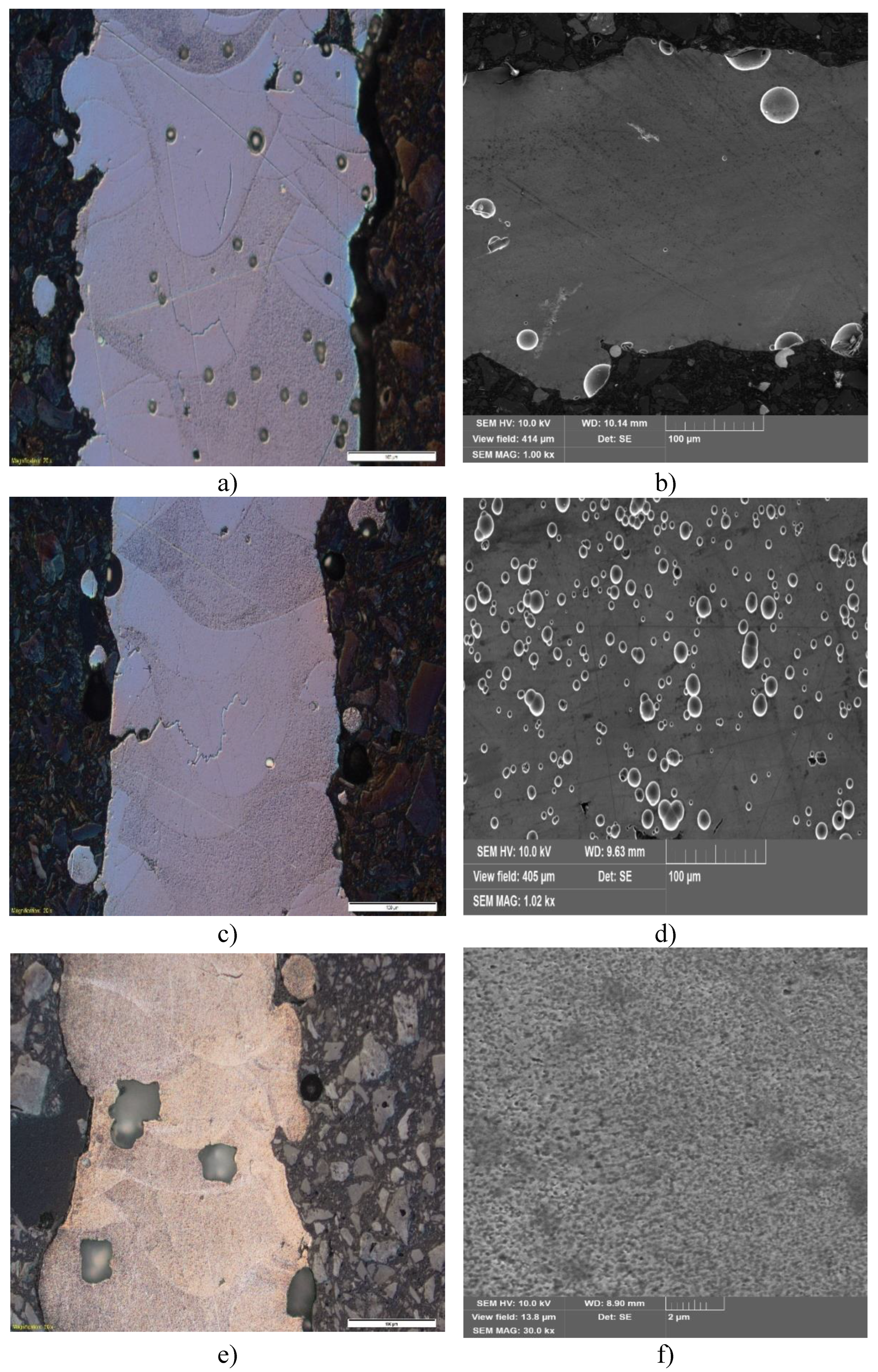
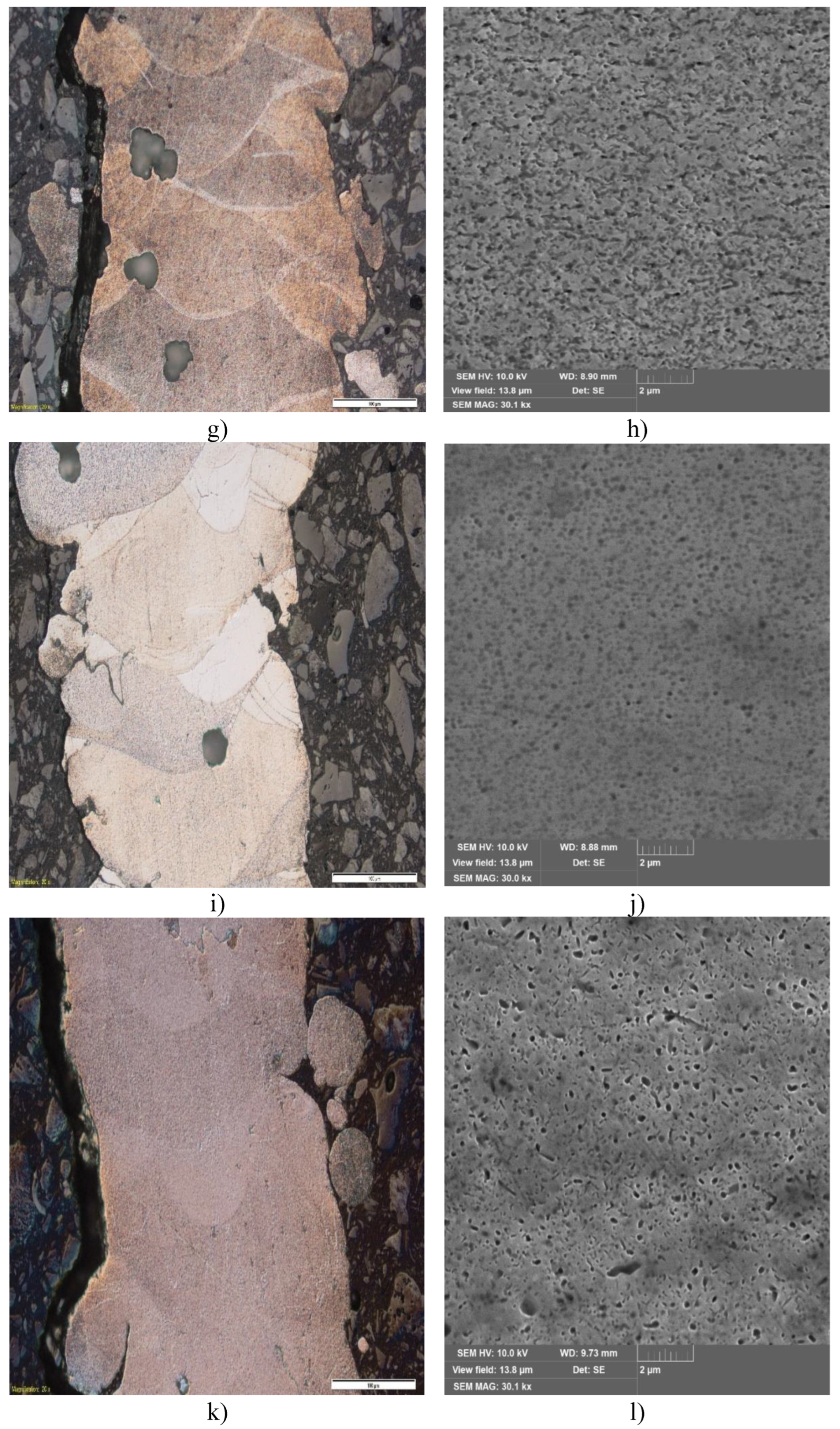
The analysis of presented images shows that the number of macropores and microcracks in the samples decreases with increasing heat treatment (Figure 17 A, D). After the temperature of 290 ºC (Figure 17 D, E) there are agglomerations (dark inclusions) at the melt bath boundaries and there are no macropores, but there are micropores. Comparing the results of metallographic analysis with the results of statistical analysis, the samples without heat treatment and heat treated at 260 ºC and 290 ºC fell into the same group (group 2 Table 6) and had the most significant mechanical property - strain hardening coefficient. It was shown on model specimens [30] that the strain hardening coefficient increases almost twofold when the size of macrodefects decreases. Accordingly, the increase in strain hardening coefficient observed in Figure 13b can be explained through the mechanism of macrodefect reduction. This conclusion is confirmed, among other things, by the results of X-ray phase analysis.
Figure 18 shows the results of XRD analysis corresponding to the samples without and with heat treated and at 290 ºC for one hour.
Changes in the intensity of the peaks observed in the X-ray diagram (Figure 18) are associated with an increase in the concentration of manganese precipitating from the solid solution of aluminum and forming a compound with oxygen.
At higher heat treatment temperatures, in addition to the concentration of defects at the van-melt boundaries, the formation of light (white) zones at the van-melt boundary is observed (Figure 19 D and G). The formation of these areas is associated with intensive precipitation of manganese and magnesium with subsequent formation of oxides. Figure 20 shows the X-ray diffraction pattern of sample heat-treated at 410 ºC and 470 ºC.
The statistical analysis shows that for the samples in group 3, the parameter with the largest number of statistically significant correlations is Young’s modulus, and in second place is the strain hardening coefficient (Figure 13 C). That in combination with the results presented in Figure 17 indicates that the precipitation of manganese and magnesium oxides on the melt bath boundaries reduce the elastic properties of the samples and to a lesser extent (than the reduction of macro-defectivity) contributes to the increase in the strain hardening coefficient.
Further increase in the temperature of heat treatment of thin-walled samples obtained by selective laser melting technology leads to the precipitation of pure titanium with hexagonal crystallographic structure from the solid solution and the formation of intermetallic phase Mg8Al16 and further decrease in the level of macrodefectivity. Figure 21 shows the X-ray radiography of sample heat-treated at 530 ºC for 1 hour.
Statistical analysis of the results showed that for specimens in the first group, the greatest number of statistically significant correlations is observed for the sum of heights of the largest protrusions and depths of the largest depressions of the surface roughness profile within the base length of the specimen (Rz) given by Eq:
where – height of i-th protrusion of surface roughness profile; – depth of the i-th depression of the surface roughness profile.
Why is the highest statistically significant correlation achieved after heat treatment at 530 ºC between the parameter Rz and microhardness (Figure 11 A). Simultaneously with this fact, microstructural analysis shows the presence of a more homogeneous structure with a small number of micropores, and the results of XRD analysis show that the formation of intermetallic phases and the precipitation of titanium and zirconium from the solid solution. It follows that micropores formed because of selective laser melting during high-temperature heat treatment are shifted to the melt bath boundary with subsequent exit to the sample surface.
Analysis of microhardness behavior (Figure 13 a) shows that group 2 with low heat treatment temperature has the lowest microhardness for the three series of measurements. But the change of sign of the robust regression coefficient (Equation 9) at different series of microhardness measurements shows that each series of measurements falls into different phases contributing positively or negatively to the explanation of the strain hardening coefficient. However, these differences are not statistically significant, which suggests that the distribution of phases is not large and uniform around indenter penetration during measurements. A similar situation is observed in group three, considering the results (Figure 13 a), it can be stated that the amount of microhardness increasing phase increases and the sign of the contribution to the explanation of Young’s modulus (Equation 10) does not change (Equation 9). The decrease in microhardness of samples in group 1 and the change in the contribution of the measurement series (Equation 8) shows that the microstructure of the samples undergoes significant changes compared to group 2 and 3.
The cumulative analysis of the results of the conducted studies shows that at increasing the temperature of heat treatment micropores (macrodefects) are shifted to the boundary of the melt zones with subsequent exit to the surface, which together with the formation of intermetallic phase and the release of titanium and zirconium leads to strain hardening of thin-walled samples obtained by selective laser melting of Al-Mn-Mg-Ti-Zr alloy.
The analysis of the results of modeling the variables contributing the main contribution to the prediction error of the parameters having the maximum number of correlations (equations 8-10) shows that in most cases the semi-empirical model based on the Monte Carlo method and Latin Hypercube more accurately describes the experimental data compared to the robust regression model (equations (11)-(15)). The exception is the behavior of the strain hardening coefficient (Table 12). During the modeling process, it was found that increasing the number of simulated specimens to 100 increases the Pearson correlation coefficient to 0.93. Thus, further research in the construction of a semi-empirical Monte Carlo model will be aimed at harmonizing the volume of experimental and generated samples to improve the accuracy of the model.
4. Conclusion
The statistical and experimental studies of mechanical properties and surface roughness of thin-walled samples obtained by selective laser melting technology from Al-Mn-Mg-Ti-Zr alloy and subjected to heat treatment at temperatures from 260 ºC to 530 ºC demonstrate:
- Heat treatment of thin-walled specimens made of Al-Mn-Mg-Ti-Zr alloy at temperatures of 530 ºC for one hour allows to significantly reduce the level of macro-defectivity and obtain maximum strain hardening in comparison with hardening at lower temperatures of heat treatment.
- The main contribution to strain hardening of thin-walled samples produced by selective laser melting technology is due to the reduction of macro-defectivity. The secondary cause is perceptual hardening due to the precipitation of manganese, magnesium, titanium and zirconium from the solid solution and disperse hardening due to the formation of intermetallic phase Mg8Al16.
- Decrease in the level of macrodefectivity occurs due to the movement of micropores to the melt bath boundary with subsequent exit to the surface of the sample. The smallest number of defects and microcracks is observed in samples heat-treated at 530 ºC for one hour.
- The analysis of changes in the contributions of series of microhardness measurements shows that the maximum hardness is achieved at heat treatment temperatures from 320 ºC to 500 ºC. Whereas at 530 ºC the microhardness of the samples decreases, which is explained by significant changes in the structural phase composition.
- Validation of the developed robust regression and semi-empirical Monte Carlo models shows that the Monte Carlo-based model more accurately explains the most significant mechanical properties, except for the strain hardening coefficient.
Further studies will be aimed at identifying the mechanism of micropore movement to the melt bath boundary and refining Monte Carlo models considering other parameters that influence the formation of the sample structure.
Author Contributions
Conceptualization, N.Y.N.; methodology, N.Y.N.; software, P.P., A.S.; validation, R.S.K., N.W.S.P., I. I.; formal analysis, N.Y.N.; investigation, R.S.K., P.P., A.S.; resources, I. I., R.S.K.; data curation, N.Y.N.; writing—original draft preparation N.Y.N.; writing—review and editing N.Y.N., N.W.S.P., A.S.; visualization, P.P., N.W.S.P.; supervision, N.Y.N., S.N.G.; project administration, T.V.T., S.N.G.; funding acquisition, T.V.T. All authors have read and agreed to the published version of the manuscript.
Funding source
The research was financially supported by the Ministry of Science and Higher Education of the Russian Federation (project No. FSFS-2024-0024).
Data Availability Statement
All data are presented in the publication.
Acknowledgments
Not applicable.
Conflicts of Interest
The authors declare no conflict of interest.
Application A:
File with data set: Data.csv
File describing the dataset: ReadmeData.txt
Application B:
File with basic statistics results: BaseStat.csv
File describing the basic statistics results: ReadmeBS.txt
References
- International Organization for Standardization. ISO/ASTM 52900:2015 [ASTM F2792] Additive Manufacturing-General Principles-Terminology; ISO: Geneva, Switzerland, 2015.
- Ian Gibson, David Rosen, Brent Stucker. Additive Manufacturing Tecnologies. 3D Printing, Rapid Prototyping and Direct Digital Manufacturing//Springer, 2015 – P.P. 648.
- Borgue, R. 3D printing: the dawn of a new era in manufacturing? / R. Borgue // Assembly Automation. 2013. Vol. 33. ¹4. P. 307-311.
- S.A.M. Tofail, E.P. Koumoulos, A. Bandyopadhyay, S. Bose, L. O’Donoghue, C. Charitidis, Additive manufacturing: scientific and technological challenges, market uptake and opportunities, Mater. Today 21 (2018) 22e37. [CrossRef]
- J.M. Lee, S.L. Sing, M.M. Zhou, W.Y. Yeong, 3D bioprinting processes: a perspective on classification and terminology, Int. J. Bioprint. 4 (2) (2018) 151. [CrossRef]
- T. DebRoy, H.L. Wei, J.S. Zuback, T. Mukherjee, J.W. Elmer, J.O. Milewski, A.M. Beese, A. Wilson-Heid, A. De, W. Zhang, Additive manufacturing of metallic componentseprocess, structure and properties, Prog. Mater. Sci. 92 (2018) 112e224.
- J. Haubrich, J. Gussone, P. Barriobero-Vila, P. Kürnsteiner, E.A. Jagle, D. Raabe, € N. Schell, G. Requena, The role of lattice defects, element partitioning and intrinsic heat effects on the microstructure in selective laser melted Ti-6Al-4V, Acta Mater. 167 (2019) 136e148.
- Tian, Qiwen. “The development status of selective laser melting technology (SLM).” Journal of Physics: Conference Series. Vol. 1798. No. 1. IOP Publishing, 2021.
- Kaufman, John Gilbert, ed. Properties of aluminum alloys: tensile, creep, and fatigue data at high and low temperatures. ASM international, 1999.
- Polmear, I. J., and M. J. Couper. “Design and development of an experimental wrought aluminum alloy for use at elevated temperatures.” Metallurgical transactions A 19 (1988): 1027-1035. [CrossRef]
- Wang, G. S., K. Liu, and S. L. Wang. “Evolution of elevated-temperature strength and creep resistance during multi-step heat treatments in Al-Mn-Mg alloy.” Materials 11.7 (2018): 1158. [CrossRef]
- Van Dalen, Marsha E., et al. “Effects of Yb and Zr microalloying additions on the microstructure and mechanical properties of dilute Al–Sc alloys.” Acta Materialia 59.20 (2011): 7615-7626.
- Lai, J., Z. Zhang, and X-G. Chen. “The thermal stability of mechanical properties of Al–B4C composites alloyed with Sc and Zr at elevated temperatures.” Materials Science and Engineering: A 532 (2012): 462-470. [CrossRef]
- Farkoosh, A. R., X. Grant Chen, and M. Pekguleryuz. “Dispersoid strengthening of a high temperature Al–Si–Cu–Mg alloy via Mo addition.” Materials Science and Engineering: A 620 (2015): 181-189.
- Liu, Kun, Hezhaoye Ma, and X-Grant Chen. “Enhanced elevated-temperature properties via Mo addition in Al-Mn-Mg 3004 alloy.” Journal of alloys and compounds 694 (2017): 354-365. [CrossRef]
- Mikhaylovskaya, A. V., et al. “Effect of homogenisation treatment on precipitation, recrystallisation and properties of Al–3% Mg–TM alloys (TM= Mn, Cr, Zr).” Materials & Design 109 (2016): 197-208.
- Engler, Olaf, Zhenshan Liu, and Katrin Kuhnke. “Impact of homogenization on particles in the Al–Mg–Mn alloy AA 5454–Experiment and simulation.” Journal of Alloys and Compounds 560 (2013): 111-122.
- Radetić, Tamara, Miljana Popović, and Endre Romhanji. “Microstructure evolution of a modified AA5083 aluminum alloy during a multistage homogenization treatment.” Materials characterization 65 (2012): 16-27. [CrossRef]
- Engler, Olaf, and Simon Miller-Jupp. “Control of second-phase particles in the Al-Mg-Mn alloy AA 5083.” Journal of Alloys and Compounds 689 (2016): 998-1010. [CrossRef]
- Engler, Olaf, Katrin Kuhnke, and Jochen Hasenclever. “Development of intermetallic particles during solidification and homogenization of two AA 5xxx series Al-Mg alloys with different Mg contents.” Journal of Alloys and Compounds 728 (2017): 669-681. [CrossRef]
- Cadek, Josef. “Creep in precipitation- and dispersion-strengthened alloys(a review).” MET MATER(CAMBRIDGE ENGL). 29.6 (1991): 385-398.
- Knipling, Keith E., David C. Dunand, and David N. Seidman. “Criteria for developing castable, creep-resistant aluminum-based alloys–A review.” International Journal of Materials Research 97.3 (2022): 246-265.
- Zhu, Ai Wu, et al. “The intelligent design of high strength, creep-resistant aluminum alloys.” Materials Science Forum. Vol. 396. Trans Tech Publications Ltd, 2002. [CrossRef]
- Knipling, Keith E., and David C. Dunand. “Creep resistance of cast and aged Al–0.1 Zr and Al–0.1 Zr–0.1 Ti (at.%) alloys at 300–400 C.” Scripta Materialia 59.4 (2008): 387-390.
- Krug, Matthew E., and David C. Dunand. “Modeling the creep threshold stress due to climb of a dislocation in the stress field of a misfitting precipitate.” Acta Materialia 59.13 (2011): 5125-5134. [CrossRef]
- Marquis, Emmanuelle A., and David C. Dunand. “Model for creep threshold stress in precipitation-strengthened alloys with coherent particles.” Scripta Materialia 47.8 (2002): 503-508. [CrossRef]
- Kittel, Charles, and Paul McEuen. Introduction to solid state physics. John Wiley & Sons, 2018.
- Yu. A. Abuzin, N. Yu. Nikitin. Determination of promising areas of research in the field of aluminum-based alloys using the electronic theory of metals // Non-Ferrous Metals. - 2012. - № 4. - С. 74-77.
- Nikitin, N. Y. A first-principles investigation of the effect of relaxation on the alloy formation in the aluminum-3d-transition-metal system / N. Y. Nikitin // The Physics of Metals and Metallography. – 2012. – Vol. 113, No. 5. – P. 427-437. 1134. [CrossRef]
- Grigoriev, Sergey, et al. “Mechanical properties variation of samples fabricated by fused deposition additive manufacturing as a function of filler percentage and structure for different plastics.” Scientific Reports 14.1 (2024): 28344. [CrossRef]
- Zhang, Xing, et al. “Microstructure evolution during selective laser melting of metallic materials: A review.” Journal of Laser Applications 31.3 (2019). [CrossRef]
- Li, Ruidi, et al. “Densification behavior of gas and water atomized 316L stainless steel powder during selective laser melting.” Applied surface science 256.13 (2010): 4350-4356. [CrossRef]
- E.V. Shelekhov, T.A. Sviridova, Programs for X-rayanalysis of polycrystals, Metal Sci. Heat Treat. 42 (2000)309–313. [CrossRef]
- S. Grazulis, D. Chateigner, R.T. Downs, A.T. Yokochi, M.Quiros, L. Lutterotti, E. Manakova, J. Butkus, P. Moeck, A.Le Bail, Crystallography open database an open-accesscollection of crystal structures, J. Appl. Cryst. 42 (2009) 726–729. [CrossRef]
- Tukey, John W. Exploratory data analysis. Addison-Wesley Pub. Co., c1977. - xvi, 688 p.
- H. Akaike, in Applications of Statistics, edited by P. R. Krishnaiah North-Holland, Amsterdam, 1977, p. 27.
- Y. Sakamoto, M. Ishiguro, and G. Kitagawa, Akaike Information Criterion Statistics Reidel, Dordrecht, 1983.
- Neath, Andrew A., and Joseph E. Cavanaugh. “The Bayesian information criterion: background, derivation, and applications.” Wiley Interdisciplinary Reviews: Computational Statistics 4.2 (2012): 199-203.
- Schwarz, Gideon. “Estimating the dimension of a model.” The annals of statistics (1978): 461-464.
- Rossi, Richard J. Mathematical statistics: an introduction to likelihood based inference. John Wiley & Sons, 2018.
- Shapiro, S.S.; Wilk, M.B. An analysis of variance test for normality. Biom. Trust 1965, 52, 591–611.
- D’Agostino, Ralph B.; Pearson, E. S. (1973). “Tests for Departure from Normality. Empirical Results for the Distributions of b2 and √b1”. Biometrika. 60 (3): 613–622.
- Kolmogorov, A.N. Sulla determinazione empirica di une legge di distribuzione. G. Ist. Ital. Attuari 1933, 4, 83–91.
- W. Anderson, On the Distribution of the Two-Sample Cramer-von Mises Criterion// Ann. Math. Statist. 33(3): 1148-1159 (September, 1962).
- Robert, Christian P., George Casella, and George Casella. Monte Carlo statistical methods. Vol. 2. New York: Springer, 1999.
- de Araújo-Neto, Vitaliano Gomes, et al. “Evaluation of physico-mechanical properties and filler particles characterization of conventional, bulk-fill, and bioactive resin-based composites.” journal of the mechanical behavior of biomedical materials 115 (2021): 104288.
- Kruskal, William H., and W. Allen Wallis. “Use of ranks in one-criterion variance analysis.” Journal of the American statistical Association 47.260 (1952): 583-621.
- Dunnett, Charles W. “New tables for multiple comparisons with a control.” Biometrics 20.3 (1964): 482-491. [CrossRef]
- Bonferroni, C. E., Teoria statistica delle classi e calcolo delle probabilità, Pubblicazioni del R Istituto Superiore di Scienze Economiche e Commerciali di Firenze 1936.
- Nielsen, Frank. Introduction to HPC with MPI for Data Science. Springer, 2016. [CrossRef]
- Pearson, Karl. “VII. Note on regression and inheritance in the case of two parents.” proceedings of the royal society of London 58.347-352 (1895): 240-242.
- Spearman, Charles. “The proof and measurement of association between two things.” (1961).
- Evans, James D. Straightforward statistics for the behavioral sciences. Thomson Brooks/Cole Publishing Co, 1996.
- Nieminen, Juhani. “On the centrality in a graph.” Scandinavian journal of psychology 15.1 (1974): 332-336.
- Alvarez-Socorro, A. J., G. C. Herrera-Almarza, and L. A. González-Díaz. “Eigencentrality based on dissimilarity measures reveals central nodes in complex networks.” Scientific reports 5.1 (2015): 17095. [CrossRef]
- Pillai, S. Unnikrishna, Torsten Suel, and Seunghun Cha. “The Perron-Frobenius theorem: some of its applications.” IEEE Signal Processing Magazine 22.2 (2005): 62-75. [CrossRef]
- Huber P. J. Robust statistics. – John Wiley & Sons, 2004. – Т. 523.
- Massy, William F. “Principal components regression in exploratory statistical research.” Journal of the American Statistical Association 60.309 (1965): 234-256.
- Hotelling, Harold. “The relations of the newer multivariate statistical methods to factor analysis.” British Journal of Statistical Psychology 10.2 (1957): 69-79. [CrossRef]
- Vořechovský, Miroslav, and Drahomír Novák. “Correlation control in small-sample Monte Carlo type simulations I: A simulated annealing approach.” Probabilistic Engineering Mechanics 24.3 (2009): 452-462. [CrossRef]
- Vořechovský, M. “Correlation control in small sample Monte Carlo type simulations II: Analysis of estimation formulas, random correlation and perfect uncorrelatedness.” Probabilistic Engineering Mechanics 29 (2012): 105-120. [CrossRef]
- Ramachandran, B. Theory of Characteristic Functions, Statistical Publishing Society, Calcutta. (1967).
- Huntington, D. E., and C. S. Lyrintzis. “Improvements to and limitations of Latin hypercube sampling.” Probabilistic engineering mechanics 13.4 (1998): 245-253. [CrossRef]
- Olsson, Anders, Göran Sandberg, and Ola Dahlblom. “On Latin hypercube sampling for structural reliability analysis.” Structural safety 25.1 (2003): 47-68. [CrossRef]
- Patterson, H. D. “The errors of lattice sampling.” Journal of the Royal Statistical Society Series B: Statistical Methodology 16.1 (1954): 140-149.
- Keramat, Mansour, and Richard Kielbasa. “Efficient average quality index estimation of integrated circuits by modified Latin hypercube sampling Monte Carlo (MLHSMC).” 1997 IEEE International Symposium on Circuits and Systems (ISCAS). Vol. 3. IEEE, 1997.
- Huntington, D. E., and C. S. Lyrintzis. “Improvements to and limitations of Latin hypercube sampling.” Probabilistic engineering mechanics 13.4 (1998): 245-253. [CrossRef]
- van Laarhoven, Peter JM. “Theoretical and computational aspects of simulated annealing.” (1988).
- Ali, Peshawa Jamal Muhammad, et al. “Data normalization and standardization: a technical report.” Mach Learn Tech Rep 1.1 (2014): 1-6.
- Raju, VN Ganapathi, et al. “Study the influence of normalization/transformation process on the accuracy of supervised classification.” 2020 Third International Conference on Smart Systems and Inventive Technology (ICSSIT). IEEE, 2020.
- Trebuňa, Peter, et al. “The importance of normalization and standardization in the process of clustering.” 2014 IEEE 12th International Symposium on Applied Machine Intelligence and Informatics (SAMI). IEEE, 2014.
- Awad, Adnan M. “Properties of the Akaike information criterion.” Microelectronics Reliability 36.4 (1996): 457-464. [CrossRef]
- Chen, Xiaoming. “Using Akaike information criterion for selecting the field distribution in a reverberation chamber.” IEEE transactions on electromagnetic compatibility 55.4 (2012): 664-670. [CrossRef]
- Kurt, Will. Bayesian statistics the fun way: understanding statistics and probability with Star Wars, Lego, and Rubber Ducks. No Starch Press, 2019.
Figure 1.
- (a) SEM image of the initial powder. (b) Particle size distribution.
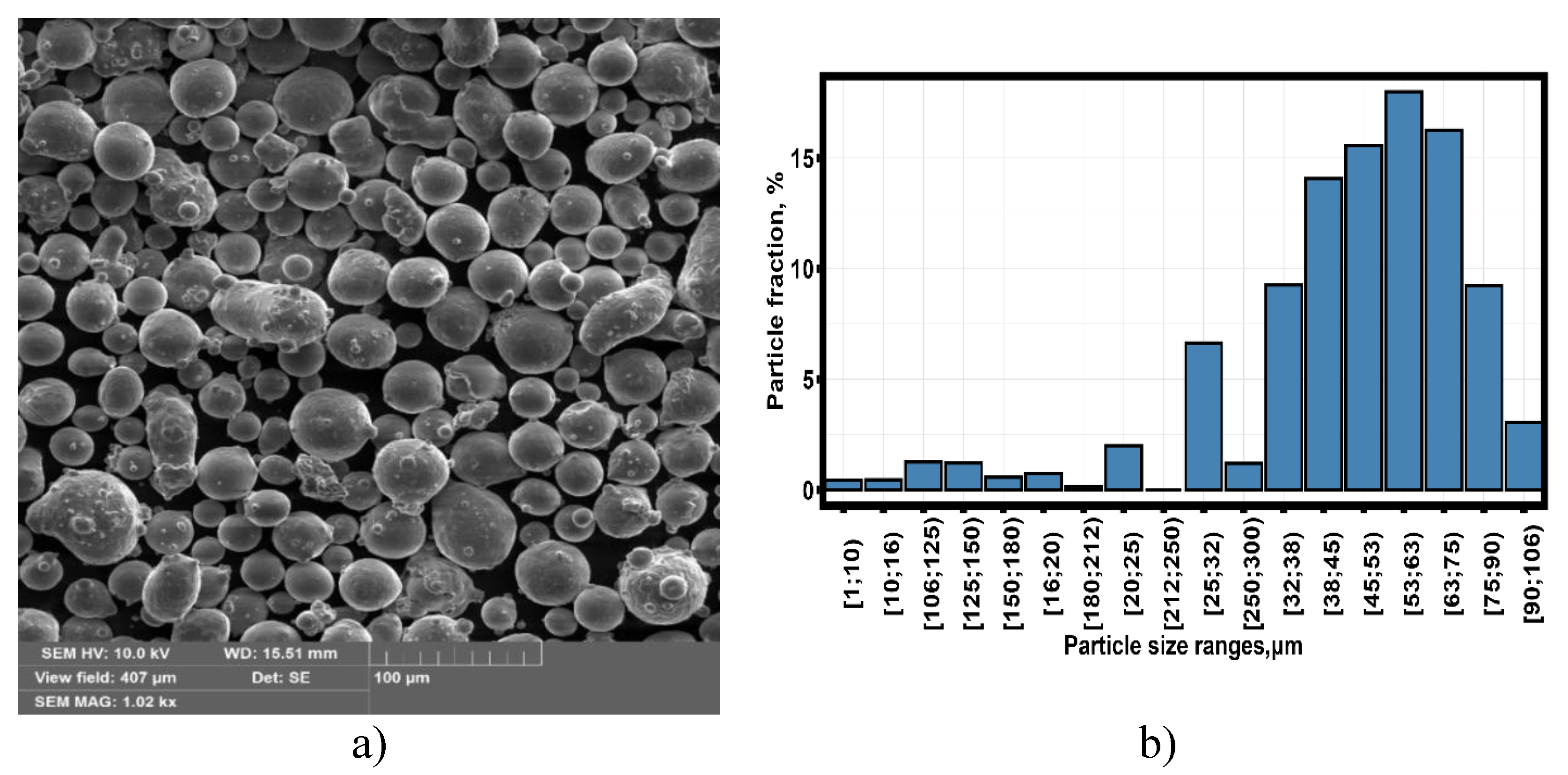
Figure 2.
– Thin-walled sample obtained by SLM: a) dimensions, and b) their location on the substrate plate.
Figure 2.
– Thin-walled sample obtained by SLM: a) dimensions, and b) their location on the substrate plate.
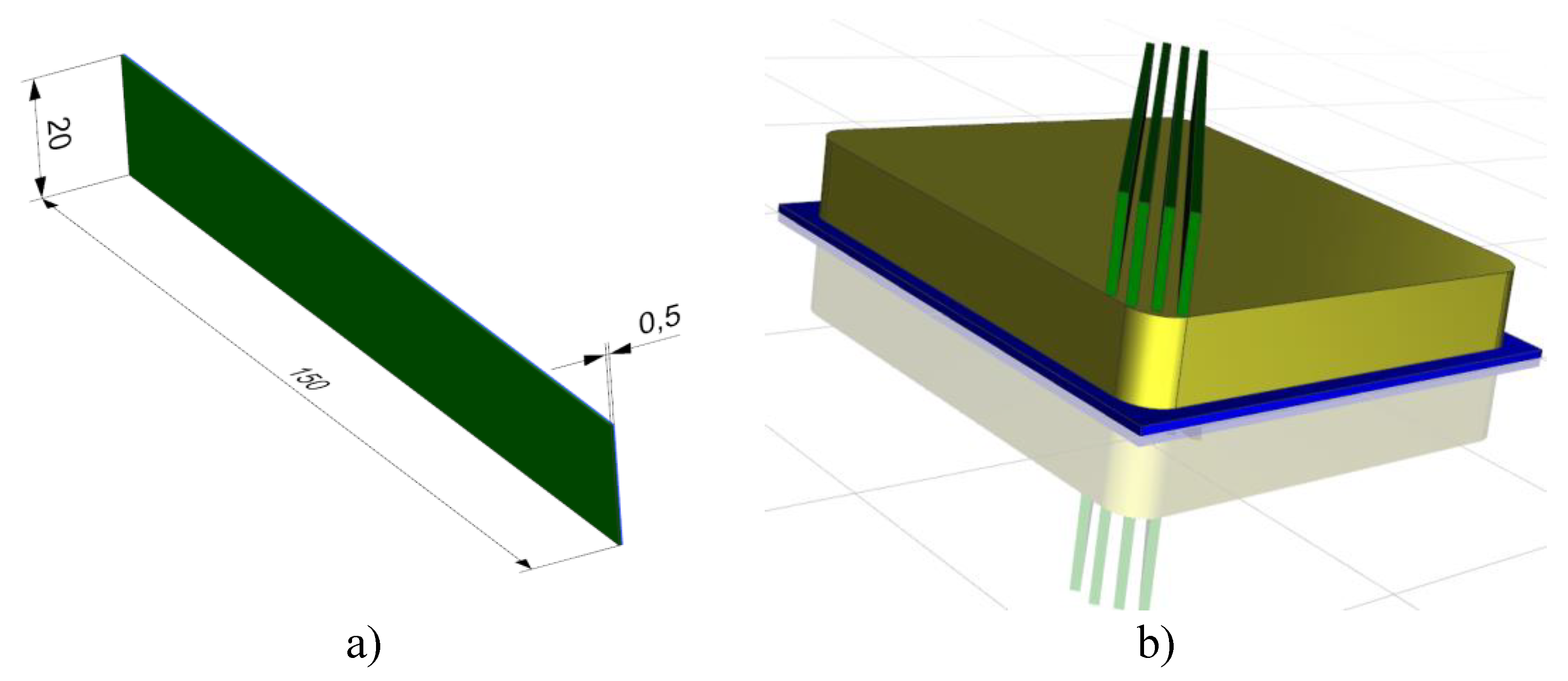
Figure 3.
- Tensile testing: a) samples after test, and b) INSTRON 5989 tensile machine.

Figure 4.
- Algorithm of statistical analysis of experimental results with verification of modeling results.
Figure 4.
- Algorithm of statistical analysis of experimental results with verification of modeling results.
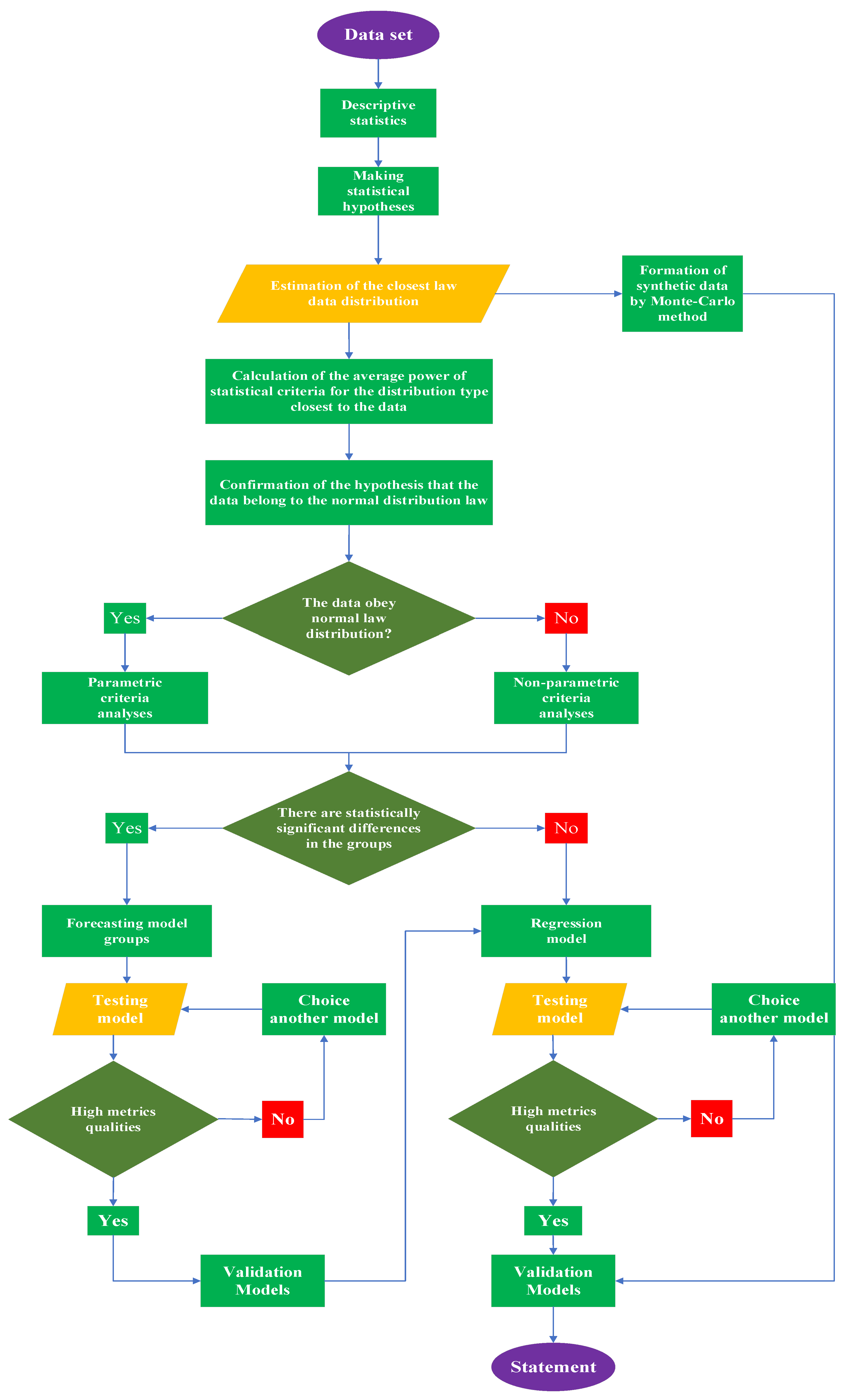
Figure 5.
- Algorithm for modeling validation data based on Monte Carlo method, regression equations and annealing method.
Figure 5.
- Algorithm for modeling validation data based on Monte Carlo method, regression equations and annealing method.
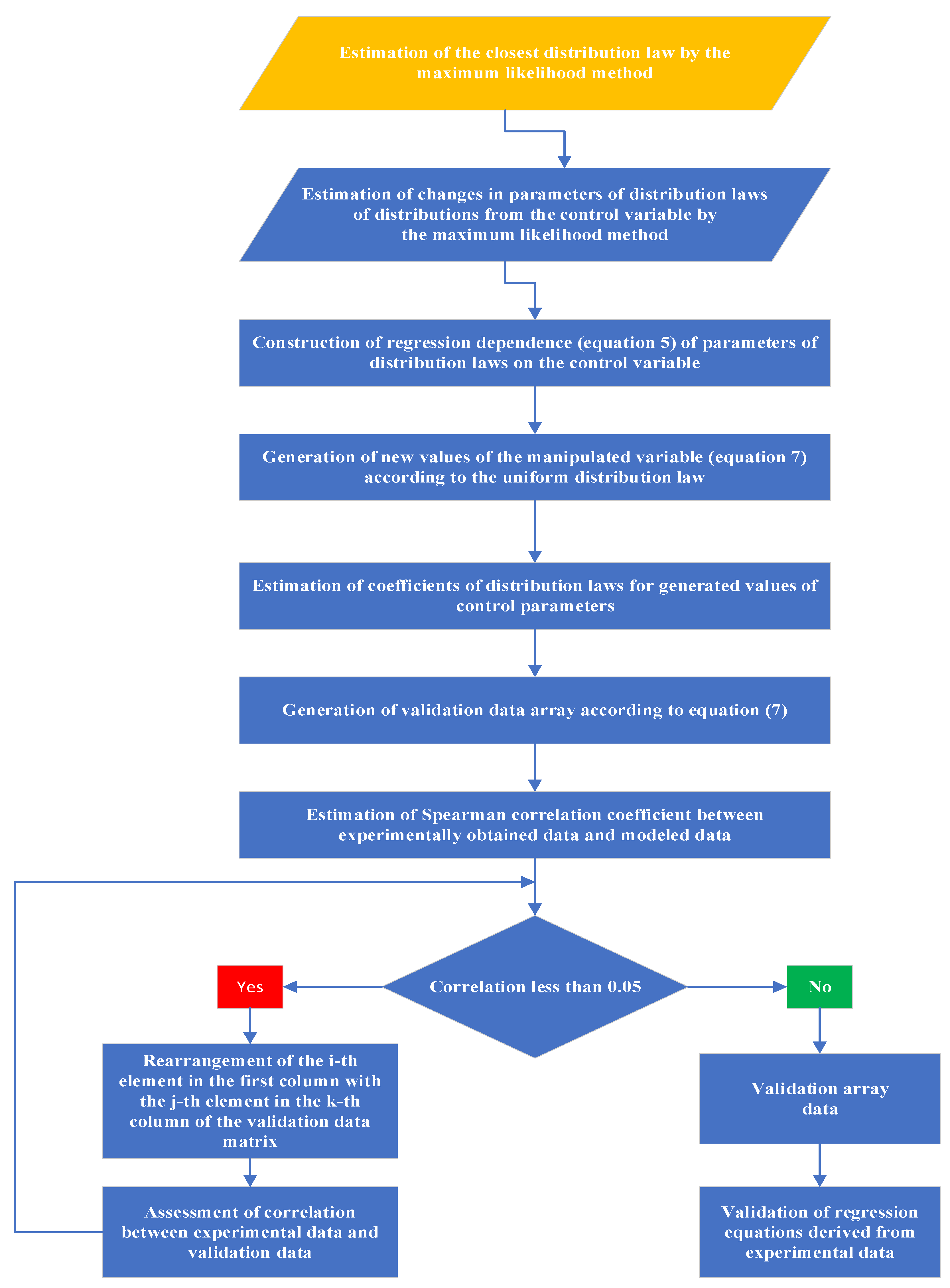
Figure 6.
– Stress-strain diagrams of SLMed Al-Mn-Mg-Ti-Zr thin-walled samples. a) Without heat treatment; b) Heat treatment at 260 ºC; c) Heat treatment at 290 ºC; d) Heat treatment at 320 ºC; e) Heat treatment at 350 ºC; f) Heat treatment at 380 ºC; g) Heat treatment at 410 ºC; h) Heat treatment at 440 ºC; i) Heat treatment at 470 ºC; j) Heat treatment at 500 ºC; k) Heat treatment at 530 ºC.
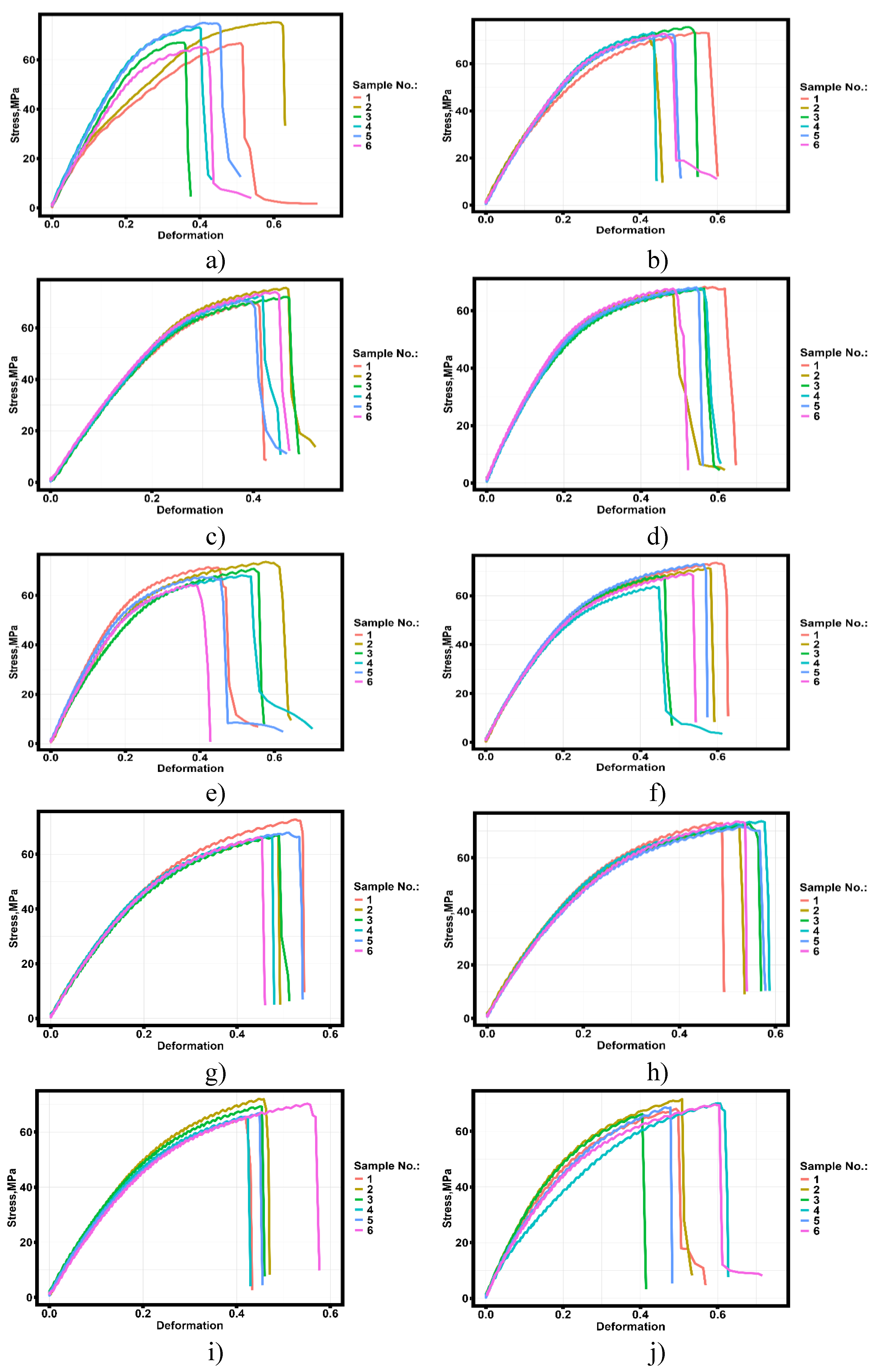
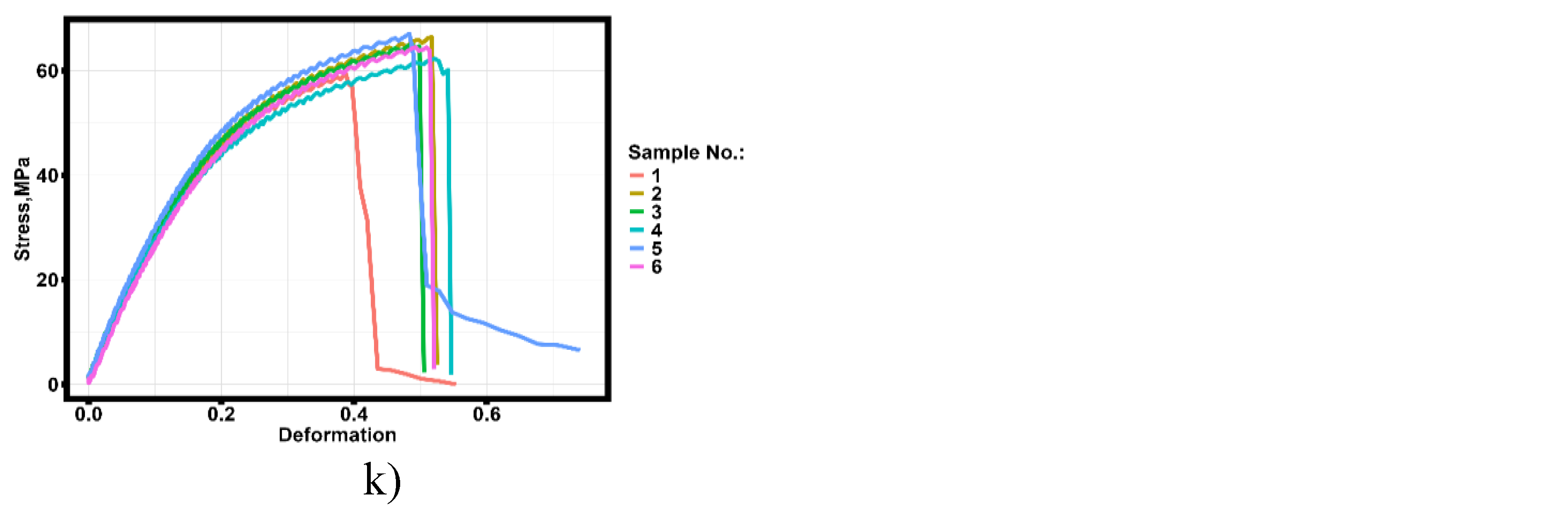
Figure 7.
- Surface roughness profiles of sandblasted Al-Mn-Mg-Ti-Zr alloy samples a) without heat treatment; b) before and c) after heat treatment at 260 ºС; d) before and e) after heat treatment at 290 ºC; f) before and g) after heat treatment at 320 ºC; h) before and i) after heat treatment at 350 ºC; j) before and k) after heat treatment at 380 ºC; l) before and m) after heat treatment at 410 ºC; n) before and o) after heat treatment at 440 ºC; p) before and q) after heat treatment at 470 ºC; r) before and s) after heat treatment at 500 ºC; t) before and u) after heat treatment at 530 ºC.
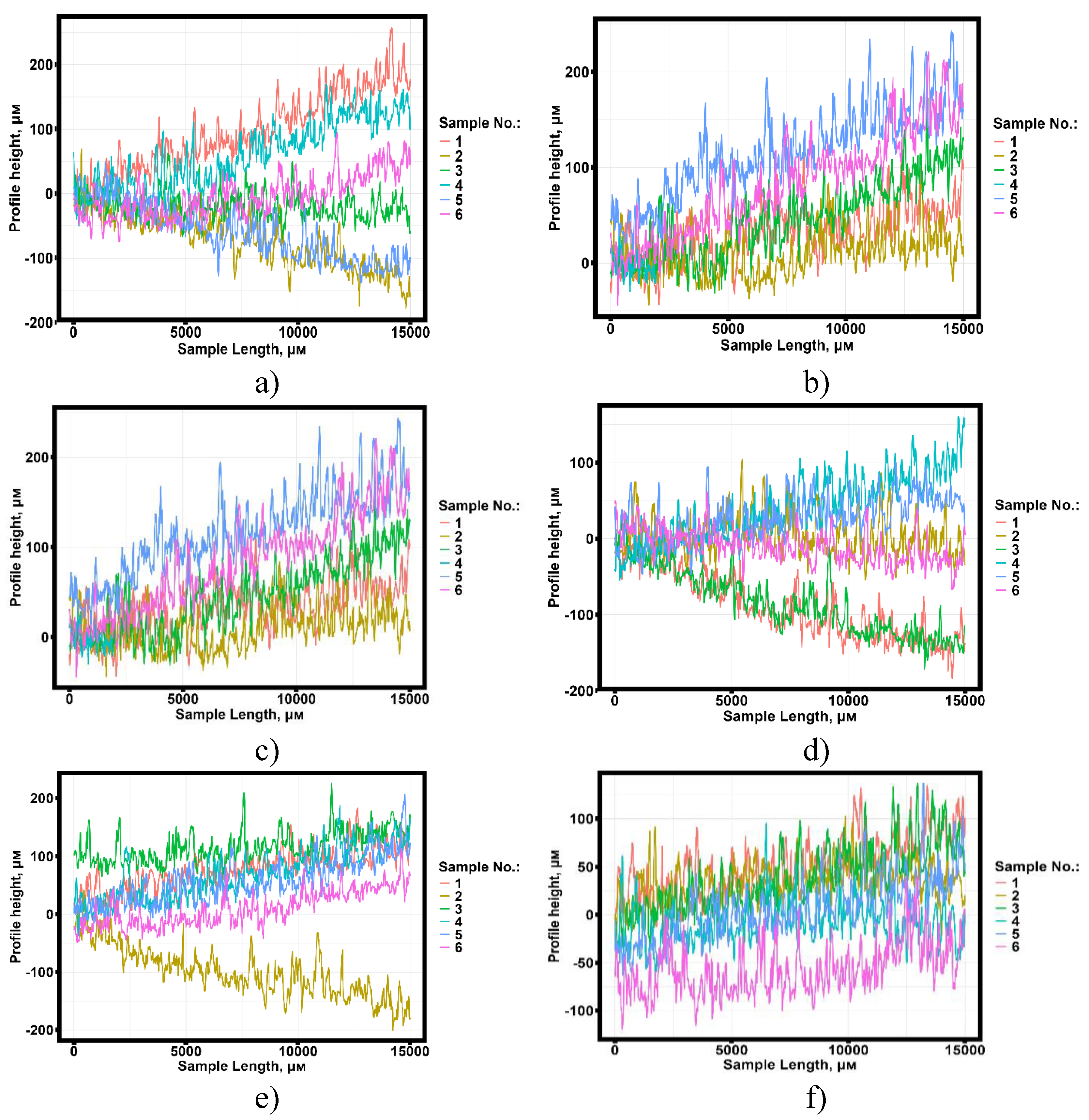
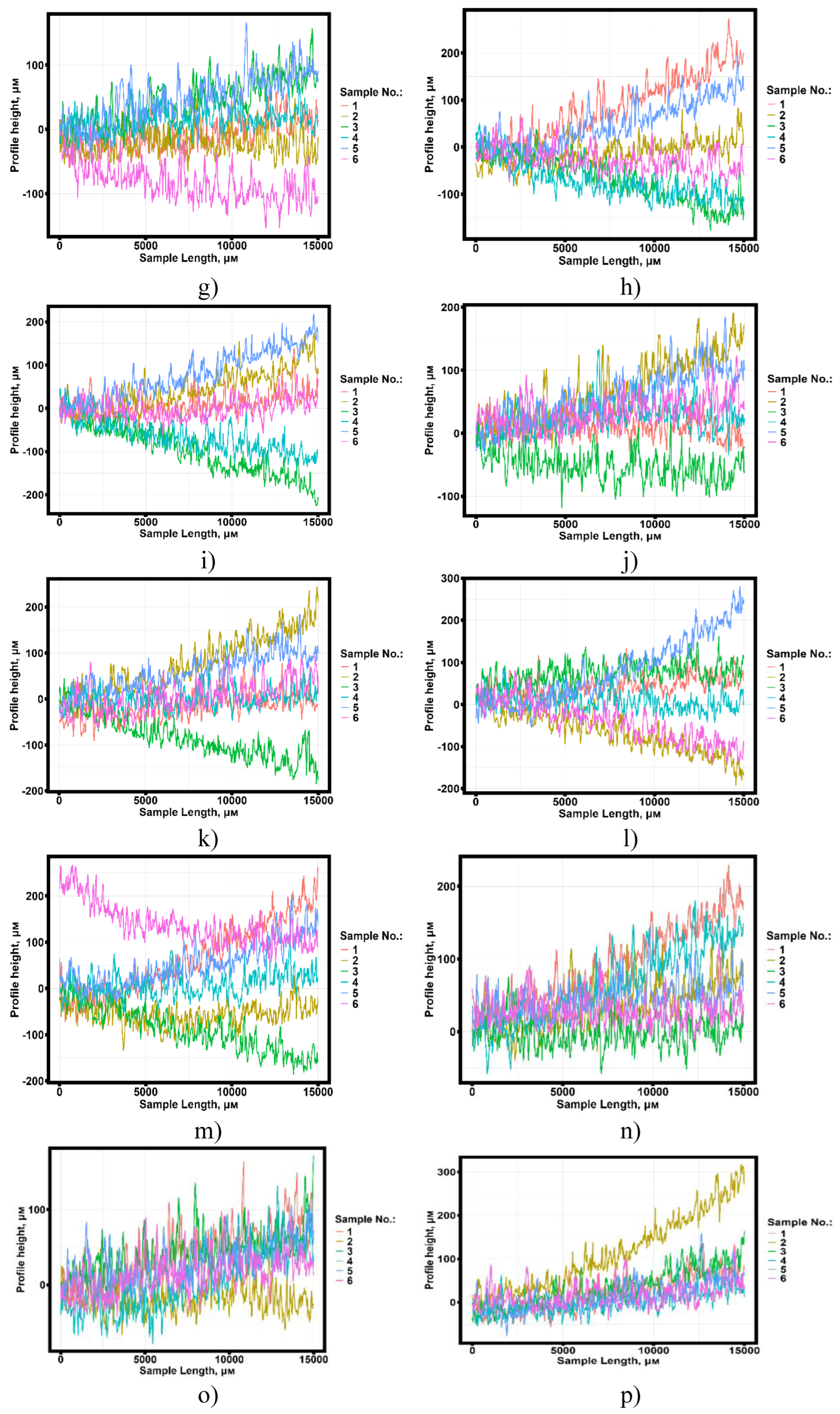
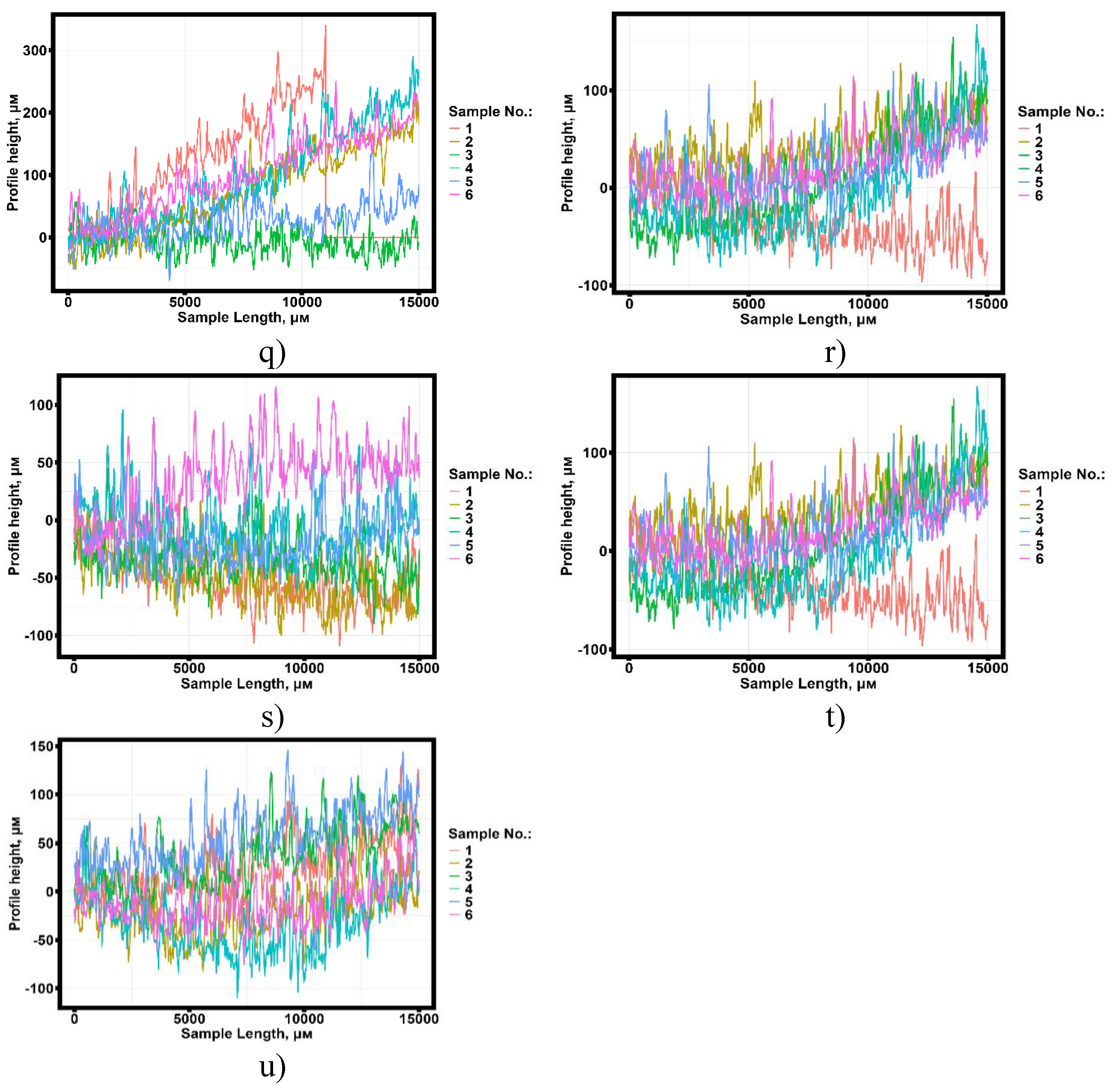
Figure 8.
- Dependence of the main investigated quantities on the heat treatment temperature. a) Young’s modulus; b) Secant modulus; c) Yield strength; d) Tensile strength; e) Strain corresponding to yield strength; f) Strain corresponding to tensile strength; g) Vickers microhardness; h) Ra; i) Rz; j).
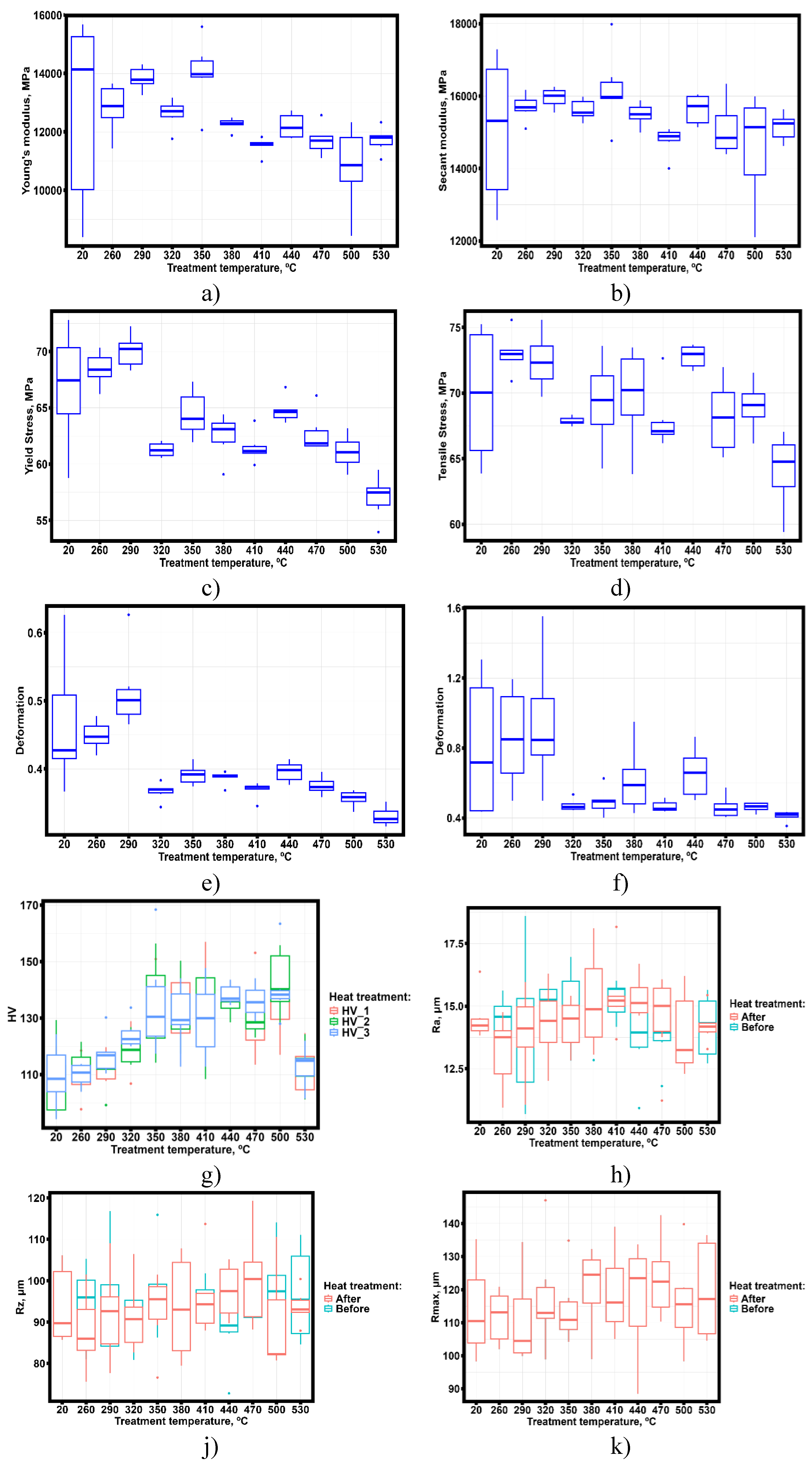
Figure 9.
- Dependence of strain hardening coefficient on heat treatment temperature SLMed Al-Mn-Mg-Ti-Zr thin-walled samples.
Figure 9.
- Dependence of strain hardening coefficient on heat treatment temperature SLMed Al-Mn-Mg-Ti-Zr thin-walled samples.
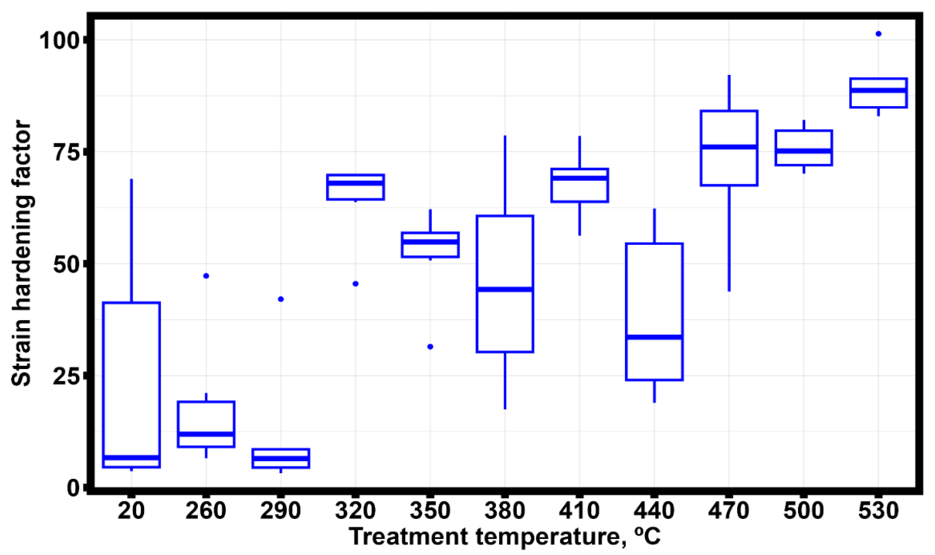
Figure 10.
- Dependence of the average statistical power of Shapiro-Wilk, D’Agusto, Kolmogorov-Smirnov, and Anderson-Darling criteria on the number of trials during testing the compliance the normal distribution of yield strength values for the a) normal; b) lognormal; c) logistic; d) gamma; e) Weibull; f) Gumbell; and g) Cauchy distributions.
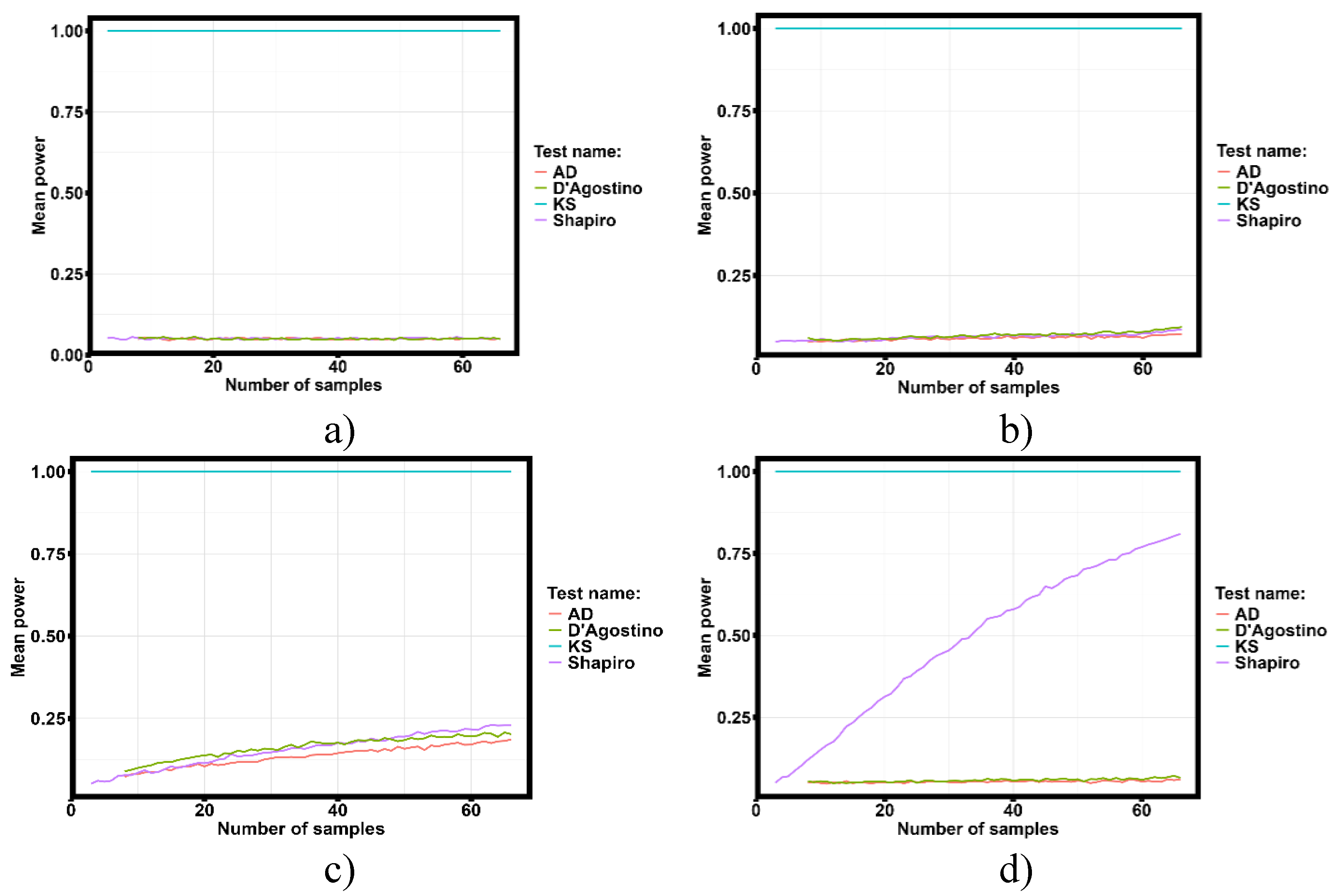
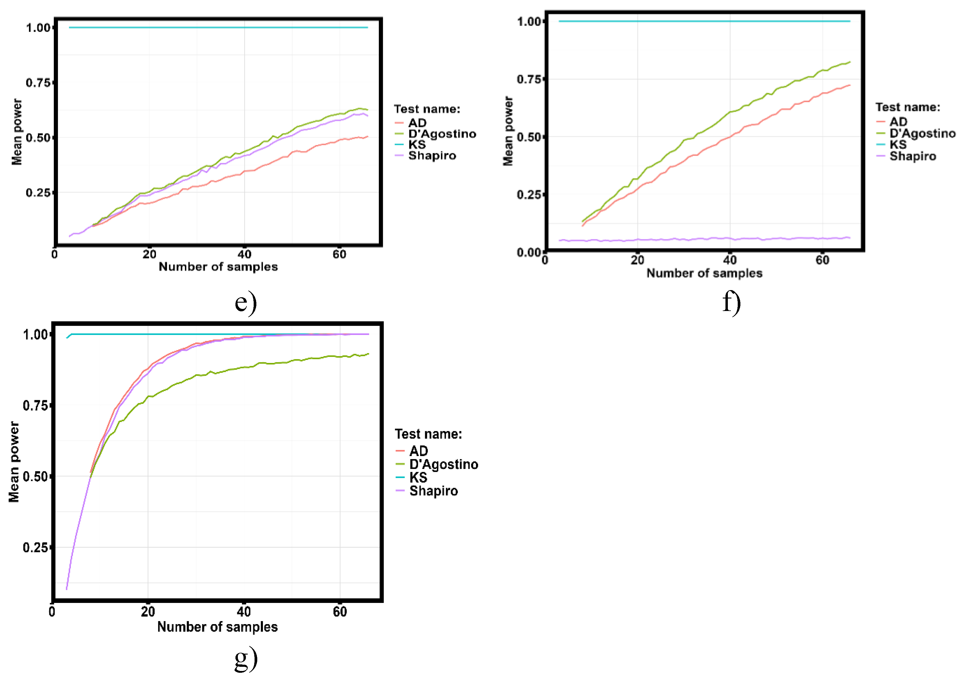
Figure 11.
- Spearman correlation analysis in three groups of tensile test results, surface roughness measurements and microhardness of thin-walled specimens produced by selective laser melting technology from Al-Mn-Mg alloy. a) Spearman correlation in group 1; b) Spearman correlation in group 2; c) Spearman correlation in group 3. Where T - heat treatment temperature; H - actual specimen thickness; W - actual specimen width; EY - Young’s modulus; ET - secant modulus; YS - yield strength; TS - tensile strength; RABHT - Ra before heat treatment; RZBHT - Rz before heat treatment; RMBHT - Rmax before heat treatment; RAAHT - Ra after heat treatment; RZAHT - Rz after heat treatment; RMAHT - Rmax after heat treatment; HV_1, HV_2 and HV_3 - Vickers microhardness in the first, second and third series of measurements; DTS - strain corresponding to the strength limit; DYS - strain corresponding to the yield limit; SHF - strain hardening factor.
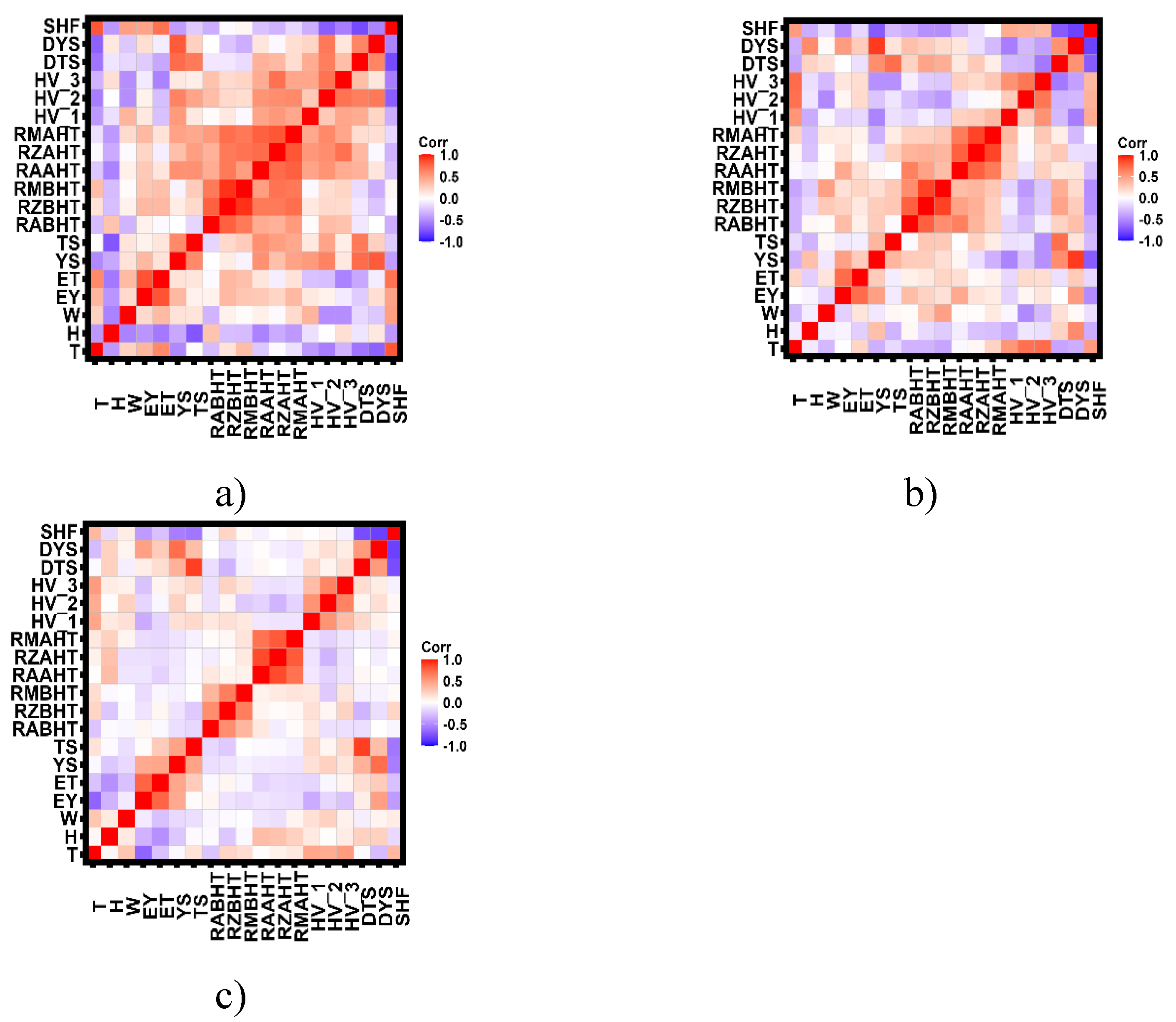
Figure 12.
- Correlation graphs between variables included in the dataset. a) Group 1; b) Group 2; c) Group 3. Where T - heat treatment temperature; H - actual specimen thickness; W - actual specimen width; EY - Young’s modulus; ET - secant modulus; YS - yield strength; TS - tensile strength; RABHT - Ra before heat treatment; RZBHT - Rz before heat treatment; RMBHT - Rmax before heat treatment; RAAHT - Ra after heat treatment; RZAHT - Rz after heat treatment; RMAHT - Rmax after heat treatment; HV_1, HV_2 and HV_3 - Vickers microhardness in the first, second and third series of measurements; DTS - strain corresponding to the strength limit; DYS - strain corresponding to the yield limit; SHF - strain hardening factor.
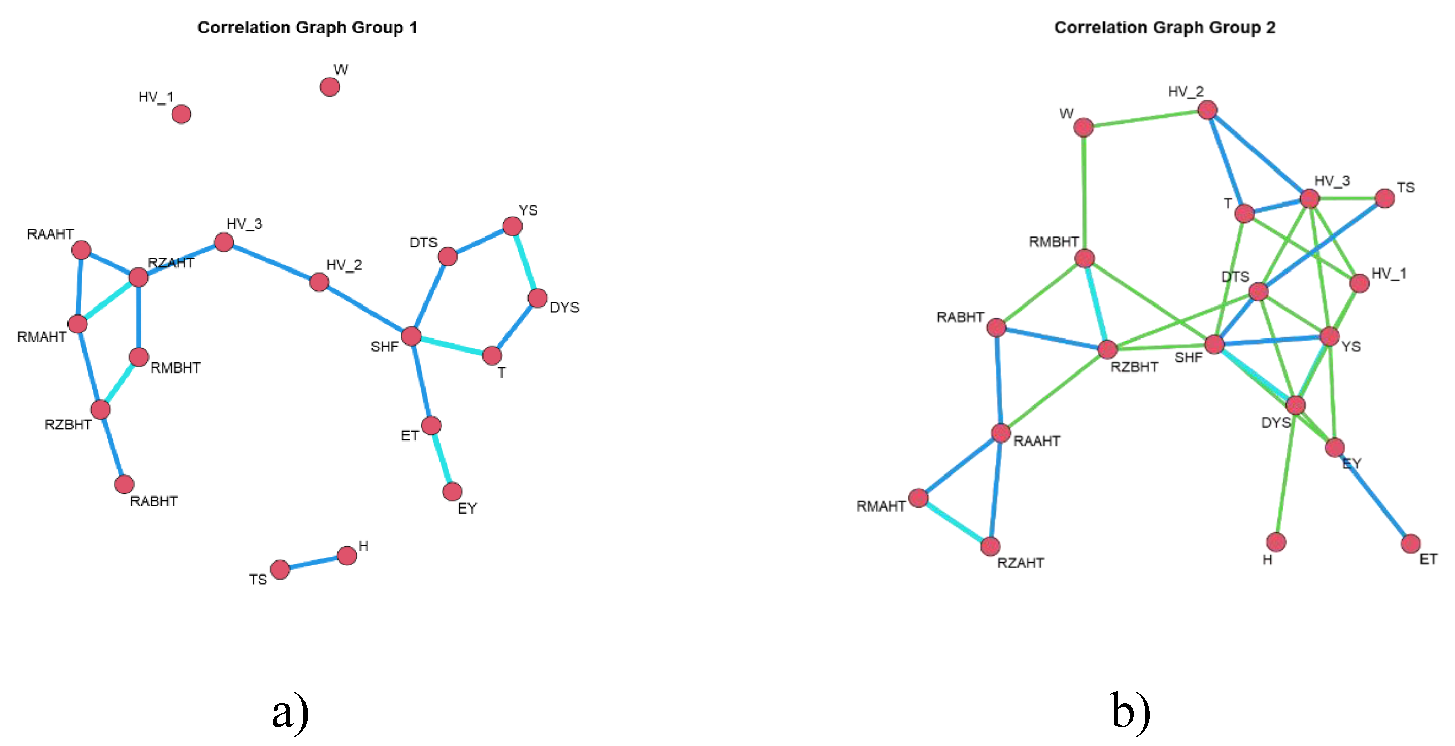
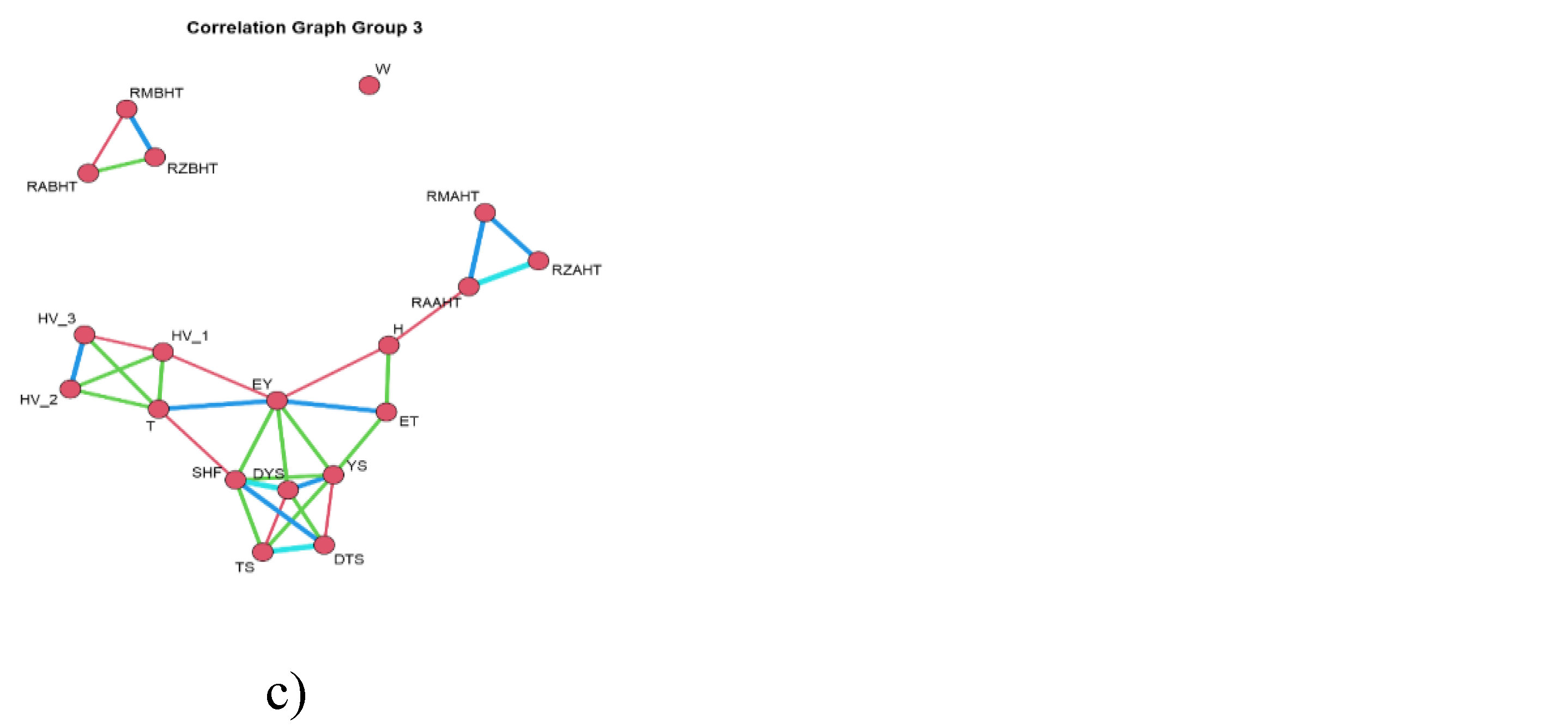
Figure 15.
- Histogram of the distribution of the annealing temperature generated by a uniform distribution law with a minimum temperature value of 20 ºC and a maximum temperature of 530 ºC.
Figure 15.
- Histogram of the distribution of the annealing temperature generated by a uniform distribution law with a minimum temperature value of 20 ºC and a maximum temperature of 530 ºC.

Figure 16.
- Dependence of predictions of the most significant values by robust regression equations (11)-(15) on the values obtained by Monte Carlo method. a) Scatter diagram of predicted values of Young’s modulus; b) Histogram of distribution of residuals of the difference of two models; c) Scatter diagram of predicted values of modulus along the secant; d) Histogram of distribution of residuals of model differences; e) Scatter diagram of predicted values of ultimate strength; f) Histogram of distribution of residuals; g) Scatter diagram of predicted values of strain hardening coefficient; h) Histogram of distribution of residuals of models; i) Scatter diagram of predicted values of strain corresponds to the strain rate of deformation; j) Histogram of distribution of residuals of models;.
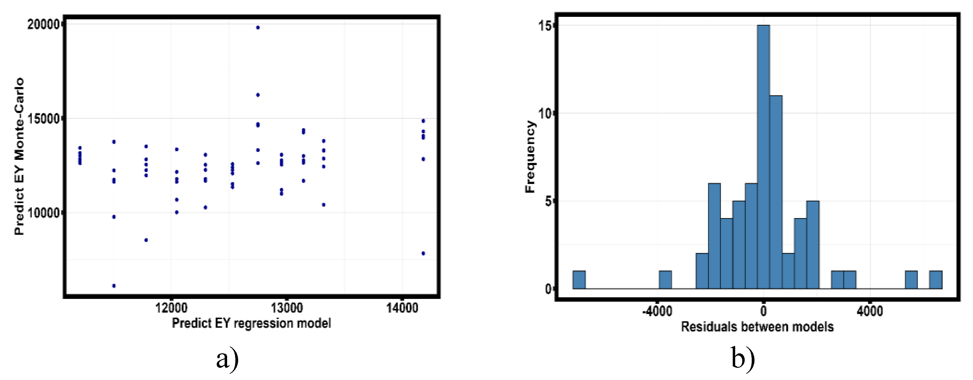
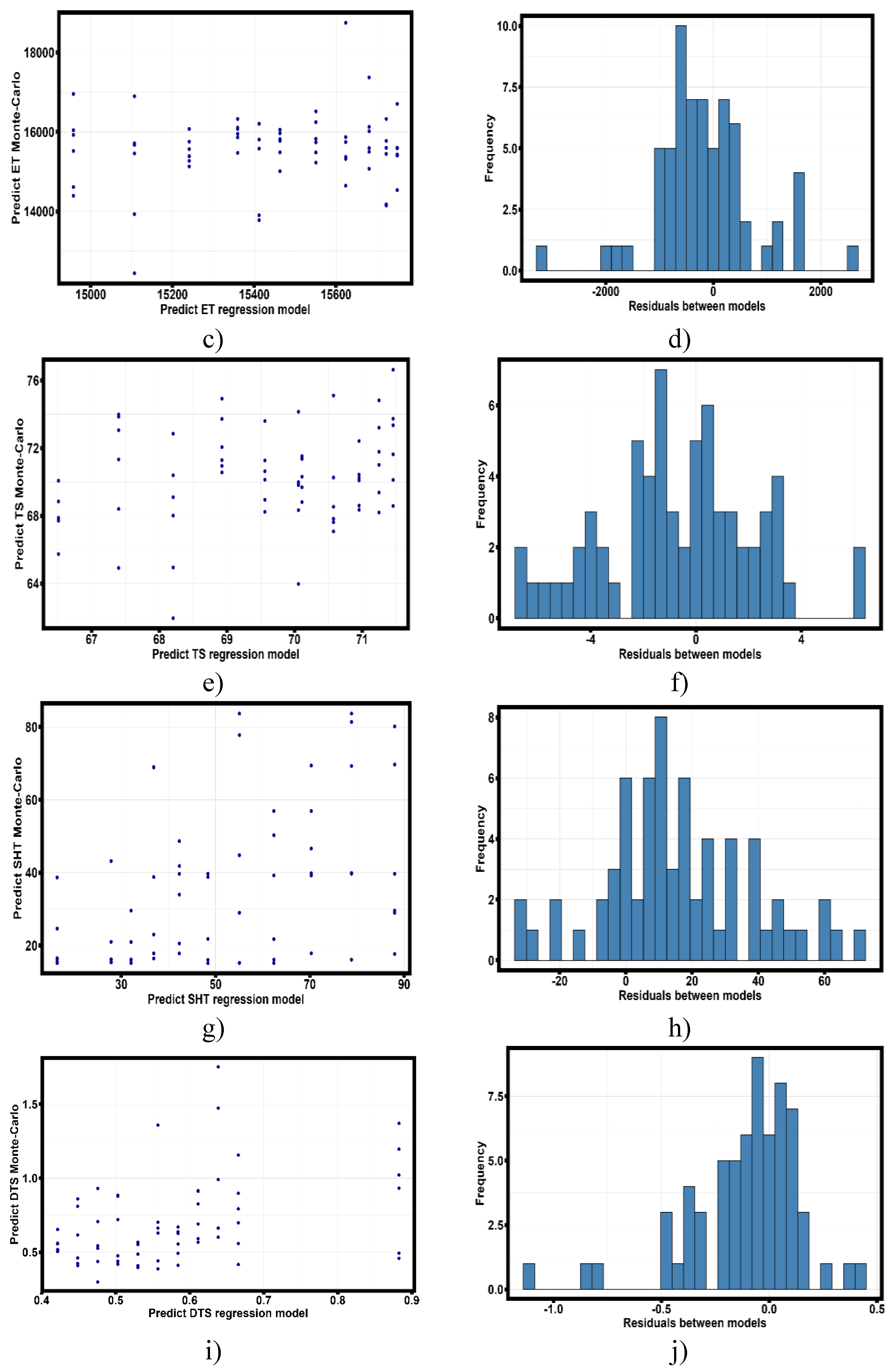
Figure 18.
- Results of X-ray phase analysis of heat treated at 290 ºC for 1 hour sample number 1 (HT 290), and samples number 1(WHT 1) and 5 (WHT 5) without heat treatment.
Figure 18.
- Results of X-ray phase analysis of heat treated at 290 ºC for 1 hour sample number 1 (HT 290), and samples number 1(WHT 1) and 5 (WHT 5) without heat treatment.
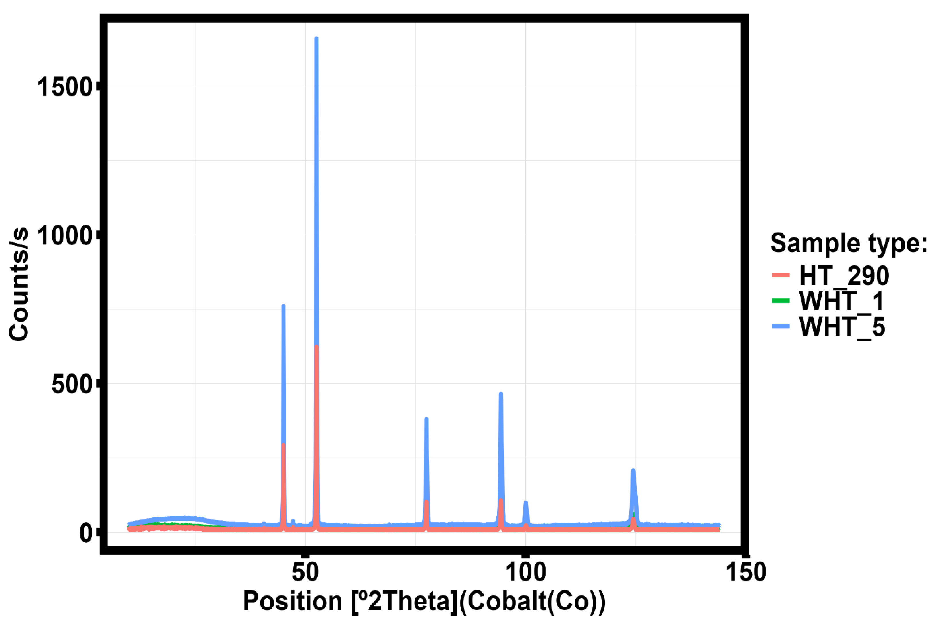
Figure 20.
- X-ray diffraction of thin-walled samples heat-treated at 410 ºC (HT 410) and 470 ºC (HT 470) for one hour.
Figure 20.
- X-ray diffraction of thin-walled samples heat-treated at 410 ºC (HT 410) and 470 ºC (HT 470) for one hour.
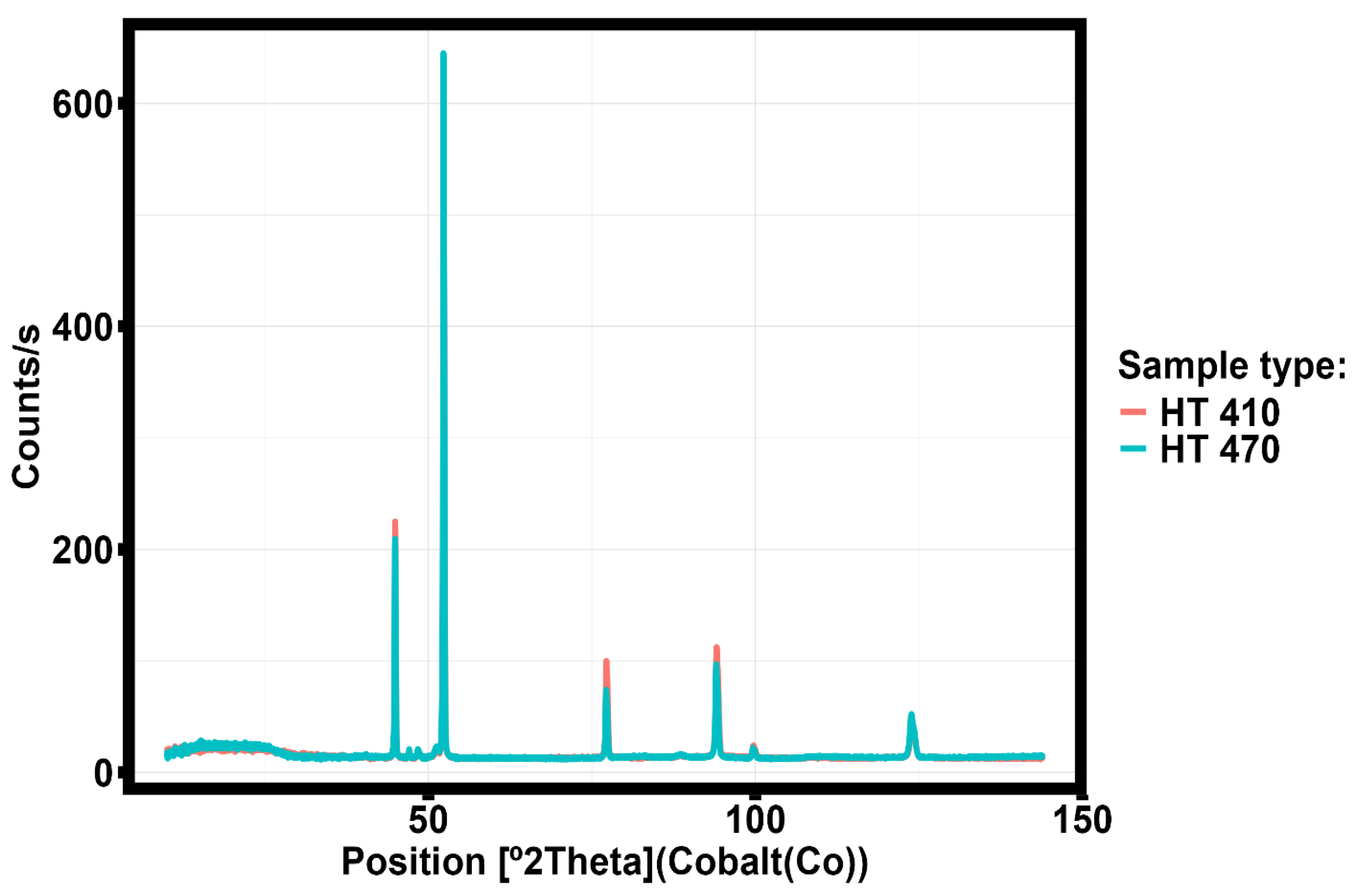
Figure 21.
- X-ray diffraction of thin-walled samples number 1 (HT 530_1) and 3 (HT 530_3) heat-treated at 530 ºC for one hour.
Figure 21.
- X-ray diffraction of thin-walled samples number 1 (HT 530_1) and 3 (HT 530_3) heat-treated at 530 ºC for one hour.
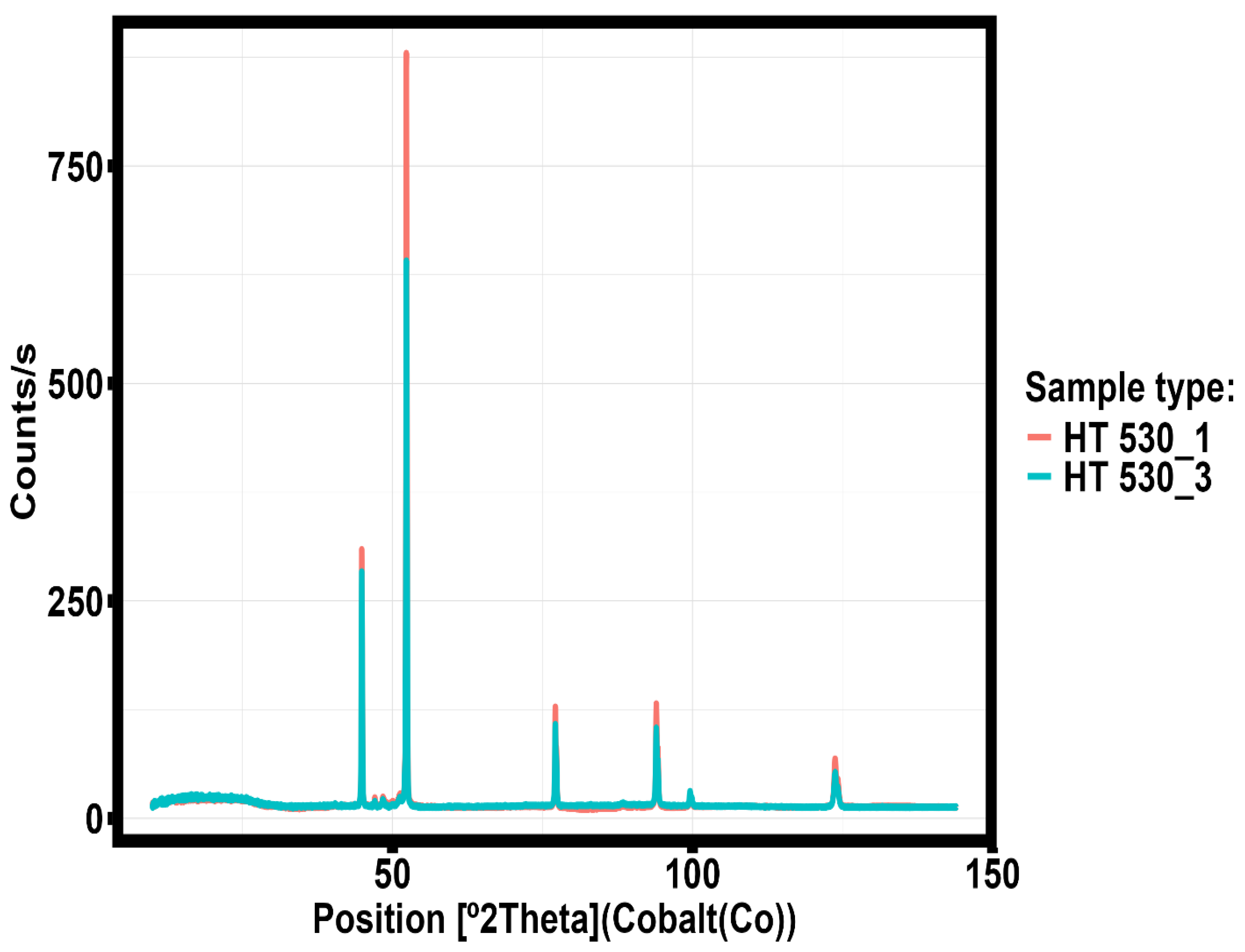

Table 1.
Chemical composition of the raw powder for the thin-walled samples.
| Measurement series | Element content, % wt. | ||||
|---|---|---|---|---|---|
| Al | Mn | Mg | Zr | Ti | |
| 1 | 94.34 | 3.04 | 2.39 | 0.14 | 0.09 |
| 2 | 93.97 | 3.53 | 2.27 | 0.11 | 0.12 |
| 3 | 93.61 | 3.78 | 2.41 | 0.09 | 0.11 |
Table 2.
Scheme of sample generation by equation (6).
| Var | Simulations | |||||
|---|---|---|---|---|---|---|
| 1 | 2 | 3 | … | … | Nsim | |
| X1 | x1,1 | x1,2 | x1,3 | … | … | x1,Nsim |
| X2 | x2,1 | x2,2 | x2,3 | … | … | x2,Nsim |
| … | … | … | … | … | … | … |
| XNvar | x1,Nvar | xNvar,2 | xNvar,3 | … | … | x1,Nsim |
Table 3.
Results of the analysis of the closest law of distribution by Akaike and Bayesian information criteria.
Table 3.
Results of the analysis of the closest law of distribution by Akaike and Bayesian information criteria.
| Variable | Criterion | Distribution law | |||||||
|---|---|---|---|---|---|---|---|---|---|
| Normal | LogNorm | Logistic | Gamma | Weibull | Exp. | Gumbell | Cauchy | ||
| EY, MPa | Akaike | 543.022 | 546.942 | 539.581 | 545.189 | 546.899 | 770.173 | 561.671 | 550.118 |
| Bayes | 547.401 | 551.322 | 543.960 | 549.568 | 551.278 | 772.362 | 566.050 | 554.497 | |
| ET, MPa | Akaike | 487.725 | 492.355 | 478.043 | 490.666 | 487.627 | 798.782 | 519.767 | 482.978 |
| Bayes | 492.104 | 496.734 | 482.423 | 495.045 | 492.007 | 800.971 | 524.146 | 487.357 | |
| σ0.2, MPa | Akaike | 376.311 | 375.531 | 378.407 | 375.713 | 385.520 | 682.351 | 380.241 | 398.717 |
| Bayes | 380.690 | 379.911 | 382.786 | 380.093 | 389.900 | 684.540 | 384.620 | 403.097 | |
| σB, MPa | Akaike | 357.990 | 359.246 | 361.612 | 358.778 | 356.914 | 693.824 | 373.096 | 392.362 |
| Bayes | 362.369 | 363.625 | 365.999 | 363.157 | 361.294 | 696.014 | 377.475 | 396.741 | |
| ε0.2 | Akaike | -176.865 | -191.149 | -188.262 | -186.863 | -157.173 | 13.121 | -205.074 | -196.006 |
| Bayes | -172.486 | -186.770 | -183.882 | -182.484 | -152.793 | 15.311 | -200.695 | -191.627 | |
| εB | Akaike | 11.803 | -24.168 | 2.234 | -14.018 | 4.100 | 67.544 | -26.774 | -31.021 |
| Bayes | 16.182 | -19.789 | 6.613 | -9.639 | 8.479 | 69.734 | -22.394 | -26.642 | |
| HV_1 | Akaike | 539.507 | 538.563 | 542.762 | 538.660 | 545.670 | 770.359 | 541.664 | 568.507 |
| Bayes | 543.887 | 542.942 | 547.142 | 543.040 | 550.049 | 772.548 | 546.043 | 572.887 | |
| HV_2 | Akaike | 546.838 | 546.405 | 550.042 | 546.297 | 552.062 | 771.179 | 550.850 | 577.117 |
| Bayes | 551.218 | 550.784 | 554.421 | 550.676 | 556.441 | 773.369 | 555.230 | 581.497 | |
| HV_3 | Akaike | 543.861 | 542.396 | 545.455 | 542.613 | 553.211 | 772.274 | 545.954 | 572.888 |
| Bayes | 548.241 | 546.776 | 549.835 | 546.992 | 557.590 | 774.464 | 550.333 | 577.267 | |
| Ra, μm, Before heat treatment | Akaike | 239.457 | 242.814 | 239.040 | 241.443 | 241.777 | 486.966 | 256.755 | 261.134 |
| Bayes | 243.836 | 247.194 | 243.420 | 245.822 | 246.157 | 489.156 | 261.135 | 265.513 | |
| Ra, μm, After heat treatment | Akaike | 241.394 | 243.092 | 240.343 | 242.265 | 246.914 | 486.481 | 254.274 | 258.246 |
| Bayes | 245.773 | 247.471 | 244.722 | 246.644 | 251.293 | 488.671 | 258.654 | 262.625 | |
| Rz, μm, Before heat treatment | Akaike | 479.917 | 479.245 | 481.351 | 479.281 | 488.437 | 734.804 | 485.079 | 506.335 |
| Bayes | 484.296 | 483.624 | 485.730 | 483.661 | 492.817 | 736.994 | 489.458 | 510.714 | |
| Rz, μm, After heat treatment | Akaike | 489.237 | 487.736 | 491.981 | 488.052 | 497.673 | 733.049 | 489.731 | 517.015 |
| Bayes | 493.617 | 492.115 | 496.360 | 492.431 | 502.053 | 735.239 | 494.111 | 521.395 | |
| Rmax, μm, Before heat treatment | Akaike | 529.931 | 528.558 | 533.977 | 528.815 | 536.285 | 762.389 | 530.644 | 561.836 |
| Bayes | 534.311 | 532.937 | 538.356 | 533.194 | 540.664 | 764.578 | 535.024 | 566.215 | |
| Rmax, μm, After heat treatment | Akaike | 555.467 | 550.152 | 555.052 | 551.536 | 568.393 | 759.734 | 548.390 | 577.165 |
| Bayes | 559.846 | 554.531 | 559.431 | 555.915 | 572.772 | 761.924 | 552.770 | 581.544 | |
Table 4.
Results of testing the conformity of the law of distribution of experimental data to the normal law of distribution by the Kolmogorov-Smirnov criterion.
Table 4.
Results of testing the conformity of the law of distribution of experimental data to the normal law of distribution by the Kolmogorov-Smirnov criterion.
| Investigated value | Kolmogorov-Smirnov statistics | |
|---|---|---|
| p-value | D | |
| EY, MPa | <0.0000001 | 1.000 |
| ET, MPa | <0.0000001 | 1.000 |
| σ0.2, MPa | <0.0000001 | 1.000 |
| σB, MPa | <0.0000001 | 1.000 |
| ε0.2 | <0.0000001 | 0.624 |
| εB | <0.0000001 | 0.641 |
| HV_1 | <0.0000001 | 1.000 |
| HV_2 | <0.0000001 | 1.000 |
| HV_3 | <0.0000001 | 1.000 |
| Ra, μm, Before heat treatment | <0.0000001 | 1.000 |
| Ra, μm, After heat treatment | <0.0000001 | 1.000 |
| Rz, μm, Before heat treatment | <0.0000001 | 1.000 |
| Rz, μm, After heat treatment | <0.0000001 | 1.000 |
| Rmax, μm, Before heat treatment | <0.0000001 | 1.000 |
| Rmax, μm, After heat treatment | <0.0000001 | 1.000 |
Table 5.
Results of Kruskal-Wallis test with Dunn’s criterion and Bonferroni multiple comparison correction (only groups with statistically significant differences are presented).
Table 5.
Results of Kruskal-Wallis test with Dunn’s criterion and Bonferroni multiple comparison correction (only groups with statistically significant differences are presented).
| Parameter | Comparable groups | p-value |
|---|---|---|
| EY, MPa | 290 - 410 | 0.0106 |
| 350 - 410 | 0.0150 | |
| 290 - 500 | 0.0078 | |
| 350 - 500 | 0.0112 | |
| ET, MPa | 290 - 410 | 0.0489 |
| σ0.2, MPa | 290 - 320 | 1.2613e-02 |
| 290 - 410 | 1.8967e-02 | |
| 290 - 500 | 9.9428e-03 | |
| 20 - 530 | 6.9146e-03 | |
| 260 - 530 | 1.8546e-04 | |
| 290 - 530 | 1.8890e-05 | |
| 440 - 530 | 1.6898e-02 | |
| σB, MPa | 260 - 530 | 0.0028 |
| 290 - 530 | 0.0096 | |
| 440 - 530 | 0.0025 | |
| ε0.2 | 290 - 320 | 1.2190e-02 |
| 290 - 410 | 3.4161e-02 | |
| 20 - 500 | 3.6101e-02 | |
| 260 - 500 | 4.4592e-03 | |
| 290 - 500 | 4.8312e-04 | |
| 20 - 530 | 2.2078e-03 | |
| 260 - 530 | 1.9099e-04 | |
| 290 - 530 | 1.4744e-05 | |
| εB | 260 - 530 | 0.0014 |
| 290 - 530 | 0.0008 | |
| 440 - 530 | 0.0126 | |
| HV_1 | 260 - 410 | 0.0371 |
| 20 - 440 | 0.0112 | |
| 260 - 440 | 0.0042 | |
| 290 - 440 | 0.0414 | |
| 260 - 500 | 0.0462 | |
| 440 - 530 | 0.0306 | |
| HV_2 | 20 - 500 | 0.0096 |
| 260 - 500 | 0.0238 | |
| 290 - 500 | 0.0298 | |
| 500 - 530 | 0.0212 | |
| HV_3 | 20 - 440 | 0.0225 |
| 260 - 440 | 0.0085 | |
| 260 - 470 | 0.0212 | |
| 20 - 500 | 0.0206 | |
| 260 - 500 | 0.0078 | |
| 500 - 530 | 0.0463 |
Table 6.
The result of applying the hierarchical clustering method to the results of tensile tests, microhardness measurements and surface roughness parameters of samples obtained by selective laser melting from Al-Mn-Mg-Ti-Zr alloy and subjected to heat treatment.
Table 6.
The result of applying the hierarchical clustering method to the results of tensile tests, microhardness measurements and surface roughness parameters of samples obtained by selective laser melting from Al-Mn-Mg-Ti-Zr alloy and subjected to heat treatment.
| Group 1 | Group 2 | Group 3 | |||
|---|---|---|---|---|---|
| Sample number | Temperature, ºC | Sample number | Temperature, ºC | Sample number | Temperature, ºC |
| 1 | 20 | 2 | 20 | 6 | 20 |
| 4 | 380 | 3 | 20 | 1 | 320 |
| 4 | 500 | 4 | 20 | 2 | 320 |
| 1 | 530 | 5 | 20 | 3 | 320 |
| 2 | 530 | 1 | 260 | 4 | 320 |
| 3 | 530 | 2 | 260 | 5 | 320 |
| 4 | 530 | 3 | 260 | 6 | 320 |
| 5 | 530 | 4 | 260 | 3 | 350 |
| 6 | 530 | 5 | 260 | 4 | 350 |
| --- | --- | 6 | 260 | 5 | 350 |
| --- | --- | 1 | 290 | 6 | 350 |
| --- | --- | 2 | 290 | 1 | 380 |
| --- | --- | 3 | 290 | 2 | 380 |
| --- | --- | 4 | 290 | 3 | 380 |
| --- | --- | 5 | 290 | 5 | 380 |
| --- | --- | 6 | 290 | 6 | 380 |
| --- | --- | 1 | 350 | 1 | 410 |
| --- | --- | 2 | 350 | 2 | 410 |
| --- | --- | 1 | 440 | 3 | 410 |
| --- | --- | 2 | 470 | 4 | 410 |
| --- | --- | --- | --- | 5 | 410 |
| --- | --- | --- | --- | 6 | 410 |
| --- | --- | --- | --- | 1 | 470 |
| --- | --- | --- | --- | 3 | 470 |
| --- | --- | --- | --- | 4 | 470 |
| --- | --- | --- | --- | 5 | 470 |
| --- | --- | --- | --- | 6 | 470 |
| --- | --- | --- | --- | 1 | 500 |
| --- | --- | --- | --- | 2 | 500 |
| --- | --- | --- | --- | 3 | 500 |
| --- | --- | --- | --- | 5 | 500 |
| --- | --- | --- | --- | 6 | 500 |
Table 7.
Robust regression equations of the parameters making the main contribution to the error of equations (8)-(10).
Table 7.
Robust regression equations of the parameters making the main contribution to the error of equations (8)-(10).
| Equation | MSE | Eq. No |
|---|---|---|
| 964.300 | (11) | |
| 600.000 | (12) | |
| 4.047 | (13) | |
| 20.660 | (14) | |
| 0.134 | (15) |
Table 8.
Confidence intervals of robust regression coefficients determined by bootstrapping method at 95% confidence level.
Table 8.
Confidence intervals of robust regression coefficients determined by bootstrapping method at 95% confidence level.
| Eq. No. | Coefficient | Lower value of the coefficient (confidence level, 2.5%) | Upper value of the coefficient (confidence level, 97.5%) |
|---|---|---|---|
| 11 | Free term | 12025.705 | 12773.212 |
| Coefficient at T | -9020.824 | 3097.027 | |
| Coefficient at T2 | -9057.687 | 925.873 | |
| 12 | Free term | 15162.521 | 15646.709 |
| Coefficient at T | -4162.416 | 3488.653 | |
| Coefficient at T2 | -5346.453 | 682.655 | |
| 13 | Free term | 68.718 | 70.361 |
| Coefficient at T | -17.770 | 1.395 | |
| Coefficient at T2 | -17.483 | -1.134 | |
| 14 | Free term | 45.003 | 56.926 |
| Coefficient at T | 85.282 | 194.341 | |
| Coefficient at T2 | 19.225 | 120.642 | |
| 15 | Free term | 0.493 | 0.643 |
| Coefficient at T | -1.641 | -0.103 |
Table 9.
Root mean square error (RMSE) analysis of the theoretical PDF from the empirical PDF.
| Variable | Distribution law | RMSE |
|---|---|---|
| EY, MPa | Cauchy | 0.048 |
| Gumbell | 0.080 | |
| Weibull | 0.066 | |
| Logistic | 0.041 | |
| Log Normal | 0.052 | |
| Normal | 0.050 | |
| Gamma | 0.070 | |
| ET, MPa | Cauchy | 0.049 |
| Gumbell | 0.116 | |
| Weibull | 0.066 | |
| Logistic | 0.037 | |
| Log Normal | 0.073 | |
| Normal | 0.065 | |
| Gamma | 0.050 | |
| σB, MPa | Cauchy | 0.059 |
| Gumbell | 0.050 | |
| Weibull | 0.047 | |
| Logistic | 0.047 | |
| Log Normal | 0.042 | |
| Normal | 0.043 | |
| Gamma | 0.043 | |
| εB | Cauchy | 0.127 |
| Gumbell | 0.111 | |
| Weibull | 0.128 | |
| Logistic | 0.112 | |
| Log Normal | 0.112 | |
| Normal | 0.137 | |
| Gamma | 0.121 | |
| SHT | Cauchy | 0.081 |
| Gumbell | 0.086 | |
| Weibull | 0.097 | |
| Logistic | 0.062 | |
| Log Normal | 0.122 | |
| Normal | 0.068 | |
| Gamma | 0.107 |
Table 10.
Robust regression equations describe changes in the coefficients of distribution laws of a random variable from the temperature of heat treatment.
Table 10.
Robust regression equations describe changes in the coefficients of distribution laws of a random variable from the temperature of heat treatment.
| Variable | Distribution law | Coefficients |
|---|---|---|
| EY, MPa | Logistic | |
| ET, MPa | Logistic | |
| σB, MPa | Log Normal | |
| εB | Gumbell | |
| SHT | Logistic | |
Table 12.
Pearson correlation estimates between experimental data, robust regression predictions, and Monte Carlo predictions.
Table 12.
Pearson correlation estimates between experimental data, robust regression predictions, and Monte Carlo predictions.
| Variable | Correlation coefficient of Monte Carlo model and robust regression | Correlation coefficient of Monte Carlo model and experimental data | Correlation coefficient of regression model and experimental data |
|---|---|---|---|
| EY, MPa | 0.228 | 0.655 | 0.428 |
| ET, MPa | 0.107 | 0.641 | 0.344 |
| σB, MPa | 0.250 | 0.587 | 0.445 |
| εB | 0.403 | 0.661 | 0.473 |
| SHT | 0.447 | 0.545 | 0.706 |
Disclaimer/Publisher’s Note: The statements, opinions and data contained in all publications are solely those of the individual author(s) and contributor(s) and not of MDPI and/or the editor(s). MDPI and/or the editor(s) disclaim responsibility for any injury to people or property resulting from any ideas, methods, instructions or products referred to in the content. |
© 2025 by the authors. Licensee MDPI, Basel, Switzerland. This article is an open access article distributed under the terms and conditions of the Creative Commons Attribution (CC BY) license (http://creativecommons.org/licenses/by/4.0/).
Copyright: This open access article is published under a Creative Commons CC BY 4.0 license, which permit the free download, distribution, and reuse, provided that the author and preprint are cited in any reuse.


