
Submitted:
22 April 2025
Posted:
23 April 2025
You are already at the latest version
Abstract
Global Navigation Satellite System (GNSS), Internet of Things (IoT) and cloud computing technologies enable high-precision positioning service with flexible data communication, making real-time/near real-time monitoring more economical and efficient. In this study, a Multi-sensor GNSS-IoT System was developed for measuring precise water surface elevation (WSE). The system, which includes ultrasonic and accelerometer sensors, was deployed on a floating platform in Googong Reservoir, Australia, over a four-month period in 2024. WSE data derived from the system were compared against independent reference measurements from the reservoir operator, achieving an accuracy of 7 mm for daily solutions and 28 mm for epoch-by-epoch solutions. The results demonstrate the system’s potential for remote, autonomous WSE monitoring and its suitability for validating satellite Earth Observation data, particularly from the Surface Water and Ocean Topography (SWOT) mission. Despite environmental challenges such as moderate gale conditions, the system maintained robust performance, with over 90% of solutions meeting quality assurance standards. This research highlights the advantages of combining GNSS with IoT technologies and multiple sensors for cost-effective, long-term WSE monitoring in remote and dynamic environments. Future work will focus on optimizing accuracy and expanding applications to diverse aquatic settings.
Keywords:
hydrology
; low-cost GNSS
; water surface elevation
; satellite validation
; SWOT
1. Introduction
In December 2022, the American and French space agencies, NASA and CNES, launched the Surface Water and Ocean Topography (SWOT) satellite mission. This innovative new imaging radar mission hosts a bi-static Ka-band Synthetic Aperture Radar interferometer that is being used for the first time to generate maps of ocean and in-land water topography with un-precedented spatial resolution [1,2,3].
Early analysis of SWOT data products for Australia by Maubant et al found that water surface elevation (WSE) for on-farm water storages as small as 0.17 km2 can be resolved [4]. This opens up new possibilities in remote monitoring of in-land water usage and storage by water managers. However, if these observations are to be used in compliance, trust in the remotely-derived SWOT measurements needs to be established by undertaking robust ongoing validation with in-situ measurements for a range of water body types and environments.
Mission requirements for the WSE measurements from SWOT are 10 cm accuracy or better (1σ) for open-water areas larger than 1 km2, and water surface slope (WSS) accuracy of 1.7cm/km or better (1σ) over a maximum 10 km of flow distance [5,6]. To assess the performance of SWOT against these requirements, in-situ validation measurements with centimetric accuracy are required.
A range of different in-situ instruments can be used to measure WSE, and therefore validate satellite-derived measurements. These include manual readings, pressure gauges and acoustic gauges that have been widely used but often come with limitations in precision, response time, spatial coverage, and cost [7]. The advent of Global Navigation Satellite System (GNSS) technology has opened new possibilities for near real-time, high-precision WSE and WSS monitoring.
There are two main different methods to measure WSE using GNSS technology: one is by utilizing GNSS radio signals reflected from the water surface, called GNSS Reflectometry technique (GNSS-R), and the other is by deploying GNSS instruments on floating buoys and platforms to directly measure water surface vertical positioning. GNSS-R can calculate WSE based on either signal-to-noise ratio (SNR) or phase delay observations [8,9,10]. GNSS-R has been successfully demonstrated to retrieve WSE data on various types of water bodies, including those of seas, lakes, rivers, and reservoirs [11,12,13]. While these studies have demonstrated that GNSS-R technology can achieve a mm to cm level precision under calm water conditions, it has limitations including the undefined datum of measurements and requirement of installation on a fixed location.
On the other hand, this need for precision and flexibility has driven the development of various GNSS buoy systems. Schöne et al. (2003) explored the use of GPS offshore buoys and tide gauge benchmark control by GPS [14]. Lin et al. (2017) presents the development and testing of a GNSS buoy specifically designed to monitor WSE in estuaries and coastal areas, providing an efficient and accurate method for capturing WSE changes. The authors caution against using Precise Point Positioning (PPP) for real-time monitoring of tides and ocean waves due to its long convergence times, which render it unsuitable for such applications [15]. Knight et al. (2020) developed a low-cost (~£300 GBP) GNSS buoy for measuring coastal sea levels, demonstrating the potential for precise WSE measurements to achieve a mean difference of RMSE 1.4 cm between the GNSS-buoy and reference tide gauge [16]. The data processing for Knight et al’s experiment is based on post-processing kinematic (PPK) method using the RTKLIB software [17]. Prior to the satellite SWOT mission, Pitcher et al. (2020) developed and deployed the GNSS-mounted floating Water Surface Profiler (WaSP) system, which efficiently and accurately measures WSE and WSS in various surface water environments using Precise Point Positioning (PPP). This system was instrumental in validating the experimental airborne prototype AirSWOT's performance. Their 63 lake surveys and additional river profiles demonstrated that the WaSP system provides sufficient accuracy for validating the decimeter-level precision of both SWOT and AirSWOT [18]. Tidey and Odolinski (2023) explored the use of low-cost multi-GNSS, single-frequency RTK averaging for marine applications, focusing on its ability to achieve accurate stationary positioning and vertical tide measurements [19]. The vertical component of their Otago Harbour trials achieved ≤ 0.016m standard deviation (STD) over a 7.3 km baseline and ≤ 0.022m STD over a 27.4 km baseline. Their research also demonstrated the benefits of leveraging observations from multiple GNSS constellations instead of just GPS. Ng et al. (2024) integrated Ginan, an open-source GNSS toolkit developed by Geoscience Australia, with the Dark-water Inland Observatory Network at Googong reservoir, demonstrating real-time and post-processed PPP workflows. While real-time PPP was impacted by process noise and BeiDou SSR reliability, post-processed PPP achieved accuracy of 4.8 cm overall and 2.2 cm for daily average solutions [20]. Li et al. (2024) analysed long-term (2007-2020) GNSS and tide gauge data over French Polynesia to monitor absolute vertical land motions and absolute sea-level (ASL) changes. This study provided critical insights into the regional variations in sea-level rise and land subsidence, contributing to a better understanding of the dynamics affecting coastal areas with long-term data [21]. The GNSS data processing method was PPP and conducted by using PANDA software [22].
Despite the previously demonstrated effectiveness of GNSS buoys for WSE estimation, there are several challenges with their practical operation and maintenance and building this in to a low-cost package that is commercially viable for large-scale deployment. These problems include accuracy and precision [16,19], signal interference [18], power and maintenance [16], data fusion and complexity [15,23]. These challenges underscore the need for ongoing research and development to enhance the reliability, accuracy, and usability of low-cost GNSS technologies for monitoring WSE. Recent advances in low-cost GNSS and Internet of Things (IoT) technologies have enabled the development of compact automatic long-term surface displacement monitoring [24,25,26]. Building on these innovations, we designed a multi-sensor floating platform that integrates GNSS, ultrasonic ranging, and accelerometer data to achieve high-precision WSE measurements.
In this study, we develop a Multi-sensor GNSS-IoT System (hereafter, the “System”) to provide low-latency WSE measurements with sufficient accuracy and temporal resolution to be useful for SWOT product validation and other hydrological applications. We evaluate the accuracy by comparing its measurements with reference data while analyzing key error sources, such as ultrasonic sensor performance, and assessing its robustness under different weather conditions. In this contribution, we first introduce the details of the integrated multi-sensor GNSS-IoT water-level measuring platform, including its components, mathematical model, and error budget. Then, we describe an experiment at the Googong reservoir, Australia that we designed to test the accuracy of proposed water level measurement platform. Following discussion of the system overall performance, we conclude the main findings and propose future work.
2. Methodology
An end-to-end, automated GNSS IoT system has been developed in Australia to deliver near real-time insights into ground surface movement and structural stability through high-precision GNSS positioning techniques [25,26]. While the primary design objective of this system is to monitor long-term three-dimensional displacement using static GNSS processing, this study adapts the processing mode to kinematic to estimate WSE. Additionally, a suite of integrated sensors is employed to enhance the understanding of short-term WSE variations and environmental influences.
2.1. Hardware Device
The WSE estimation relies on a local network of low-cost hardware devices being deployed, which each consist of GNSS receiver and antenna, LTE CAT-M1 modem, battery, solar panel, ultrasonic and accelerometer sensors, outer radome and mounting parts shown in Figure 1 [25,26]. The device has dimensions of 208 mm (Length) x 169 mm (Width) x 272mm (Height) and weighs 1325g, including the supplied external comms antenna. It is a plug-and-play compact device that can operate in ambient environmental temperatures of -10°C to +65°C. The LTE CAT-M1 modem provides better coverage and signal penetration in remote or hard-to-reach areas compared to traditional LTE/4G/5G networks. It supports bi-directional communication for GNSS and sensor data, enables regular status updates, remote commands, configuration, and Firmware-Over-the-Air (FOTA) updates. The internal rechargeable Lithium Ion Phosphate (LiFePO4) battery is designed for 2-4 weeks of operation, without recharging. Coupled with a 1.5W integrated solar panel, the device is capable of permanent autonomous site operation without external power inputs.
2.1.1. Ultrasonic Sensor
The ultrasonic sensor provides a downward distance measurement between the sensor to the nearest surface. This ultrasonic sensor distance measurement makes it useful to understand the compression mechanism of land subsidence areas or the platform situation of the instrument installation by measuring distance offsets to the surface of interest. In this study, the device is deployed on a floating platform, vertically above the water surface so that the ultrasonic sensor can be used to measure the antenna height above water variation and platform draft variations. Figure 2 demonstrates an example of the ultrasonic sensor and ambient temperature data at a fixed station over two weeks. It is clearly seen that diurnal temperature variations caused the ultrasonic sensor to fluctuate periodically. Figure 2 (c) illustrate that ultrasonic sensor’s epoch reading can fluctuate by up to 40 mm during a 35 °C change in temperature, while Figure 2 (d) presents the average daily distance data changing 8 mm corresponding to 13 °C temperature variation. Therefore, without proper temperature profile along the wave path, the error in the ultrasonic measurements can be up to 40 mm. The errors of temperature impact are not identical for individual days, but 40 mm accounted for most scenarios of this device during the observation period.
In addition, since the ultrasonic sensor reference point is not aligned to the device’s Bottom of Dome Ground plane (BDG), the offset value needs to be determined. Table 1 shows 4 tests we conducted with different sensor-to-surface distances with constant indoor temperature of 24 degrees. From these tests, the BDG to ultrasonic sensor offset was determined to be 0.011 m and is applied by subtraction from the ultrasonic sensor reading measurement.
2.1.2. Accelerometer Sensor
The system uses a low-cost low power 3-axis accelerometer (ADXL362) which has a wide range of applications due to its affordability, compact size, and versatility [27,28]. One of the main application of accelerometers is to obtain dynamic information which requires high frequency data sampling. In addition to obtain dynamic changes or vibration information, the triaxial accelerometer can also determine the tilt or inclination of a system by using the gravity vector and its projection on the axes of the accelerometer. The accelerometer’s reference frame is defined as the X axis pointing vertically up, the Z axis pointing towards the solar panel, and the Y axis pointing perpendicular to the X-Z plane shown in Figure 3a. The tilt ɸ is the tilt angle in degrees between the vertical gravity vector and the X-axis illustrated in Figure 3b, and it can be estimated through the three components of acceleration measurement , , and [29,30]:
Figure 4 shows a 14-day example of tilting angle variations for the device mounted on a pontoon in the reservoir. A periodical signal is observed, fluctuating within a 4° range.
Figure 5 shows the impact of pontoon tilting (ɸ) on water height estimation. The error due to the tilting angle is estimated using Equation (2).
With a tilting angle < 4° and a pole length < 1.6 m, omitting tilt correction introduces minimal error (<5 mm) in the height estimation based on Eq. (2). Furthermore, as the default accelerometer sensor is configured as 15-minute sampling interval, its frequency is too low to effectively correct the 15-second interval GNSS positioning data. Consequently, accelerometer readings are not incorporated into the final water height solution. However, these readings remain valuable for indicating the pontoon dynamics and severe weather conditions.
2.2. GNSS Positioning Solution
The system data processing engine runs in the Cloud on AWS lambda that provide serverless computing resources anytime and anywhere. The GNSS data processing is undertaken with RTKLIB (version demo5 b34i), an open-source toolkit for both real-time kinematic (RTK) and PPK solutions [17,31]. Both RTK and PPK are relative positioning techniques processing GNSS data from a site together with GNSS data from a nearby GNSS base station accurately by reducing atmospheric error and eliminating receiver and satellite clocks error. Another advantage of the PPK mode in RTKLIB is its ability to apply corrections both forwards and backwards in time, which helps to detect and correct anomalies such as cycle slips, thereby improving overall accuracy. The system is designed for configurations where two or more devices are deployed, with a baseline distance of less than 2 km between devices. The main RTKLIB parameter settings used are listed in Table 2.
2.3. WSE Estimation
The System is designed to accurately measure absolute WSE relative to a given vertical datum. The typical GNSS-based tide gauge or buoy system generally requires the integration of large solar panel, battery management system, GNSS antenna and receiver, connection cables, custom-shaped case etc. By comparison, the device used in the System only requires one mounting bracket to secure it to a buoy or other floating platform. The vertical GNSS measurement is projected to an absolute WSE using the ultrasonic sensor measurement.
For the WSE, we convert from the antenna phase center (APC) ellipsoidal height to the given vertical height datum as follows:
where is the ellipsoidal height of APC, is the offset between BDG and ARP, is the APC offset correction calibrated by Geoscience Australia on sample units, is the ultrasonic sensor measurement, is ultrasonic sensor measurement correction (determined as 0.011 m as described previously), is the estimated datum correction from the local height system to the Australian Height Datum (AHD). Those correction or offset items in Eq. (3) are constant values and can be combined into a single parameter and categorised into device corrections and coordinate system correction , where,
If the water surface height reference value is given, then can be calculated as
where is the System converted ellipsoidal height as
So that Eq. (3) can be simplified as
The averaged or daily solution of is then calculated as
where and represent the epoch solution APC ellipsoidal height and epoch measurement of ultrasonics sensor, respectively, is the number of in the GNSS working session , is the number of in the GNSS working session, and remains invariant. Correspondingly, the System averaged or daily ellipsoidal height can be estimated by
Therefore, the parameter can be also estimated by the averaged reference value as
2.4. Error Budget
Using Eq. (3) and the accuracy of the System’s components, the error budget for the WSE epoch solution is quantified as
The descriptions and approximate values of these components are provided in Table 3. is set to 0.015 m for the short baseline, such as < 1 km kinematic positioning, based on prior research and empirical data [32,33,34,35,36]. and are given as 0.020 m and 0.005 m respectively. includes random noise and other contributing factors, e.g., Non-Tidal Atmospheric Loading (NTAL) [21]. Therefore, once the ambiguity is fixed correctly, the short baseline WSE epoch solution is expected to be within 3 cm.
3. Field Experiment
The System was deployed on the CSIRO Dark-water Inland Observatory Network’s pontoon at Googong reservoir, New South Wales, Australia. Figure 6 shows a snapshot and basic measurements of the System. The vertical measurement will be projected to an absolute water height using the ultrasonic sensor measurement. The GNSS collection session was set from 16:00:12 PM to 21:59:57 PM Coordinated Universal Time (UTC) at 15-second intervals. One device (id: F043) is installed on a fence on the dam embankment as the primary base station, assumed stable, with 0.5 km distance to the other device (id: F044) mounted on the pontoon, seen in Figure 7. The coordinates of F043 are processed by AUSPOS [37]. Data used in this study was collected between 01 February 2024 00:00:00AM to 30 May 2024 23:50:00 PM, covering approximately four months.
3.1. Reference Data
For validating the experiment data, independent water height data collected at Googong reservoir by Icon Water Limited was used. This reference dataset was provided in excel spreadsheets containing date, time, reservoir WSE and quality code in 10-minute intervals. The time system of reference data is Australian Eastern Standard Time (AEST), and its datum is based on AHD.
The original reference data 10-minute time series and the 6-hour, 24-hour averages are depicted in Figure 8a. The 6-hour data corresponds to the period of the daily GNSS data collection session. Notably, there are three instances where the WSE rises more steeply than it declines. To further examine daily variations within 6-hour and 24-hour intervals, the WSE ranges are illustrated in Figure 8b. Typically, daily WSE variation (24-hour) is less than 2 cm, but during the three noted rising periods, variations exceed 4 cm, with the 24-hour variation peaking at 0.156 m on 7 April 2024. As expected, the 6-hour variation is smaller than the 24-hour variation. The mean 6-hour range is 3 mm, while the 24-hour range is 11 mm, approximating the ratio of 6 hours to 24 hours. To assess the accuracy of using the 6-hour average as a representative of the reference daily solution, the difference between 24-hour and 6-hour averages is presented in Figure 8c. While differences are generally within 5 mm, several instances exceed 1 cm, with a maximum discrepancy of 5 cm on 7 April 2024. Therefore, for a more accurate evaluation of the WSE estimation performance, it is necessary to generate and utilize 6-hour reference average solutions, consistent with the GNSS data collection session.
The descriptive statistics for the different reference data products and difference are summarised in Table 4. The standard deviation for the item “WSE variation range in 6h” indicates that the proposed method needs to achieve an accuracy with 1xSTD = 6mm during the observation period so that it is sufficient to reflect the daily WSE variation trends and patterns within 6-hours intervals.
3.2. Ultrasonic Sensor Performance
Figure 9 presents the ultrasonic sensor readings from 1 February 2024 to 30 May 2024 and provides insights into the data’s behaviour and statistical properties. It is important to note that the “raw data” presented here has had outliers removed that fall outside the empirical region of [1.40m, 1.65m]. Figure 9a depicts the raw and smoothed sensor readings over the specified period, illustrating the fluctuations and outliers in the raw data due to factors such as the reflective angle of the ultrasonic wave or platform movement. Missing epochs of data are attributed to communication loss. The ultrasonic sensor raw data and smoothed data histograms are shown in Figure 9b and Figure 9c, respectively, both demonstrating a normal distribution.
The statistical summary in Table 5 further elaborates on the characteristics of the ultrasonic sensor readings. The maximum value for raw data is 1.649 m, with a minimum of 1.419 m, a mean of 1.543 m, a median of 1.541 m, a standard deviation of 0.024 m, and a range of 0.23 m. In contrast, the smoothed data shows a maximum of 1.639 m, a minimum of 1.439 m, maintaining the same mean and median as the raw data, but with a reduced standard deviation of 0.019 m and a range of 0.2 m. This comparison underscores the effectiveness of the smoothing process in reducing variability and improving the reliability of the ultrasonic measurements for subsequent analysis.
Figure 10 shows both raw and smoothed ultrasonic sensor daily average measurement, which are in close agreement, except for 18 May 2024 when the pontoon position and attitude changes are significantly different due to the impact of strong winds. Moreover, a deviation of about 1 cm in the ultrasonic sensor’s daily mean measurement is observed after 22 April 2024. This deviation coincides with the installation of new equipment on the pontoon in the week beginning 22 April 2024, which increased the pontoon’s weight and, consequently, its draft. As a result, the ultrasonic sensor’s distance measurements became slightly smaller.
3.3. Datum Offset Estimation
AUSPOS is an online GPS positioning service offered by Geoscience Australia, allowing users to access advanced positioning analysis through an easy-to-use web interface. Typically, datasets comprising 6+ hours of static GPS dual-frequency observations processed by AUSPOS can achieve an ellipsoid height uncertainty of approximately 3 to 5 cm. However, the derived AHD uncertainty is notably higher, ranging from 15 to 20 cm, primarily due to the uncertainty inherent in the AUSGeoid2020 model grid values [38,39].
To solve this issue, we introduce the concept of in the WSE estimation mathematical model Eq. (3) to mitigate the errors or biases associated with the geoid model, utilizing several days of benchmark observations. According to Eq. (6) and Eq. (11), the can be estimated using epoch observations that convert ellipsoidal height and reference value , or daily observations and .
Figure 11 presents the parameter estimated by both epoch and daily data over the first two-week observation period. The epoch-based solutions are clustered around the daily one, though exhibiting some discrete variability. The daily-based solutions remain stable throughout the two-week period. It is noted that on 7 Feb 2024, the epoch solutions show a significant deviation from other days which is attributed to increased pontoon movement, as indicated by the accelerometer readings.
These results indicate that while the daily data provide stable and consistent estimations, the epoch data exhibit greater variability. To assess consistency over time, we also estimate using a four-week dataset. The statistics for both the two-week and four-week scenarios are summarised in Table 6, showing minimal difference between them. Specifically, the Mean of differs by only 1 mm between the two daily solutions with a similar consistency observed in STD. Based on the minimum STD, Range and observation period, the for this experiment is determined as -19.218 m incorporating the difference between ellipsoidal height and derived AHD , as well as other constant biases.
4. Results
4.1. Epoch Solutions
The System GNSS working session starts daily at 16:00:12 UTC with a 15-second sampling interval, while the reference dataset is recorded from 00:00:00 AEST at 10-minute intervals. As a result, the two datasets are not aligned to the same epoch. Therefore, linear interpolation of the System’s GNSS solution estimated by Eq. (9) is employed to facilitate comparison at reference epochs based on (13),
where represents the interpolated System solution at reference data epoch , and are System epoch solutions before and after respectively, is the epoch before and , is the epoch after .
The System epoch results are categorized into original solutions (“orig”) and high-accuracy solutions (“high”), the latter defined as epoch solutions with a STD < 3 cm for a given day. Figure 12a displays the time series of the three solutions at their respective intervals. The reference data time series, with fewer data points, shows the water surface variation trend, while “orig” and “high” have significantly more epochs and closely align with the reference data. The green segments, appearing as error bars, are discrete points clustering together. Figure 12b depicts the differences between reference data and “orig”, and “high”, respectively. The overall differences between reference data and System results are generally less than 0.15m, except 18 May 2024, when high winds with a record maximum wind speed 56 km/h (measured ~16 km away from the pontoon) caused the large high-frequency movement [40]. The differences of the two solutions normal distributions are shown in Figure 12c.
4.2. Daily Solutions
The daily solution here refers to the average of the epoch solutions within the 6-hour observation session, offering a more comprehensive view of WSE trends over the GNSS session working periods. Figure 13 presents the daily solutions, focusing on evaluating System performance using smoothed measurement that account for the pontoon draft changing. Figure 13a displays the time series of the three solutions. The daily solutions, particularly those “high” solutions, are very close to reference results. However, System solutions were unavailable for eight days due to missing data caused by a loss of data communication. Figure 13b depicts the differences between reference and “orig”, and “high” daily solutions, respectively. The overall difference between reference and System is less than 0.02m, excluding the days with no solutions. Figure 13c illustrates the distribution of the two solutions differences.
The overall statistical performance of the System during the testing period is summarised in Table 7. This evaluation compares both the original solutions (“orig”) and the high-accuracy solutions (“high”) across epoch and daily data types. For epoch data, ”high” solutions show enhanced precision, with a mean close to zero (-0.007 m), reduced variability (0.020 m standard deviation), and a smaller range (0.167 m) compared to the original solutions. This demonstrates that the quality filter (STD < 3cm) effectively minimizes variability and outliers in the epoch data. Daily data solutions are even more stable, with both “orig” and “high” yielding minimal deviation (mean of 0.001 m and 0.000 m, respectively) and a maximum range of only 0.019 m. This consistency supports daily data as the preferred option for applications needing high stability, while quality filtered epoch solutions are valuable for frequent, precise measurements.
5. Discussion
5.1. Overall System Performance
The four-month experiment at Googong reservoir between 1 February 2024 and 30 May 2024 provides valuable insights into the overall performance of the proposed multi-sensor GNSS-IoT system. The results indicate a sub-centimeter agreement between this System and reference data for daily measurements (6-hour average solutions), demonstrating the high precision of the System in tracking WSE changes at shorter time intervals. Importantly, no bias was observed between System and reference data, due to the inclusion and estimation of the parameter, which effectively aligns System solutions with reference benchmarks. This suggests that the System solution is trustworthy and repeatable for WSE monitoring and useful for validating remotely sensed Earth observation data. In addition to its performance for daily solutions, System also demonstrates “high” quality epoch solutions at the level of 2 cm, which is within the error budget estimation shown in Table 3. This indicates that System can capture high-frequency, large-amplitude water surface changes with acceptable accuracy.
However, it is important to note that this performance evaluation is based on the specific experiment location and period, as well as the short distance to the nearby base station. Further deployments of System in different locations and aquatic environments is necessary to further validate its performance comprehensively.
5.2. Advantages and Limitations of Integrated IoT Sensors
The integrated IoT sensors, particularly the ultrasonic sensor, provides both benefits and limitations to the overall monitoring System. The ultrasonic sensor readings have a STD of 0.024 m for raw data and 0.019 m for smoothed data in this experiment. The ultrasonic sensor collects data at 15-minute intervals, whereas the GNSS data is recorded every 15 seconds. This mismatch means the ultrasonic sensor cannot accurately capture the true distance between the System device and the water surface, introducing a variable with a 2 cm uncertainty that affects the final WSE estimation accuracy. One potential solution is to increase the frequency of ultrasonic measurement, however we surmise that the main application of the ultrasonic sensor at this stage is to detect blunder errors or significant pontoon movements, rather than improve accuracy.
5.3. System Performance in Extreme Weather Events
Figure 14 presents daily rainfall data from the Googong climate station (no. 570818), 1.18 km from the pontoon, with a maximum recorded rainfall of 29.5 mm on 6 April 2024 [41], and several days with greater than 10 mm rainfall. Figure 14 also shows the System QC flags, with most days marked as best quality (QC flag 1, STD < 3 cm) and a few days with compromised quality (QC flag 2, 3 cm ≤ STD < 3 cm). Two moderate quality (QC flag 5, 5 cm ≤ STD < 10 cm) solutions were observed on 7 February 2024, and 18 May 2024. On days with more than 10 mm of rainfall, only 6 April 2024, had a System QC flag of 2, while the other rainy days had a QC flag of 1. This suggests that rainfall below 20 mm does not significantly impact System data quality. Figure 14 illustrates the absolute difference between System and reference data, showing that the differences on days with more than 10 mm of rainfall were less than 1 cm, further indicating that rainfall does not significantly affect System solutions.
For the solution on 18 May 2024, the lower quality of System epoch solutions has been attributed to strong winds, as mentioned previously. Figure 15 shows the System device APC easting and northing positions during the experiment, clearly indicating that the pontoon's location shifted about 11 meters away from the original position after 18 May 2024.
5.4. System Data Processing
In this study, we use two epochs System solutions with linear interpolation to compare reference data epoch solutions, based on Eq. (13). The STD of the difference between System and reference epoch solutions ranges from 2 to 5 cm, However, given that reference data provides solution every 10 minutes, and the water surface is relatively smooth and stable most of time, applying moving average and filtering techniques, e.g., 10-min time window, could further improve 10-min epoch solution.
The System daily solution in this study is calculated based on Eq. (9), which is a trade-off solution utilizing low frequency uls measurements. If the uls measurement sampling rates can be increased, we can calculate daily solutions using Eq. (14) or Eq. (15),
or
depending on whether or are used as reference epochs ( is the GNSS epoch number, is the ultrasonic sensor epoch number), respectively. The modified daily System performance can be evaluated in the future if high-frequency uls measurements are available.
6. Conclusion
In this paper, we develop an innovative multi-sensor GNSS-IoT system to estimate and monitor WSE. Our experimental results demonstrated the accuracy of our System in providing precise WSE measurements at Googong reservoir, Australia, validating the potential of low-cost GNSS technologies for hydrological monitoring. Over the four-month experimental period between February and May 2024, the System showcased its ability to deliver an accuracy of 7 mm for daily WSE solutions and 28 mm for epoch-by-epoch WSE solutions using a short baseline (~0.5 km) PPK processing method. The comparison between our data and reference data revealed strong consistency, particularly in sub-daily frequency measurements, affirming our System’s capability to support the validation of satellite Earth observation data, such as that from the SWOT mission.
The integration of multiple sensors, specifically the ultrasonic and accelerometer sensors, while primarily aimed at detecting large movements, contributed to the overall robustness of the system. The system’s performance during various weather conditions, including heavy rainfall, indicated minimal impact on data quality, further enhancing its reliability for continuous monitoring.
Future research should focus on optimizing the error budget, particularly by enhancing IoT tilt sensor integration to improve measurement precision. Additionally, exploring the deployment of multiple devices across different water bodies could provide broader insights into its applicability for diverse hydrological environments. The development of advanced data processing algorithms, including machine learning techniques for real-time data analysis, could further improve the accuracy and usability of the System for both research and operational contexts. In conclusion, we have presented a significant advancement in low-cost GNSS-based WSE monitoring, offering a cost-effective and accurate solution for long-term hydrological studies and satellite Earth observation data validation.
Author Contributions
Jun Wang: Conceptualization, Methodology, Software, Formal analysis, Writing-Original draft preparation; Matthew C. Garthwaite: Conceptualization, Data Acquisition, Writing—Review and Editing; Charles Wang: Methodology, Investigation, Writing – Review; Lee Hellen: Funding and Data Acquisition, Resources, Project Administration. All authors have read and agreed to the published version of the manuscript.
Funding
This research was funded by the SmartSat CRC Queensland Earth Observation Hub (Project P6.08).
Data Availability Statement
The datasets generated and/or analyzed during the current study are available from the corresponding author upon reasonable request.
Acknowledgements
We thank CSIRO colleagues Janet Anstee and Gemma Kerrisk, and Darius Culvenor of Environmental Sensing Systems, for supporting the instrument deployment on the Dark-water Inland Observatory Network’s pontoon. We also thank Galani Dube and Sunil Hewage of Icon Water Limited for their support and for providing the validation data.
Conflict of Interest Statement
The authors declare the following potential conflicts of interest: This study was funded by the SmartSat CRC Queensland Earth Observation Hub (Project P6.08), with Kurloo Technology Ltd contributing 33% of the research funding. Jun Wang, Charles Wang, and Lee Hellen are employees of Kurloo Technology Ltd, which has a commercial interest in the GNSS-IoT system described in this paper. However, the research presented in this paper has been conducted objectively, without influence from financial or competitive interests. The remaining author declares that the research was conducted in the absence of any commercial or financial relationships that could be construed as a potential conflict of interest. The experimental datasets used in this study are available upon request for verification purposes.
References
- Peral, E., & Esteban-Fernandez, D. (2018, 22-27 July 2018). Swot Mission Performance and Error Budget. IGARSS –2018 - 2018 IEEE International Geoscience and Remote Sensing Symposium,.
- Tsontos, V. M., Srinivasan, M., & Bonnema, M. G. (2023, 25-28 Sept. 2023). The Surface Water Ocean Topography (SWOT) Mission and Marine Applications of Satellite Radar Altimetry for Societal Benefit. OCEANS –2023 - MTS/IEEE U.S. Gulf Coast,.
- Srinivasan, M., & Tsontos, V. (2023). Satellite Altimetry for Ocean and Coastal Applications: A Review. Remote Sensing, 15(16), 3939. https://www.mdpi.com/2072-4292/15/16/3939.
- Maubant, L., Dodd, L., & Tregoning, P. (2025). Assessing the accuracy of SWOT measurements of water bodies in Australia. Geophysical Research Letters, 52, e2024GL114084. [CrossRef]
- Biancamaria, S., Lettenmaier, D. P., & Pavelsky, T. M. (2016). The SWOT Mission and Its Capabilities for Land Hydrology. Surveys in Geophysics, 37(2), 307-337. [CrossRef]
- Desai, S., Fu, L., Cherchali, S., & Vaze, P. (2018). Surface water and ocean topography mission (SWOT) project science requirements document. NASA Tech. Rep. JPL D-61923.
- Purnell, D. J., Gomez, N., Minarik, W., Porter, D., & Langston, G. (2021). Precise water level measurements using low-cost GNSS antenna arrays. Earth Surface Dynamics Discussions, 2021, 1-19.
- Lau, L., & Cross, P. (2007). Development and testing of a new ray-tracing approach to GNSS carrier-phase multipath modelling. Journal of Geodesy, 81(11), 713-732. [CrossRef]
- Larson, K. M., Löfgren, J. S., & Haas, R. (2013). Coastal sea level measurements using a single geodetic GPS receiver. Advances in Space Research, 51(8), 1301-1310. [CrossRef]
- Larson, K. M., Ray, R. D., Nievinski, F. G., & Freymueller, J. T. (2013). The Accidental Tide Gauge: A GPS Reflection Case Study From Kachemak Bay, Alaska. IEEE Geoscience and Remote Sensing Letters, 10(5), 1200-1204. [CrossRef]
- Marcos, M., Wöppelmann, G., Matthews, A., Ponte, R. M., Birol, F., Ardhuin, F., Coco, G., Santamaría-Gómez, A., Ballu, V., Testut, L., Chambers, D., & Stopa, J. E. (2019). Coastal Sea Level and Related Fields from Existing Observing Systems. Surveys in Geophysics, 40(6), 1293-1317. [CrossRef]
- Wang, X., He, X., Xiao, R., Song, M., & Jia, D. (2021). Millimeter to centimeter scale precision water-level monitoring using GNSS reflectometry: Application to the South-to-North Water Diversion Project, China. Remote Sensing of Environment, 265, 112645. [CrossRef]
- Zhang, P., Pang, Z., Lu, J., Jiang, W., & Sun, M. (2023). Real-Time Water Level Monitoring Based on GNSS Dual-Antenna Attitude Measurement. Remote Sensing, 15(12), 3119. https://www.mdpi.com/2072-4292/15/12/3119.
- Schöne, T., Reigber, C., & Braun, A. (2003). GPS offshore buoys and continuous GPS control of tide gauges. Int. Hydrogr. Rev. 4(3): 64-70.
- Lin, Y.-P., Huang, C.-J., Chen, S.-H., Doong, D.-J., & Kao, C. C. (2017). Development of a GNSS Buoy for Monitoring Water Surface Elevations in Estuaries and Coastal Areas. Sensors, 17(1), 172. https://www.mdpi.com/1424-8220/17/1/172.
- Knight, P. J., Bird, C. O., Sinclair, A., & Plater, A. J. (2020). A low-cost GNSS buoy platform for measuring coastal sea levels. Ocean Engineering, 203, 107198. [CrossRef]
- Takasu, Tomoji & Yasuda, Akio. (2009). Development of the low-cost RTK-GPS receiver with an open source program package RTKLIB. International Symposium on GPS/GNSS.
- Pitcher, L., Smith, L., Cooley, S., Zaino, A., Carlson, R., Pettit, J., Gleason, C., Minear, J., Fayne, J., Willis, M., Hansen, J., Easterday, K., Harlan, M., Langhorst, T., Topp, S., Dolan, W., Kyzivat, E., Pietroniro, A., Marsh, P., & Pavelsky, T. (2020). Advancing Field-Based GNSS Surveying for Validation of Remotely Sensed Water Surface Elevation Products. Frontiers in Earth Science, 8. [CrossRef]
- Tidey, E., & Odolinski, R. (2023). Low-cost multi-GNSS, single-frequency RTK averaging for marine applications: accurate stationary positioning and vertical tide measurements. Marine Geodesy, 46(4), 333-358. [CrossRef]
- Ng, L., Marshall, C., Riddell, A., Ruddick, R., McClusky, S., Garthwaite, M., Anstee, J. 2024. Ginan - Case Study, CSIRO. Record 3. Geoscience Australia, Canberra. [CrossRef]
- Li, X., Barriot, J.-P., Ducarme, B., Hopuare, M., & Lou, Y. (2024). Monitoring absolute vertical land motions and absolute sea-level changes from GPS and tide gauges data over French Polynesia. Geodesy and Geodynamics, 15(1), 13-26. [CrossRef]
- Jing-nan, L., Mao-rong, G. PANDA software and its preliminary result of positioning and orbit determination. Wuhan Univ. J. Nat. Sci. 8, 603–609 (2003). [CrossRef]
- Jin, J.-Y., Dae Do, J., Park, J.-S., Park, J. S., Lee, B., Hong, S.-D., Moon, S.-J., Hwang, K. C., & Chang, Y. S. (2021). Intelligent Buoy System (INBUS): Automatic Lifting Observation System for Macrotidal Coastal Waters. Frontiers in Marine Science, 8. [CrossRef]
- Hellen, L. A. W., Jun; Feng, Yanming (2018). Device, System and Method for Monitoring Settlement and Structural Health (Australia Patent No. AU2018903974). https://ipsearch.ipaustralia.gov.au/patents/2018903974.
- Hellen, L. W., Jun; Wang, Charles;Feng, Yanming; Keenan, Ryan. (2023, 28 May - 1 June). Development of Australian automated Internet of Things monitoring sensor (AA–IMS) - Kurloo FIG Working Week 2023, Orlando, Florida, USA.
- Wang, J. H., Lee; Wang, Charles; Feng, Yanming; Neighbour, Mike. (2023). Kurloo: the GNSS-IoT solutions for continuous monitoring of embankment instabilities applied to Froggy Beach (Gold Coast, Queensland, Australia). Australian and New Zealand Conference on Geomechanics, Cairns, Australian.
- Cina, A., Manzino, A. M., & Bendea, I. H. (2019). Improving GNSS Landslide Monitoring with the Use of Low-Cost MEMS Accelerometers. Applied Sciences, 9(23), 5075. https://www.mdpi.com/2076-3417/9/23/5075.
- Xie, Y., Zhang, S., Meng, X., Nguyen, D. T., Ye, G., & Li, H. (2024). An Innovative Sensor Integrated with GNSS and Accelerometer for Bridge Health Monitoring. Remote Sensing, 16(4), 607. https://www.mdpi.com/2072-4292/16/4/607.
- Fisher, C. J. (2010). Using an accelerometer for inclination sensing. AN-1057, Application note, Analog Devices, 1-8.
- STMicroelectronics. (2020). DT0140 Design tip – Tilt computation using accelerometer data for inclinometer applications. (https://www.st.com/resource/en/design_tip/dt0140-tilt-computation-using-accelerometer-data-for-inclinometer-applications-stmicroelectronics.pdf, accessed at 20/09/2024).
- RTKLIB: Demo5. Available online: https://github.com/rtklibexplorer/RTKLIB/ (accessed on 26 March 2022).
- Miao, W., Li, B., Zhang, Z., & Zhang, X. (2020). Combined BeiDou-2 and BeiDou-3 instantaneous RTK positioning: stochastic modeling and positioning performance assessment. Journal of Spatial Science, 65(1), 7-24. [CrossRef]
- Vázquez-Ontiveros, J. R., Padilla-Velazco, J., Gaxiola-Camacho, J. R., & Vázquez-Becerra, G. E. (2023). Evaluation and Analysis of the Accuracy of Open-Source Software and Online Services for PPP Processing in Static Mode. Remote Sensing, 15(8), 2034. https://www.mdpi.com/2072-4292/15/8/2034.
- Tomaštík, J., & Everett, T. (2023). Static Positioning under Tree Canopy Using Low-Cost GNSS Receivers and Adapted RTKLIB Software. Sensors, 23(6), 3136. https://www.mdpi.com/1424-8220/23/6/3136.
- Everett, T., Taylor, T., Lee, D.-K., & Akos, D. M. (2022). Optimizing the Use of RTKLIB for Smartphone-Based GNSS Measurements. Sensors, 22(10), 3825. https://www.mdpi.com/1424-8220/22/10/3825.
- Robustelli, U., Cutugno, M., & Pugliano, G. (2023). Low-Cost GNSS and PPP-RTK: Investigating the Capabilities of the u-blox ZED-F9P Module. Sensors, 23(13), 6074. https://www.mdpi.com/1424-8220/23/13/6074.
- Jia, M., Dawson, J., & Moore, M. (2014). AUSPOS: Geoscience Australia’s on-line GPS positioning service. Proceedings of the 27th International Technical Meeting of The Satellite Division of the Institute of Navigation (ION GNSS+ 2014).
- Jia, M., Dawson, J., & Moore, M. (2014). AUSPOS: Geoscience Australia’s on-line GPS positioning service. Proceedings of the 27th International Technical Meeting of The Satellite Division of the Institute of Navigation (ION GNSS+ 2014).
- Janssen, V., & McElroy, S. (2022, 21-23 March). A practical guide to AUSPOS. Proceedings of Association of Public Authority Surveyors Conference (APAS2022), Leura, New South Wales, Australia.
- Tuggeranong Climate Station (070339) wind speed data. http://www.bom.gov.au/climate/dwo/202405/html/IDCJDW2802.202405.shtml.
- Googong Climate Station (570818) rainfall data http://www.bom.gov.au/waterdata/.
Figure 1.
Hardware device with main components labelled.
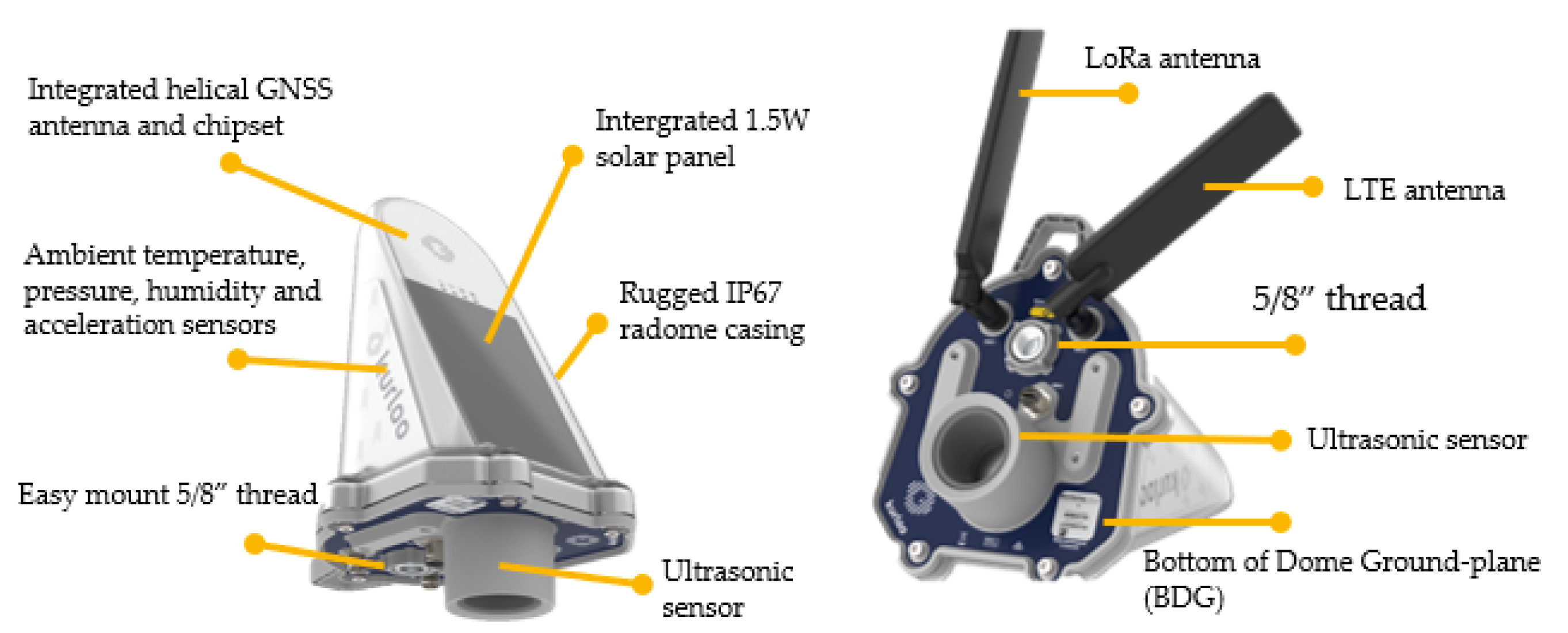
Figure 2.
The ultrasonic sensor measurement and ambient temperature example. (a) ultrasonic sensor epoch readings every 30 minutes. (b) ambient temperature recordings every 30 minutes. (c) scatter plot of ultrasonic sensor and temperature epoch measurement. (d) scatter plot of ultrasonic sensor and temperature average daily measurement.
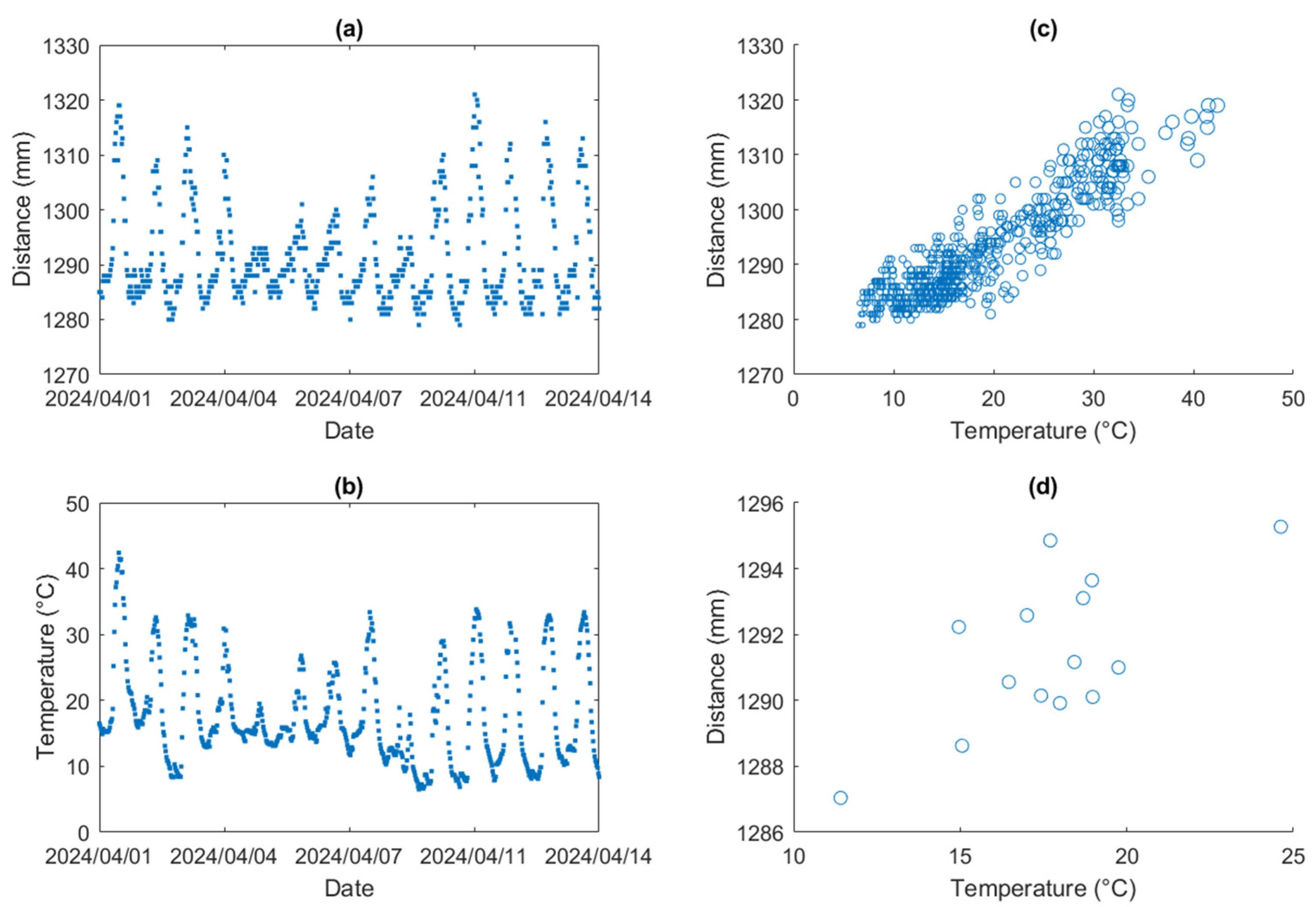
Figure 3.
Definition of axis and tilt angles in the device.
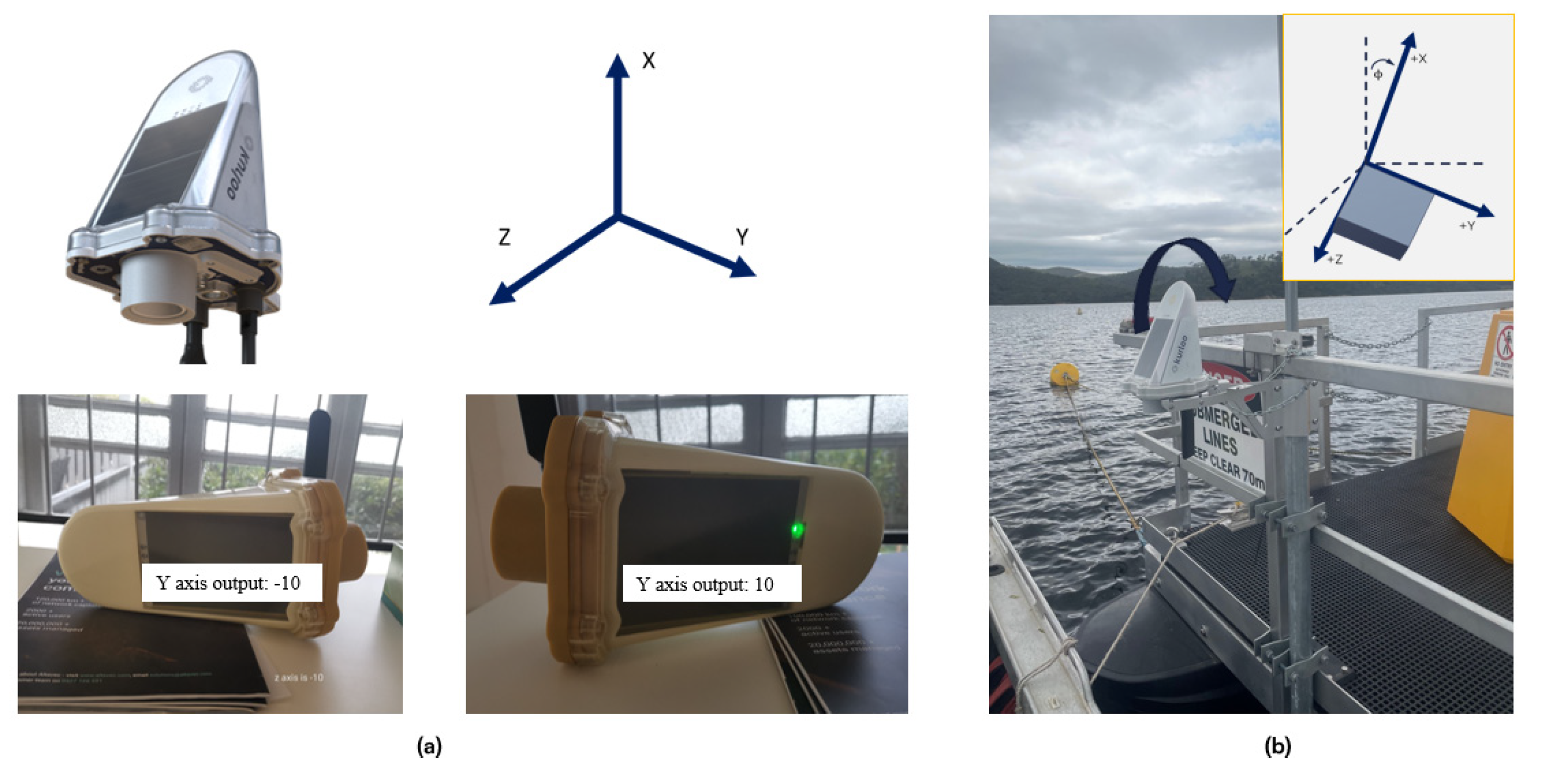
Figure 4.
Pontoon tilting angle variations.
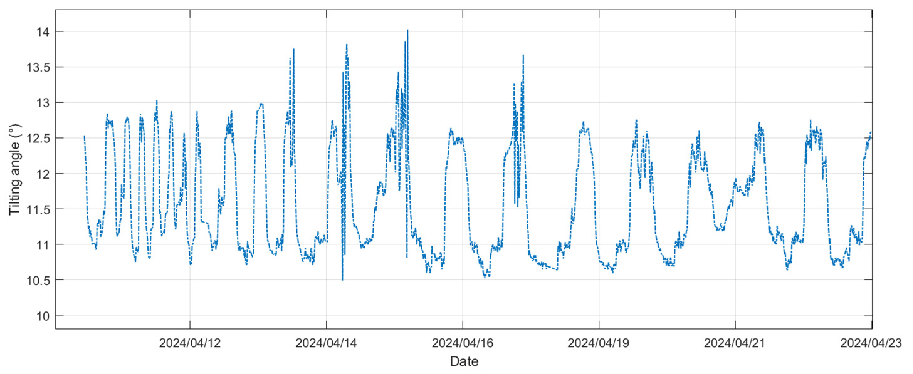
Figure 5.
Schematic of pontoon tilting impact on height.
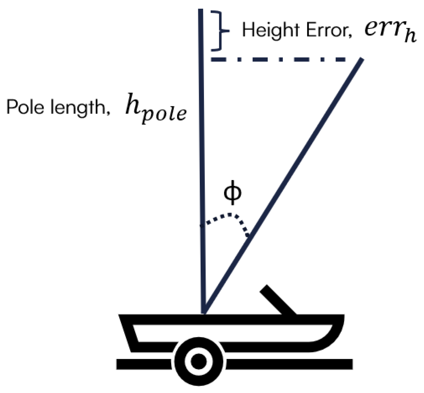
Figure 6.
Experimental set-up on the CSIRO Dark-water Inland Observatory Network’s pontoon at Googong reservoir (photo credit: D. Culvenor and G. Kerrisk).
Figure 6.
Experimental set-up on the CSIRO Dark-water Inland Observatory Network’s pontoon at Googong reservoir (photo credit: D. Culvenor and G. Kerrisk).
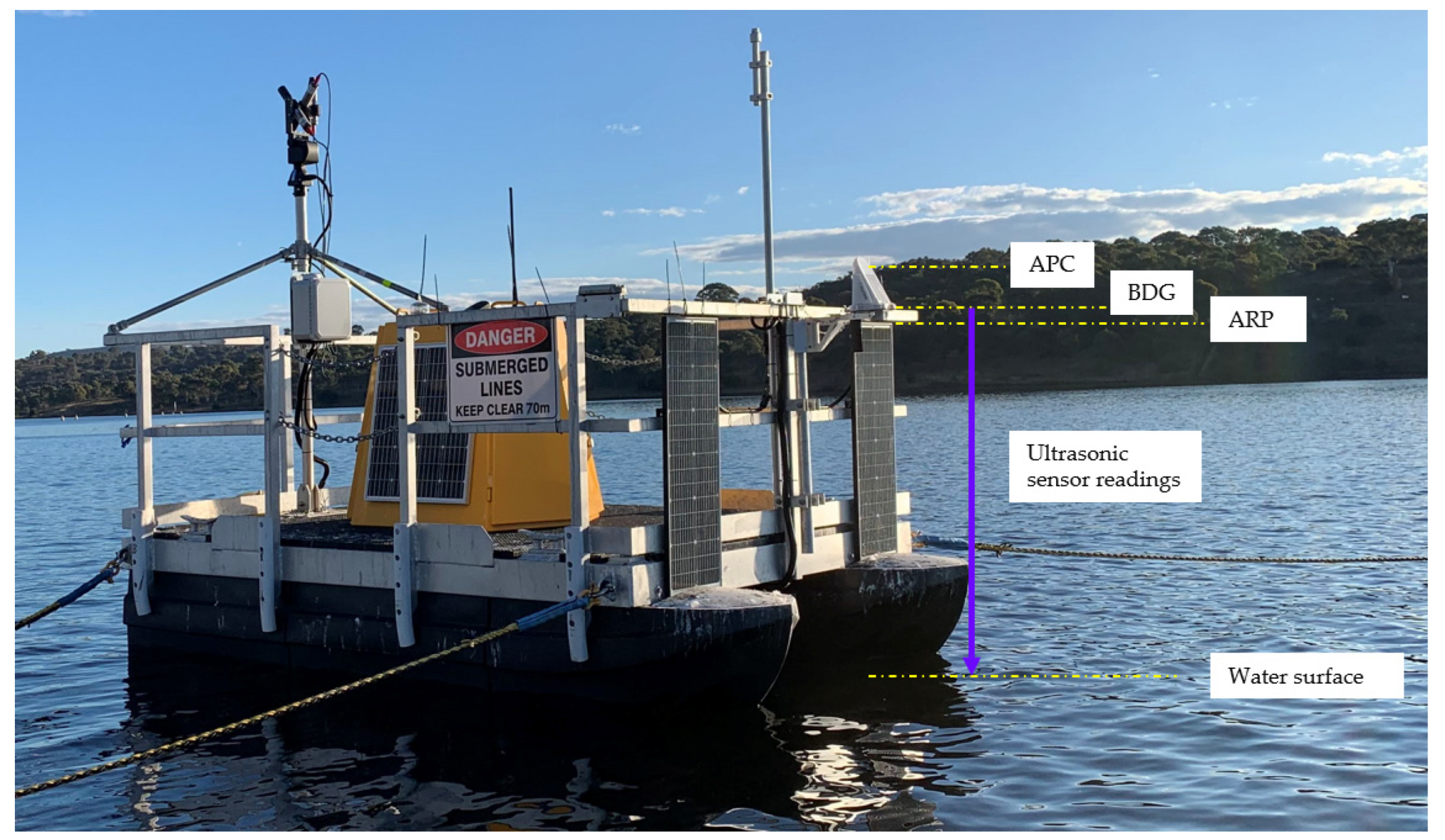
Figure 7.
Two devices in the experiment. (a) F043 stable base station; (b) F044 floating station.
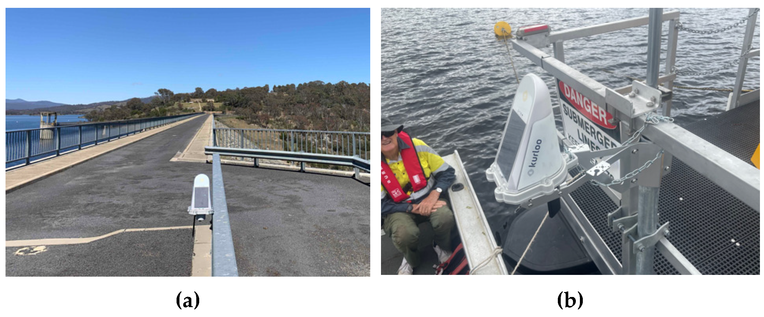
Figure 8.
Icon Water Googong reservoir WSE data from 1/Feb/2024 to 30/May/2024. (a): raw data with 10 minutes interval, 24-hour and 6-hour average data; (b): WSE variation range in 24 hours and 6 hours; (c): difference between the 24-hour and 6-hour average data.
Figure 8.
Icon Water Googong reservoir WSE data from 1/Feb/2024 to 30/May/2024. (a): raw data with 10 minutes interval, 24-hour and 6-hour average data; (b): WSE variation range in 24 hours and 6 hours; (c): difference between the 24-hour and 6-hour average data.
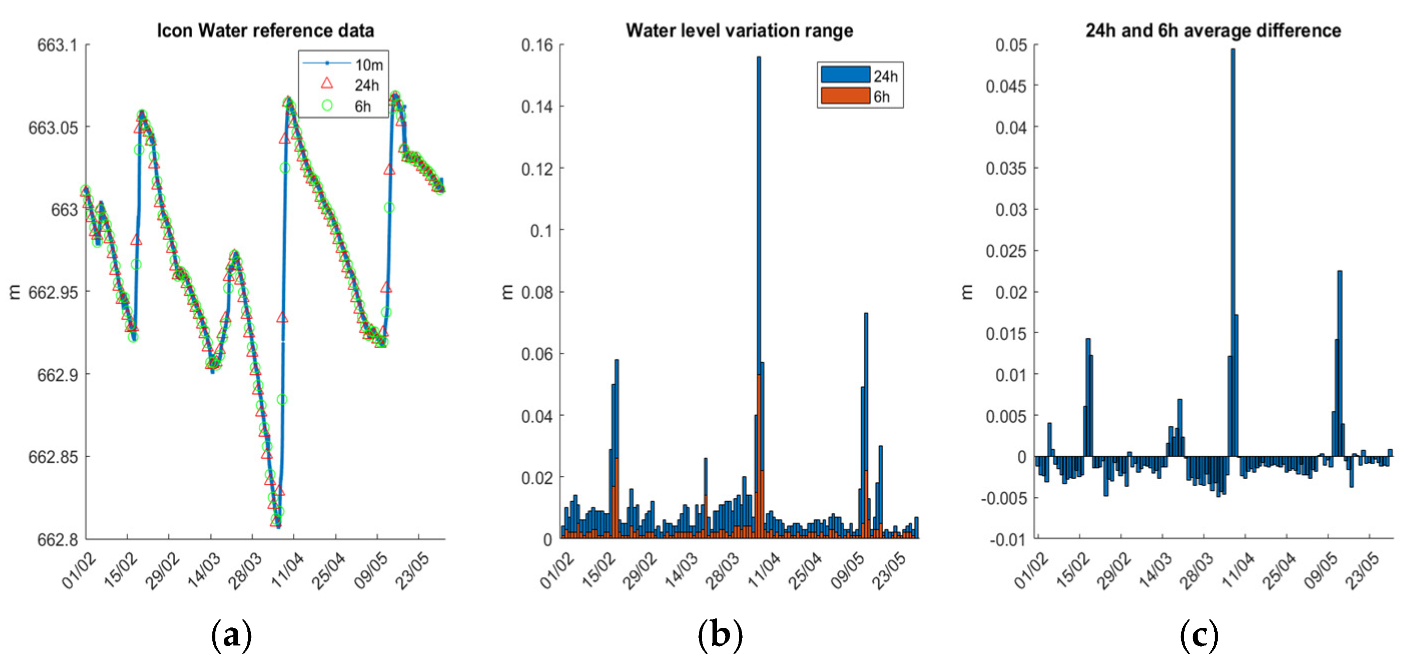
Figure 9.
Ultrasonic sensor readings from 1/Feb/2024 to 30/May/2024. (a) Raw and smoothed data time series. (b) Histogram of raw data and (c) histogram of smoothed data.
Figure 9.
Ultrasonic sensor readings from 1/Feb/2024 to 30/May/2024. (a) Raw and smoothed data time series. (b) Histogram of raw data and (c) histogram of smoothed data.
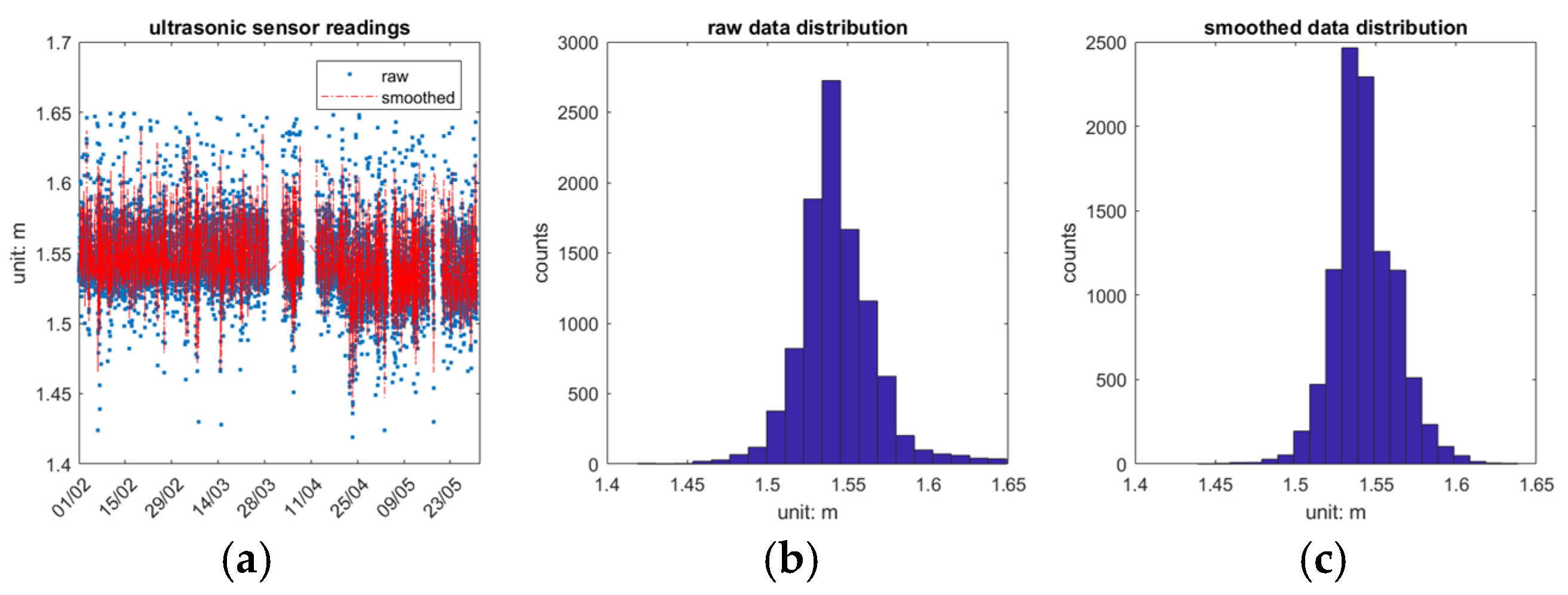
Figure 10.
The ultrasonic sensor daily average measurement in the experiment.
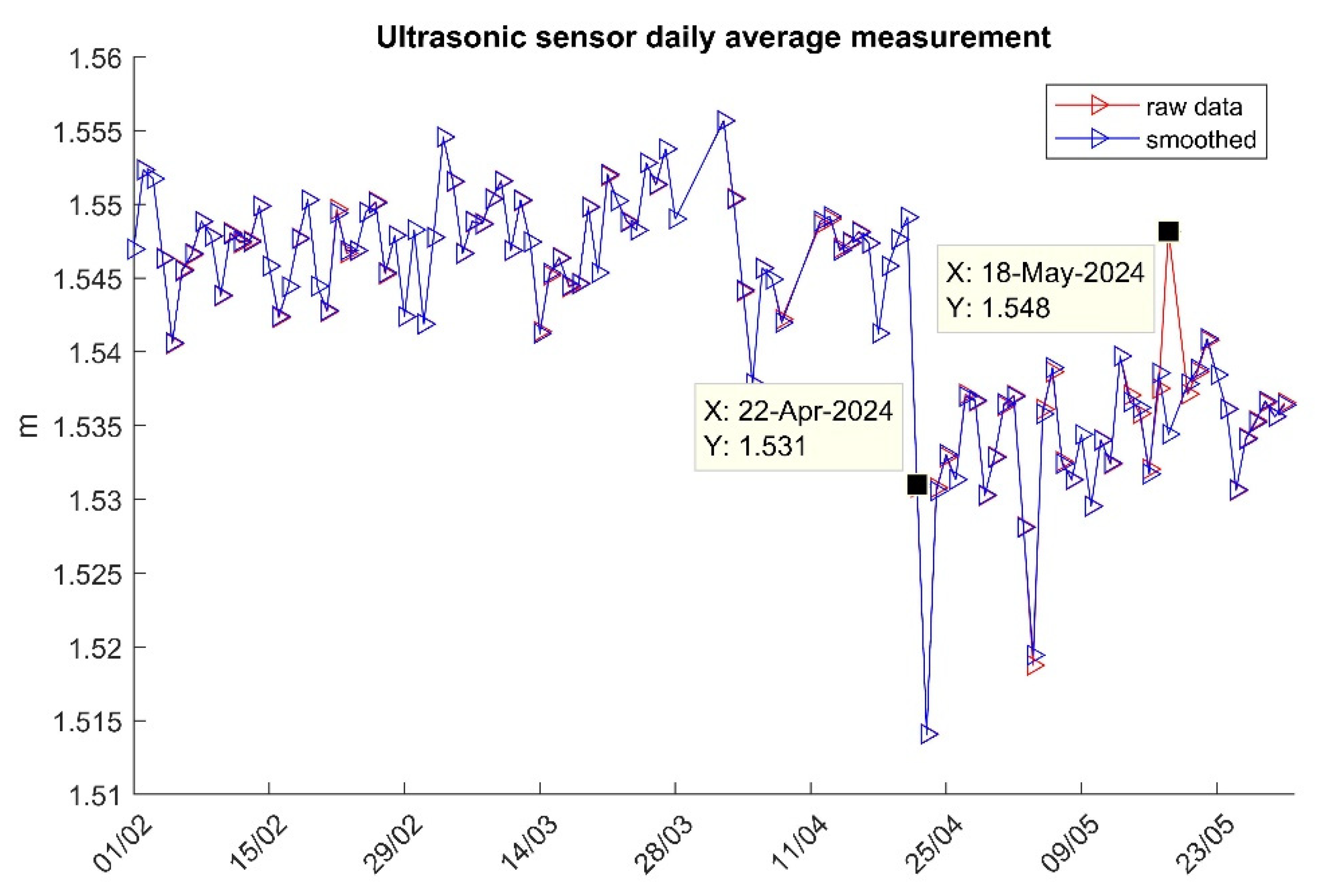
Figure 11.
Datum offset estimation with epoch and daily data for 2 weeks.
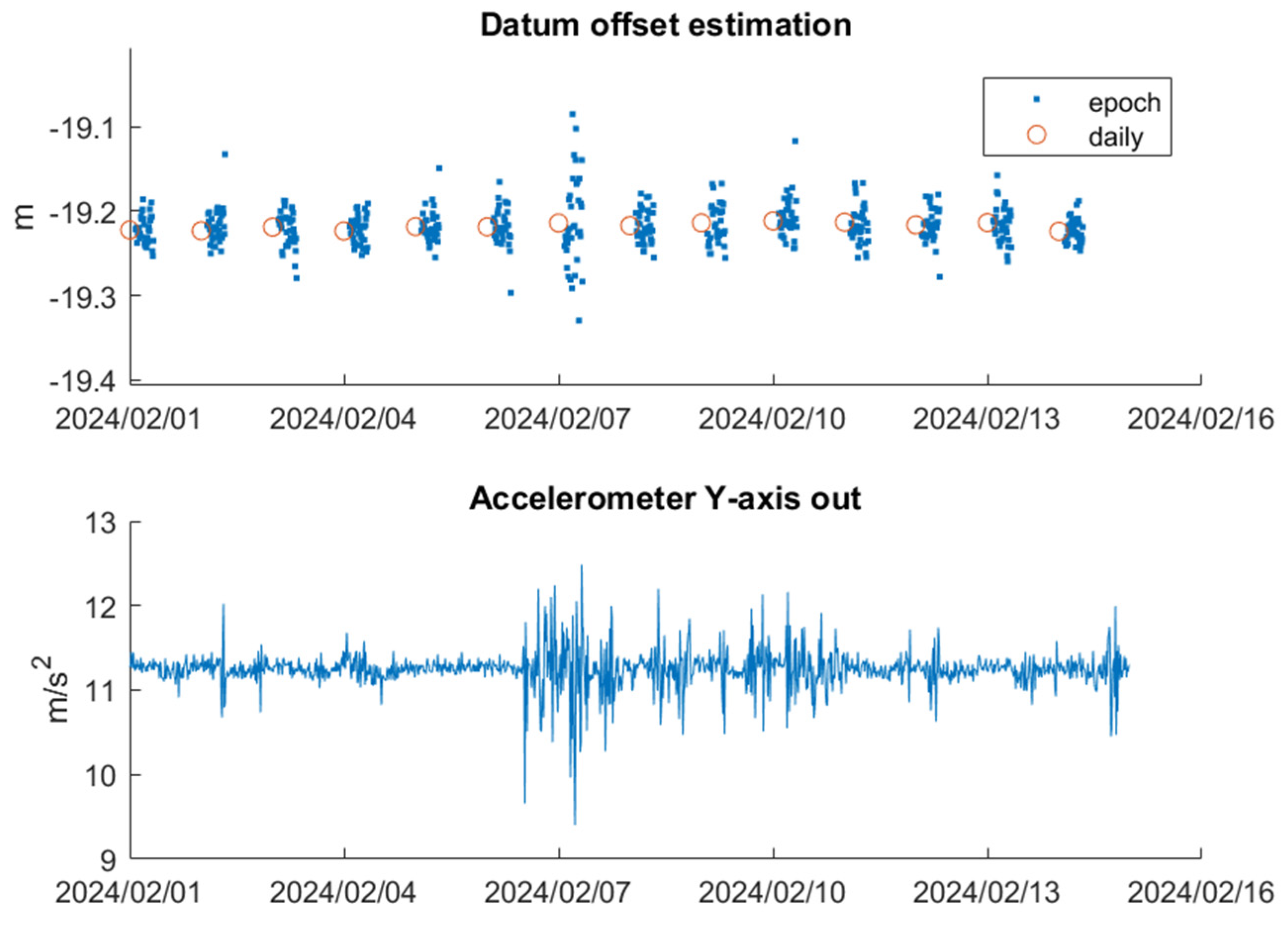
Figure 12.
System epoch solutions. (a): Reference, “orig”, and “high”. (b): the difference between Reference and “orig”, “high”. (c): the histogram of the difference distribution.
Figure 12.
System epoch solutions. (a): Reference, “orig”, and “high”. (b): the difference between Reference and “orig”, “high”. (c): the histogram of the difference distribution.
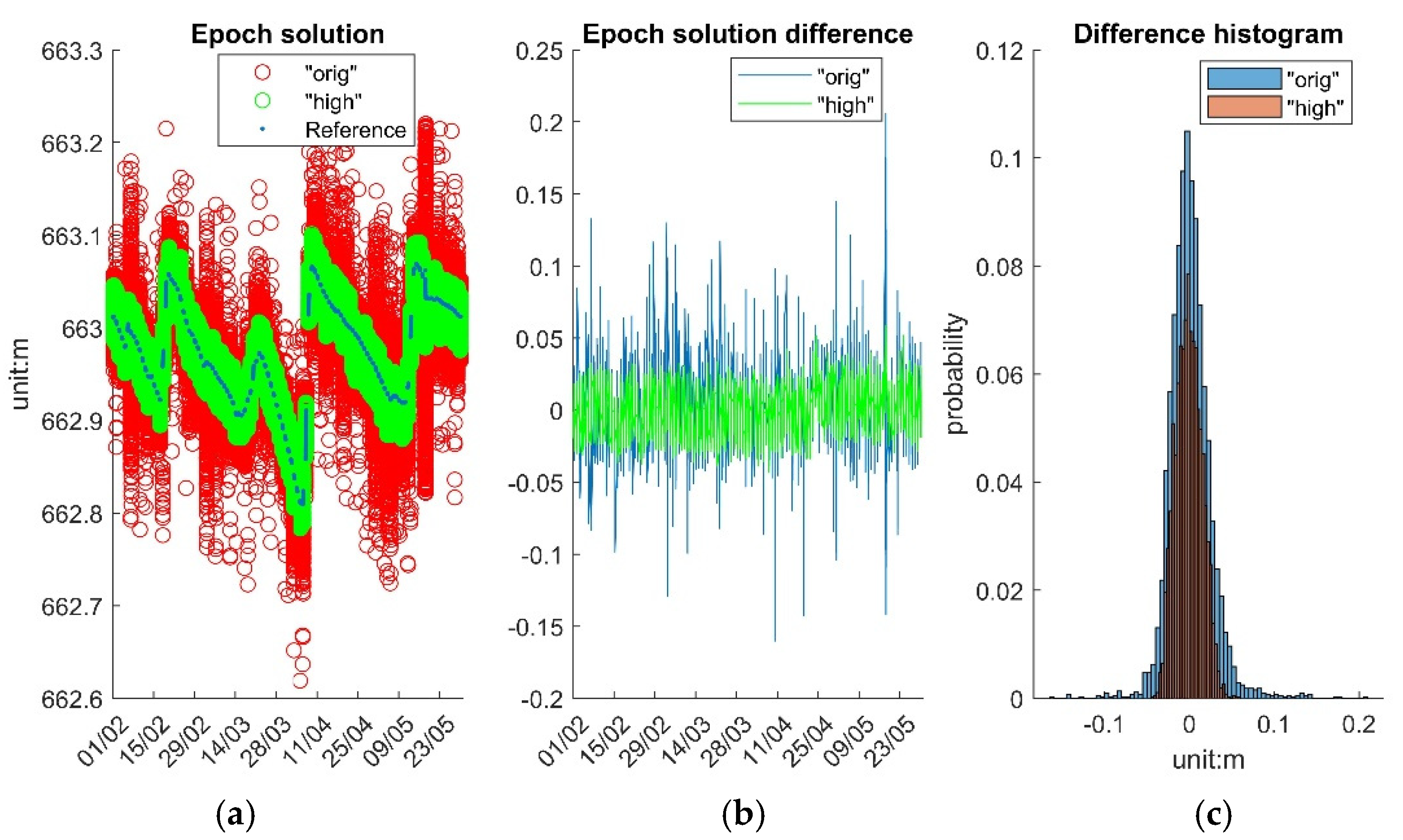
Figure 13.
System daily solution. (a): Reference, “orig”, and “high”. (b): the difference between Reference and “orig”, “high”. (c): the histogram of the difference distribution.
Figure 13.
System daily solution. (a): Reference, “orig”, and “high”. (b): the difference between Reference and “orig”, “high”. (c): the histogram of the difference distribution.
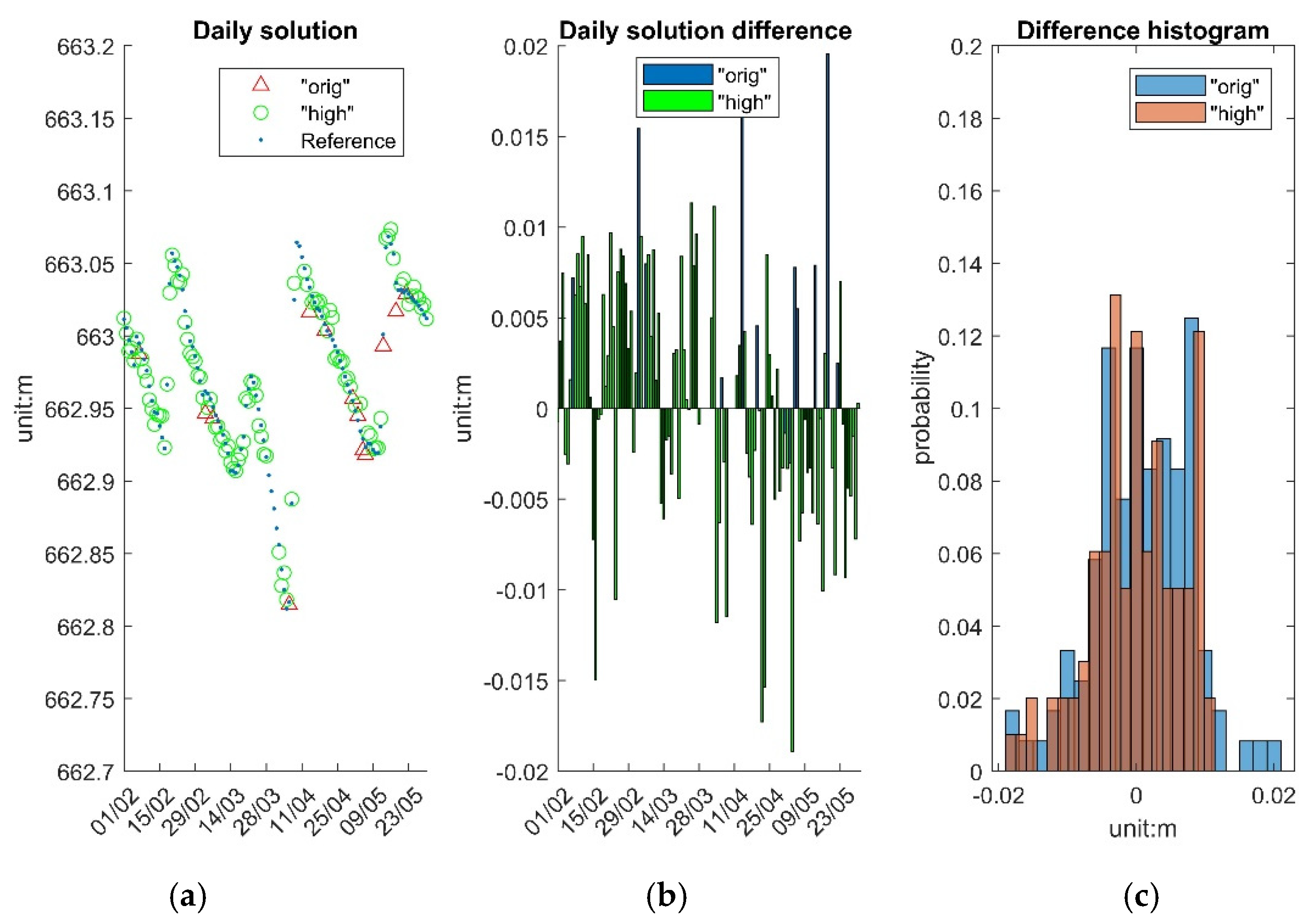
Figure 14.
Site rainfall data and System daily solution QC flag. Top: Daily rainfall data. Middle: System QC flag. Bottom: Absolute difference between System and reference data.
Figure 14.
Site rainfall data and System daily solution QC flag. Top: Daily rainfall data. Middle: System QC flag. Bottom: Absolute difference between System and reference data.
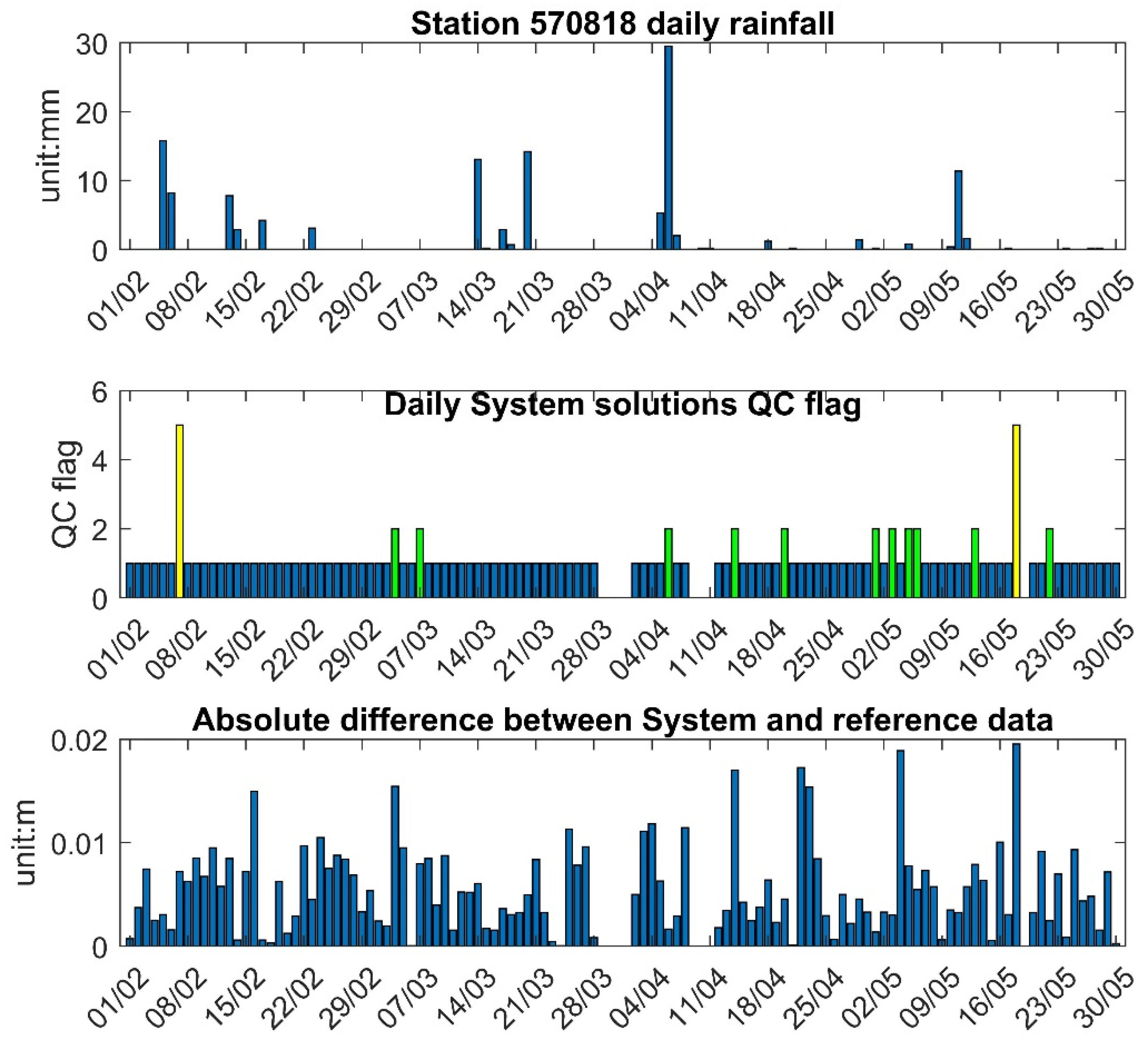
Figure 15.
Device APC 2D variations. (a): east and north positioning; (b): 2D tracking.
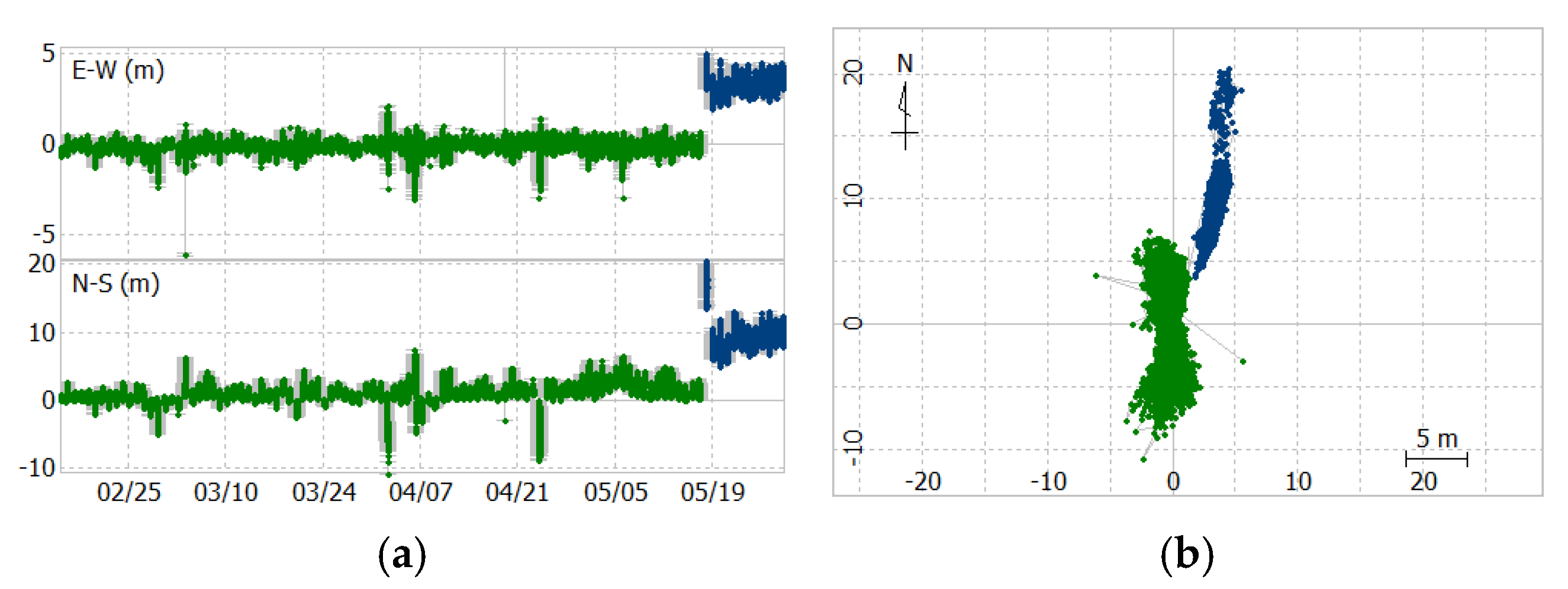

Table 1.
Ultrasonic sensor calibration testing values.
| Test ID | BDG to timber board (m) | Ultrasonic sensor reading (m) | Difference (m) |
| 1 | 1.005 | 1.017 | 0.012 |
| 2 | 0.793 | 0.804 | 0.011 |
| 3 | 0.459 | 0.469 | 0.010 |
| 4 | 1.068 | 1.077 | 0.009 |
| Average: | 0.011 | ||
Table 2.
The system applied RTKLIB main configuration parameters.
| RTKLIB Parameters | Settings |
|---|---|
| Positioning mode | Kinematic |
| Interval | 15 seconds |
| Filter type | Combined |
| Elevation mask | 20 degrees |
| Satellite Ephemeris | Broadcast |
| Ionospheric correction | Broadcast |
| Tropospheric correction | Saastamoinen |
| Ambiguity Resolution | GPS Fix and Hold |
| Ambiguity Ratio | 4 |
| Constellations | GPS, Galileo, BDS and QZSS |
Table 3.
WSE estimation error budget.
| Symbol | Description | Approximate value (m) |
|---|---|---|
| GNSS kinematic positioning error | 0.015 | |
| Ultrasonic sensor measurement error | 0.020 | |
| Tilting error | 0.005 | |
| Other unknown error | 0.010 | |
| WSE estimation error | 0.027 |
Table 4.
Descriptive statistics for the WSE data provided by Icon Water (unit: m).
| Description | Mean | Std | Min | Max | Range |
| WSE variation range in 24h | 0.011 | 0.018 | 0.001 | 0.156 | 0.155 |
| WSE variation range in 6h | 0.003 | 0.006 | 0.000 | 0.053 | 0.053 |
| Difference of 24h and 6h average | 0.000 | 0.006 | -0.005 | 0.050 | 0.055 |
Table 5.
Maximum, minimum, mean, median and std values of ultrasonic sensor readings (unit: m).
| Data type | Max. | Min. | Mean | Median | Std. | Range |
| raw data | 1.649 | 1.419 | 1.543 | 1.541 | 0.024 | 0.230 |
| smoothed data | 1.639 | 1.439 | 1.543 | 1.541 | 0.019 | 0.200 |
Table 6.
Datum Offset / Correction Estimation (unit: m).
| Observed 2 weeks | Observed 4 weeks | |||||
| Data type | Mean | Std | Range | Mean | Std | Range |
| Epoch | -19.217 | 0.028 | 0.266 | -19.219 | 0.027 | 0.266 |
| Daily | -19.218 | 0.004 | 0.013 | -19.219 | 0.006 | 0.025 |
Table 7.
Overall testing period System Accuracy Performance (unit: m).
| ”orig” | “high” | |||||||
|---|---|---|---|---|---|---|---|---|
| Data type | Mean | Std | Range | Max | Mean | Std | Range | Max |
| Epoch | -0.006 | 0.028 | 0.354 | 0.198 | -0.007 | 0.020 | 0.167 | 0.086 |
| Daily | 0.001 | 0.007 | 0.038 | 0.019 | 0.000 | 0.007 | 0.030 | 0.019 |
Disclaimer/Publisher’s Note: The statements, opinions and data contained in all publications are solely those of the individual author(s) and contributor(s) and not of MDPI and/or the editor(s). MDPI and/or the editor(s) disclaim responsibility for any injury to people or property resulting from any ideas, methods, instructions or products referred to in the content. |
© 2025 by the authors. Licensee MDPI, Basel, Switzerland. This article is an open access article distributed under the terms and conditions of the Creative Commons Attribution (CC BY) license (http://creativecommons.org/licenses/by/4.0/).
Copyright: This open access article is published under a Creative Commons CC BY 4.0 license, which permit the free download, distribution, and reuse, provided that the author and preprint are cited in any reuse.


