
Submitted:
23 April 2025
Posted:
23 April 2025
You are already at the latest version
Abstract
Across the Philippines, rapid urban expansion has led to significant shifts in land use, population distribution, and environmental conditions. While urbanization presents economic opportunities, it also intensifies challenges such as declining green spaces, including increasing urban temperatures and vulnerability to climate-related risks. This study examines the environmental transformation of Puerto Princesa City, Palawan, from 2014 to 2022, analyzing land cover change, population growth, and their broader ecological and social implications. Data analysis revealed that Puerto Princesa City underwent significant land use and land cover changes, with built-up areas nearly doubling from 34.4 km² to 67.7 km², driven by population growth and urban expansion. The transformation of open spaces into built-up zones was most evident in urban peripheries, while rural barangays exhibited varied trends, including expansion, stagnation, and even forest cover increase. The analysis of LST correlations with vegetation and built-up areas revealed a low correlation between LST and NDVI but a moderate to high correlation between LST and NDBI, suggesting that urbanization contributes to increased temperatures. OLS regression indicated strong relationships between environmental parameters and population density, with NDVI decreasing and both NDBI and LST increasing as population density rose. The SUHI effect fluctuated, with an unusual drop in 2016 possibly due to the El Niño-induced vegetation drying, which increased rural temperatures more rapidly than urban ones. By 2022, continued urbanization and land conversion sustained higher SUHI values, underscoring the environmental impact of rapid development.
Keywords:
Urbanization
; Urban Heat Island
; Land Cover Change
; Philippines
1. Introduction
The transition from predominantly rural to urban societies has been both a major driver and outcome of the rapid social and economic transformation witnessed across Asia in recent decades (Hugo, 2019). In the Philippines, studies reveal a significant increase in built-up areas and population, highlighted by enduring urbanization processes that have permanently reshaped the country’s landscape (Santillan and Heipke, 2024). These changes bring significant opportunities for progress but also present persistent environmental and socioeconomic challenges that require careful planning and management (Ahmad et al., 2018; Patra et al., 2018).
Rapid urbanization leads to several adverse effects, including land use change, flood risk, pollution, and the urban heat island (UHI) phenomenon. Land use change involves the conversion of natural landscapes into urban or industrial areas, resulting in habitat loss, ecosystem disruption, and increased surface runoff (Choudhury et al. 2019). Subsequently, UHI indicates built-up areas that have higher atmospheric and land surface temperature (LST) than the surrounding rural areas (Landsberg, 1981). Many highly urbanized and high-density cities across Asia noted declining canopy cover, increasing LST, and signs of the UHI phenomenon (Rana et al., 2024; Halder et al., 2021). These phenomena have severe adverse implications for public health, energy consumption, and overall environmental sustainability (Dong et al., 2014; Nguyen et al., 2019).
Similar to many cities in the region, Puerto Princesa, the administrative capital of the Province of Palawan in the southwestern Philippines, experiences the complex impacts of urbanization. These include a steadily growing population and expanding built-up areas alongside the persistent need to address challenges related to sustainable development, urban management, and environmental preservation. With the observable expansion of built-up areas and the corresponding decline in green spaces within the city’s urban zones, managing increasing urban temperatures in the city, especially during dry months, is becoming a local governance concern.
This study examined the urban development trends in Puerto Princesa City over an eight-year period from 2014 to 2022, focusing on their environmental implications. Specifically, it analyzed the evolution of land cover and population distribution across the city’s barangays and its connection to the intensification of the Urban Heat Island (UHI) phenomenon. By exploring these dynamics, the study intends to provide a comprehensive understanding of how urbanization has reshaped the city’s landscape, highlighting key patterns of land-use change and their potential impact on local climate, biodiversity, and socioeconomic development.
2. Materials and Methods
2.1. The Study Area
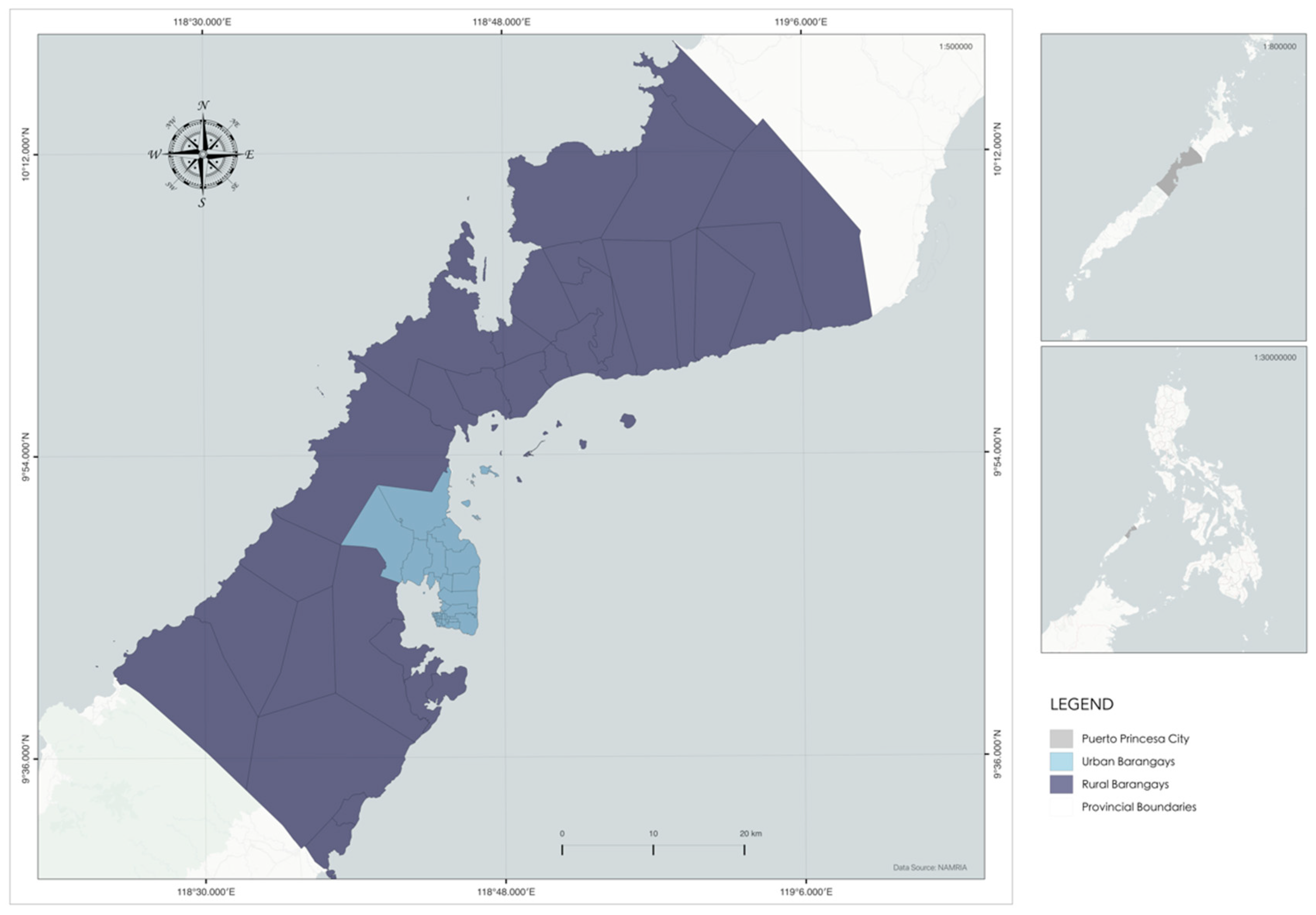
Puerto Princesa City, a highly urbanized city (HUC) centrally located on the island of Palawan, despite functioning as a separate political entity, is the capital of the Province of Palawan. The city spans a total land area of 219,339.40 hectares, making it the second-largest city in the Philippines by land area. It is divided into 66 barangays, comprising 35 urban and 31 rural barangays. The urban barangays cover 14,716 hectares, representing 6.71% of the city’s total land area, while the rural barangays collectively account for approximately 204,623 hectares, or 93.29% of the total.
Figure 1.
Location map of the study area.
Puerto Princesa City's population reached 307,079 in the 2020 national census, marking a 20.37% increase from 2015. This growth reflects a steady annual rate of 3.98%, outpacing neighboring provinces. Notably, the city's rural barangays experienced an even higher annual growth rate of 4.29%, suggesting a gradual shift toward urbanization. Despite this trend, the majority of the population, approximately 75.23%, remains concentrated in the urban districts.
2.2. Data Sourcing
This study utilized open-access sociodemographic and spatial data to achieve its key objectives. Secondary data were sourced from the Philippine Statistics Authority (PSA) census to analyze the city's population trends. The city’s land cover data were generated using Landsat 8 images downloaded from USGS Earth Explorer. Due to topography and climatic factors in the study area, it is difficult to collect images that are free of clouds and other atmospheric disturbances, necessitating the removal of the pixels containing the aforementioned elements and filling them with clear pixels from images taken in the same year. Additionally, masked pixels were also manually reclassified by comparing them with historical imagery on Google Earth Engine. On the other hand, masked versions of Landsat 8 images detailed in Table 1 were employed to analyze the Normalized Difference Built-up Index (NDBI), Normalized Difference Vegetation Index (NDVI), Land Surface Temperature (LST), and Urban Heat Island (UHI) effects. These Landsat 8 images were chosen as they have the least amount of cloud cover over the area of interest.
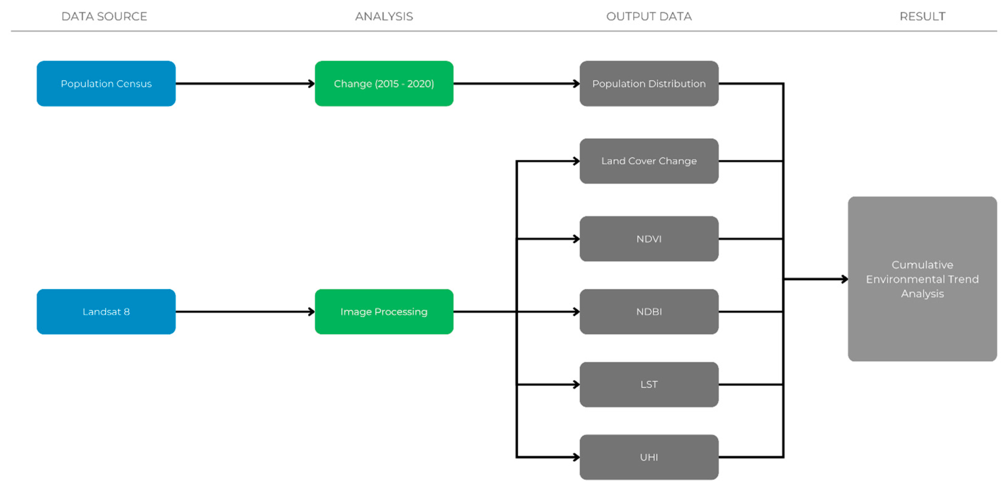
Figure 2.
The study flowchart modified from Nguyen et al., 2019.
2.3. Geospatial Analysis
The framework utilized for this study integrates multiple data sources, analytical methods, and environmental indicators to assess landscape changes over time. The study used indicators including population distribution and land cover change from census and land cover assessments, while remote sensing techniques generate indices such as the Normalized Difference Vegetation Index (NDVI) for vegetation health, Normalized Difference Built-up Index (NDBI) for urban expansion, Land Surface Temperature (LST) for surface heat distribution, and Urban Heat Island (UHI) effect to assess temperature variations associated with urbanization. The results of these analyses contribute to a Cumulative Environmental Trend Analysis, providing a comprehensive assessment of the interactions between population dynamics, land cover change, and urban-induced thermal variations.
Landsat 8 data was used to retrieve land surface temperature (LST) and related indices. Band 10 (Thermal Infrared 1) was utilized for LST estimation, while Bands 4 (Red) and 5 (Near Infrared) were combined for NDVI calculation. Additionally, Bands 5 (Near Infrared) and 6 (Shortwave Infrared 1) were used to compute the NDBI. Landsat 8 TIRS Band 10 was used to retrieve land surface temperature (LST) through a three-step process: (a) converting digital numbers (DN) to top-of-atmosphere (TOA) radiance using radiometric rescaling coefficients from the metadata file, (b) transforming spectral radiance into TOA brightness temperature, and (c) deriving LST from brightness temperature using an emissivity correction approach (Alabi et al., 2021; USGS, 2019).
2.4. Statistical Analysis
2.4.1. Environmental Parameters Scatter Plots and Correlations
Scatter plots were generated from extracted pixel values of the generated LST, NDVI, and NDBI maps to visualize the relationship between these indices. Pearson r correlation coefficients were then calculated using the python scipy package to examine the relationship of LST with NDVI and NDBI.
The Pearson r correlation coefficient was calculated using the following equation,
where r is the correlation coefficient, is the ith entry in the LST masked pixel data values, is either the ith entry in the NDBI or NDVI masked pixel data values, and are the mean values of the x and y data, respectively.
2.4.2. Environmental Parameters with Population Density Multi-Linear Regression
The population density was determined for each of the 66 barangays. Barangay boundaries were used to isolate clusters of pixels corresponding to each barangay. The mean values of LST, NDVI, and NDBI were then calculated for each cluster, generating a table of population density versus environmental parameters (LST, NDVI, and NDBI). The relationship between each environmental parameter and population density was analyzed using an Ordinary Least Squares (OLS) regression model in Python with the statsmodels package.
In the Ordinary Least Square (OLS) regression model, the environmental parameters were assumed to be linearly dependent on the logarithm of the population, that is,
where the environmental parameters are Y = {LST, NDVI, LST}, P is the population, the coefficients to be optimized in the model are , is the error term, and the dummy variables {D1, D2, D3} have value 1 or 0 depending on which year the Y and P belong to. Year 2014 data have all dummy variables set to zero, year 2016 have dummy variables D1 set to 1 while the others are zero, year 2020 have dummy variables D2 set to 1 while the others are zero, and year 2022 have dummy variables D3 set to 1 while the others are zero.
The optimized coefficients determined in the OLS is given by the following equation,
where is the column vector of coefficients, is the matrix with columns as values of the independent variables, and is the column vector of observed environmental parameter values.
The R-squared () coefficient measures how well the regression model explains the variability in the dependent variable and is given by the following equation,
where are the observed environmental parameter values, are the model-predicted environmental parameter values, and is the mean of the observed environmental parameter values.
3. Results
3.1. Population Trends
The population density and population change data from 2015 to 2020 across the rural and urban barangays of Puerto Princesa City show notable demographic trends. Based on the census data from the Philippine Statistics Authority (PSA), rural areas generally exhibited a higher population growth rate than urban areas, with a 14.79% average change across all rural barangays. This trend suggests a shift in population distribution, potentially indicating rural development, expansion of residential areas, or increasing economic opportunities in certain rural barangays. Among the rural barangays, Cabayugan recorded the highest population density increase of 210%, with its population growing from 1,212 in 2015 to 3,754 in 2020, as seen in Figure 4. Conversely, some rural barangays experienced a notable population decline. Binduyan, for instance, recorded a 71.61% decrease in population from 5,350 in 2015 to 1,519 in 2020, resulting in a drastic reduction in population density from 62 to 18 individuals/km².
Figure 3.
Population density per km2 in barangays of Puerto Princesa City in 2015 and 2020 (Data Source: Philippine Statistics Authority).
Figure 3.
Population density per km2 in barangays of Puerto Princesa City in 2015 and 2020 (Data Source: Philippine Statistics Authority).
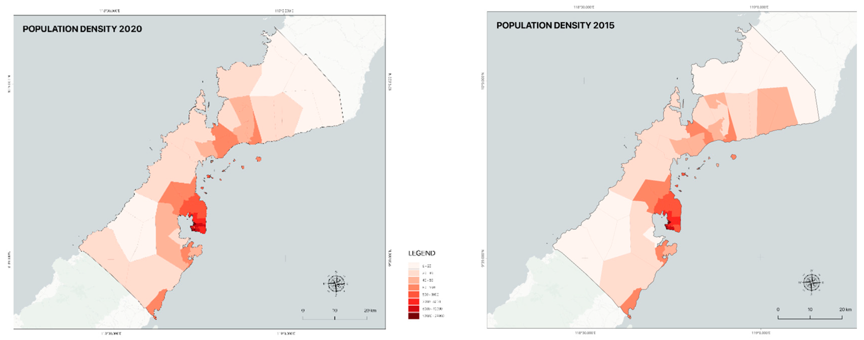
In urban areas, population changes were less pronounced, with an average of only 1.25% change in density. Figure 4 highlights the barangays of San Manuel and San Jose, which recorded some of the highest population increases, with growth rates of 47.95% and 35.86%, respectively. A striking observation in the dataset is the emergence of highly congested urban barangays, notably Pagkakaisa, where the population density increased to approximately 39,267 individuals/km², the highest in the city. Other densely populated urban barangays include Liwanag (21,948 individuals/km²) and Masikap (18,980 individuals/km²). Additionally, the urban barangay of San Pedro showed a 17.29% increase in population density, from 3,418 to 4,009 individuals/km², which may indicate ongoing urban development and housing expansion in the area.
3.2. Land Cover Change
The land cover maps generated in Figure 5 show the different land cover types considered in this study: water, developed, sparse vegetation, forest, and mixed vegetation. The transition matrices for the consecutive years were calculated and summarized in Table 2, Table 3 and Table 4, revealing notable changes over time. Mixed vegetation experienced significant fluctuations. From 2014 to 2016, it declined markedly from 688.1 km² to 561.8 km². However, the years 2016 to 2020 saw a recovery, with the area increasing from 516.7 km² to 655.1 km². In contrast, the period from 2020 to 2022 exhibited minimal change, with mixed vegetation slightly decreasing from 655.1 km² to 646.2 km².
Water bodies showed a declining trend from 2014 to 2016, shrinking from 21.9 km² to 14.8 km². This was followed by a modest increase from 15.2 km² to 18.5 km² between 2016 and 2020. Notably, from 2020 to 2022, the water-covered area nearly doubled, rising from 18.4 km² to 32.1 km².
Forest cover remained relatively stable, with minor fluctuations throughout the study period. It increased slightly from 1365.5 km² to 1441.6 km² between 2014 and 2016, then decreased to 1375.2 km² by 2020, and finally rose again to 1404.5 km² by 2022. Sparse vegetation exhibited a contrasting trend, with a notable increase from 81.8 km² to 113.9 km² between 2014 and 2016, followed by a gradual decline to 82.8 km² in 2020 and a further reduction to 40.0 km² in 2022. Developed areas consistently expanded throughout the study period. From 2014 to 2016, the area increased from 34.4 km² to 59.6 km², followed by a slight rise to 61.1 km² by 2020, and continued growth to 67.7 km² by 2022.
3.3. NDBI and NDVI Values
The NDVI values reveal a clear contrast in vegetation cover between urban and rural barangays in Puerto Princesa City. Urban barangays generally have lower NDVI values (0.1 to 0.3) due to high population density and land development, with minimal or decreasing trends from 2014 to 2022. The highest NDVI values in urban areas, such as Sicsican and Sta. Lourdes reached around 0.480, while the most densely populated barangays like Pagkakaisa, Liwanag, and Bagong Silang rarely exceeded 0.2. In contrast, rural barangays with less infrastructure development exhibit higher NDVI values (0.4 to 0.5) and stable or increasing trends, with Napsan, Binduyan, and New Panggangan reaching as high as 0.521 in 2020.
Figure 6.
Maps representing mean NDVI values across the barangays of Puerto Princesa City from 2014 to 2022.
Figure 6.
Maps representing mean NDVI values across the barangays of Puerto Princesa City from 2014 to 2022.
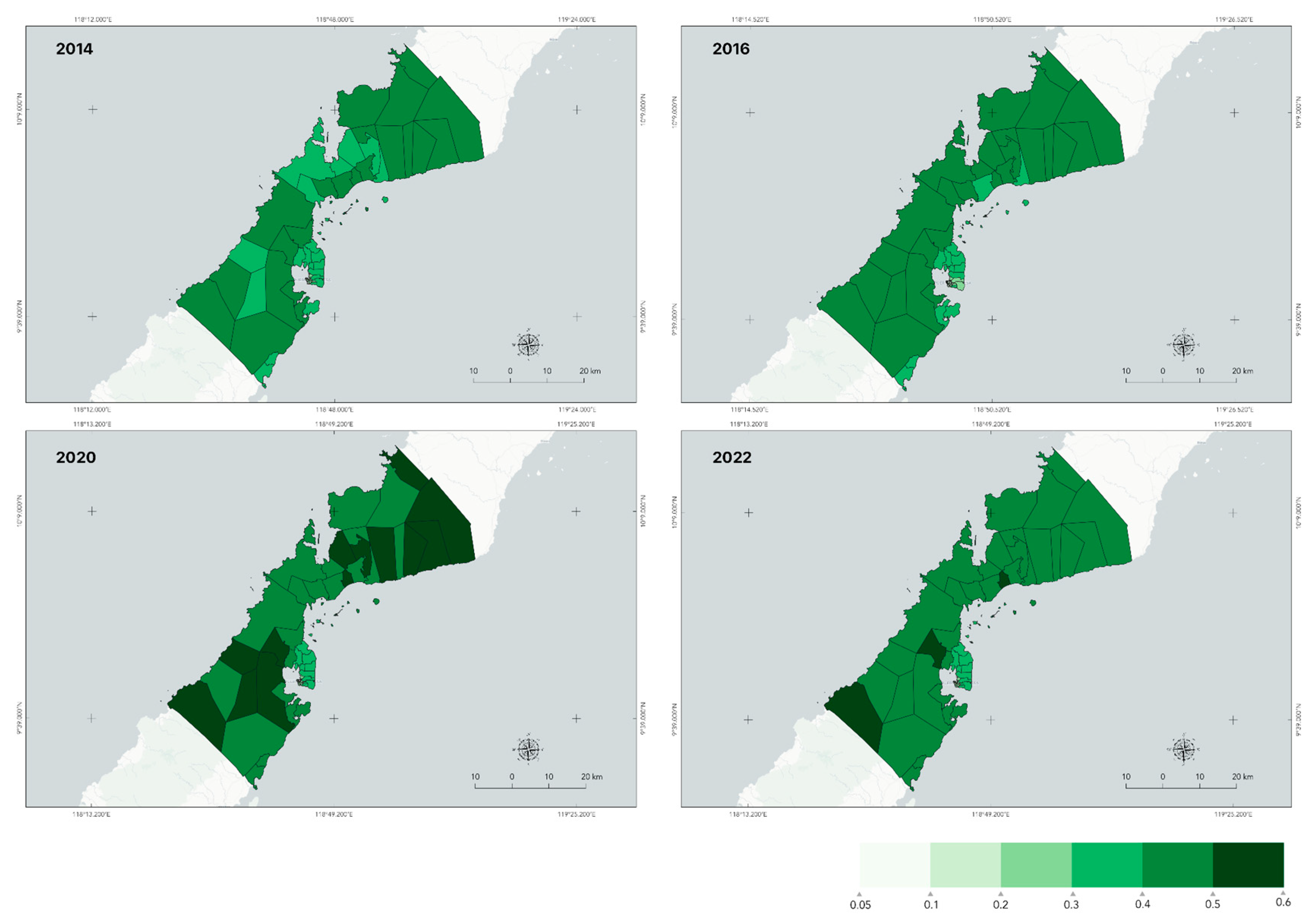
Figure 7.
Mean NDVI values across the barangays of Puerto Princesa City arranged from highest (left) to lowest (right) density.
Figure 7.
Mean NDVI values across the barangays of Puerto Princesa City arranged from highest (left) to lowest (right) density.
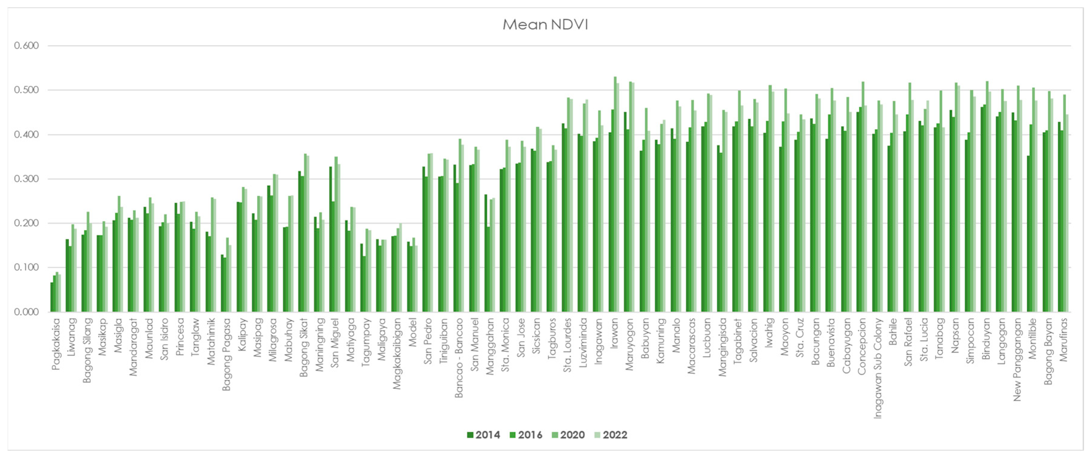
Figure 8.
Maps representing mean NDBI values across the barangays of Puerto Princesa City from 2014 to 2022.
Figure 8.
Maps representing mean NDBI values across the barangays of Puerto Princesa City from 2014 to 2022.
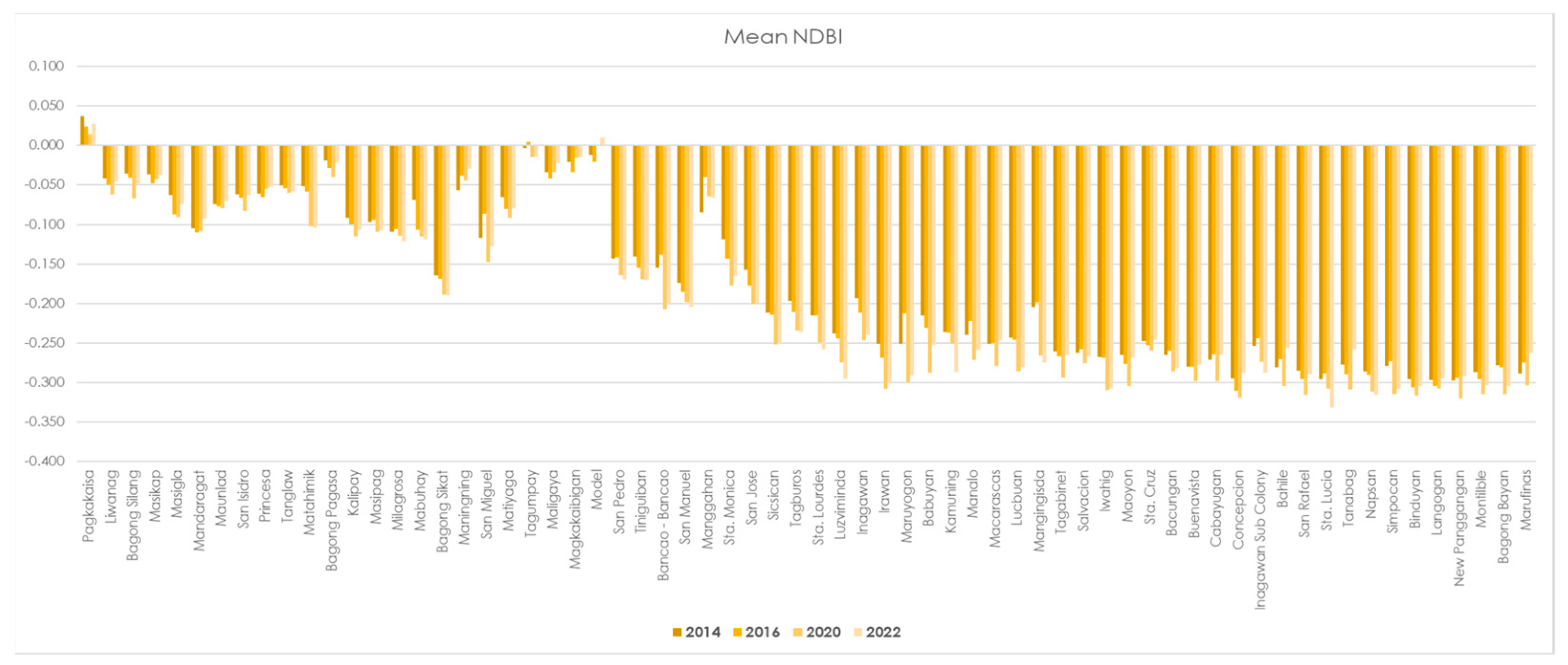
The NDBI values show a general decline from 2014 to 2022, indicating either a reduction in built-up areas or an increase in vegetation cover. High density urban barangays, such as Pagkakaisa, Liwanag, and Bagong Silang, exhibited consistently low NDBI values, reflecting limited infrastructure expansion or increased green space. Moderate density barangays like Mandaragat and San Pedro also showed declining NDBI values, suggesting efforts in vegetation restoration. In rural barangays, such as Luzviminda, Inagawan, and Irawan, NDBI values were consistently negative, indicating minimal built-up areas and dominant natural vegetation. This overall trend suggests gradual improvements in urban greening or slower infrastructure growth, particularly in urban barangays.
Figure 9.
Mean NDBI values across the barangays of Puerto Princesa City arranged from highest (left) to lowest (right) density.
Figure 9.
Mean NDBI values across the barangays of Puerto Princesa City arranged from highest (left) to lowest (right) density.
3.4. Land Surface Temperature
The data reveals an overall increasing trend in land surface temperature (LST) across Puerto Princesa from 2014 to 2022. The mean LST values, derived from zonal statistics for each barangay as seen in Figure 10, indicate a rise from 26.92°C in 2014 to 28.10°C in 2022, while the highest recorded mean LST increased from 31.54°C to 32.25°C over the same period. This suggests an overall intensification of heat, which could be linked to broader climatic changes and changes in the local environment.
As depicted in Figure 11, a closer look at the data shows a clear contrast between urban and rural barangays. High-density areas, such as Pagkakaisa, Liwanag, and Masikap, tend to have higher temperatures, likely due to a high degree in developed areas and reduced vegetation cover. It is also observed that the barangays with the highest mean LST values per year were all urban. In contrast, barangays with lower population densities, such as Maruyogon, Tagabinet, and Marufinas, generally exhibit lower temperatures, highlighting the cooling effect of natural vegetation and lower human activity.
3.5. UHI Zones in Puerto Princesa
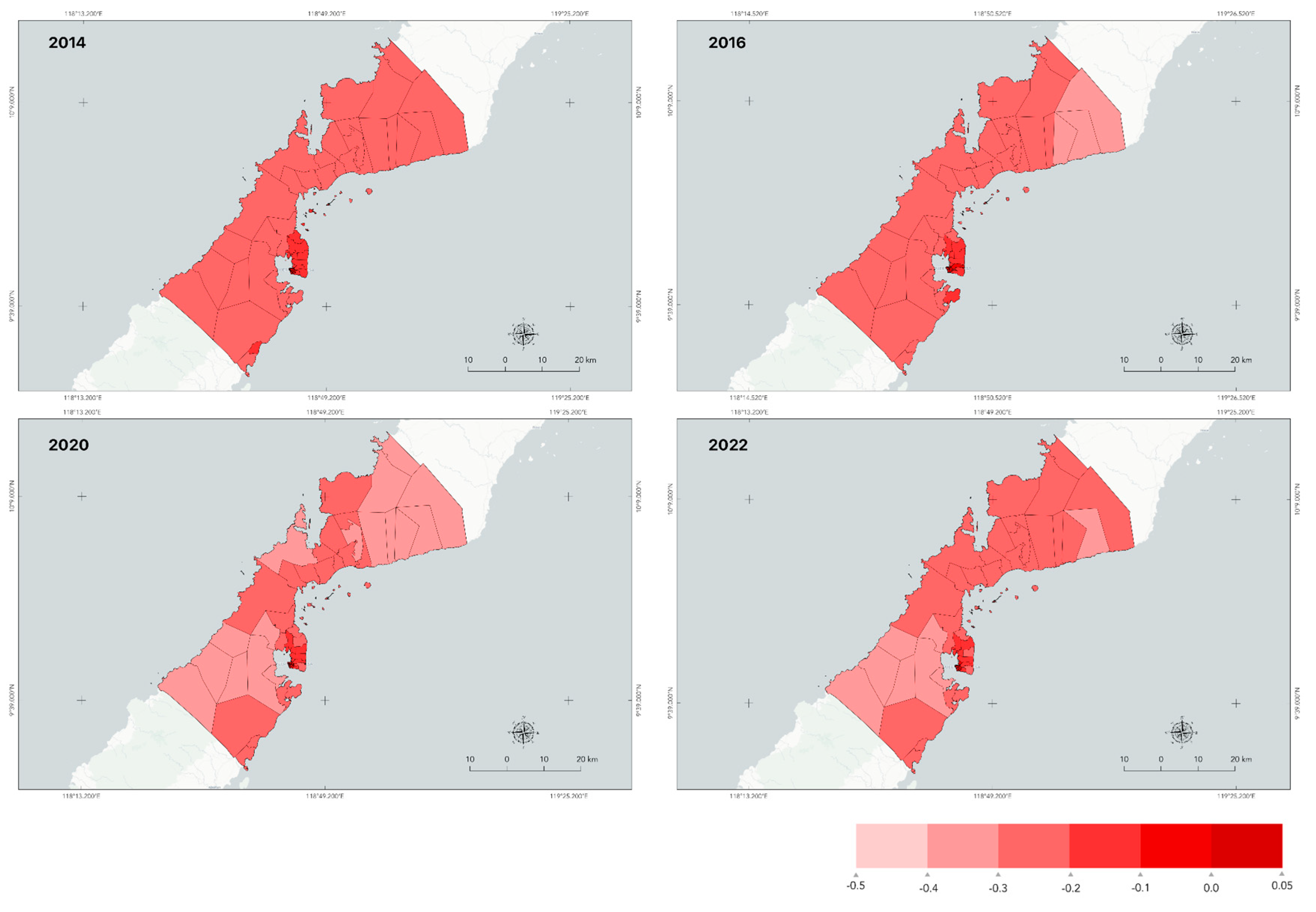
Figure 12 illustrates the identified UHI zones in Puerto Princesa for the years 2014, 2016, 2020, and 2022. Figure 13, on the other hand, summarizes the percentages in the area of the UHI zones in the city. The UHI analysis resulted in an interesting pattern; despite the sudden increase in 2016, data shows a more gradual shift. Moderate UHI zones are identified all across the city, centering around the suburbs and areas with moderate NDVI values, mostly consisting of sparse and mixed vegetation areas. This area has increased to 28.0% in 2022 from only 20.7% in 2014. On the other hand, strong UHI zones, which are centered around the city's main population and commercial centers, decreased from 6.82% in 2014 to only 2.72% in 2022. This suggests a notable shift in the intensity and distribution of the UHI zone in the city over the years. The expansion of moderate UHI zones and the decline of strong UHI zones may indicate an overall intensification of heat across the city, as seen in Figure 10 and Figure 11, leading to a more widespread but less concentrated UHI effect (Shen et al., 2020; Gao et al., 2019)
4. Discussions
4.1. Urban Expansion and Land Cover Change in Puerto Princesa City
Between 2014 and 2022, data suggest that Puerto Princesa City experienced notable population growth and land cover changes, triggering key transformations in its natural and built environment. The LULCC assessment findings showed a steady growth of built-up zones in the city (from 34.4 km² in 2014 to 67.7 km² in 2022), corresponding with an overall trend of rapid population growth in rural barangays and a rise in population density in most urban barangays, suggesting ongoing rural development and urban expansion in these areas (Lu et al., 2023; Gao and O’Neill, 2020).
In the city’s urban zones, the transformation of open spaces into built-up zones is more apparent, particularly in areas along the urban peripheries. This growth suggests economic opportunities are emerging in these peripheral zones, potentially driven by housing demand, lower land costs, and infrastructure development, such as new roads or transport hubs (Angel, 2023; Farah et al., 2019). The LULCC assessment results for rural barangays present a more varied trend, with some experiencing urban expansion, while others remain stagnant, and certain areas even show an increase in forest cover. This is potentially because rural barangays with rapid population growth likely contributed to land conversion, while those experiencing population decline may have seen land abandonment and natural regrowth (Navarro and Pereira, 2015).
Another significant observation in the LULCC assessment is the marked increase in the extent of water bodies in 2022. This change may be attributed to the degradation or loss of coastal and mangrove vegetation due to Typhoon Rai in December 2021, which previously obscured water surfaces. Canopy damage or deforestation in these areas likely made water bodies more detectable in remote sensing analysis, altering their perceived extent (Magallon and Tsuyuki, 2024; Peereman et al., 2021).
4.2. Correlation of NDBI and NDVI with LST
Figure 12 shows the scatter plots of the LST with NDVI (Top plots) and LST with NDBI (Bottom plots) for the years 2014, 2016, 2020, and 2022 (from left to right). The LST was observed to have different plot characteristics for positive and negative NDVI values. Nevertheless, the scatter plot shows a uniform spread of the LST values with NDVI values, suggesting low to no correlation. On the other hand, the scatter plot of LST with NDBI presents an apparent positive correlation, as indicated by the distinctive upward slope of the plot.
The Pearson r correlation coefficients were calculated for each scatter plot in Figure 14 and summarized in Table 5. The NDVI coefficients indicate low to no correlation with LST, as shown by the low correlation values: -0.1537 for 2014, 0.0832 for 2016, -0.1778 for 2020, and -0.0647 for 2022. These results suggest a low negative correlation for 2014, 2020, and 2022, while 2016 shows a very low positive correlation.
NDVI correlation coefficients were also calculated for each land cover type, as shown in Table 6, Table 7, Table 8 and Table 9. Developed and sparse vegetation areas exhibit very low to moderate negative correlations, likely due to the cooling effect of vegetation through evapotranspiration (Zhou, 2023; Ekwe, 2021). Conversely, forest cover shows very low to moderate positive correlations, indicating a competing mechanism that increases LST alongside the cooling effect. One such mechanism is the canopy effect, where heat is trapped and stored in forest canopies, raising the overall LST in the area (Dai, 2023; Shaik, 2023; Zhang, 2022; Richter, 2021). Mixed vegetation covers show a typical low to moderate negative correlation between LST and NDVI for 2014, 2020, and 2022, consistent with the cooling effect of evapotranspiration. However, in 2016, mixed vegetation showed a moderate positive correlation, suggesting a stronger canopy effect compared to evapotranspiration cooling.
The NDBI coefficients indicate moderate to high correlations with LST, with Pearson r values of 0.5284 for 2014, 0.3322 for 2016, 0.4850 for 2020, and 0.3666 for 2022. NDBI correlation coefficients calculated for each land cover type (Table 6, Table 7, Table 8 and Table 9) show a similar trend, except for forest areas. The overall increase in LST with NDBI can be attributed to factors such as a higher Bowen ratio, greater heat retention, and increased heat storage capacity. Built-up areas typically have a lower Bowen ratio due to reduced vegetation cover, diminishing the cooling effect from evapotranspiration. Additionally, urban surfaces — such as bare soil and construction materials — have higher heat retention and storage capacities, increasing net radiation from the land surface and contributing to higher overall LST (Zhao, 2020; Zhao, 2014).
4.3. Trend of LST, NDVI, and NDBI with Population Density
The calculated coefficients and R-squared values for each environmental parameter using the OLS model are presented in Table 10. The corresponding regression lines for each year can be derived by setting the appropriate dummy variables to 1 or 0. For example, setting all dummy variables to zero yields the regression line for the year 2014, while setting the dummy variable to 1 and others to zero gives the regression line for 2016. The scatter plots for NDVI, NDBI, and LST with superimposed regression lines are shown in Figure 13.
The results show a logarithmic decrease in mean NDVI with increasing population density, yielding an R-squared value of 0.800, indicating a very strong correlation. The regression lines reveal an overall temporal trend, with 2016 having the lowest mean NDVI, followed by 2014, 2022, and 2020. This trend is reflected in the dummy variable coefficients: -0.002 for 2016, 0.06 for 2020, and 0.04 for 2022. The small magnitude of the 2016 coefficient suggests NDVI values close to those in 2014. The y-intercept, represented by the coefficient with a value of 0.56, can be interpreted as the NDVI value of bare vegetation when there is no population present. Additionally, the average rate of decrease in NDVI with a tenfold increase in population is -0.04 which is given by the value of the coefficient .
The mean NDBI showed a positive correlation with population density, with an R-squared value of 0.840, again indicating a very strong correlation. The temporal trend observed in the regression lines shows the lowest NDBI in 2020, followed by 2022, 2016, and 2014. The corresponding dummy variable coefficients are -0.002 for 2016, -0.03 for 2020, and -0.02 for 2022, with the low 2016 coefficient indicating NDBI values similar to those in 2014. The y-intercept, -0.39, represents the NDBI value of bare vegetation in the absence of population. The average rate of increase in NDBI with a tenfold increase in population is 0.04.
The model also showed a logarithmic increase in mean LST with population density, with an R-squared value of 0.818, indicating a very strong correlation. The regression lines reveal the lowest LST in 2020, followed by 2014, 2022, and 2016. The corresponding dummy variable coefficients are 1.92 for 2016, -0.12 for 2020, and 1.18 for 2022. The small magnitude of the 2020 coefficient suggests LST values close to those in 2014. The y-intercept, 22.03 °C, represents the LST of bare vegetation with no population influence. Furthermore, the average rate of increase in LST with a tenfold increase in population is 0.77 °C.
4.4. Surface Urban Heat Island (SUHI) Attributions
Urbanization generates small perturbations to the land surface temperature (LST), resulting in LST gradients between urban and rural areas. SUHI, defined as the gradient between urban and rural average land surface temperatures (LST) , can be attributed to different contributions: net solar radiation, anthropogenic heat, air convection, evapotranspiration, and heat storage (Guo, 2024).
To estimate the SUHI, we assumed that rural areas correspond to data points in Figure 15 with a population below 10³ and a mean NDVI of 0.4-0.6, while urban areas have a population above 10³ and a mean NDVI of 0-0.4. The estimated SUHI was calculated as the difference between the average urban and rural land surface temperatures (LST), as shown in Table 11.
The urban and rural average temperatures increased drastically in 2016 due to the strongest El Niño event of the decade (Shiozaki, 2020). Surprisingly, this resulted in a relatively low SUHI of 2.84°C compared to the previous year’s SUHI of 4.77°C, suggesting that rural areas experienced a faster temperature increase than urban areas. One possible explanation is the drying of vegetation, evidenced by the sudden increase in sparse vegetation land cover and a decrease in mixed vegetation. The reduction in the cooling effect normally provided by evapotranspiration may have contributed to the rapid heating of rural areas (Wang, 2023; Yuan, 2023).
By 2020, rural and urban temperatures appeared to have normalized from the 2016 El Niño, as indicated by the gradual recovery of mixed vegetation and a corresponding decrease in sparse vegetation. The lower SUHI value compared to 2014 suggests a greater cooling effect in urban areas, possibly due to increased vegetation within urban spaces or the use of more reflective construction materials (Zhou, 2023; Ekwe, 2021).
In 2022, urban and rural temperatures rose again, with only a minimal reduction in SUHI. This could be attributed to the apparent conversion of mixed and sparse vegetation into developed land cover, potentially as a result of Typhoon Rai damaging coastal or mangrove vegetation (Meneses, 2022).
5. Conclusions
Between 2015 and 2020, a contrasting dynamic played out where population growth was generally greater within the rural context than in urban. Such development indicates continued rural development, growing residential expansion, or increased economic opportunities beyond the urban core of the city. Conversely, urban areas have experienced a fairly steady population density increase, which could result in the development of densely populated communities. Assessing land cover change from 2014 until 2022 shows a notable shift in this period, particularly indicated by the vegetative cover and developed land. Mixed vegetation changed between periods of decline and periods of recovery across the years, but forest cover remained stable. In contrast, developed areas continued to show a steady trend of expansion, reflecting urbanization and infrastructure development. The rural-urban contrast is further highlighted by the NDVI and NDBI values. Because of their dense development, urban areas had lower NDVI values, whereas rural areas continued to have higher and more stable vegetation indices. On the other hand, NDBI values were higher in the built-up areas of urban centers, though some areas experienced a decline, indicating either a slowdown in expansion or a rise in urban greening initiatives.
The LST analysis shows an overall increasing trend, with urban areas consistently recording higher temperatures than rural regions. This aligns with the urban heat island UHI effect, where built-up environments retain more heat compared to vegetated landscapes. Over time, strong UHI zones have decreased, while moderate UHI zones have expanded, indicating a more dispersed but less intense heat concentration across the city. The analysis reveals a distinct correlation between LST and land cover characteristics, particularly through the NDBI and NDVI. While NDVI showed a low correlation with LST, NDBI exhibited a moderate to high positive correlation, indicating that built-up areas contribute significantly to increased surface temperatures, possibly due to factors such as heat retention and reduced evapotranspiration. The regression analysis further highlights the strong relationship between population density and environmental parameters, with increasing urbanization leading to higher LST and NDBI, and decreasing NDVI.
The findings of this study suggest that the city is undergoing significant demographic and environmental transformations driven by urban expansion, land use changes, and climate-related factors. While rural areas are experiencing rapid growth, urban centers continue to densify, impacting vegetation cover and temperature dynamics, highlighting the need for a balanced strategy for sustainability and urban resilience. It is recommended that future research be taken to examine deeper specific attributing factors to increasing temperatures, driving factors of land cover change, and effectiveness of current sustainability mechanisms in the city.
References
- Abbas, S.; Nichol, J.E.; Fischer, G.A.; Wong, M.S.; Irteza, S.M. 2019. Impact assessment of a super-typhoon on Hong Kong’s secondary vegetation and recommendations for restoration of resilience in the forest succession. Agricultural and Forest Meteorology, 280: 107784. [CrossRef]
- Ahmad, F.; Uddin, M.M.; Goparaju, L. 2018. An evaluation of vegetation health and the socioeconomic dimension of the vulnerability of Jharkhand state of India in climate change scenarios and their likely impact: a geospatial approach. Environmental & Socio-economic Studies, 6: 39–47. [CrossRef]
- Alademomi, A.S.; Okolie, C.J.; Daramola, O.E.; Akinnusi, S.A.; Adediran, E.; Olanrewaju, H.O.; Alabi, A.O.; Salami, T.J.; Odumosu, J. 2022. The interrelationship between LST, NDVI, NDBI, and land cover change in a section of Lagos metropolis, Nigeria. Applied Geomatics, 14: 299–314. [CrossRef]
- Angel, S. 2023. Urban expansion: theory, evidence, and practice. Buildings and Cities, 4: 124–138. [CrossRef]
- Choudhury, D.; Das, K.; Das, A. 2018. Assessment of land use land cover changes and its impact on variations of land surface temperature in Asansol-Durgapur Development Region. The Egyptian Journal of Remote Sensing and Space Science, 22: 203–218. [CrossRef]
- Dai, J. ping, Qin, J. zheng, Zhou, T.; Qin, X. jian, Zhu, K.; Peng, J. song. 2023. Study on the influence of urban tree canopy on thermal environment in Luoping County. Scientific Reports 13. [CrossRef]
- Dong, W.; Liu, Z.; Zhang, L.; Tang, Q.; Liao, H.; Li, X. 2014. Assessing heat health risk for sustainability in Beijing’s urban heat island. Sustainability, 6: 7334–7357. [CrossRef]
- Ekwe, M.C.; Adamu, F.; Gana, J.; Nwafor, G.C.; Usman, R.; Nom, J.; Onu, O.D.; Adedeji, O.I.; Halilu, S.A.; Aderoju, O.M. 2021. The effect of green spaces on the urban thermal environment during a hot-dry season: a case study of Port Harcourt, Nigeria. Environment, Development and Sustainability 23. 2021. [CrossRef]
- Farah, N.; Khan, Maan, Shahbaz, B.; Cheema, M.J.M. 2019. Driving factors of agricultural land conversion at rural-urban interface in Punjab, Pakistan. Journal of Agricultural Research, 57: 55–62. https://apply.jar.punjab.gov.pk/upload/1561448694_135_9._1354.pdf.
- Gang, C.; Pan, S.; Tian, H.; Wang, Z.; Xu, R.; Bian, Z.; Pan, N.; Yao, Y.; Shi, H. 2020. Satellite observations of forest resilience to hurricanes along the northern Gulf of Mexico. Forest Ecology and Management, 472, 118243. [CrossRef]
- Gao, J.; O’Neill, B.C. 2020. Mapping global urban land for the 21st century with data-driven simulations and Shared Socioeconomic Pathways. Nature Communications, 11. [CrossRef]
- Gao, Z.; Hou, Y.; Chen, W. 2019. Enhanced sensitivity of the urban heat island effect to summer temperatures induced by urban expansion. Environmental Research Letters, 14: 094005. [CrossRef]
- Gill, J.C.; Malamud, B.D. 2017. Anthropogenic processes, natural hazards, and interactions in a multi-hazard framework. Earth-Science Reviews, 166, 246–269. [CrossRef]
- Guo, F.; Hertel, D.; Schlink, U.; Hu, D.; Qian, J.; Wu, W. 2024. Remote Sensing-Based Attribution of Urban Heat Islands to the Drivers of Heat. IEEE Transactions on Geoscience and Remote Sensing, 62. [CrossRef]
- Hugo, G. 2019. Patterns and Trends of urbanization and urban growth in Asia. In Springer eBooks (pp. 13–45). [CrossRef]
- Landsberg, H.E. 1981. The urban climate. In Google Books: Vol. Volume 28. Academic Press. https://books.google.com.ph/books/about/The_Urban_Climate.html?id=zkKHiEXZGBIC&redir_esc=y.
- Lu, H.; Shang, Z.; Ruan, Y.; Jiang, L. 2023. Study on urban expansion and population density changes based on the inverse S-Shaped function. Sustainability, 15: 10464. [CrossRef]
- Magallon, B.J.P.; Tsuyuki, S. 2024. Typhoon-Induced forest damage mapping in the Philippines using Landsat and PlanetScope images. Land, 13: 1031. [CrossRef]
- Meneses, S.F.; Blanco, A.C. 2022. Rapid mapping and assessment of damages due to Typhoon Rai were conducted using Sentinel-1 synthetic aperture radar data. International Archives of the Photogrammetry, Remote Sensing and Spatial Information Sciences - ISPRS Archives, 43(B3-2022). [CrossRef]
- Mondo, J.M.; Chuma, G.B.; Muke, M.B.; Fadhili, B.B.; Kihye, J.B.; Matiti, H.M.; Sibomana, C.I.; Kazamwali, L.M.; Kajunju, N.B.; Mushagalusa, G.N.; Karume, K.; Mambo, H.; Ayagirwe, R.B.; Balezi, A.Z. 2024. Utilization of non-timber forest products as alternative sources of food and income in the highland regions of the Kahuzi-Biega National Park, eastern Democratic Republic of Congo. Trees Forests and People, 16, 100547. [CrossRef]
- Navarro, L.M.; Pereira, H.M. 2015. Rewilding abandoned landscapes in Europe. In Springer eBooks (pp. 3–23). [CrossRef]
- Nguyen, T.; Lin, T.; Chan, H. 2019. The Environmental Effects of Urban Development in Hanoi, Vietnam from Satellite and Meteorological Observations from 1999–2016. Sustainability, 11: 1768. [CrossRef]
- Patra, S.; Sahoo, S.; Mishra, P.; Mahapatra, S.C. 2018. Impacts of urbanization on land use /cover changes and its probable implications on local climate and groundwater level. Journal of Urban Management, 7: 70–84. [CrossRef]
- Peereman, J.; Hogan, J.A.; Lin, T. 2021. Disturbance frequency, intensity and forest structure modulate cyclone-induced changes in mangrove forest canopy cover. Global Ecology and Biogeography, 31: 37–50. [CrossRef]
- Richter, R.; Hutengs, C.; Wirth, C.; Bannehr, L.; Vohland, M. 2021. Detecting tree species effects on forest canopy temperatures with thermal remote sensing: The role of spatial resolution. Remote Sensing, 13. [CrossRef]
- Santillan, J.R.; Heipke, C. 2024. Assessing patterns and trends in urbanization and land use efficiency across the Philippines: a comprehensive analysis using global Earth observation data and SDG 11.3.1 indicators. PFG – Journal of Photogrammetry Remote Sensing and Geoinformation Science, 92: 569–592. [CrossRef]
- Shaik, R.U.; Jallu, S.B.; Doctor, K. 2023. Unveiling Temperature Patterns in Tree Canopies across Diverse Heights and Types. Remote Sensing, 15. [CrossRef]
- Shen, Z.; Shi, J.; Tan, J.; Yang, H. 2020. The migration of the Warming Center and urban Heat island effect in Shanghai during urbanization. Frontiers in Earth Science, 8. [CrossRef]
- Shiozaki, M.; Enomoto, T. 2020. Comparison of the 2015/16 El Niño with the two previous strongest events. Scientific Online Letters on the Atmosphere, 16. [CrossRef]
- Soe, K.T.; Yeo-Chang, Y. 2019. Livelihood Dependency on Non-Timber Forest products: Implications for REDD+. Forests, 10: 427. [CrossRef]
- USGS. 2019. Landsat 8 Data Users Handbook. https://www.usgs.gov/landsat-missions/landsat-8-data-users-handbook.
- Wang, Y.; Shi, H.; Jiang, Y.; Wu, Y.; Gao, Y.; Ding, C. 2023. Spatiotemporal Variation of Drought Characteristics and Its Influencing Factors in Loess Plateau Based on TVDI. Nongye Jixie Xuebao/Transactions of the Chinese Society for Agricultural Machinery, 54. [CrossRef]
- Yuan, Y.; Ye, X.; Liu, T.; Li, X. 2023. Drought monitoring based on temperature vegetation dryness index and its relationship with anthropogenic pressure in a subtropical humid watershed in China. Ecological Indicators, 154. [CrossRef]
- Zhang, X.; Chen, G.; Cai, L.; Jiao, H.; Hua, J.; Luo, X.; Wei, X. 2021. Impact assessments of typhoon Lekima on forest damages in subtropical China using machine learning methods and LanDsat 8 OLI imagery. Sustainability, 13: 4893. [CrossRef]
- Zhang, Z.; Li, X.; Liu, H. 2022. Biophysical feedback of forest canopy height on land surface temperature over contiguous United States. Environmental Research Letters, 17. [CrossRef]
- Zhao, L.; Lee, X.; Smith, R.B.; Oleson, K. 2014. Strong contributions of local background climate to urban heat islands. Nature, 511. [CrossRef]
- Zhao, J.; Zhao, X.; Liang, S.; Zhou, T.; Du, X.; Xu, P.; Wu, D. 2020. Assessing the thermal contributions of urban land cover types. Landscape and Urban Planning, 204. [CrossRef]
- Zhou, S.; Zheng, H.; Liu, X.; Gao, Q.; Xie, J. 2023. Identifying the Effects of Vegetation on Urban Surface Temperatures Based on Urban–Rural Local Climate Zones in a Subtropical Metropolis. Remote Sensing, 15. [CrossRef]
Figure 4.
Change in population density per km² in barangays of Puerto Princesa City from 2015 to 2020 arranged from rural (left) to urban (right) barangays (Data Source: Philippine Statistics Authority).
Figure 4.
Change in population density per km² in barangays of Puerto Princesa City from 2015 to 2020 arranged from rural (left) to urban (right) barangays (Data Source: Philippine Statistics Authority).
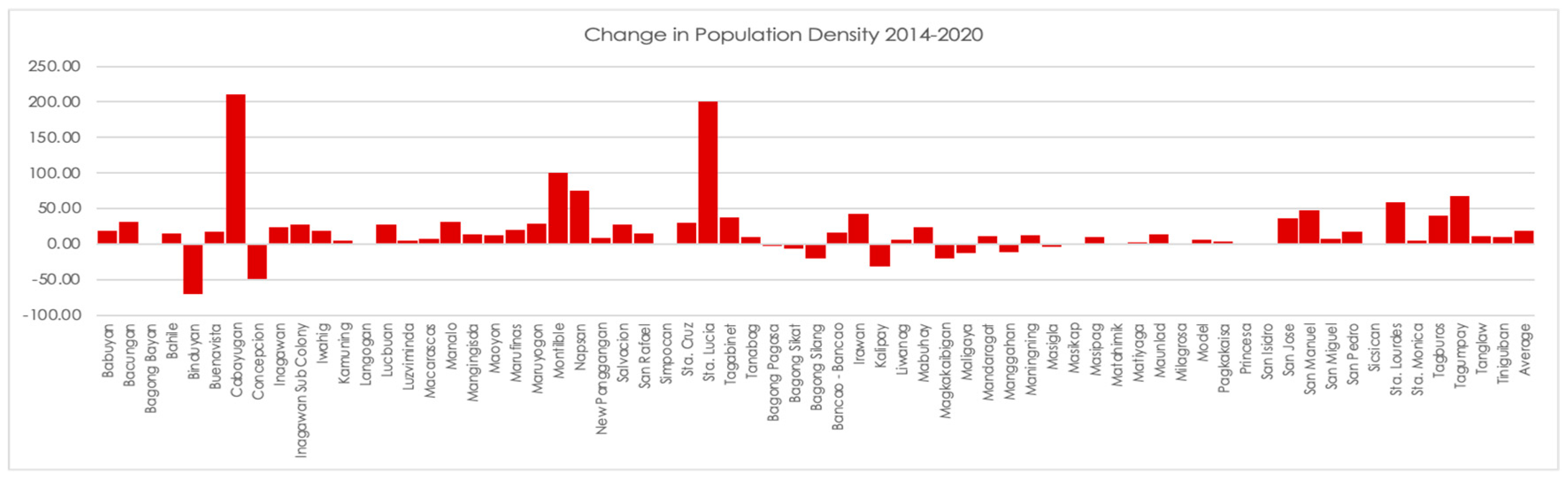
Figure 5.
Generated land cover maps of Puerto Princesa City for the years 2014, 2016, 2020, and 2022.
Figure 5.
Generated land cover maps of Puerto Princesa City for the years 2014, 2016, 2020, and 2022.
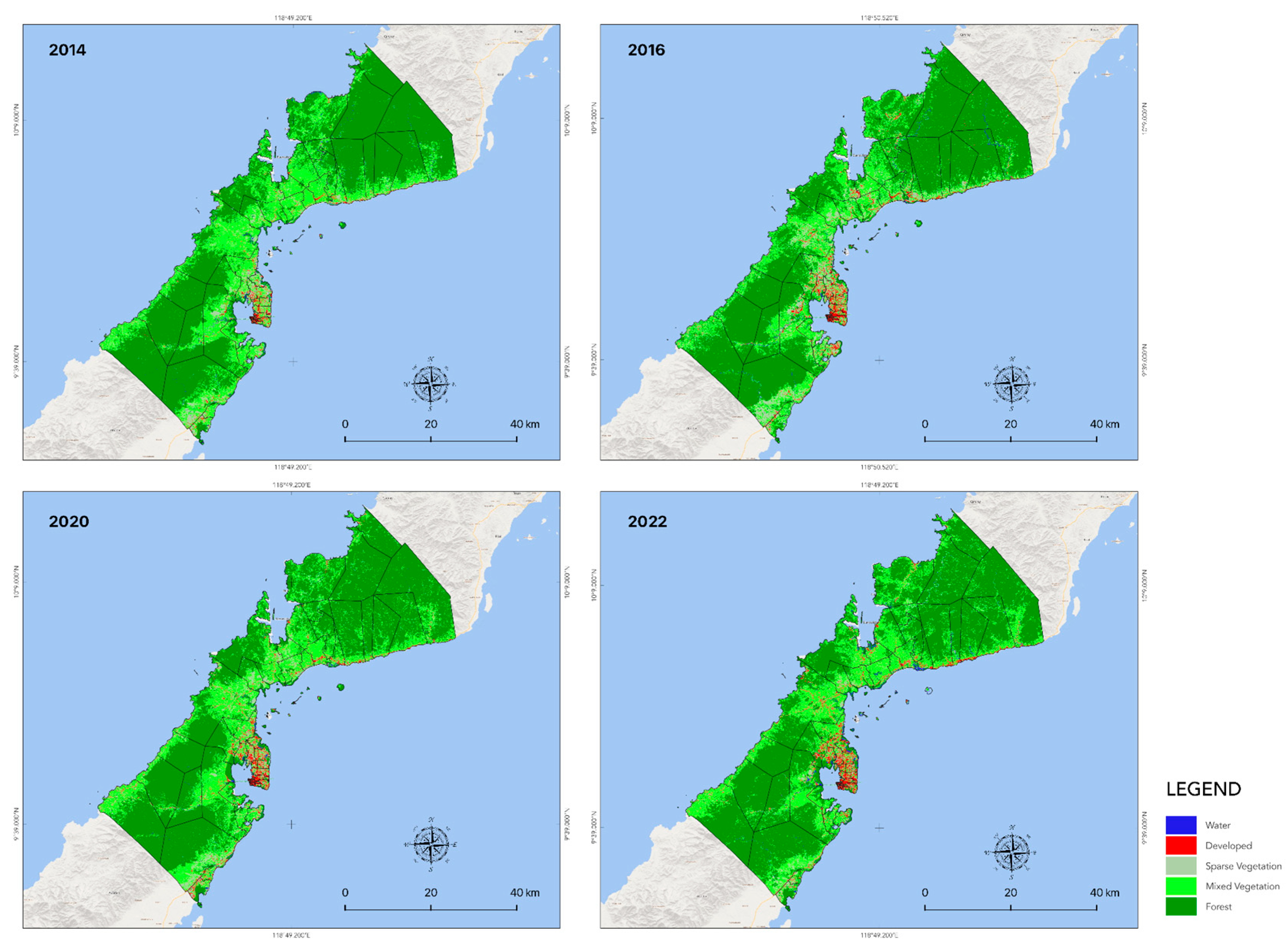
Figure 10.
Maps representing mean LST values across the barangays of Puerto Princesa City from 2014 to 2022.
Figure 10.
Maps representing mean LST values across the barangays of Puerto Princesa City from 2014 to 2022.
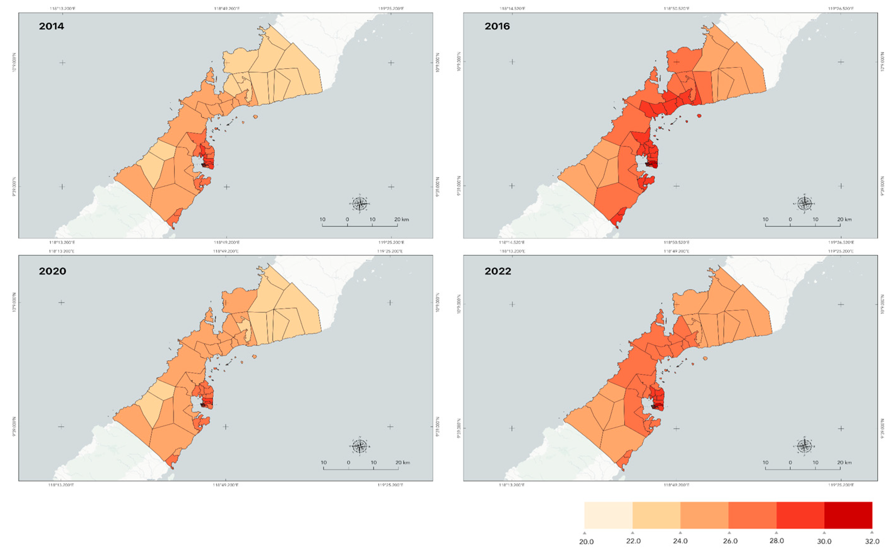
Figure 11.
Mean LST values across the barangays of Puerto Princesa City arranged from highest (left) to lowest (right) density.
Figure 11.
Mean LST values across the barangays of Puerto Princesa City arranged from highest (left) to lowest (right) density.
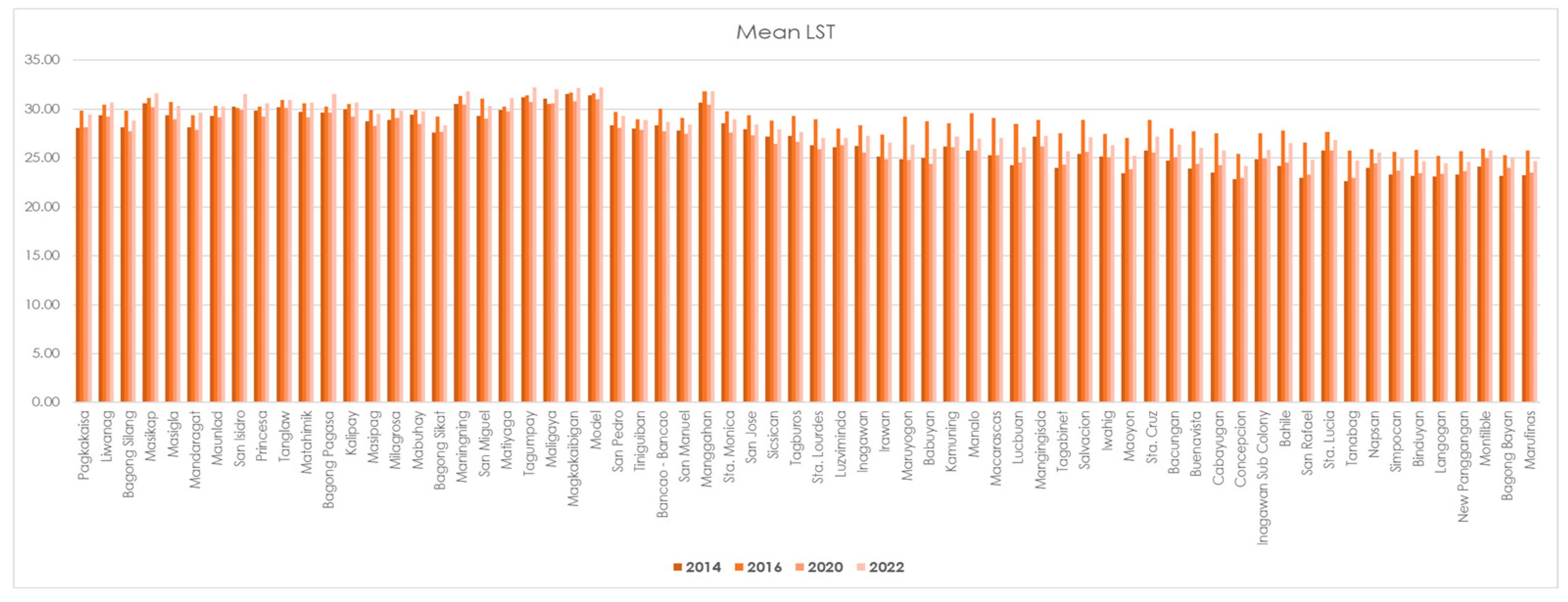
Figure 12.
Maps of UHI zones in Puerto Princesa in the varying years of 2014, 2016, 2020, and 2022.
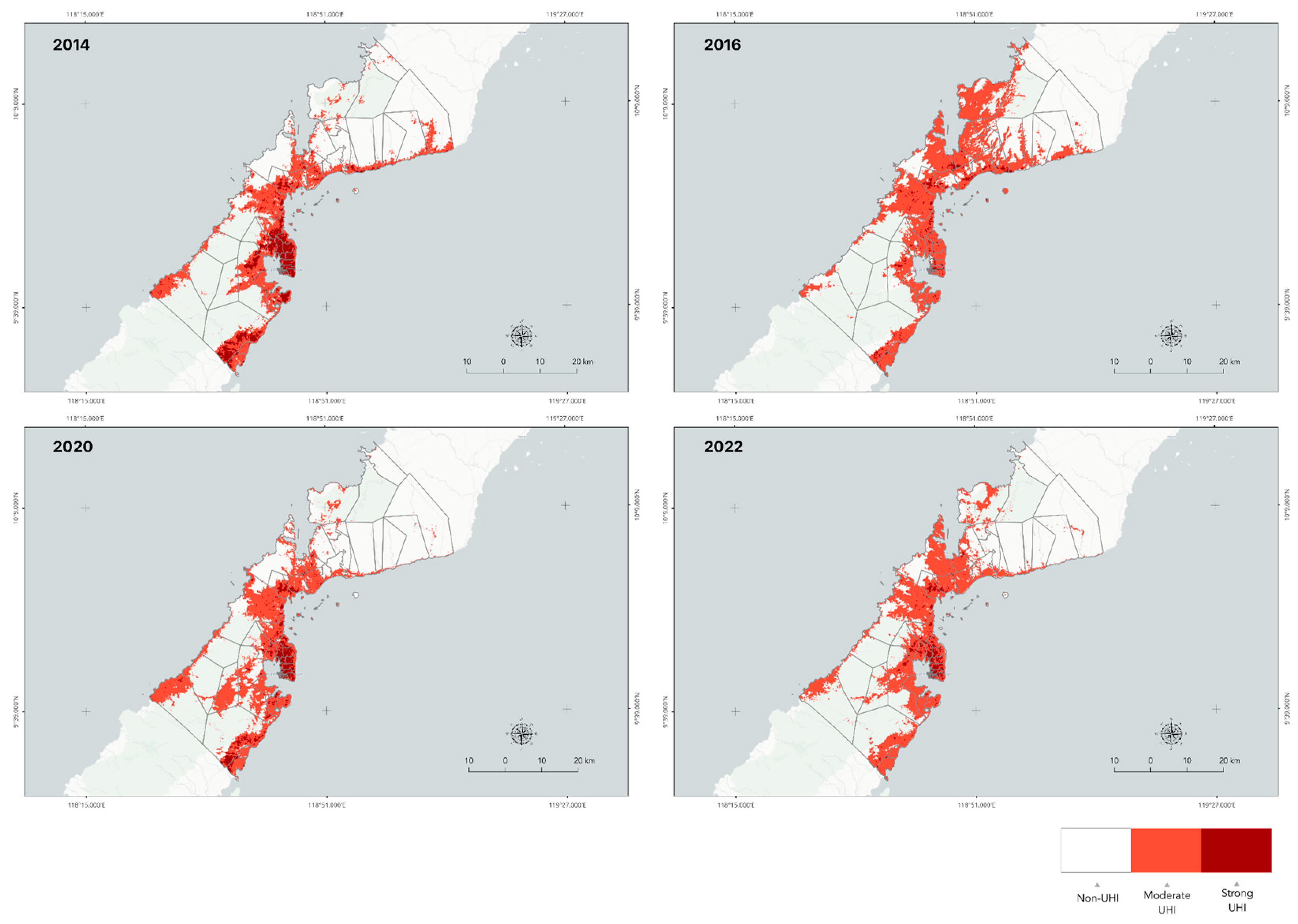
Figure 13.
Graph showing the distribution of UHI zones in Puerto Princesa in the varying years of 2014, 2016, 2020, and 2022.
Figure 13.
Graph showing the distribution of UHI zones in Puerto Princesa in the varying years of 2014, 2016, 2020, and 2022.
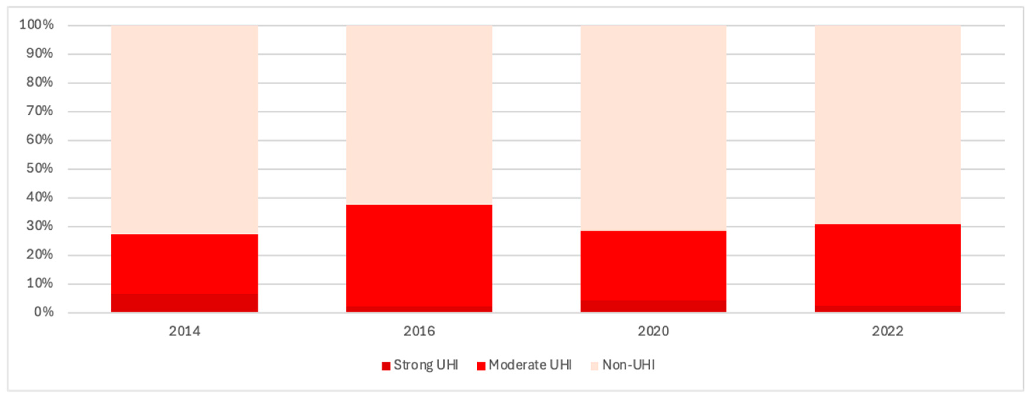
Figure 14.
Scatter diagrams of Land Surface Temperature (LST) with Normalized Difference Built-up Index (NDBI) and Normalized Difference Vegetation Index (NDVI) for the years 2014, 2016, 2020, and 2022.
Figure 14.
Scatter diagrams of Land Surface Temperature (LST) with Normalized Difference Built-up Index (NDBI) and Normalized Difference Vegetation Index (NDVI) for the years 2014, 2016, 2020, and 2022.
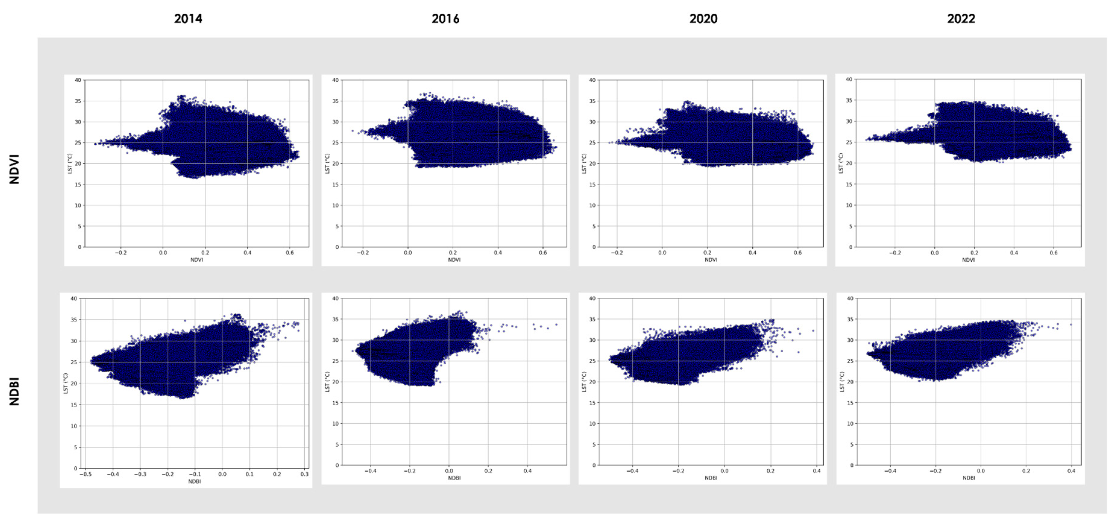
Figure 15.
Scatter plots of the environmental parameters (LST, NDVI, and NDBI) with population density along the regression lines for each year obtained from the OLS model.
Figure 15.
Scatter plots of the environmental parameters (LST, NDVI, and NDBI) with population density along the regression lines for each year obtained from the OLS model.
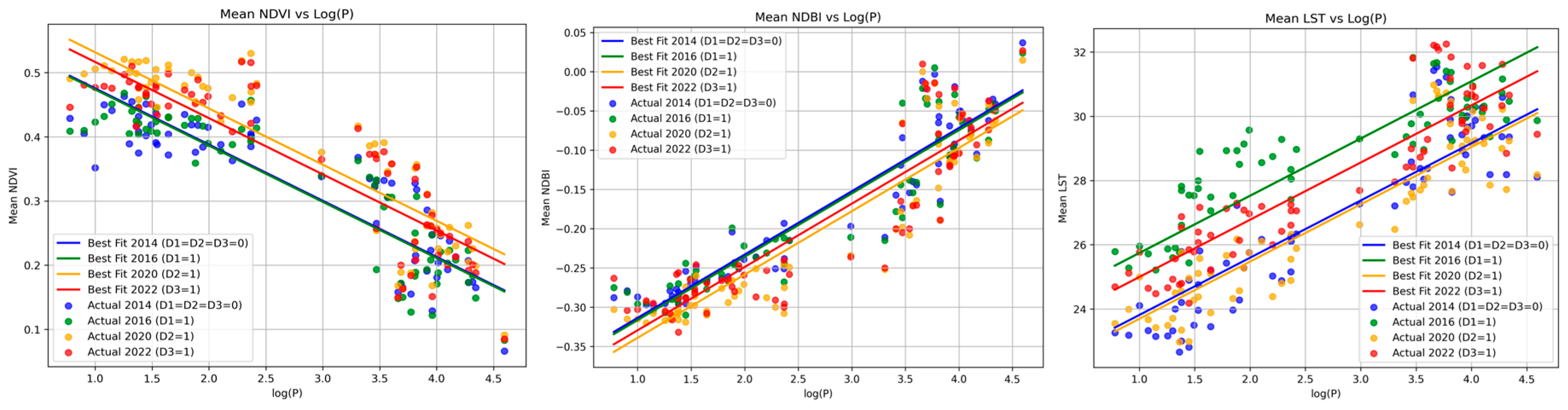

Table 1.
Landsat images utilized for NDBI, NDVI, and LST calculations.
| Year | Landsat Series | Date of Acquisition | Sensor | Row | Path |
|---|---|---|---|---|---|
| 2014 | Landsat 8 | 03/02/2014 | OLI/TIRS | 053 | 117 |
| 2016 | Landsat 8 | 01/19/2016 | OLI/TIRS | 053 | 117 |
| 2020 | Landsat 8 | 08/25/2020 | OLI/TIRS | 053 | 117 |
| 2022 | Landsat 8 | 06/12/2022 | OLI/TIRS | 053 | 117 |
Table 2.
Transition matrix of the land cover change from year 2014 to year 2016.
| Land Cover class | 2016 | ||||||
| Water | Developed | Sparse vegetation | Forest | Mixed Vegetation | 2014 TOTAL |
||
| 2014 | Water | 8.1 | 0.3 | 1.4 | 7.7 | 4.2 | 21.8 |
| Developed | 0.9 | 22.5 | 1.7 | 3.3 | 5.8 | 34.4 | |
| Sparse vegetation | 0.5 | 13.0 | 31.3 | 10.9 | 26.1 | 81.8 | |
| Forest | 3.4 | 4.2 | 7.6 | 1215.5 | 134.8 | 1365.5 | |
| Mixed Vegetation | 1.8 | 19.5 | 71.8 | 204.2 | 390.8 | 688.1 | |
| Total | 14.8 | 59.6 | 113.8 | 1441.6 | 561.8 | 2191.5 | |
Table 3.
Transition matrix of the land cover change from year 2016 to year 2017.
| Land Cover class | 2020 | ||||||
| Water | Developed | Sparse vegetation | Forest | Mixed Vegetation | 2016 TOTAL |
||
| 2016 | Water | 8.1 | 1.0 | 0.4 | 3.5 | 2.3 | 15.2 |
| Developed | 0.8 | 30.9 | 8.9 | 5.8 | 13.2 | 59.7 | |
| Sparse vegetation | 2.4 | 7.3 | 27.7 | 11.7 | 65.1 | 114.3 | |
| Forest | 5.4 | 4.8 | 12.9 | 1199.3 | 219.5 | 1442.0 | |
| Mixed Vegetation | 1.9 | 17.1 | 32.8 | 154.9 | 355.1 | 561.7 | |
| Total | 18.5 | 61.1 | 82.8 | 1375.2 | 655.1 | 2192.8 | |
Table 4.
Transition matrix of the land cover change from year 2016 to year 2020.
| Land Cover class | 2022 | ||||||
| Water | Developed | Sparse vegetation | Forest | Mixed Vegetation | 2020 TOTAL |
||
| 2020 | Water | 11.0 | 0.1 | 0.2 | 5.1 | 2.0 | 18.4 |
| Developed | 2.6 | 35.5 | 5.8 | 3.6 | 13.7 | 61.2 | |
| Sparse vegetation | 1.3 | 10.3 | 15.5 | 12.4 | 43.3 | 82.8 | |
| Forest | 13.1 | 4.3 | 6.9 | 1196.2 | 153.4 | 1373.9 | |
| Mixed Vegetation | 4.1 | 17.4 | 11.7 | 188.2 | 433.8 | 655.1 | |
| Total | 32.1 | 67.7 | 40.0 | 1405.5 | 646.2 | 2191.5 | |
Table 5.
Pearson correlation coefficients of Land Surface Temperature (LST) with Normalized Difference Built-up Index (NDBI) and Normalized Difference Vegetation Index (NDVI).
Table 5.
Pearson correlation coefficients of Land Surface Temperature (LST) with Normalized Difference Built-up Index (NDBI) and Normalized Difference Vegetation Index (NDVI).
| LST | NDBI Pearson r (p<0.0001) | NDVI Pearson r (p<0.0001) |
| 2014 | 0.5284 | -0.1537 |
| 2016 | 0.3322 | 0.0832 |
| 2020 | 0.4850 | -0.1778 |
| 2022 | 0.3666 | -0.0647 |
Table 6.
Pearson correlation coefficients of Land Surface Temperature (LST) with Normalized Difference Built-up Index (NDBI) and Normalized Difference Vegetation Index (NDVI) for each land cover class in 2014.
Table 6.
Pearson correlation coefficients of Land Surface Temperature (LST) with Normalized Difference Built-up Index (NDBI) and Normalized Difference Vegetation Index (NDVI) for each land cover class in 2014.
| Land Cover | r (LST vs NDVI) | p-value (NDVI) | r (LST vs NDBI) | p-value (NDBI) |
| Water | -0.14 | p<0.0001 | 0.13 | p<0.0001 |
| Developed | -0.23 | p<0.0001 | 0.68 | p<0.0001 |
| Sparse vegetation | -0.20 | p<0.0001 | 0.68 | p<0.0001 |
| Forest | 0.14 | p<0.0001 | 0.08 | p<0.0001 |
| Mixed Vegetation | -0.20 | p<0.0001 | 0.53 | p<0.0001 |
Table 7.
Pearson correlation coefficients of Land Surface Temperature (LST) with Normalized Difference Built-up Index (NDBI) and Normalized Difference Vegetation Index (NDVI) for each land cover class in 2016.
Table 7.
Pearson correlation coefficients of Land Surface Temperature (LST) with Normalized Difference Built-up Index (NDBI) and Normalized Difference Vegetation Index (NDVI) for each land cover class in 2016.
| Land Cover | r (LST vs NDVI) | p-value (NDVI) | r (LST vs NDBI) | p-value (NDBI) |
| Water | -0.24 | p<0.0001 | 0.27 | p<0.0001 |
| Developed | -0.04 | p<0.0001 | 0.60 | p<0.0001 |
| Sparse vegetation | 0.02 | p<0.0001 | 0.52 | p<0.0001 |
| Forest | 0.31 | p<0.0001 | -0.03 | p<0.0001 |
| Mixed Vegetation | 0.24 | p<0.0001 | 0.23 | p<0.0001 |
Table 8.
Pearson correlation coefficients of Land Surface Temperature (LST) with Normalized Difference Built-up Index (NDBI) and Normalized Difference Vegetation Index (NDVI) for each land cover class in 2020.
Table 8.
Pearson correlation coefficients of Land Surface Temperature (LST) with Normalized Difference Built-up Index (NDBI) and Normalized Difference Vegetation Index (NDVI) for each land cover class in 2020.
| Land Cover | r (LST vs NDVI) | p-value (NDVI) | r (LST vs NDBI) | p-value (NDBI) |
| Water | -0.26 | p<0.0001 | 0.25 | p<0.0001 |
| Developed | -0.35 | p<0.0001 | 0.63 | p<0.0001 |
| Sparse vegetation | -0.24 | p<0.0001 | 0.58 | p<0.0001 |
| Forest | 0.12 | p<0.0001 | 0.06 | p<0.0001 |
| Mixed Vegetation | -0.19 | p<0.0001 | 0.44 | p<0.0001 |
Table 9.
Pearson correlation coefficients of Land Surface Temperature (LST) with Normalized Difference Built-up Index (NDBI) and Normalized Difference Vegetation Index (NDVI) for each land cover class in 2022.
Table 9.
Pearson correlation coefficients of Land Surface Temperature (LST) with Normalized Difference Built-up Index (NDBI) and Normalized Difference Vegetation Index (NDVI) for each land cover class in 2022.
| Land Cover | r (LST vs NDVI) | p-value (NDVI) | r (LST vs NDBI) | p-value (NDBI) |
| Water | 0.01 | <0.05 | 0.13 | <0.0001 |
| Developed | -0.27 | <0.0001 | 0.61 | <0.0001 |
| Sparse vegetation | -0.12 | <0.0001 | 0.53 | <0.0001 |
| Forest | 0.20 | <0.0001 | -0.03 | <0.0001 |
| Mixed Vegetation | -0.33 | <0.0001 | 0.45 | <0.0001 |
Table 10.
Calculated coefficients and R-squared of the Ordinary Least Square (OLS) regression model for the environmental parameters LST, NDVI, and NDBI.
Table 10.
Calculated coefficients and R-squared of the Ordinary Least Square (OLS) regression model for the environmental parameters LST, NDVI, and NDBI.
| Y | R-squared | |||||
| LST | 22.03 | 0.77 | 1.92 | -0.12 | 1.18 | 0.818 |
| NDVI | 0.56 | -0.04 | -0.002 | 0.06 | 0.04 | 0.800 |
| NDBI | -0.39 | 0.04 | -0.002 | -0.03 | -0.02 | 0.840 |
Table 11.
Calculated SUHI from the average urban and rural LST.
| 2014 | 2016 | 2020 | 2022 | |
| LSTrural | 24.53°C | 27.42°C | 24.67°C | 25.99°C |
| LSTurban | 29.30°C | 30.27°C | 28.92°C | 30.20°C |
| SUHI() | 4.77°C | 2.84°C | 4.26°C | 4.21°C |
Disclaimer/Publisher’s Note: The statements, opinions and data contained in all publications are solely those of the individual author(s) and contributor(s) and not of MDPI and/or the editor(s). MDPI and/or the editor(s) disclaim responsibility for any injury to people or property resulting from any ideas, methods, instructions or products referred to in the content. |
© 2025 by the authors. Licensee MDPI, Basel, Switzerland. This article is an open access article distributed under the terms and conditions of the Creative Commons Attribution (CC BY) license (http://creativecommons.org/licenses/by/4.0/).
Copyright: This open access article is published under a Creative Commons CC BY 4.0 license, which permit the free download, distribution, and reuse, provided that the author and preprint are cited in any reuse.


