
Submitted:
24 April 2025
Posted:
25 April 2025
You are already at the latest version
Abstract
In this paper, we develop a new family of distributions supported on a bounded interval with a probability density function that is constructed from two elliptical arcs. The distribution can take on a variety of shapes and has three basic parameters- minimum, maximum, and mode. We give general expression for the density and distribution function of the new distribution. Properties of this distribution are studied and parameter estimation is discussed. Monte Carlo simulation results show the performance of our estimators under many sets of situations. Further, we show the advantages of our distribution over the commonly used triangular distribution in approximating beta distributions.
Keywords:
triangular distribution
; maximum likelihood
; bi-elliptic distribution
1. Introduction
The topic of continuous distributions on a bounded interval is an important aspect of statistical theory and applications. In recent years, many researchers have focused their attention on developing such distributions and their applications (Kotz and Dorp, 2004; García et al., 2011; Condino and Domma, 2017). Beta distribution is one of the most popular bounded distributions and is useful in many areas of application because it provides a rich family of distributional shapes over some finite interval (Goel and Strebel, 1984; McDonald and Xu, 1995; Gupta and Nadarajah, 2004). Researchers developed suitable substitutes of the beta distribution over the years. For instance, the triangular distribution has been investigated by D. Johnson (1997) as a proxy for the beta distribution in risk analysis. Many extensions have been proposed over the years. The trapezoidal distribution was constructed by adding an additional horizontal line segment in the middle and thus provides a more flexible distribution. It was used to model the duration and the form of a phenomenon which maybe represented by three stages: a growth-stage, a stable stage, and a decline stage in Dorp and Kotz (2003). Dorp and Kotz (2002) developed a new family of distributions named the two-sided power distribution and discussed its parameter estimation. Karlis and Xekalaki (2008) introduced another class of distributions called the polygonal distributions constructed from finite mixtures of the triangular distributions. Vander Wielen and Vander Wielen (2015) proposed the general segmented distributions constructed from a finite number of line segments.
In this paper, a new class of distributions is developed using two elliptical arcs connecting together over a bounded interval. We term this distribution the bi-elliptic distribution. Similar to the triangular distribution, it is a unimodal distribution with three parameters: the minimal value a, the maximal value b, and the mode m. The proposed distribution has several advantages in probability modeling. First, it is differentiable at all points over its support. Unlike the triangular distribution and other similar truncated distributions, the density function of the bi-elliptic distribution is differential everywhere in its domain, making it a better choice analytically. Second, the proposed distribution has a flatter shape around its mode, making it a better modeling choice for certain physical and social science phenomena of interest. For instance, small businesses usually experience slow growth and decline when they reach the stage of maturity (Scott and Bruce,1987). Third, the three parameters in the distribution provide large flexibility in modeling. For instance, the distribution can be negatively skewed, positively skewed, and symmetric. Finally, similar to the triangular distribution, the bi-elliptic distribution is based on a knowledge of the minimum, maximum, and the most common modal value, enabling it to work when data are limited. For instance, it can be used in quantitatively analyzing the uncertainty of three-point-estimate problems (Mulligan, 2016).
The paper is organized as follows. Section 2 presents the bi-elliptic distribution and its basic properties. In Section 3, the maximum likelihood estimation (MLE) procedure for bi-elliptic distributions is discussed. Section 4 presents a wide range of Monte-Carlo simulation results for parameter estimation. Section 5 compares the triangular distribution and the proposed bi-elliptic distribution in fitting data drawn from a range of beta distributions. Finally, we provide some concluding remarks in Section 6.
2. The Bi-Elliptic Distribution
Let X be a random variable with a probability density function given by
where , , and . The random variable X is said to have a bi-elliptic distribution, , . Here a is the lower limit, b is the the upper limit, and m is the mode. In addition, bi-elliptic distributions also include two extreme cases when or :
We call the bi-elliptic distribution with and the standard bi-elliptic distribution. For any bi-elliptic distribution , the following property holds:
Figure 1 provides the density plots of examples of symmetric, positively and negatively skewed distributions for different choices of m values. As we can see, the distribution is right-skewed if ; it is left-skewed if ; the distribution is symmetric if .
The cumulative distribution function of an distribution can be derived from equation (1) and is given below
Figure 2 provides plots of the distribution function for examples of symmetric, positively and negatively skewed distributions for different choices of m values.
For any bi-elliptic distribution, m is the mode and the -quantile with .
The median of a bi-elliptic distribution is the unique real value x for which . There is no general closed-form expression for the median. However, for symmetric cases when , the median is the mode m.
The first three moments and the variance of can be obtained from the density function (1) and simplified as follows:
Note that the skewness of X can be expressed in term of the first three moments of X:
3. Parameter Estimation
3.1. Maximum Likelihood Estimation
For a random sample of size n from an distribution, let the order statistics be . Using expression (1), the likelihood function for can be obtained as follows:
where
and s is implicitly defined by
We have the following partial derivatives:
3.2. One-Parameter Maximum Likelihood Estimation
The one-parameter case is of special interest because in some applications, there exist natural lower and upper bounds for random variables of interests. For instance, in hydrology, the reservoir yield and storage distribution has an natural upper bound being its capacity and a lower bound being zero (Fletcher and Ponnambalam, 1996).
When and are fixed and known, taking the partial derivative of the log-likelihood function with respect to m yields equation (18), whose critical point(s) do not have an explicit form. The one-parameter maximum likelihood estimation is an optimization problem below:
or, equivalently,
where and are given by equations (12) and (14), respectively, with a and b being replaced by and . This optimization problem can be solved using numerical methods. For instance, we use Brent’s algorithm for the numerical computations which combines linear interpolation and inverse quadratic interpolation with bisection for one-dimensional optimization problems. Interested readers may refer to Brent (1971) for more details.
3.3. Three-Parameter Maximum Likelihood Estimation
There are many cases where we have no information about the values of a, b, and m, and in such cases we need to estimate the values of the three parameters simultaneously. The partial derivatives of the log likelihood function are derived and given in equations (16), (12), and (14), respectively. Again, we cannot find explicit forms for their critical values and we resort to numerical methods for finding the MLE via the log likelihood function. We have
where and is given by equation (14). A linearly constrained optimization algorithm can be used for the numerical computation. Given a random sample, we can calculate gradients (vector of the partial derivatives with respect to a, b, and m) of the log likelihood function . For a random sample with order statistics . The linear constraints on the parameters a, b , and m can be formulated as follows
Interested readers may refer to Lange (2016) for details of the linearly constrained optimization algorithm.
4. Monte Carlo Simulations
In this section we illustrate some previous results on one-parameter MLE and three-parameter MLE using Monte Carlo simulations. All computations are performed using the open source statistical software R.
4.1. One-Parameter MLE
For one-parameter MLE, we consider the bi-elliptic distributions where m is the only unknown parameter. For our simulation, we set and .
The values of m and n used in the simulation are ; . This gives a total of 15 different combinations of m and n. For each fixed pair of m and n, 1000 random samples were drawn from the corresponding bi-elliptic distribution . For each of the 1000 random samples, we calculate the estimates of the maximum likelihood estimator using the numerical method described in the previous section. The initial value is set at zero. These estimates are denoted by . Four performance measures are used to evaluate how our method estimates the value of the parameter m: the bias, the empirical standard error (Empirical SE), the mean square error (MSE), and the root mean square error (RMSE). Table 1 summarizes these measures.
Table 2 presents the simulation results for the one-parameter MLE. We have two conclusions. First, for each selected value of m, the absolute values of the biases associated with the estimator in estimating m have a decreasing trend as the sample size increases from 200 to 1000. The Empirical SE, MSE, and RMSE for in estimating m are also given and they all decrease as the sample size increases. In addition, for each selected sample size n, the values of the four performance measures for different values of m are, in general, close to each other. This implies that our estimator has a uniform effect in estimating m for different choices of m.
4.2. Three-Parameter MLE
In the 3-parameter MLE, all the three parameters a, b, and m in the bi-elliptic distribution are unknown. For our simulation, we set , , and . The sample sizes used are . 1000 random samples were drawn from the bi-elliptic distribution . For each sample, we calculate the estimates , , and numerically. The initial values are set at: and is one random value between -2.5 and 6.5 drawn from the uniform distribution .
These estimates are denoted by . Similar to the 1-parameter MLE, we use the same four performance measures listed in Table 1.
Table 3 presents the simulation results for the three-parameter MLE. The absolute values of the biases have a decreasing trend as the sample size increases. The Empirical SE, MSE, and RMSE for in estimating m are also given and they all decrease as the sample size increases as well. The values of the performance measures for different samples are close for and . However, the values for these four performance measure for are in general significantly larger than those for and .
5. Comparing the Bi-Elliptic Distribution and the Triangular Distribution as a Proxy for the Beta Distribution
In the literature, one application of the triangular distribution is to serve as a proxy for the beta distribution. Johnson (1997) noted that “the differences between the two distribution functions are seldom significant". In this section, we present empirical results comparing the bi-elliptic distribution and the triangular distribution as a proxy for the beta distribution. We consider 81 beta distributions resulting from combinations of 9 different values of the two shape parameters and . For each selected beta distribution, we draw 1000 samples of size 100, fit the data with the bi-elliptic distribution and the triangular distribution. Based on the MLE estimates, we compute the corresponding AICs and the Akaike weights of the two models. To obtain the Akaike weights, we first compute, for each model, the differences in AIC with respect to the AIC of the best candidate model (Burnham and Anderson, 2002):
where i is either “bi-elliptic" or “triangular".
Then the Akaike weights are computed:
Weight can be interpreted as the probability that is the best model (in the AIC sense, that it minimizes the Kullback–Leibler discrepancy), given the data and the set of candidate models (Burnham and Anderson, 2002).
To compare the bi-elliptic model and the triangular model, we compute the ratio
which gives a the normalized probability that the bi-elliptic model is to be preferred over the triangular model.
Table 4 reports the mean AIC, the percentage of times that AIC value corresponding to the bi-elliptic distribution ()is smaller than that of the triangular distribution () in 1000 simulations, and the ratio r for different combinations of the shape parameters and . Compared to triangular distributions, bi-elliptic distributions offer a significantly better proxy for the beta distributions with different combinations of and between 1 and 2. For instance, when , there is a probability between 81% and 99% that the bi-elliptic proxy is superior compared to the triangular proxy for between 1 and 1.4. As increases, the range for “acceptable" (in terms of providing a high probability r of at least 70%) broadens, but never exceeds . Due to the mirror-image symmetry of the beta densities, similar behavior of the probability r can be observed when is fixed and varies. Figure 3a shows the density of the beta distribution with and with the fitted curves using the bi-elliptical distribution and the triangular distribution. When the beta density resembles the bi-elliptical distribution, the later proves much better proxy compared to the triangular distribution.
On the other hand, when either or is greater than 2, the triangular distribution appears to be a better proxy for the beta distribution. For example, when , there is a probability between 0.5% and 20% that the bi-elliptic proxy is superior compared to the triangular proxy for between 2 and 3.5. Or equivalently, there is a probability between 80% and 99.5% that the triangular proxy is more preferable to the bi-elliptic one for between 2 and 3.5 and . As seen in Figure 3b, where the beta density with and plotted together with the bi-elliptical and triangular fits, triangular fit appears to be a better fit.
6. Conclusions
A new family of bi-elliptic distributions supported on a bounded interval has been introduced by connecting two elliptical arcs. Similar to the triangular distribution, the proposed distribution has three parameters and can take a variety of shapes. These elliptical shapes offer an appealing potential as modeling tools in areas such as risk analysis.
Important properties of the bi-elliptic distribution has been discussed. The MLE algorithms have been introduced for both the one-parameter estimation and the three-parameter estimation problems. A Monte Carlo simulation study has shown satisfying estimation results.
A comparison study was conducted to explore the use of the bi-elliptic distribution versus the triangular distribution as an approximation to the beta distribution. Results show that, for a certain range of beta distributions’ parameter values, the proposed distribution is superior compared to the triangular distribution. The bi-elliptic distribution seems to be a useful competitor to the triangular distribution and the beta distribution, especially in applications such as risk analysis. It is our hope that the introduction of the bi-elliptic distribution into statistical theory and practice will contribute to the basic goals of applied statistical studies.
References
- Brent, R. P. (1971). An algorithm with guaranteed convergence for finding a zero of a function. The computer journal 1971, 14, 422–425. [Google Scholar] [CrossRef]
- Burnman, K. P. , & Anderson, D. R. (2002). In Model selection and multimodel inference, A practical information-theoretic approach; Springer-Verlag: NY.
- Condino, F. , & Domma, F. (2017). A new distribution function with bounded support: the reflected generalized Topp-Leone power series distribution. Metron 2017, 75, 51–68. [Google Scholar]
- Dorp, J. , & Kotz, S. (2002). A novel extension of the triangular distribution and its parameter estimation. Journal of the Royal Statistical Society: Series D (The Statistician) 2002, 51, 63–79. [Google Scholar]
- Dorp, J. , & Kotz, S. (2003). Generalized trapezoidal distributions. Metrika 2003, 58(1), 85–97. [Google Scholar]
- Fletcher, S. G. , & Ponnambalam, K. (1996). Estimation of reservoir yield and storage distribution using moments analysis. Journal of hydrology 1996, 182, 259–275. [Google Scholar]
- García, C. B. , García Pérez, J., & van Dorp, J. R. (2011). Modeling heavy-tailed, skewed and peaked uncertainty phenomena with bounded support. Statistical Methods & Applications 2011, 20, 463–486. [Google Scholar]
- Goel, N. S. , & Strebel, D. E. (1984). Simple beta distribution representation of leaf orientation in vegetation canopies. E. ( 76(5), 800–802.
- Gupta, A. K. , & Nadarajah, S. (2004). Handbook of beta distribution and its applications.
- Johnson, D. (1997). The triangular distribution as a proxy for the beta distribution in risk analysis. Journal of the Royal Statistical Society: Series D (The Statistician) 1997, 46, 387–398. [Google Scholar]
- Karlis, D. , & Xekalaki, E. (2008). The polygonal distribution. In Advances in mathematical and statistical modeling in Honor of Enrique Castillo Arnold, B. C., Balakrishnan, N, Minués, M and Sarabia, J. M.; Birkhäuser Boston, 2008; pp. 21–33. [Google Scholar]
- Kotz, S. , & van Dorp, J. R. (2004). Beyond beta: other continuous families of distributions with bounded support and applications.
- Lange, K. (2016). In MM optimization algorithms; Society for Industrial and Applied Mathematics.
- Mulligan, D. W. (2016). Improved modeling of three-point estimates for decision making: going beyond the triangle. Naval Postgraduate School Monterey United States.
- McDonald, J. B. , & Xu, Y. J. (1995). A generalization of the beta distribution with applications. Journal of Econometrics 1995, 66, 133–152. [Google Scholar]
- Scott, M. , & Bruce, R. (1987). Five stages of growth in small business. ( 20(3), 45–52. [PubMed]
- Vander Wielen, M. , & Vander Wielen, R. (2015). The general segmented distribution. Communications in Statistics - Theory and Methods 1994, 44, 1994–2000. [Google Scholar]
Figure 1.
Density plots of distributions for different choices of m: .
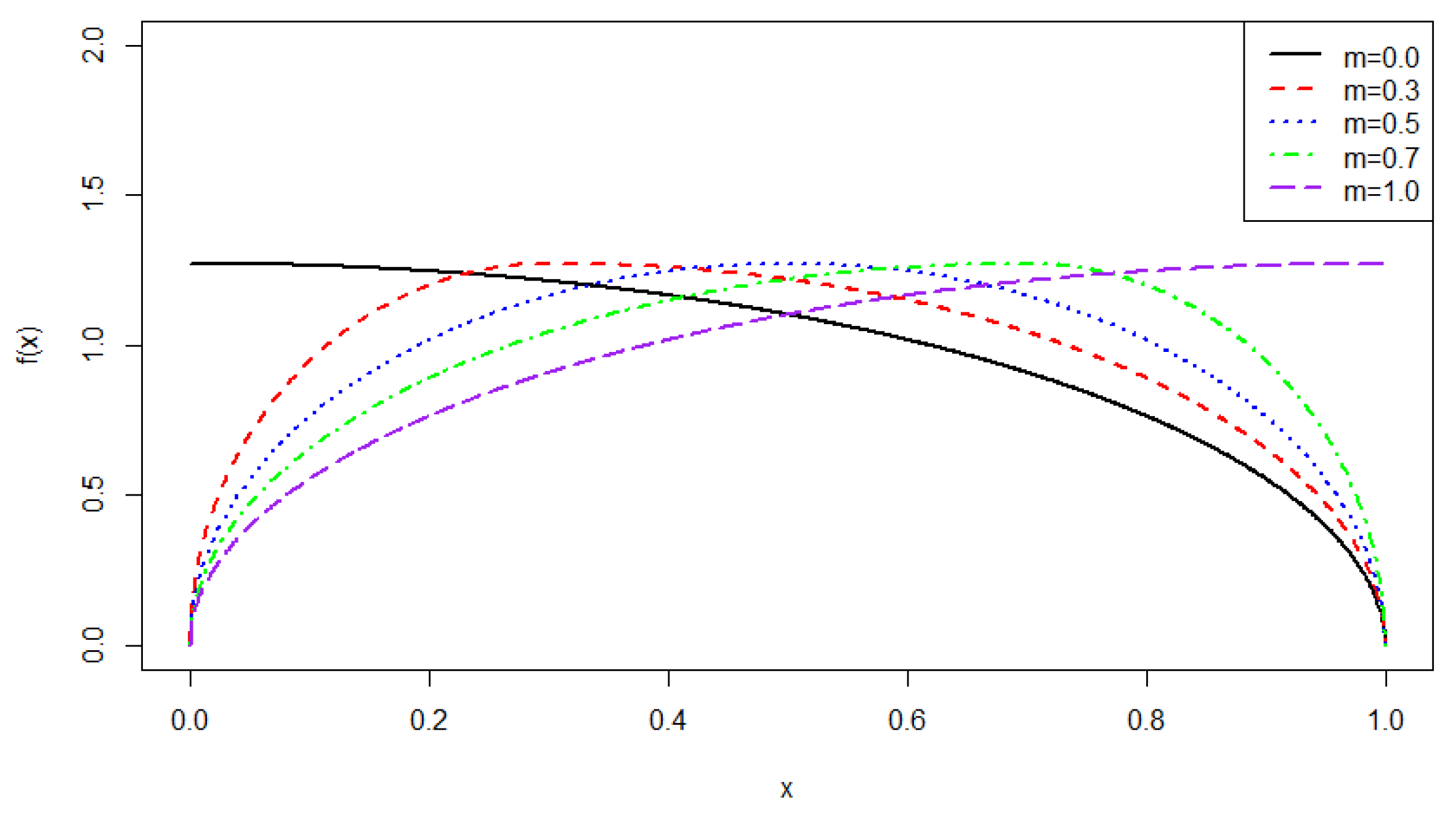
Figure 2.
Cumulative distribution functions of distributions for different choices of m: .

Figure 3.
Density plots of true beta distribution with the bi-elliptical fit and triangular fit:(a) and (b) .
Figure 3.
Density plots of true beta distribution with the bi-elliptical fit and triangular fit:(a) and (b) .

| (a) | (b) |

Table 1.
Performance measures of parameter estimation. Here is the true parameter and is the estimator and are the estimates. Here .
Table 1.
Performance measures of parameter estimation. Here is the true parameter and is the estimator and are the estimates. Here .
| Measure | Definition | Estimate |
|---|---|---|
| Bias | ||
| Empirical Standard Error (Empirical SE) | ||
| Mean Square Error(MSE) | ||
| Root Mean Square Error (RMSE) |
Table 2.
One-parameter estimation
| Size | Bias | Empirical SE | MSE | RMSE | |
|---|---|---|---|---|---|
| m=0.3 | 200 | 0.0118 | 0.1101 | 0.0122 | 0.1107 |
| 400 | 0.0045 | 0.0762 | 0.0058 | 0.0763 | |
| 600 | 0.0038 | 0.0650 | 0.0042 | 0.0651 | |
| 800 | 0.0035 | 0.0584 | 0.0034 | 0.0585 | |
| 1000 | -0.0002 | 0.0474 | 0.0022 | 0.0474 | |
| m=0.5 | 200 | 0.0031 | 0.1179 | 0.0139 | 0.1178 |
| 400 | -0.0030 | 0.0803 | 0.0064 | 0.0803 | |
| 600 | -0.0017 | 0.0651 | 0.0042 | 0.0651 | |
| 800 | -0.0006 | 0.0621 | 0.0038 | 0.0620 | |
| 1000 | -0.0005 | 0.0559 | 0.0031 | 0.0559 | |
| m=0.7 | 200 | -0.0029 | 0.1109 | 0.0123 | 0.1109 |
| 400 | -0.0054 | 0.0782 | 0.0061 | 0.0783 | |
| 600 | -0.0041 | 0.0636 | 0.0041 | 0.0637 | |
| 800 | -0.0019 | 0.0529 | 0.0028 | 0.0529 | |
| 1000 | -0.0012 | 0.0485 | 0.0023 | 0.0485 |
Table 3.
Three-parameter estimation
| Size | Bias | Empirical SE | MSE | RMSE | |
|---|---|---|---|---|---|
| a=-1 | 200 | 0.0416 | 0.0601 | 0.0041 | 0.0641 |
| 400 | 0.0268 | 0.0375 | 0.0016 | 0.0405 | |
| 600 | 0.0192 | 0.0288 | 0.0009 | 0.0304 | |
| 800 | 0.0148 | 0.0238 | 0.0006 | 0.0246 | |
| 1000 | 0.0127 | 0.0184 | 0.0004 | 0.0196 | |
| b=5 | 200 | -0.0540 | 0.0807 | 0.0072 | 0.0851 |
| 400 | -0.0343 | 0.0543 | 0.0032 | 0.0563 | |
| 600 | -0.0216 | 0.0373 | 0.0014 | 0.0378 | |
| 800 | -0.0172 | 0.0331 | 0.0011 | 0.0327 | |
| 1000 | -0.0165 | 0.0289 | 0.0009 | 0.0292 | |
| m=0.3 | 200 | 0.0425 | 0.6818 | 0.3573 | 0.5978 |
| 400 | -0.0378 | 0.4645 | 0.1669 | 0.4085 | |
| 600 | -0.0383 | 0.3841 | 0.1145 | 0.3384 | |
| 800 | -0.0318 | 0.3139 | 0.0765 | 0.2766 | |
| 1000 | -0.0279 | 0.2783 | 0.0601 | 0.2452 |
Table 4.
Comparing the bi-elliptic and triangular distribution as a proxy for the beta distribution.
Table 4.
Comparing the bi-elliptic and triangular distribution as a proxy for the beta distribution.
| 1 | 1.2 | 1.4 | 1.6 | 1.8 | 2 | 2.5 | 3 | 3.5 | ||
|---|---|---|---|---|---|---|---|---|---|---|
| AIC_be | 10.066 | 1.918 | -6.733 | -14.623 | -22.296 | -29.908 | -45.229 | -61.163 | -74.815 | |
| AIC_t | 23.765 | 13.193 | 0.262 | -11.879 | -23.828 | -35.026 | -57.999 | -79.103 | -96.519 | |
| % | 99% | 99% | 92% | 68% | 39% | 20% | 4% | 0.70% | 0.50% | |
| r | 99% | 97% | 87% | 65% | 41% | 23% | 5% | 2% | 0.90% | |
| AIC_be | 6.173 | 3.081 | -2.514 | -10.034 | -16.564 | -23.794 | -39.446 | -54.045 | -67.704 | |
| AIC_t | 17.767 | 14.166 | 7.386 | -3.13 | -12.592 | -22.43 | -44.675 | -64.882 | -82.487 | |
| % | 95% | 96% | 99% | 91% | 77% | 61% | 22% | 8% | 4% | |
| r | 94% | 97% | 96% | 87% | 73% | 58% | 24% | 9% | 4% | |
| AIC_be | -1.700 | -1.610 | -3.815 | -8.597 | -14.277 | -19.959 | -34.647 | -48.833 | -62.024 | |
| AIC_t | 4.162 | 7.042 | 4.775 | -1.359 | -8.858 | -16.679 | -36.352 | -54.951 | -71.696 | |
| % | 84% | 96% | 97% | 94% | 85% | 72% | 38% | 18% | 10% | |
| r | 81% | 93% | 93% | 90% | 81% | 70% | 40% | 21% | 12% | |
| AIC_be | -8.647 | -7.736 | -8.192 | -10.410 | -14.568 | -19.127 | -31.892 | -44.586 | -57.418 | |
| AIC_t | -6.283 | -2.150 | -1.422 | -4.286 | -9.734 | -15.477 | -32.175 | -48.420 | -64.392 | |
| % | 66% | 88% | 93% | 91% | 86% | 78% | 49% | 28% | 16% | |
| r | 62% | 82% | 88% | 86% | 80% | 73% | 49% | 30% | 19% | |
| AIC_be | -17.017 | -14.320 | -13.379 | -14.247 | -16.075 | -20.384 | -30.409 | -42.249 | -53.422 | |
| AIC_t | -18.339 | -11.950 | -8.839 | -9.589 | -11.858 | -17.318 | -30.354 | -44.83 | -58.678 | |
| % | 40% | 70% | 82% | 85% | 82% | 74% | 50% | 33% | 21% | |
| r | 42% | 67% | 78% | 79% | 77% | 70% | 50% | 36% | 24% | |
| AIC_be | -24.240 | -21.475 | -19.367 | -18.221 | -20.012 | -22.113 | -31.092 | -41.352 | -51.936 | |
| AIC_t | -27.151 | -21.733 | -16.687 | -14.860 | -17.067 | -19.831 | -30.899 | -43.639 | -56.88 | |
| % | 24% | 52% | 71% | 77% | 72% | 68% | 53% | 35% | 21% | |
| r | 28% | 51% | 67% | 73% | 69% | 65% | 52% | 37% | 25% | |
| AIC_be | -61.550 | -53.756 | -47.594 | -44.105 | -41.357 | -40.748 | -42.803 | -47.288 | -53.401 | |
| AIC_t | -76.637 | -65.648 | -55.050 | -48.96 | -45.003 | -43.972 | -45.472 | -50.903 | -58.258 | |
| % | 6% | 7% | 14% | 22% | 26% | 31% | 30% | 25% | 21% | |
| r | 7% | 9% | 17% | 25% | 31% | 32% | 34% | 29% | 24% | |
| AIC_be | -75.059 | -68.325 | -60.512 | -55.512 | -53.495 | -50.528 | -50.604 | -53.617 | -57.843 | |
| AIC_t | -88.337 | -84.029 | -72.241 | -64.083 | -60.338 | -56.246 | -55.619 | -58.229 | -63.477 | |
| % | 1.50% | 4% | 7% | 13% | 14% | 20% | 22% | 22% | 20% | |
| r | 1.50% | 6% | 10% | 15% | 17% | 22% | 25% | 25% | 22% | |
| AIC_be | -89.653 | -82.796 | -72.130 | -67.252 | -63.540 | -60.938 | -59.210 | -60.364 | -62.992 | |
| AIC_t | -114.394 | -101.53 | -88.022 | -78.783 | -72.639 | -68.977 | -65.661 | -66.351 | -69.603 | |
| % | 0.20% | 6% | 5% | 8% | 10% | 12% | 17% | 17% | 15% | |
| r | 0.70% | 7% | 6% | 10% | 12% | 16% | 19% | 20% | 18% |
Disclaimer/Publisher’s Note: The statements, opinions and data contained in all publications are solely those of the individual author(s) and contributor(s) and not of MDPI and/or the editor(s). MDPI and/or the editor(s) disclaim responsibility for any injury to people or property resulting from any ideas, methods, instructions or products referred to in the content. |
© 2025 by the authors. Licensee MDPI, Basel, Switzerland. This article is an open access article distributed under the terms and conditions of the Creative Commons Attribution (CC BY) license (http://creativecommons.org/licenses/by/4.0/).
Copyright: This open access article is published under a Creative Commons CC BY 4.0 license, which permit the free download, distribution, and reuse, provided that the author and preprint are cited in any reuse.


