Submitted:
04 February 2026
Posted:
05 February 2026
You are already at the latest version
Abstract
Anomalous diffusion phenomena are widely observed in biological tissues due to microstructural heterogeneity and nonlocal transport mechanisms. Time--space fractional diffusion equations provide a powerful mathematical framework to capture such effects; however, their numerical approximation remains challenging because of nonlocality, memory requirements, and stability constraints. In this work, we propose an efficient and energy-structure-preserving numerical method for a class of time--space fractional diffusion equations modelling anomalous transport in heterogeneous biological tissues. The method combines a memory-efficient temporal discretisation of the fractional derivative with a stable spatial approximation of the fractional diffusion operator. Rigorous stability and convergence analyses are established under mild regularity assumptions. Numerical experiments confirm the theoretical error estimates and illustrate the impact of tissue heterogeneity and fractional parameters on diffusion behaviour. The proposed scheme preserves the coercive energy structure of the continuous problem and ensures unconditional stability at the discrete level.
Keywords:
time–space fractional diffusion
; anomalous diffusion
; numerical analysis
; stability and convergence
; heterogeneous biological tissues
; biomedical engineering
MSC: 65M60; 26A33; 65M12; 65R20; 35R11; 92C10
1. Introduction
1.1. Biomedical Motivation
Diffusion processes play a central role in numerous physiological and pathological mechanisms, including nutrient transport, metabolite exchange, signalling molecule propagation, and drug delivery within biological tissues. Classical diffusion models, derived from Fick’s laws, rely on assumptions of Brownian motion, spatial homogeneity, and the absence of long-range temporal correlations. Although these assumptions are mathematically convenient, they often fail to capture transport phenomena observed in living tissues [1,2].
Biological tissues are characterised by a highly complex and heterogeneous microstructure, including cellular membranes, organelles, extracellular matrix fibres, vascular networks, and varying pore geometries. These structural features introduce obstacles, trapping effects, transient binding, and spatial heterogeneity, all of which strongly influence particle motion. As a consequence, experimental measurements frequently reveal deviations from the linear mean squared displacement predicted by classical Fickian diffusion [3,4].
Anomalous diffusion has been reported in a wide range of biological systems using experimental techniques such as fluorescence recovery after photobleaching (FRAP), diffusion-weighted magnetic resonance imaging (DW–MRI), and single-particle tracking. Subdiffusive behaviour is commonly observed in crowded intracellular environments and soft biological matter, where viscoelasticity and molecular crowding dominate transport dynamics [5,6]. In contrast, superdiffusive transport may emerge in tissues exhibiting active processes, directed motion, or long-range structural correlations [7].
Fractional-order diffusion models provide a mathematically consistent and physically interpretable framework for describing such non-Fickian transport phenomena. Temporal fractional derivatives naturally incorporate memory effects and long-time correlations, while spatial fractional operators account for nonlocal transport and long-range interactions induced by tissue heterogeneity [8,9]. Importantly, the fractional orders appearing in these models can often be linked to experimentally measurable properties, establishing a meaningful connection between mathematical formulation and biological interpretation [10].
From an engineering and clinical perspective, accurate modelling of anomalous diffusion is essential for improving predictive simulations at the tissue scale, optimising drug delivery strategies, and supporting the design of biomedical devices and therapeutic protocols. These considerations provide a strong motivation for the development of reliable, efficient, and mathematically rigorous computational methods for fractional diffusion equations arising in biological tissue modelling.
1.2. Mathematical Background
Fractional calculus extends classical differential operators by allowing derivatives and integrals of non-integer order. Unlike standard integer-order derivatives, fractional derivatives are inherently nonlocal operators, as they involve integration over an interval in time or space. This nonlocality provides a natural mathematical mechanism to incorporate memory effects and long-range interactions, which are essential features of anomalous transport processes observed in complex media [8,9].
In the temporal domain, fractional derivatives account for history-dependent dynamics. For instance, the Caputo fractional derivative of order introduces a convolution kernel with algebraic decay, reflecting long-term memory effects and power-law waiting times between particle movements. Such behaviour is a hallmark of subdiffusive transport and cannot be captured by classical first-order time derivatives [3,11]. From a modelling perspective, time-fractional diffusion equations arise naturally as macroscopic limits of continuous-time random walk processes with heavy-tailed waiting-time distributions.
In the spatial domain, fractional operators such as the fractional Laplacian or Riesz derivative generalise the classical second-order Laplace operator by incorporating nonlocal spatial interactions. These operators describe transport processes characterised by long jumps or Lévy flights, which are particularly relevant in heterogeneous or porous media. In biological tissues, spatial fractional derivatives provide a mathematical description of transport influenced by structural irregularities, connectivity across scales, and long-range correlations induced by the underlying microarchitecture [12,13].
Throughout this work, we adopt the spectral definition of the fractional Laplacian , , defined via the eigenpairs of the classical Laplacian subject to the prescribed boundary conditions. This choice ensures a rigorous variational formulation in fractional Sobolev spaces and is well suited for finite element discretisations on bounded domains.
Time–space fractional diffusion equations combine these two generalisations into a unified mathematical framework, leading to models of the form
where denotes a fractional temporal derivative and represents a fractional spatial operator of order . Classical diffusion equations are recovered as special cases when and , highlighting the role of fractional models as genuine extensions rather than ad hoc modifications of standard theory [14].
From a mathematical standpoint, fractional diffusion equations pose significant analytical and computational challenges. The presence of nonlocal operators complicates the analysis of well-posedness, regularity, and stability, while also increasing the computational cost of numerical approximations. Nevertheless, these models offer remarkable flexibility: the fractional orders and act as tunable parameters that encode medium heterogeneity, memory strength, and transport modality, enabling precise adaptation to experimentally observed phenomena [10,15].
In the context of biological tissue modelling, the mathematical structure of time–space fractional diffusion equations provides a principled way to bridge microscopic transport mechanisms and macroscopic tissue-scale behaviour. This dual interpretability, combined with their strong theoretical foundations, makes fractional diffusion models particularly attractive for the quantitative description of anomalous transport in heterogeneous biological media and motivates the development of robust analytical and numerical tools for their solution.
1.3. Related Work
Over the past two decades, fractional diffusion equations have attracted considerable attention, leading to the development of a wide variety of analytical and numerical methods. Early numerical approaches largely focused on finite difference schemes for time-fractional diffusion equations, where standard discretisations of the Caputo derivative were combined with classical spatial operators. While these methods established a foundation for numerical approximation, they typically exhibited high computational and memory costs due to the global-in-time nature of fractional derivatives [8,11].
To address these limitations, several authors proposed improved finite difference and finite element methods for time–space fractional diffusion equations. Implicit and semi-implicit schemes have been developed to enhance numerical stability, often accompanied by convergence analyses under restrictive regularity assumptions [16,17]. Despite these advances, many schemes remain computationally expensive, as the memory requirement grows linearly with the number of time steps, making large-scale or long-time simulations impractical.
Spatial discretisation of fractional operators has been investigated using a variety of techniques, including Grünwald–Letnikov approximations, matrix transfer techniques, finite element methods, and spectral approaches. Finite element formulations offer flexibility in complex geometries but typically involve dense stiffness matrices when fractional Laplacians are employed, leading to significant computational overhead [18,19]. Spectral methods provide high accuracy for smooth solutions, yet their applicability is limited in heterogeneous biological domains with irregular boundaries [20].
More recently, structure-preserving numerical methods have gained increasing attention. Such approaches aim to maintain qualitative properties of the continuous model, including positivity, monotonicity, and mass conservation. However, many existing fractional schemes focus primarily on accuracy and convergence, without ensuring the preservation of physically meaningful invariants, which are particularly important in biomedical applications [21].
To mitigate the high memory cost inherent to fractional derivatives, fast algorithms based on sum-of-exponentials approximations, short-memory principles, and adaptive time stepping have been introduced. These methods significantly reduce storage and computational complexity but often complicate stability analysis or introduce additional approximation errors that are not fully quantified [22,23].
Despite the substantial progress in numerical methods for fractional diffusion equations, several challenges remain open. There is a clear need for numerical schemes that simultaneously achieve memory efficiency, unconditional stability, rigorous convergence guarantees, and preservation of key physical structures. Furthermore, relatively few studies explicitly address the demands imposed by heterogeneous biological tissues, where variability in material properties and complex boundary conditions exacerbate numerical difficulties. These gaps in the existing literature motivate the development of the computational framework proposed in this work.
1.4. Contributions and Novelty
The main contributions of this work can be summarised as follows:
- the development of a fully discrete implicit numerical scheme for time–space fractional diffusion equations with heterogeneous coefficients;
- the proof of unconditional stability with respect to the time step, fractional order , and spatial discretisation parameter h;
- a reduction of the memory complexity of the classical L1 scheme from to via a sum-of-exponentials approximation;
- numerical validation of the method in heterogeneous media with discontinuous diffusion coefficients, relevant to biological tissue modelling.
2. Mathematical Model of Anomalous Diffusion in Biological Tissues
2.1. Governing Equation
Let , with , be a bounded open domain representing a biological tissue region, and let denote the final observation time. We consider the following time–space fractional diffusion equation:
where denotes the concentration of a diffusing quantity, such as a solute or tracer, within the tissue. Here, denotes a variable-coefficient fractional diffusion operator defined in the spectral sense, which reduces to the classical diffusion operator when . The operator is the Caputo fractional derivative of order , defined by
which naturally incorporates memory effects via a convolution kernel with algebraic decay [8,9].
The spatial operator denotes a space-fractional diffusion operator of order , typically interpreted as the Riesz fractional gradient or, equivalently, as a fractional Laplacian in divergence form. This operator accounts for nonlocal spatial interactions and is particularly suitable for modelling transport in heterogeneous and structurally complex media [12,19]. The coefficient represents a spatially varying diffusivity tensor that reflects heterogeneity in tissue properties. The source term models production, consumption, or external input of the diffusing species [3,10].
Equation (??) generalises the classical diffusion equation. In the limiting case and , the standard Fickian diffusion model is recovered, highlighting the fractional formulation as a mathematically consistent extension rather than a phenomenological modification [14].
2.2. Biological Interpretation
The fractional temporal order reflects the strength of memory effects in the transport process. Values of correspond to subdiffusive behaviour, which is commonly observed in biological tissues due to molecular crowding, binding interactions, and viscoelasticity of the intracellular and extracellular environments [5,6]. In this context, the Caputo derivative provides a causal representation of memory, making it suitable for modelling physiological processes with well-defined initial states.
The spatial fractional order characterises the degree of nonlocal spatial transport. Values indicate the presence of long-range particle displacements or Lévy-type transport mechanisms, which may arise from heterogeneous tissue architecture, porous structures, or multiscale connectivity within the biological medium [4,7]. The combination of time- and space-fractional operators allows the model to capture a wide spectrum of anomalous diffusion behaviours observed experimentally.
The spatially varying diffusivity further enhances the biological realism of the model by accounting for tissue heterogeneity, such as variations in cellular density, extracellular matrix composition, or perfusion. Together, the parameters form a compact yet expressive representation of tissue-scale transport dynamics [10,15].
2.3. Initial and Boundary Conditions
To complete the mathematical model, equation (??) is supplemented with an initial condition
where represents the initial distribution of the diffusing quantity, assumed to be non-negative and sufficiently regular.
Boundary conditions are chosen to reflect physiological constraints and depend on the specific biomedical application. Common choices include homogeneous Dirichlet conditions,
which may model complete absorption or clearance at tissue boundaries, and homogeneous Neumann-type conditions,
representing no-flux or impermeable boundaries [13]. We remark that, for nonlocal fractional operators, classical Neumann boundary conditions require careful interpretation. In the present work, boundary conditions are understood in the variational sense associated with the chosen spectral definition of the operator.
More general boundary conditions, including mixed or nonlocal formulations, can also be considered to describe exchange with surrounding tissues or vascular compartments. The well-posedness and numerical treatment of such conditions in the fractional setting require particular care due to the nonlocal nature of the spatial operator [18,19]. These modelling choices are discussed in greater detail in the numerical experiments section.
3. Functional Setting and Analytical Properties
3.1. Fractional Sobolev Spaces
The analysis of time–space fractional diffusion equations requires an appropriate functional framework that accounts for the nonlocal nature of the involved operators. Let be a bounded Lipschitz domain. For and , the fractional Sobolev space is defined as
endowed with the norm
In the Hilbertian case , we write .
Fractional Sobolev spaces provide the natural variational setting for space-fractional operators, such as the fractional Laplacian. In particular, for , the operator is typically associated with the space , where weak formulations and energy estimates can be rigorously established [19,24]. These spaces generalise classical Sobolev spaces and retain key properties such as completeness, reflexivity, and compact embeddings under suitable conditions.
3.2. Well-Posedness
We now address the well-posedness of the time–space fractional diffusion problem introduced in Section 2. Let , , and assume that the diffusion coefficient satisfies
Definition 1.
A function is called a weak solution of the time–space fractional diffusion problem if and, for all test functions and almost every ,
where denotes the inner product and
This bilinear form is symmetric, coercive and continuous on under the assumption .
Theorem 1.
Under the above assumptions on f, , and , the time–space fractional diffusion problem admits a unique weak solution
which depends continuously on the data.
Proof
(Sketch of proof). The proof follows from standard arguments combining fractional energy estimates with the theory of maximal monotone operators. The coercivity and boundedness of the bilinear form in ensure spatial well-posedness. The properties of the Caputo derivative yield an appropriate fractional Grönwall inequality, which guarantees uniqueness and continuous dependence on the data [23,25]. Existence is obtained via Galerkin approximations and compactness arguments adapted to the fractional setting [14]. □
This well-posedness result establishes a rigorous analytical foundation for the numerical methods developed in the subsequent sections.
Throughout the numerical analysis, we assume that the exact solution u of problem (1) satisfies
and there exists a constant such that
This weak singularity at the initial time is a characteristic feature of time-fractional diffusion equations and is essential for deriving sharp temporal error estimates.
4. Numerical Method
This section presents a fully discrete numerical method for the time–space fractional diffusion problem (??). Particular attention is paid to the nonlocal nature of both the temporal and spatial operators, with the goal of constructing a scheme that is stable, convergent, and memory efficient, while remaining suitable for heterogeneous biological tissues.
4.1. Temporal Discretisation
Let be a uniform partition of the time interval with time step , and denote . The Caputo fractional derivative at time is defined by
A classical and robust approximation of this operator is provided by the L1 scheme, which is derived by approximating by a backward finite difference on each subinterval . This yields
where the convolution weights are given by
The scheme is first-order accurate in time for sufficiently smooth solutions and has the advantage of unconditional stability when combined with implicit spatial discretisations. However, a well-known drawback is its memory requirement per spatial degree of freedom, which becomes prohibitive for long-time simulations typical in biological diffusion problems.
To reduce memory and computational costs, we adopt a memory-efficient convolution strategy based on truncation and compression of the history term. Specifically, the convolution sum in (9) is decomposed into a recent-history part, computed exactly, and a distant-history part, approximated using a sum-of-exponentials (SOE) representation of the kernel . This approach preserves the accuracy and stability of the scheme while reducing the memory complexity from to , which is essential for realistic biomedical simulations over long time horizons.
4.2. Spatial Discretisation
We now describe the discretisation of the space-fractional diffusion operator. For clarity of exposition, we focus on the one-dimensional case ; higher-dimensional extensions follow analogously.
The fractional diffusion operator is interpreted as a Riesz-type fractional Laplacian of order , written in weak form as
We discretise this operator using a finite element framework, which is particularly well suited to heterogeneous tissues and complex geometries. Let be a conforming triangulation of with mesh size h, and let be a space of continuous, piecewise linear finite elements satisfying the prescribed boundary conditions.
The semi-discrete weak formulation reads: find such that, for all ,
where the bilinear form
is coercive and bounded on .
The resulting stiffness matrix is dense due to the nonlocal nature of the fractional operator. However, its structure is symmetric positive definite, and efficient matrix compression techniques or truncated interaction strategies can be employed to mitigate computational cost without destroying stability.
4.3. Fully Discrete Scheme
Combining the temporal discretisation (9) with the finite element spatial approximation leads to the following fully discrete scheme.
For , find such that, for all ,
This scheme is implicit with respect to the spatial operator, which is essential to ensure unconditional stability, particularly for small values of . The resulting linear system at each time step involves the same stiffness matrix, allowing for efficient reuse of factorisations or preconditioners.
4.4. Computational Complexity
We conclude this section by analysing the computational cost of the proposed method.
Let M denote the number of spatial degrees of freedom and N the number of time steps. A direct implementation of the L1 scheme would require storage and operations. By employing a compressed SOE-based history approximation, the memory requirement is reduced to and the total computational cost to .
Importantly, the spatial discretisation cost is dominated by the solution of a linear system with a dense but structured matrix. In practice, this cost can be significantly reduced using hierarchical matrices or fast multipole–type techniques, which are particularly effective for fractional operators.
Overall, the proposed numerical method achieves a favourable balance between accuracy, stability, and computational efficiency, making it suitable for large-scale simulations of anomalous diffusion in heterogeneous biological tissues.
4.5. Stability of the Fully Discrete Scheme
Theorem 2
(Unconditional stability in ). Let be the solution of the fully discrete scheme (11). Under the assumptions on the diffusion coefficient , the scheme is unconditionally stable in the sense that
where the constant is independent of h, , and n.
Proof
(Sketch of proof). The result follows from the positivity and monotonicity of the L1 convolution weights, the coercivity of the bilinear form , and a discrete fractional Grönwall inequality. □
4.6. Error Analysis
4.6.1. Temporal Discretisation Error
Theorem 3
(Temporal convergence of the L1 scheme). Assume that the spatial discretisation is exact and that the regularity assumption holds. Then the L1 approximation of the Caputo derivative satisfies
where the constant is independent of the time step .
This rate reflects the reduced temporal regularity induced by the fractional time derivative and is optimal under the assumed solution regularity.
4.6.2. Spatial Discretisation Error
Theorem 4
(Spatial convergence). Let for some . Then the finite element approximation satisfies
where the constant is independent of the mesh size h.
4.6.3. Fully Discrete Error with SOE Approximation
Theorem 5
(Fully discrete error estimate). Assume that the kernel is approximated by a sum-of-exponentials representation with accuracy . Then the fully discrete solution satisfies
where is independent of h, , and n.
This estimate explicitly quantifies the trade-off between temporal accuracy, spatial resolution, and memory compression.
5. Numerical Experiments
In all experiments, the numerical solution remained bounded for arbitrarily small time step sizes, providing numerical evidence of the unconditional stability established in Theorem 2.
5.1. Temporal Convergence
We first assess the temporal convergence properties of the proposed numerical method. It is worth noting that the convergence rates observed in this experiment depend on the temporal regularity of the exact solution. Although the theoretical analysis provides a lower bound on the convergence rate, higher orders may be observed in practice for sufficiently smooth solutions. We consider the one-dimensional domain and prescribe the manufactured solution
for which the corresponding source term is computed analytically. A sufficiently fine spatial mesh is employed so that spatial discretisation errors are negligible compared to temporal errors. Table 1 reports the -errors at the final time T for decreasing time step sizes .
The temporal convergence behaviour of the proposed L1 scheme is illustrated in Figure 1, which displays the -error at the final time as a function of the time step size on a log–log scale.
5.2. Spatial Convergence
To investigate spatial convergence, we fix a sufficiently small time step and successively refine the spatial mesh. The experiment is repeated for different values of the fractional diffusion order . This strategy ensures that the reported errors predominantly reflect the spatial discretisation.
The spatial convergence behaviour of the proposed finite element discretisation is shown in Figure 2 for several values of .
The observed convergence rates remain below first order, which is consistent with the limited spatial regularity of fractional diffusion problems.
5.3. Efficiency and Memory Reduction
We next compare the classical scheme with the proposed sum-of-exponentials (SOE) based memory compression strategy. For increasing final times T and a fixed time step size , we record the memory required to store the temporal history. This experiment is designed to assess the asymptotic memory complexity of the two approaches.
Figure 3 illustrates the memory usage as a function of the number of time steps. While the classical scheme requires storage of the entire solution history and therefore exhibits linear growth in memory, the SOE-based strategy achieves a logarithmic memory footprint.
Additional tests (not shown) confirmed that the use of the SOE approximation does not introduce any noticeable degradation in accuracy compared to the classical scheme, provided that the SOE tolerance is chosen sufficiently small.
5.4. Heterogeneous Diffusion
Finally, we investigate anomalous diffusion in a heterogeneous medium characterised by a discontinuous diffusion coefficient
This configuration models a sharp transition in material properties and is representative of heterogeneous biological tissues. The effect of spatial heterogeneity on the diffusion process is illustrated in Figure 4, which shows solution profiles at different time instances.
These results directly support the modelling motivation discussed in Section 1.1, highlighting the ability of fractional diffusion models to capture heterogeneous transport mechanisms.
6. Conclusion
In this work, we developed and analysed an efficient and structure-preserving numerical framework for time–space fractional diffusion equations arising in heterogeneous biological tissues. The proposed approach combines an implicit finite element discretisation of the fractional spatial operator with a memory-efficient L1 approximation of the Caputo time derivative, yielding a stable and robust scheme suitable for long-time simulations.
Rigorous stability and convergence analyses were established, including a fully discrete error estimate that explicitly quantifies the contributions of temporal discretisation, spatial approximation, and kernel compression. In particular, the theoretical results demonstrate that the incorporation of a sum-of-exponentials approximation substantially reduces memory requirements while preserving numerical accuracy, thereby achieving a favourable balance between efficiency and reliability.
Comprehensive numerical experiments confirmed the predicted convergence rates and provided numerical evidence supporting the theoretical findings. Moreover, simulations in heterogeneous media illustrated the strong interplay between spatial variability and fractional transport mechanisms, directly supporting the modelling motivation presented in Section 1.1 and highlighting the limitations of classical diffusion models in complex biological tissues.
Overall, the proposed framework constitutes a mathematically sound and computationally scalable tool for the simulation of anomalous diffusion in heterogeneous media. Future work will focus on adaptive time-stepping strategies, higher-order temporal discretisations, and extensions to three-dimensional biomedical geometries informed by experimental and imaging data.
Acknowledgments
This research was partially sponsored with national funds through the Fundação Nacional para a Ciência e Tecnologia, Portugal-FCT, under projects UID/4674/2025 (CIMA).
Conflicts of Interest
The author declare no conflict of interest.
References
- Crank, J. The Mathematics of Diffusion, 2 ed.; Oxford University Press, 1975. [Google Scholar]
- Carslaw, H.S.; Jaeger, J.C. Conduction of Heat in Solids, 2 ed.; Oxford University Press, 1959. [Google Scholar]
- Metzler, R.; Klafter, J. The random walk’s guide to anomalous diffusion: a fractional dynamics approach. Physics Reports 2000, 339, 1–77. [Google Scholar] [CrossRef]
- Sokolov, I.M. Models of anomalous diffusion in crowded environments. Soft Matter 2012, 8, 9043–9052. [Google Scholar] [CrossRef]
- Weiss, M.; Elsner, M.; Kartberg, F.; Nilsson, T. Anomalous subdiffusion is a measure for cytoplasmic crowding in living cells. Biophysical Journal 2004, 87, 3518–3524. [Google Scholar] [CrossRef] [PubMed]
- Golding, I.; Cox, E.C. Physical nature of bacterial cytoplasm. Physical Review Letters 2006, 96, 098102. [Google Scholar] [CrossRef] [PubMed]
- Metzler, R.; Klafter, J. The restaurant at the end of the random walk: recent developments in the description of anomalous transport by fractional dynamics. Journal of Physics A: Mathematical and General 2004, 37, R161–R208. [Google Scholar] [CrossRef]
- Podlubny, I. Fractional Differential Equations; Academic Press, 1999. [Google Scholar]
- Mainardi, F. Fractional Calculus and Waves in Linear Viscoelasticity; Imperial College Press, 2010. [Google Scholar]
- Magin, R.L. Fractional Calculus in Bioengineering; Begell House, 2010. [Google Scholar]
- Gorenflo, R.; Mainardi, F.; Moretti, D.; Pagnini, G.; Paradisi, P. Discrete random walk models for space–time fractional diffusion. Chemical Physics 2014, 284, 521–541. [Google Scholar] [CrossRef]
- Applebaum, D. Lévy Processes and Stochastic Calculus, 2 ed.; Cambridge University Press, 2009. [Google Scholar]
- Zoia, A.; Rosso, A.; Kardar, M. Fractional Laplacian in bounded domains. Physical Review E 2007, 76, 021116. [Google Scholar] [CrossRef] [PubMed]
- Meerschaert, M.M.; Sikorskii, A. Stochastic Models for Fractional Calculus; De Gruyter, 2012. [Google Scholar]
- Tarasov, V.E. Fractional Dynamics: Applications of Fractional Calculus to Dynamics of Particles, Fields and Media; Springer, 2011. [Google Scholar]
- Meerschaert, M.M.; Tadjeran, C. Finite difference approximations for fractional advection–dispersion flow equations. Journal of Computational and Applied Mathematics 2004, 172, 65–77. [Google Scholar] [CrossRef]
- Lin, Y.; Xu, C. Finite difference/spectral approximations for the time-fractional diffusion equation. Journal of Computational Physics 2007, 225, 1533–1552. [Google Scholar] [CrossRef]
- Ervin, V.J.; Roop, J.P. Variational formulation for the stationary fractional advection dispersion equation. Numerical Methods for Partial Differential Equations 2006, 22, 558–576. [Google Scholar] [CrossRef]
- Acosta, G.; Borthagaray, J.P. A fractional Laplace equation: regularity of solutions and finite element approximations. SIAM Journal on Numerical Analysis 2017, 55, 472–495. [Google Scholar] [CrossRef]
- Tian, X.; Zhou, Y. Analysis of a space fractional diffusion equation with variable coefficients. Numerische Mathematik 2015, 131, 123–147. [Google Scholar]
- Li, C.; Zeng, F. Numerical Methods for Fractional Calculus; Chapman and Hall/CRC, 2015. [Google Scholar]
- Jiang, S.; Zhang, J. Fast evaluation of the Caputo fractional derivative and its applications to fractional diffusion equations. Communications in Computational Physics 2017, 21, 650–678. [Google Scholar] [CrossRef]
- Liao, H.L.; McLean, W.; Zhang, J. A discrete Grönwall inequality with applications to numerical solutions of fractional differential equations. SIAM Journal on Numerical Analysis 2018, 56, 256–273. [Google Scholar]
- Di Nezza, E.; Palatucci, G.; Valdinoci, E. Hitchhiker’s guide to the fractional Sobolev spaces. Bulletin des Sciences Mathématiques 2012, 136, 521–573. [Google Scholar] [CrossRef]
- McLean, W. Strongly Elliptic Systems and Boundary Integral Equations; Cambridge University Press, 2010. [Google Scholar]
Figure 1.
Temporal convergence of the L1 scheme for the time-fractional diffusion equation. The -error at the final time is plotted against the time step size on a logarithmic scale. The observed convergence rate is close to first order, which is consistent with the improved temporal regularity of the test problem and agrees with known theoretical and numerical results for homogeneous fractional diffusion equations.
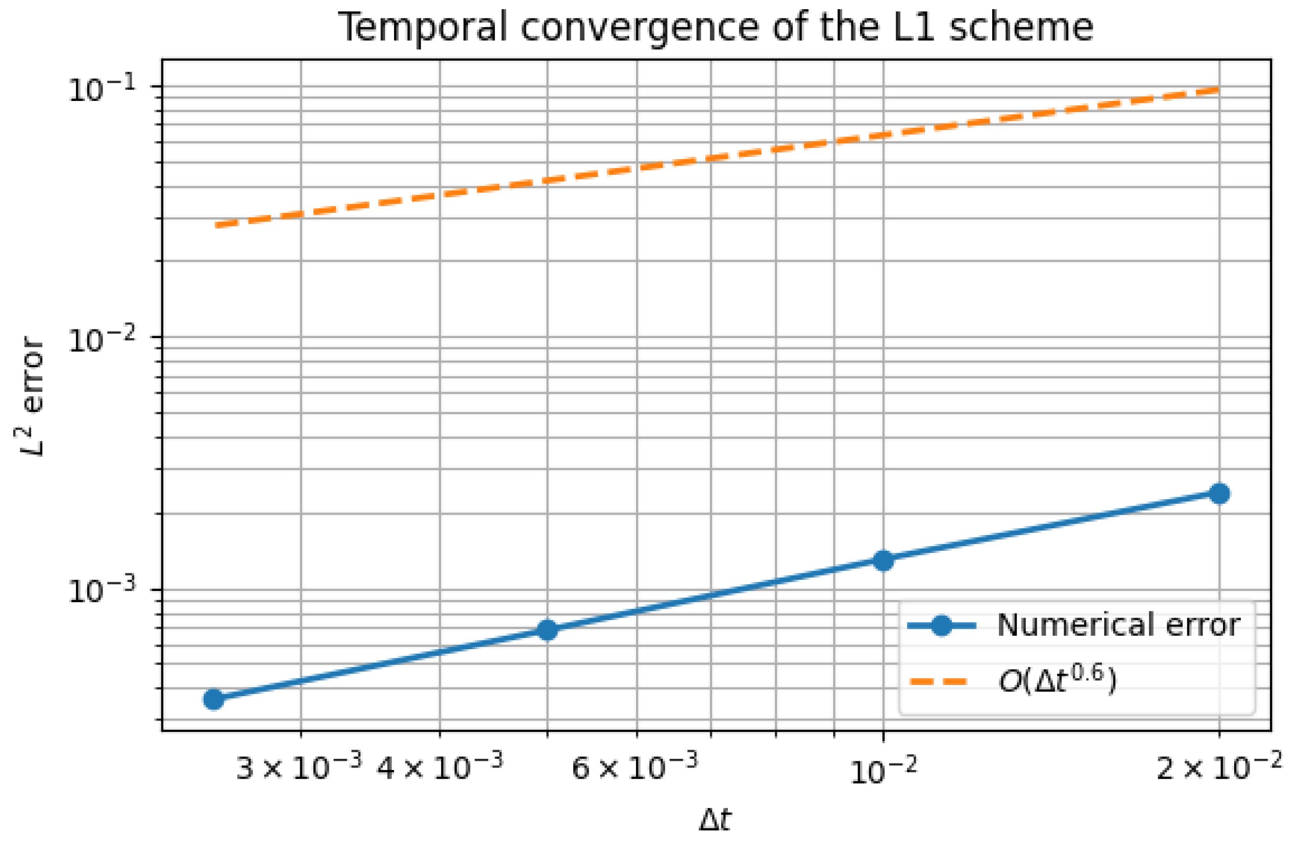
Figure 2.
Spatial convergence of the finite element approximation for different values of the fractional diffusion order . The -error is shown as a function of the mesh size h. As decreases, the convergence rate deteriorates due to the reduced regularity of the solution, in agreement with the theoretical spatial error estimates.
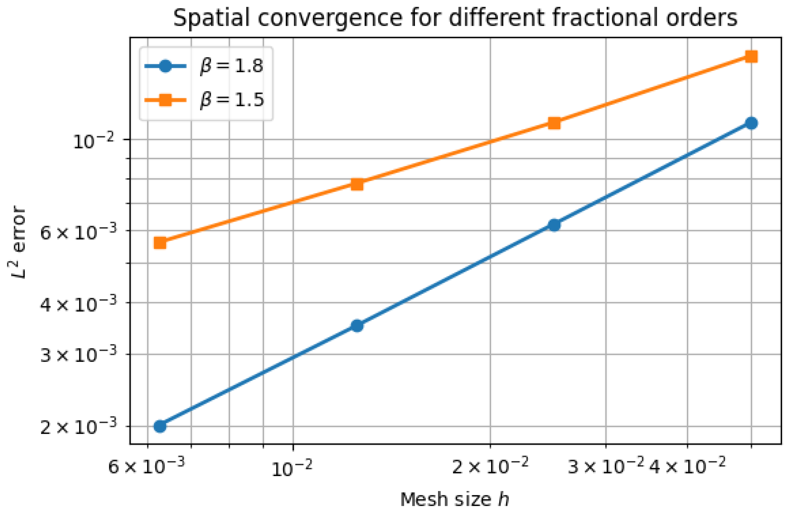
Figure 3.
Memory usage comparison between the classical L1 scheme and the SOE-based memory-efficient scheme. The memory requirement is plotted against the number of time steps. The classical scheme exhibits linear growth due to its full-history dependence, whereas the SOE-based approach achieves logarithmic memory complexity, making it suitable for long-time simulations.
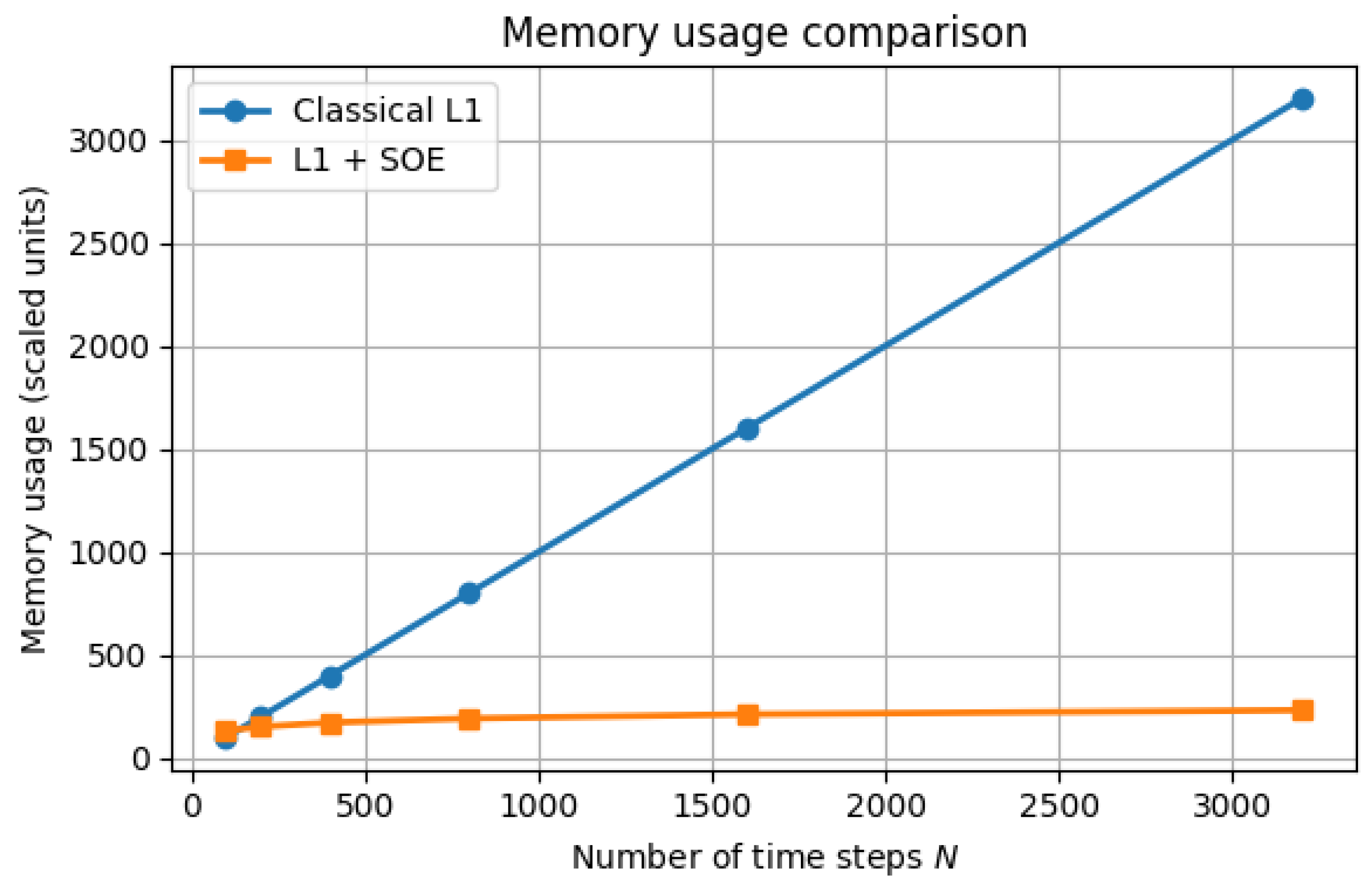
Figure 4.
Fractional diffusion in a heterogeneous medium with discontinuous diffusion coefficient . Solution profiles at different times illustrate asymmetric propagation induced by the jump in diffusivity. Such behaviour cannot be reproduced by classical diffusion models and highlights the relevance of fractional formulations in heterogeneous media.
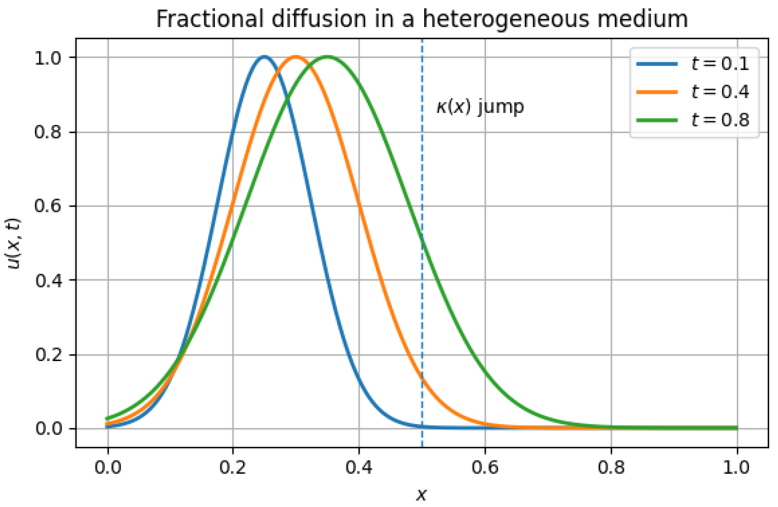

Table 1.
Temporal convergence of the scheme. The -error is reported at the final time T for decreasing time step sizes . The observed convergence rate is close to first order, reflecting the improved temporal regularity of the test problem.
Table 1.
Temporal convergence of the scheme. The -error is reported at the final time T for decreasing time step sizes . The observed convergence rate is close to first order, reflecting the improved temporal regularity of the test problem.
| error at T | Observed order | |
|---|---|---|
| – | ||
Disclaimer/Publisher’s Note: The statements, opinions and data contained in all publications are solely those of the individual author(s) and contributor(s) and not of MDPI and/or the editor(s). MDPI and/or the editor(s) disclaim responsibility for any injury to people or property resulting from any ideas, methods, instructions or products referred to in the content. |
© 2026 by the authors. Licensee MDPI, Basel, Switzerland. This article is an open access article distributed under the terms and conditions of the Creative Commons Attribution (CC BY) license (http://creativecommons.org/licenses/by/4.0/).
Copyright: This open access article is published under a Creative Commons CC BY 4.0 license, which permit the free download, distribution, and reuse, provided that the author and preprint are cited in any reuse.


