

Submitted:
01 July 2026
Posted:
03 July 2026
You are already at the latest version
Abstract
In the Kolmogorov Theory (KT) of consciousness, an algorithmic agent is an information-processing system that compresses sensory data into simpler models to plan actions that optimize an objective function, while operating under limited data access, finite computational resources, and the fundamental limits of algorithmic information theory (AIT). We show how these limitations naturally give rise to probability, Bayesian inference, precision, and emergence. Using a toy example of an agent compressing pages fromalarge library, we recover a weighted multi-model strategy in which probabilistic reasoning and Occam’s razor appear as the agent navigates between models. We then introduce precision—the confidence the agent assigns to its model relative to noisy data—as the second-order quantity that arbitrates the trade-off between trusting the prediction and trusting the observation. We formalize precision as inverse-variance weighting of prediction errors at the Comparator and show what it gives the agent: a principled model-updating process carried out by the Updater (a submodule of the Modeling Engine), in which a confidence-dependent gain determines how much each prediction error revises the model — so that reliable, persistent errors reshape the model while structureless errors are retained as residual noise, and structural learning saturates once the compressible regularity has been captured. We then connect the picture to Karl Friston’s Free Energy Principle and Active Inference, which appear as the variational-Bayesian special case of the bounded-agent story, and flag the main differences rather than collapsing the two. Finally, we propose a formal, agent-centric definition of emergence in terms of coarse-graining and Kolmogorov complexity, and connect it to cellular automata, the renormalization group, and partial models. The result is a unified account in which probability, precision, and emergence are all consequences of an agent’s drive to compress and model a noisy world under bounded resources.
Keywords:
algorithmicinformation theory
; algorithmic agent
; Bayesian inference
; precision
; prediction error
; attention
; gating
; free energy principle
; emergence
; coarse-graining
MSC: 68Q30; 94A15; 68T05
1. Introduction
“El universo (que otros llaman la Biblioteca)...”— Jorge Luis Borges, La biblioteca de Babel (1941)“The universe (which others call the Library)...”
Understanding how complex behaviors and probabilistic reasoning emerge from simple rules is a central challenge in both neuroscience and artificial intelligence. An alternative to starting from probability is provided by the Kolmogorov Theory (KT) of consciousness [1,2,3]. In this framework, the algorithmic agent interacts with its environment by compressing sensory data into simpler forms — by constructing models — to guide its actions toward increased valence [4,5]. Real agents, however, operate under inherent constraints: limited data access, finite computational resources, and noisy data.
Moreover, the uncomputability of Kolmogorov complexity means that agents cannot deduce the actual program (model) generating the data they receive. A foundational result in algorithmic information theory (AIT) — derived independently by Solomonoff, Kolmogorov, and Chaitin — states that there is no general algorithm that, given a string x, computes its exact Kolmogorov complexity , i.e., the length of the shortest program that outputs x on a fixed universal Turing machine [6]. The shortest model generating x cannot, in general, be found.
This paper shows how these limitations give rise to probability theory and Bayesian inference, to precision as a measure of confidence, and to the phenomenon of emergence [7,8,9]. We assume that agents seek to predict the world efficiently by finding short programs for data (under the Solomonoff prior) but are limited by (i) computational constraints (finite resources, uncomputability of K); (ii) partial, coarse-grained access to data; and (iii) noisy and incomplete data.
We make four contributions. First, we show that an ideal agent, driven by homeostatic goals, is naturally led to a weighted multi-model strategy with priors — essentially Bayesian inference — to interpret and predict its environment (Section 2). Second, and new to this revision, we introduce precision as the second-order quantity that governs how much a given mismatch between model and data should move the model, and show that it gives the Modeling Engine’s Updater a principled model-updating process: a confidence-weighted gain that decides, error by error, whether a mismatch revises the model or is retained as residual noise; we then tie precision to a concrete neural substrate in which attention and gating are limit cases of precision weighting (Section 3). Third, we connect the picture to the Free Energy Principle (FEP) and Active Inference, which appear as its variational-Bayesian special case, and flag the main differences (Section 4). Fourth, we formalize emergence through coarse-graining and Kolmogorov complexity, connecting it to cellular automata, the renormalization group, and partial models (Section 5Section 6).
The construction is inspired by Jaynes’s robot [10]. Like Jaynes, we treat probability as the calculus a rational agent must use under incomplete information; unlike his unbounded, purely epistemic robot, the algorithmic agent is resource-bounded and goal-directed. Probabilistic, multi-model inference emerges from its drive to compress once the Solomonoff prior is adopted as the AIT form of Occam’s razor, and — being telehomeostatic rather than purely inferential — the agent also carries an objective function, so that precision and action follow.
2. Bayesian Inference
Consider an agent tasked with modeling the world, which in KT is equivalent to being able to compress world data [4,11]. The agent needs a good predictive model for survival, and compression performance indicates predictive power under the Solomonoff prior [12,13]. The agent may use simple compressors such as gzip or sophisticated descendants such as large language models, which can also be used for compression [14,15].
The agent consists of three interacting modules (Figure 1) [3,4,5]: a Modeling Engine (ME), an Objective Function (OF), and a Planning Engine (PE). The ME’s primary goal is to find simple models of the world to predict the future and plan accordingly. The goal of the agent itself is to survive, to achieve “stasis” — a term covering both homeostasis (preservation of self) and telehomeostasis (preservation of kind).
Our first contribution is to show that a multi-model strategy (a “meta”-model), in which an agent maintains multiple models to balance compression efficiency against robustness to noise and data diversity, leads to better compression as the agent interacts with the world; and that this, combined with Solomonoff’s priors, naturally yields Bayesian inference and the emergence of probability, complemented by Occam’s razor.
2.1. A Multi-Model Strategy for Compression
Consider an agent sequentially fed pages from a large library, such as the Library of Congress (more than 32 million books in 470 languages). The agent aims to compress each newly arriving page as efficiently as possible, using the (meta)model built from past data, with only partial access: a model must be chosen after the first few lines of each page. Performance is measured by how well the agent compresses newly arriving data with the model it has built (Figure 2).
The agent begins by receiving a few pages, perhaps from a novel, and builds a simple model capturing their patterns (sentence structure, vocabulary). It uses this model to compress new pages, assuming they will be similar, while monitoring compression performance. When it later encounters a research paper that differs sharply from the novels, the existing model compresses poorly. The agent faces a decision: modify the current model to handle both, or maintain a separate model for research papers? What should it do with a page mixing English and Latin? It must contend with (a) partial, coarse-grained, sequential access; (b) diversity of content (languages, document types); and (c) noise (e.g., OCR errors, corrupted scans).
If the agent had immediate access to the entire corpus it could, in principle, build a single unified compressor. But it does not; a single holistic model is unlikely to be built rapidly under diversity and noise, and may be impossible to construct because it would have to include the process selecting the next book and page. An effective strategy for compressing future data is therefore to maintain a set of simpler submodels, each specialized to a content type, and to select the most appropriate one for each incoming page based on a notion of “probability”: given a new page, which models are more likely to apply?
To minimize the expected description length of future data, the compressor must trade off the observed frequency (probability) of models against their lengths (compression performance), reminiscent of Huffman coding, where more frequent symbols receive shorter codes [12]. This is essentially a Bayesian approach: assign probabilities to each model based on how well it compresses the data and how often it has been used, and update these probabilities as new data arrives by evaluating the likelihood of all data seen so far under each model. Thus an agent compressing both past and future data sequentially is naturally led to a probabilistic multi-model strategy. The framework generalizes to any objective function requiring a world model: whether the goal is stasis or prediction, the need to plan under uncertainty leads to a probabilistic, multi-model approach.
2.2. Occam’s Razor
An important feature of Bayesian inference is the use of priors. We have seen how priors arise from building multiple models and assessing how frequently they apply to past data. But why are simple models better? Solomonoff Induction provides a formal foundation. The probability of an observation is a weighted sum over all computable models that could generate the data, each weighted by its simplicity, measured by Kolmogorov complexity. The probability assigned to a model is
where is the length of the shortest program capable of generating the data. The preference for shorter programs follows from the hypothesis of a computational universe in which programs are generated at random (the “monkey typing” analogy): shorter self-terminating programs are statistically more probable, giving rise to the Solomonoff prior and formalizing Occam’s razor — among hypotheses that explain the data equally well, prefer the simplest.
One may also invoke an algorithmic form of natural selection in a computational soup: selection may favor agents that find simple models (easier to construct, store, and use) and agents that operate at a coarse-grained level of the world that can be modeled simply. The latter motivates the definition of emergence in Section 5.
3. Precision: Weighting the Model Against Noisy Data
Bayesian model selection (Section 2) tells the agent which model to trust; it does not yet say how strongly to trust a given observation relative to its current prediction. Real data are noisy, and the model is itself uncertain. When prediction and observation disagree, the agent must decide whether the mismatch is signal — evidence that the model is wrong and should be updated — or noise — a fluctuation to be tolerated. This arbitration is the role of precision.
3.1. Precision as Confidence-Weighted Updating
At the Comparator (Figure 1) the agent forms the prediction error between the bottom-up input (the data) and the top-down prediction . Both carry uncertainty; with variances , the precisions are the inverse variances and (high precision = high confidence). Combining prediction and observation, the posterior estimate is the prediction corrected by the error,
where the gain g sets the relative confidence between model and data: when the data are reliable () the gain and the agent follows the data; when the model is reliable () the gain and it holds its prediction, treating the mismatch as noise. This is the (scalar) Kalman gain [16]: predictive coding corresponds to Bayesian filtering, and in the linear-Gaussian limit to Kalman filtering [17].
What precision gives the agent is thus a principled model-updating process, carried out by the Updater — the submodule of the Modeling Engine that turns errors into model revisions. The same precision ratio acts at a slower timescale on the model itself,
with the confidence of the incoming evidence and that of the current model: reliable, persistent errors revise the model, structureless errors are left as residual. As the model accumulates structure, grows and ; further errors no longer drive structural change — though, in a noisy world, the residual remains and is still registered. The endpoint is the sufficient-statistic regime of Kolmogorov’s structure function, where the model has absorbed the compressible regularity and the remainder is random relative to it, (Section 5.3). Precision is therefore the mechanism by which the Modeling Engine distinguishes errors worth learning as structure from errors left as noise.
3.2. Attention and Gating as Limit Cases of Precision
If precision controls the gain on prediction errors, then attention and gating are naturally understood as the agent’s management of precision. In predictive coding, attention is the optimization of the precision assigned to selected prediction errors — a gain-control operation on error units [18]. Gating and routing are the limit cases: suppressing a channel is precision driven toward zero, amplifying a channel is precision driven high.
This has a concrete neural implementation: in the laminar neural mass model (LaNMM), cross-frequency coupling realizes the precision-weighted Comparator at the columnar level, with signal-envelope coupling computing the prediction error and envelope-envelope coupling implementing its precision-weighting (gating) [19].
4. Connection to Active Inference and the Free Energy Principle
The probabilistic, precision-weighted picture developed above connects naturally to Karl Friston’s Free Energy Principle (FEP) and Active Inference [17,20,21]. The relation is conservative: KT is a substrate-independent, algorithmic account of persistent agents, and FEP/AIF is its variational-Bayesian realization in the regime where a bounded agent performs approximate inference over hidden causes behind a Markov blanket [22]. We sketch the link and note the main differences; the full bridge is developed elsewhere [23,24].
The chain is short. A bounded agent cannot find the shortest program (Section 2), so it weights a model ensemble probabilistically; noisy data turn code length into negative log-likelihood, so the Comparator’s mismatch is scored by precision (Section 3); and once the agent must infer hidden causes z behind its sensory data x, using a tractable posterior in place of the exact , the natural objective is the variational free energy
an expected residual code length plus a cost for departing from the prior; minimizing it bounds the surprise while driving toward the true posterior. In this reading, Friston’s Markov blanket [25] is the probabilistic specialization of KT’s information membrane — external and internal states communicate only through sensory and active states — and the familiar predictive-coding and Kalman forms are its Gaussian corner, where the accuracy term reduces to the precision-weighted squared error of Section 3.
Two differences are worth highlighting as the story develops, rather than collapsing the frameworks. First, KT keeps the Objective Function separate: goals are a telehomeostatic valence the agent maximizes, and modeling, precision, and information-seeking are mechanisms serving it, whereas AIF folds goals into the generative model as prior preferences and reads behavior as free-energy minimization. Second, KT’s drive toward simplicity is algorithmic (), whereas FEP’s complexity term is prior-relative. These differences — and the exploration–exploitation regime in which they become operational — are developed in companion work [23,24]; here it suffices that FEP/AIF sits inside the bounded-agent picture as its variational-Bayesian special case.
5. Emergence
Emergence is central to understanding complex systems, where simple microscopic rules give rise to intricate macroscopic behavior [7,8,9]. We adopt an AIT approach in the KT setting, defining emergence in terms of Kolmogorov complexity and coarse-graining by agents. Our treatment is close in spirit to Khaleghi et al. [26], where emergence is characterized by data displaying several minimal partial models, but differs in the final definition, as clarified below.
Scope and companion paper. The full algorithmic-emergence theory—the weak/strong/algorithmic taxonomy, the thesis that compression is the hard part, and the result that the optimal coarse-graining of a system is not computable from its microdescription (“reduction is not construction”)—is developed in the dedicated companion paper [27]; the uncomputability reduction is machine-checked in Lean 4 (the KTAIT development / WP0195, https://github.com/giulioruffini/KTAIT). Here we use only the lightweight, agent-centric notion of emergence introduced below, which is what the probability and precision account of this paper requires.
5.1. Formal Definition in the Agent Framework
Recall that the Kolmogorov complexity of a dataset is the length of the shortest algorithm capable of reproducing it.

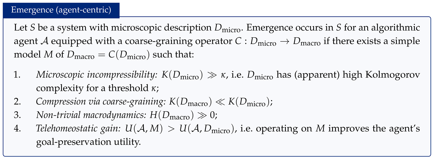
Let be a system with microscopic state space evolving under rules , generating a data sequence . The true Kolmogorov complexity is low if the system is governed by simple underlying rules, , where denotes string length. To an agent unaware of those rules, however, the data appear highly complex: the apparent complexity is . Let be a coarse-graining operator mapping the microscopic state space to a macroscopic one, with emergent rules and macroscopic data . Emergence occurs when: (i) the apparent complexity of is high; (ii) after coarse-graining, while the macroscopic entropy remains significant, ; and (iii) the coarse-graining is non-trivial, retaining mutual algorithmic information with the original system (a trivial map to a constant yields no emergence). In short, emergence reduces perceived complexity through coarse-graining while preserving high entropy and shared algorithmic information (Figure 3).
5.2. Cellular Automata and the Renormalization Group
Cellular automata (CA) exemplify how simple rules produce high apparent complexity at the microscopic level [9]. Rule 110 generates outputs that are highly complex and even Turing complete [28], yet coarse-graining can reveal periodic or self-similar macroscopic structure that is much simpler to describe. Israeli and Goldenfeld [29] showed that coarse-graining can transform elementary CA into new effective rules at a larger scale, revealing emergent phenomena not obvious microscopically — precisely our setting: microscopically high K, macroscopically compressible, with mutual algorithmic information preserved.
This parallels the Renormalization Group (RG) in statistical physics and field theory, which describes how a system’s behavior changes from microscopic to macroscopic scales by integrating out or averaging over microscopic degrees of freedom [30,31,32]. Under RG transformations, couplings flow toward fixed points representing scale-independent, emergent behavior whose universality is insensitive to microscopic detail — akin to emergent phenomena having lower Kolmogorov complexity than their underlying rules. From the algorithmic perspective, RG reduces apparent complexity by constructing an effective theory with fewer degrees of freedom, mirroring our definition of emergence.
5.3. Relation to Emergence Through Partial Models
Bédard and Bergeron [33] propose a closely related definition of emergence via Kolmogorov’s structure function; what they call partial models are, in fact, included in coarse-graining. An intuitive way to see the connection is to ask for the most compressed representation of a dataset achievable using only a bits. This is Kolmogorov’s structure function [12],
where x is a string of length n, S is a contemplated model (a set of n-length strings containing x), is the Kolmogorov complexity of S, and a bounds the complexity of S. As a increases, more structure can be captured and decreases. An accuracy-parameterized form measures the minimal description length of a model that fits x to within an error [34], capturing the trade-off between model simplicity and accuracy.
These ideas relate to effective complexity [8]: the Kolmogorov-optimal program splits into a part describing regularities (effective complexity) and a part capturing the structureless remainder (noise). This is the same split that the Updater’s precision-weighting governs in the noisy setting (Section 3.1): the gain on an error decides whether it is learned as regularity or left as noise. An agent limited in program length or computation explores coarse-grainings that produce drops in apparent complexity — effective regraining. In the agent framework, coarse-graining serves not only compression but stasis as dictated by the Objective Function; an agent may choose regrainings that are suboptimal for compression but advantageous for survival. Hence the two definitions are closely related but not equivalent.
6. Agent-Centric Definitions: Emergence and Complex Systems
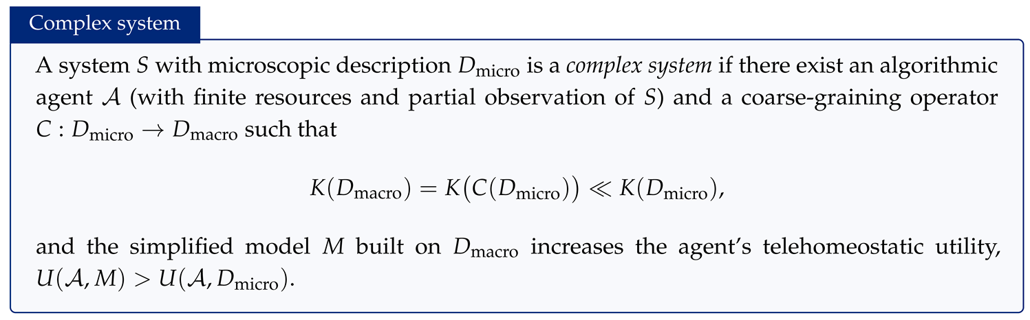
We now state the agent-centric definitions precisely. Here denotes Kolmogorov complexity, Shannon entropy, and the expected long-term preservation of agent ’s goal states (telehomeostatic utility).
7. Discussion
A key feature of this framework is that the agent must build and refine its models dynamically, “on the go,” as data arrive, with limited resources that drive it toward coarse-graining. The agent’s goal is not only to compress past data but to remain prepared for future data of a possibly different form, which requires a flexible, probabilistic modeling stance. When optimizing utility under uncertainty, it is generally more effective to use the full posterior over models than a single maximum a posteriori estimate, integrating expected utility across scenarios in line with decision theory [35].
Precision adds a second, orthogonal axis to this picture. Where Bayesian model selection chooses which model, precision sets how much each observation should move it — the confidence the agent places in its prediction relative to noisy data. Concretely, precision gives the Updater its model-updating process: reliable, persistent errors reshape the model while structureless errors are retained as residual noise, and structural learning saturates as the model converges toward a sufficient statistic for the compressible regularity in the data (Section 3.1). The same quantity has a concrete neural realization in cross-frequency coupling, where slow envelopes gate the gain of fast error channels, so that attention and gating become limit cases of precision control [19].
Multi-model strategies are widely used in machine learning. The Mixture of Experts framework trains specialized models and uses a gating network to select among them [36] — closely aligned with the multi-model approach here, and with precision-as-gating: the gate is, in effect, a precision assignment over experts. Ensemble learning combines independently trained models to improve robustness [37], and context-mixing compressors such as PAQ combine predictions from multiple context models [38]. The compositional nature of natural data further suggests hierarchical coarse-graining, consistent with findings in the visual [39,40] and auditory [41] primate systems. Finally, emergence is not merely a property of the data-generating system but also of the observing agent: the emergent behavior recognized depends on the coarse-graining the agent applies, and on how effective that coarse-graining and modeling are at uncovering simple macroscopic patterns.
8. Conclusion
We have argued that probability, precision, and emergence are practical consequences of an agent’s need to model a noisy world under limited resources. Grounding these in AIT, an agent’s drive to compress and model leads to Bayesian inference (via a weighted multi-model strategy and Solomonoff priors), to precision (the inverse-variance gain that gives the Updater a principled model-updating process, deciding how much each prediction error revises the model), and to an agent-centric account of emergence (coarse-graining that reduces complexity while preserving entropy and algorithmic information). Precision also links the picture to the Free Energy Principle and Active Inference and connects, through cross-frequency coupling, to a falsifiable neural substrate in which attention and gating are limit cases of precision weighting [19]. These ideas resonate with Jaynes’ robot, where probability is a tool for rational inference under uncertainty [10], and with the No Free Lunch theorem [42], which motivates adaptable, multi-model strategies; and with Chaitin’s exploration of evolution and algorithmic information [43]. By framing probabilistic reasoning, evidence weighting, and emergence as outcomes of compression under constraints, we offer a unified perspective bridging the Kolmogorov Theory of consciousness with statistical theories of brain function such as the Free Energy Principle and Active Inference.
Author Contributions
Giulio Ruffini† (guarantor): conceptualization, methodology, supervision, and writing — original draft and review & editing. Klaus (BCOM-Klaus v1.2.0; substrate Claude Opus 4.7): formal analysis and synthesis, integration of the precision and free-energy material, corpus cross-referencing, and drafting and editing under the guarantor’s direction. The human guarantor (†) holds final accountability for all claims; the Klaus author envelope is recorded in Calliope per the BCOM agent-authorship policy (WP0084).
References
- Ruffini, G. Information, complexity, brains and reality (“Kolmogorov Manifesto") tex.date-added: 2009-03-01 11:09:48 +0100. arXiv tex.date-modified: 2009-06-06 18:41:44 +0200. 2007. [Google Scholar]
- Ruffini, G. Reality as Simplicity, 2009. arXiv [physics]. arXiv:0903.1193. [CrossRef]
- Ruffini, G. An algorithmic information theory of consciousness. Neurosci. Conscious. 2017, nix019. [Google Scholar] [CrossRef] [PubMed]
- Ruffini, G.; Lopez-Sola, E. AIT foundations of structured experience. In Journal of Artificial Intelligence and Consciousness; World Scientific Pub Co Pte Ltd: Publisher, 2022; Volume 9, pp. 153–191. [Google Scholar]
- Ruffini, G.; Castaldo, F.; Lopez-Sola, E.; Sanchez-Todo, R.; Vohryzek, J. The Algorithmic Agent Perspective and Computational Neuropsychiatry: From Etiology to Advanced Therapy in Major Depressive Disorder. In Entropy; Number: 11; Multidisciplinary Digital Publishing Institute, 2024; Volume 26. [Google Scholar] [CrossRef] [PubMed]
- Li, M.; Vitanyi, P. An introduction to Kolmogorov Complexity and its applications tex.date-added: 2009-03-01 22:14:38 +0100; tex.date-modified: 2009-05-24 11:58:30 +0200; Spriger Verlag, 2008. [Google Scholar]
- Anderson, P.W. More is different. In Science (New York, N.Y.); American Association for the Advancement of Science (AAAS): Publisher, 1972; Volume 177, pp. 393–396. [Google Scholar]
- Gell-mann, M.; Lloyd, S. Effective complexity Issue: 2003-12-068 tex.date-added: 2016-10-16 14:02:46 +0000. SFI Work. Pap. St. Fe Inst. tex.date-modified: 2016-10-16 14:04:20 +0000. 2003. [Google Scholar] [CrossRef]
- Wolfram, S. A new kind of science tex.date-added: 2016-05-06 23:17:17 +0000; tex.date-modified: 2016-05-06 23:21:31 +0000; Wolfram Media, 2002. [Google Scholar]
- Jaynes, E. Probability theory - the logic of science tex.date-added: 2009-04-07 20:03:42 +0200; tex.date-modified: 2009-04-07 20:04:24 +0200; Cambridge, 2003. [Google Scholar]
- Ruffini, G. Models, networks and algorithmic complexity; arXiv: Publisher, 2016. [Google Scholar]
- Cover, T.M.; Thomas, J.A. Elements of information theory tex.date-added: 2016-10-20 21:00:29 +0000, tex.date-modified: 2016-10-20 21:00:58 +0000, 2 ed.; John Wiley & sons, 2006. [Google Scholar]
- Solomonoff, R.J. A formal theory of inductive inference. Part I. Inf. Control 1964, 7, 1–22. [Google Scholar] [CrossRef]
- Delétang, G.; Ruoss, A.; Duquenne, P.A.; Catt, E.; Genewein, T.; Mattern, C.; Grau-Moya, J.; Wenliang, L.K.; Aitchison, M.; Orseau, L.; et al. Language Modeling Is Compression, 2024. arXiv [cs, math. arXiv:2309.10668.
- Valmeekam, C.S.K.; Narayanan, K.; Kalathil, D.; Chamberland, J.F.; Shakkottai, S. LLMZip: Lossless Text Compression using Large Language Models, 2023. arXiv [cs, math]. arXiv:2306.04050. [CrossRef]
- Kalman, R.E. A New Approach to Linear Filtering and Prediction Problems. J. Basic Eng. 1960, 82, 35–45. [Google Scholar] [CrossRef]
- Parr, T. Active inference: the free energy principle in mind, brain, and behavior; The MIT Press: Cambridge, Massachusetts, 2022. [Google Scholar]
- Bastos, A.M.; Usrey, W.M.; Adams, R.A.; Mangun, G.R.; Fries, P.; Friston, K.J. Canonical microcircuits for predictive coding. Neuron 2012, 76, 695. [Google Scholar] [CrossRef] [PubMed]
- Ruffini, G.; Lopez-Sola, E.; Palma, R.; Sanchez-Todo, R.; Vohryzek, J.; Castaldo, F.; Friston, K. Cross-Frequency Coupling as a Neural Substrate for Prediction Error Evaluation: A Laminar Neural Mass Modeling Approach. In Neural Computation (in press); Cold Spring Harbor Laboratory: Publisher; Volume 2025, pp. 2025–03.
- Friston, K. The free-energy principle: a unified brain theory? In Nature Reviews Neuroscience; Springer Science and Business Media LLC: Publisher, 2010; Volume 11, pp. 127–138. [Google Scholar]
- Friston, K.J. The free-energy principle: A rough guide to the brain? Publication title: Friston, K. J. (2009). The free-energy principle: A rough guide to the brain? Trends Cogn. Sci.;Trends Cogn. Sci. tex.date-added: 2016-12-17 21:14:09 +0000 tex.date-modified: 2016-12-17 21:15:36 +0000. 2009, 13 13(7), 293–301. [Google Scholar] [CrossRef] [PubMed]
- Ruffini, G. The Good Algorithmic Regulator. Entropy 2026, 28, 257. [Google Scholar] [CrossRef] [PubMed]
- Castaldo, F.; Ruffini, G.; de Ridder, D. The Algorithmic Brain and the Autonomous Nervous System: Trading off Exploration and Exploitation in a Changing World. BCOM Working Paper WP0020.
- Ruffini, G. Why the World Is Simple: The No-Free-Lunch Boundary and the Kolmogorov Driver in Bounded Agents. BCOM Working Paper WP0107.
- Friston, K. Life as we know it. In Journal of the Royal Society Interface; The Royal Society: Publisher, 2013; Volume 10, p. 20130475. [Google Scholar]
- Khaleghi, A.; Mohammadi, M.R.; Shahi, K.; Nasrabadi, A.M. Computational Neuroscience Approach to Psychiatry: A Review on Theory-driven Approaches. Clinical Psychopharmacology and Neuroscience: The Official Scientific Journal of the Korean College of Neuropsychopharmacology 2022, 20, 26–36. [Google Scholar] [CrossRef] [PubMed]
- Ruffini, G.; Castaldo, F. From “More Is Different” to Algorithmic Emergence: Why Compression Is the Hard Part. BCOM Working Paper WP0007.
- Cook, M. Universality in elementary cellular automata. Complex Syst. tex.date-added: 2016-05-24 15:46:35 +0000 tex.date-modified: 2016-09-17 21:49:32 +0000. 2004, 15 2004(15), 1–40. [Google Scholar] [CrossRef]
- Israeli, N.; Goldenfeld, N. Coarse-graining of cellular automata, emergence, and the predictability of complex systems E. tex.date-added: 2016-05-27 02:05:15 +0000 tex.date-modified: 2016-05-27 02:06:21 +0000. Phys. Rev. 2006. [Google Scholar] [CrossRef]
- Kadanoff, L.P. Scaling laws for ising models near ${T}_{c}$. In Physics Physique Fizika; American Physical Society, 1966; Volume 2, pp. 263–272. [Google Scholar] [CrossRef]
- Wilson, K.G. Renormalization Group and Critical Phenomena. I. Renormalization Group and the Kadanoff Scaling Picture. In Physical Review B; American Physical Society: Publisher, 1971; Volume 4, pp. 3174–3183. [Google Scholar] [CrossRef]
- Meshulam, L.; Bialek, W. Statistical mechanics for networks of real neurons, 2024. arXiv [cond-mat, q-bio. arXiv:2409.00412. [CrossRef]
- Bédard, C.A.; Bergeron, G. An Algorithmic Approach to Emergence. Entropy 2022, 24, 985. [Google Scholar] [CrossRef] [PubMed]
- Li, M.; Vitanyi, P.M. Applications of algorithmic information theory. Scholarpedia tex.date-added: 2016-10-15 14:12:39 +0000 tex.date-modified: 2016-10-22 13:13:18 +0000. 2007, 2, 2658. [Google Scholar] [CrossRef]
- Bishop, C.M. Pattern recognition and machine learning . In Information science and statistics; Springer: New York, 2006. [Google Scholar]
- Shazeer, N.; Mirhoseini, A.; Maziarz, K.; Davis, A.; Le, Q.; Hinton, G.; Dean, J. Outrageously Large Neural Networks: The Sparsely-Gated Mixture-of-Experts Layer; 2022. [Google Scholar]
- Dietterich, T.G. Ensemble Methods in Machine Learning. In Proceedings of the Multiple Classifier Systems, Berlin, Heidelberg, 2000; pp. 1–15. [Google Scholar] [CrossRef] [PubMed]
- Mahoney, M. Adaptive Weighing of Context Models for Lossless Data Compression. In Electrical Engineering and Computer Science Faculty Publications; 2005. [Google Scholar]
- DiCarlo, J.J.; Zoccolan, D.; Rust, N.C. How does the brain solve visual object recognition? Neuron 2012, 73, 415–434. [Google Scholar] [CrossRef] [PubMed]
- Grill-Spector, K.; Weiner, K.S. The functional architecture of the ventral temporal cortex and its role in categorization. In Nature Reviews Neuroscience; Nature Publishing Group, 2014; Volume 15, pp. 536–548. [Google Scholar] [CrossRef] [PubMed]
- Bizley, J.K.; Cohen, Y.E. The what, where and how of auditory-object perception. In Nature Reviews Neuroscience; Nature Publishing Group: Publisher, 2013; Volume 14, pp. 693–707. [Google Scholar] [CrossRef] [PubMed]
- Wolpert, D.H.; Macready, W.G. No free lunch theorems for optimization. IEEE Trans. Evol. Comput. tex.date-added: 2009-05-11 14:42:14 +0200 tex.date-modified: 2009-05-11 19:08:37 +0200. 1997, 1, 67–82. [Google Scholar] [CrossRef]
- Chaitin, G.J. Proving Darwin: making biology mathematical; Pantheon Books: New York, 2012. [Google Scholar]
Figure 1.
The algorithmic agent and its interaction loop with the world. The Modeling Engine (ME) maintains a Model that a Simulator uses to issue a prediction ; the Comparator contrasts with the bottom-up input and produces a prediction error , which the Updater uses to refine the model. The Objective Function (OF) maps the model to a scalar valence, and the Planning Engine (PE) selects an output acting on the World. Crucially for this paper, the Comparator’s error is weighted by a precision (the confidence assigned to the discrepancy) before it drives model updates. Precision is the second-order signal that decides whether a mismatch is treated as signal (update the model) or noise (tolerate it).
Figure 1.
The algorithmic agent and its interaction loop with the world. The Modeling Engine (ME) maintains a Model that a Simulator uses to issue a prediction ; the Comparator contrasts with the bottom-up input and produces a prediction error , which the Updater uses to refine the model. The Objective Function (OF) maps the model to a scalar valence, and the Planning Engine (PE) selects an output acting on the World. Crucially for this paper, the Comparator’s error is weighted by a precision (the confidence assigned to the discrepancy) before it drives model updates. Precision is the second-order signal that decides whether a mismatch is treated as signal (update the model) or noise (tolerate it).
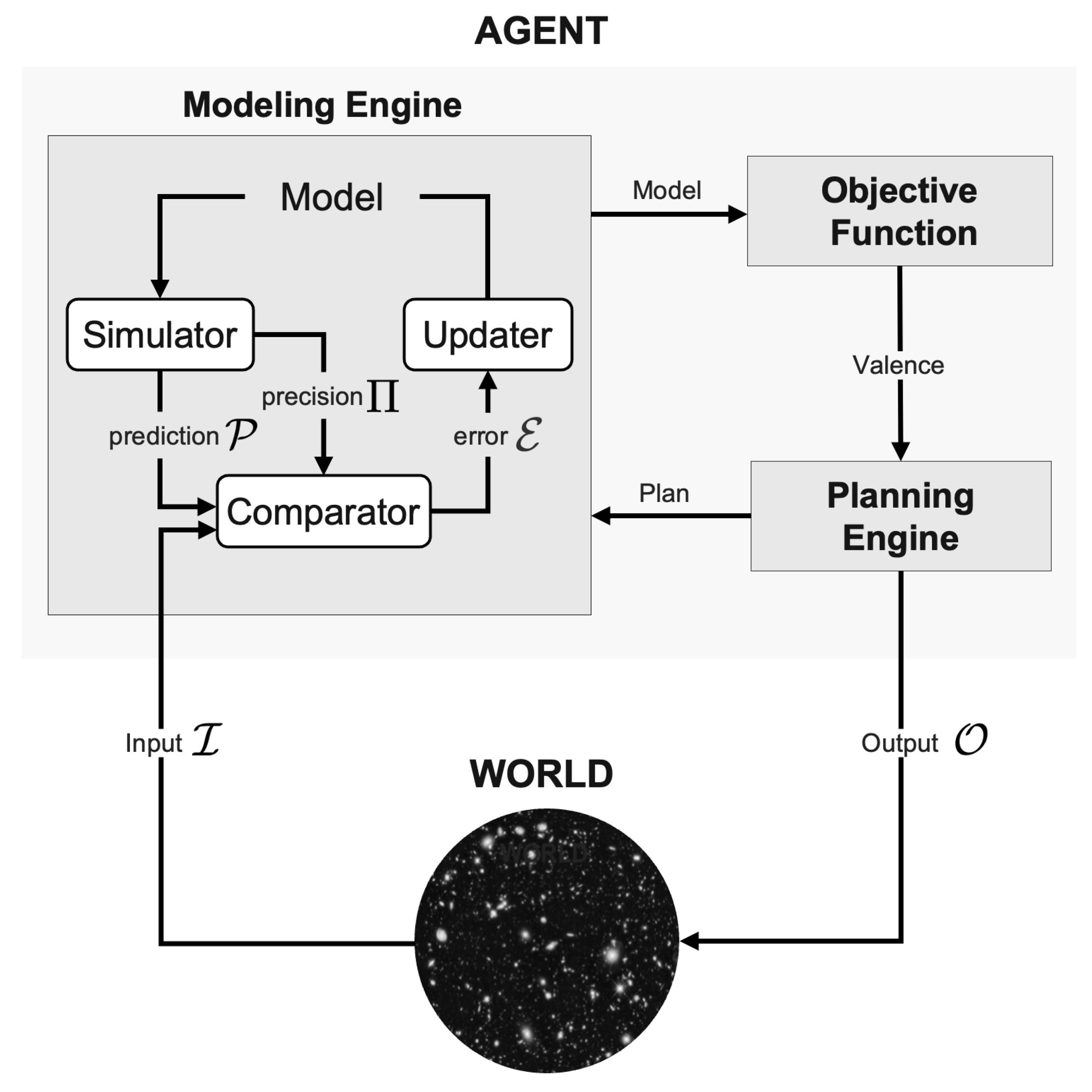
Figure 2.
The agent (robot) explores a grand library, dynamically building a world model to compress diverse and noisy data as it collects more pages.
Figure 2.
The agent (robot) explores a grand library, dynamically building a world model to compress diverse and noisy data as it collects more pages.

Figure 3.
The agent coarse-grains the world to make sense of it. When successful, this gives rise to emergent phenomena. Not all coarse-grainings are meaningful.
Figure 3.
The agent coarse-grains the world to make sense of it. When successful, this gives rise to emergent phenomena. Not all coarse-grainings are meaningful.

Disclaimer/Publisher’s Note: The statements, opinions and data contained in all publications are solely those of the individual author(s) and contributor(s) and not of MDPI and/or the editor(s). MDPI and/or the editor(s) disclaim responsibility for any injury to people or property resulting from any ideas, methods, instructions or products referred to in the content. |
© 2026 by the authors. Licensee MDPI, Basel, Switzerland. This article is an open access article distributed under the terms and conditions of the Creative Commons Attribution (CC BY) license (http://creativecommons.org/licenses/by/4.0/).
Copyright: This open access article is published under a Creative Commons CC BY 4.0 license, which permit the free download, distribution, and reuse, provided that the author and preprint are cited in any reuse.


