Preprint
Article

Preference Neural Network

Altmetrics

Downloads

983

Views

884

Comments

1

A peer-reviewed article of this preprint also exists.

Submitted:

18 April 2023

Posted:

19 April 2023

You are already at the latest version

Alerts
Abstract
Equality and incomparability multi-label ranking have not been introduced to learning before. This paper proposes new native ranker neural network to address the problem of multi-label ranking including incomparable preference orders using a new activation and error functions and new architecture. Preference Neural Network PNN solves the multi-label ranking problem, where labels may have indifference preference orders or subgroups which are equally ranked. PNN is a nondeep, multiple-value neuron, single middle layer and one or more output layers network. PNN uses a novel positive smooth staircase (PSS) or smooth staircase (SS) activation function and represents preference orders and Spearman ranking correlation as objective functions. It is introduced in two types, Type A is traditional NN architecture and Type B uses expanding architecture by introducing new type of hidden neuron has multiple activation function in middle layer and duplicated output layers to reinforce the ranking by increasing the number of weights. PNN accepts single data instance as inputs and output neurons represent the number of labels and output value represents the preference value. PNN is evaluated using a new preference mining data set that contains repeated label values which have not experimented on before. SS and PS speed-up the learning and PNN outperforms five previously proposed methods for strict label ranking in terms of accurate results with high computational efficiency.
Keywords: 
Subject: Computer Science and Mathematics  -   Artificial Intelligence and Machine Learning

1. Introduction

PREFERENCE learning (PL) is an extended paradigm in machine learning that induces predictive preference models from experimental data [1,2,3]. PL has applications in various research areas such as knowledge discovery and recommender systems [4]. Objects, instances, and label ranking are the three main categories of PL domain. Of those, label ranking (LR) is a challenging problem that has gained importance in information retrieval by search engines [5,6]. Unlike the common problems of regression and classification [7,8,9,10,11,12,13], label ranking involves predicting the relationship between multiple label orders. For a given instance x from the instance space x , there is a label L associated with x , L π , where π = { λ 1 , . . , λ n }, and n is the number of labels. LR is an extension of multi-class and multi-label classification, where each instance x is assigned an ordering of all the class labels in the set L. This ordering gives the ranking of the labels for the given x object. This ordering can be represented by a permutation set π = { 1 , 2 , , n } . The label order has the following three features. irreflexive where λ a λ a ,transitive where ( λ a λ b ) ( λ b λ c ) λ a λ c and asymmetric λ a λ b λ b λ a . Label preference takes one of two forms, strict and non-strict order. The strict label order ( λ a λ b λ c λ d ) can be represented as π = ( 1 , 2 , 3 , 4 ) and for non-restricted total order π = ( λ a λ b λ c λ d ) can be represented as π = ( 1 , 2 , 2 , 3 ) , where a , b , c , a n d , d are the label indexes and λ a , λ b , λ c and λ d are the ranking values of these labels.
For the non-continuous permutation space, The order is represented by the relations mentioned earlier and the incomparability binary relation. For example the partial order λ a λ b λ d can be represented as π = ( 1 , 2 , 0 , 3 ) where 0 represents an incomparable relation since λ c is not comparable to ( λ a , λ b , λ d ).
Various label ranking methods have been introduced in recent years [14], such as decomposition-based methods, statistical methods, similarity, and ensemble-based methods. Decomposition methods include pairwise comparison [15,16], log-linear models and constraint classification [17]. The pairwise approach introduced by Hüllermeier [18] divides the label ranking problem into several binary classification problems to predict the pairs of labels λ i λ j or λ j λ i for an input x. Statistical methods includes decision trees [19], instance-based methods (Plackett-Luce) [20] and Gaussian mixture model based approaches. For example, Mihajlo uses Gaussian mixture models to learn soft pairwise label preferences [21].
The artificial neural network (ANN) for ranking was first introduced as (RankNet) by Burge to solve the problem of object ranking for sorting web documents by a search engine [22]. Rank net uses gradient descent and probabilistic ranking cost function for each object pair. The multilayer perceptron for label ranking (MLP-LR) [23] employs a network architecture using a sigmoid activation function to calculate the error between the actual and expected values of the output labels. However, It uses a local approach to minimize the individual error per output neuron by subtracting the actual-predicted value and using Kendall error as a global approach. Neither direction uses a ranking objective function in backpropagation (BP) or learning steps.
The deep neural network (DNN) is introduced for object ranking to solve document retrieval problems. RankNet [22], RankBoost [24], and Lambda MART [25], and deep pairwise label ranking models  [26], are convolution neural Network (CNN) approaches for the vector representation of the query and document-based. CNN is used for image retrieval [27] and label classification for remote sensing and medical diagnosing [28,29,30,31,32,33,34,35]. A multi-valued activation function has been proposed by Moraga and Heider [36] to propose a Generalized Multiple–valued Neuron with a differentiable soft staircase activation function, which is represented by a sum of a set of sigmoidal functions. In addition, Aizenberg proposed a generalized multiple-valued neuron using a convex shape to support complex numbers neural network and multi-values numbers [37]. Visual saliency detection using the Markov chain model is one approach that simulates the human visual system by highlighting the most important area in an image and calculating superpixels as absorbing nodes [38,39,40]. However, this approach needs a saliency optimization on the results and has calculation cost [41,42].
Particle Swarm Optimization in movement detection is based on the concept of variation and inter-frame difference for feature selection. The swarm algorithms are mainly used in human motion detection in sports, and it is used based on probabilistic optimization algorithm [43,44,45,46] and CNN [47].
Some of the methods mentioned above and their variants have some issues that can be broadly categorized into three types:
1)
The ANN Predictive probability can be enhanced by limiting the output ranking values in the SS functions to a discrete value instead of a range of values of the rectified linear unit (Relu), Sigmoid, or Softmax activation functions. The predictive is enhanced by using the SS function slope as a step function to create discrete values, accelerating the learning by reducing the output values to accelerate the ranking convergence.
2)
The drawback of ranking based on the classification technique ignores the relation between multiple labels: When the ranking model is constructed using binary classification models, these methods cannot consider the relationship between labels because the activation functions do not provide deterministic multiple values. Such ranking based on minimizing pairwise classification errors differs from maximizing the label ranking’s performance considering all labels. This is because pairs have multiple models that may reduce ranking unification by increasing ranking pairs conflicts where there is no ground truth, which has no generalized model to rank all the labels simultaneously. For example, D = ( 1 , 1 , 1 ) for π = ( λ a λ b λ c ) and D = ( 1 , 1 , 1 ) for π = ( λ a λ c λ b ) the ranking is unique; however, pairwise classification creates no ground truth ranking for the pair λ b λ c and λ c λ b which adds more complexity to the learning process.
3)
Ignoring the relation between features. The convolution kernel has a fixed size that detects one feature per kernel. Thus, it ignores the relationship between different parts of the image. For example, CNN detects the face by combining features (the mouth, two eyes, the face oval, and a nose) with a high probability of classifying the subject without learning the relationship between these features. For example, the proposed PN kernel start attention to the important features that have a high number of pixel ranking variation.
The main contribution of the proposed neural network is
  • Solving the label ranking as a machine learning problem.
  • Solving the deep learning classification problem by employing computational ranking in feature selection and learning.
Where PNN has several advantages over existing label ranking methods and CNN classification approaches.
1)
PNN uses the smooth staircase SS as an activation function that enhances the predictive probability over the sigmoid and Softmax due to the step shape that enhances the predictive probability from a range from -1 to 1 in the sigmoid to almost discrete multi-values.
2)
PNN uses gradient ascent to maximize the spearman ranking correlation coefficient. In contrast, other classification-based methods such as MLP-LR use the absolute difference of root mean square error (RMS) by calculating the differences between actual and predicted ranking and other RMS optimization, which may not give the best ranking results.
3)
PNN is implemented directly as a label ranker. It uses staircase activation functions to rank all the labels together in one model. The SS or PSS functions provide multiple output values during the conversions; however, MLP-LR and RankNet use sigmoid and Relu activation functions. These activation functions have a binary output. Thus, it ranks all the labels together in one model instead of pairwise ranking by classification.
4)
PN uses a novel approach for learning the feature selection by ranking the pixels and using different sizes of weighted kernels to scan the image and generate the features map.
The next section explains the Ranker network experiment, problem formulation, and the PNN components (Activation functions, Objective function, and network structure) that solve the Ranker problems and comparison between Ranker network and PNN.

2. PNN Components

2.1. Initial Ranker

The proposed PNN is based on an initial experiment to implement a computationally efficient label ranker network based on the Kendall τ error function and sigmoid activation function using simple structure as illustrated in Section 4 Figure 6.
The ranker network is a fully connected, three-layer net. The input represents one instance of data with three inputs, and there are six neurons in the hidden layer and three output neurons representing the labels’ index. Each neuron represents the ranking value. A small toy data set is used in this experiment. The ranker uses RMS gradient descent as an error function to measure the difference between the predicted and actual ranking values. The ranker has Kendall τ as a stopping criterion. The same ANN structure, number of neurons and learning rate using SS activation function, and spearman error function and gradient ascent of ρ will be discussed in Section IV. The ranking convergence reaches τ 1 after 160 epochs using the Sigmoid function [48]. The sigmoid and ReLU shapes have a slightly high rate of change of y, and it produces a larger output range of data. Therefore, we consider ranking performance as one of the disadvantages of sigmoid function in the ranker network.
The ranker network has two main problems.
1)
The ranker uses two different error functions, RMS for learning and Kendall τ for stopping criteria. Kendall τ is not used for learning because it is not continuous or differentiable. Both functions are not consistent as stopping criteria measure the relative ranking, and RMS does not, which may lead to incorrect stopping criteria. Enhancing the RMS may not also increase the error performance, as illustrated in Figure 3 in a comparison between the ranker network. evaluation using ρ and RMS.
2)
The convergence performance takes many iterations to reach the ranking τ 1 based on the shape of sigmoid or Relu functions and learning rate as shown in the experiment video link [48] due to the slope shape between -1 or 0 and 1. The prediction probability almost equals the values from -1 or 0 to 1.

2.2. Problem Formulation

For multi-class and multi-label problems, learning the data’s preference relation predicts the class classification and label ranking. i.e., data instance D { x 1 , x 2 , , x n } . the output labels are predicted as ranked set labels that have preference relations L = { λ y 1 , , λ y n } . PNN creates a model that learns from an input set of ranked data to predict a set of new ranked data. The next section presents the initial experiment to rank labels using the usual network structure.

2.3. Activation Functions

The usual ANN activation functions have a binary output or range of values based on a threshold. However, these functions do not produce multiple deterministic values on the y-axis. This paper proposes new functions to slow the differential rate around ranking values on the y-axis to solve ranking instability. The proposed functions are designed to be non-linear, monotonic, continuous, and differentiable using a polynomial of the tanh function. The step width maintains the stability of the ranking during the forward and backward processes. Moraga [36] introduced a similar multi-valued function. However, the proposed exponential derivative was not applied to an ANN implementation. Moraga exponential function is geometrically similar to the step function [49]. However, The newly proposed functions consist of tanh polynomial instead of exponential due to the difficulty in implementation. The new functions detect consecutive integer values, and the transition from low to high rank (or vice versa) is fast and does not interfere with threshold detection.

2.3.1. Positive Smooth Staircase (PSS)

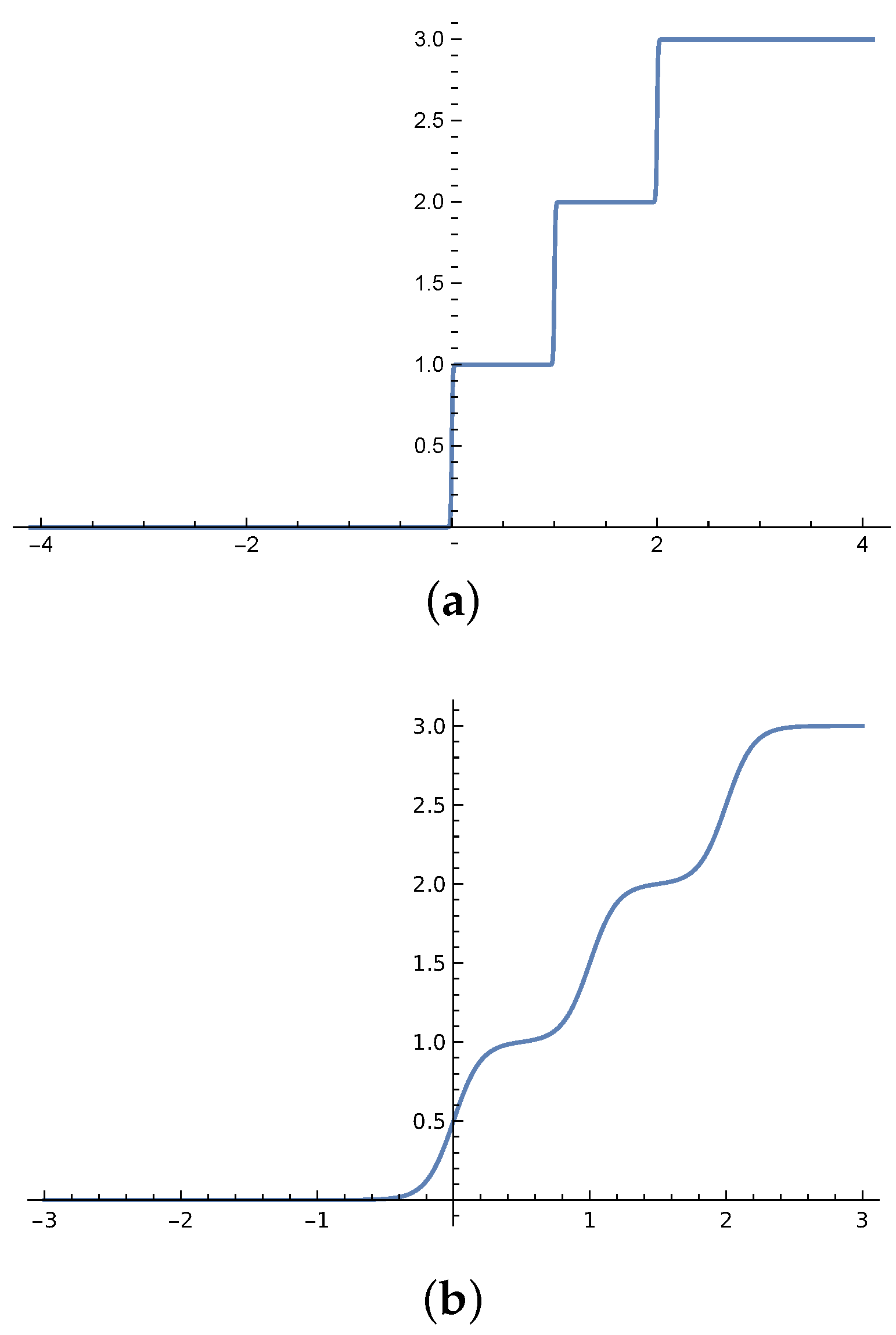
As a non-linear and monotonic activation function, a positive smooth staircase (PSS) is represented as a bounded smooth staircase function starting from x=0 to . Thus, it is not geometrically symmetrical around the y-axis as shown in Figure 1. PSS is a polynomial of multiple tanh functions and is therefore differentiable and continuous. The function squashes the output neurons values during the FF into finite multiple integer values. These values represent the preference values from {0 to n} where 0 represents the incomparable relation and values from 1 to n represent the label ranking. The activation function is given in Equation (1). PSS is scaled by increasing the step width w
y = 1 2 s ( i = 0 n 1 tanh c ( w i x ) n )
Where n is the number of stair steps equal to the number of labels to rank, w is the step width, and c is the stair curvature c = 100 and 5 for the sharp and smooth step, respectively. and s is the scaling factor for reducing the height of each step to range to rank value with decimal place for the regression problems. s=10 and s=100 for 1 and 2 decimal places, respectively, s is calculated as in Equation (2).
n = Y m a x s
and w is the step width as shown in Equation (3).
2 b = w ( n 1 )

2.3.2. Smooth Staircase (SS)

The proposed (SS) represents a staircase similar to (PSS). However, SS has a variable boundary value used as a hyperparameter in the learning process. The derivative of the activation function is discussed in Section 3 and the performance comparison between SS and PSS is mentioned in Section 5.
The activation function is given in Equation (4).
y = 1 2 s ( i = 0 n 1 tanh c ( b x w i ) n )
where c is step curvature, n = number of ranked labels, b is the boundary value on the x-axis, and (SS) lies between b and b.
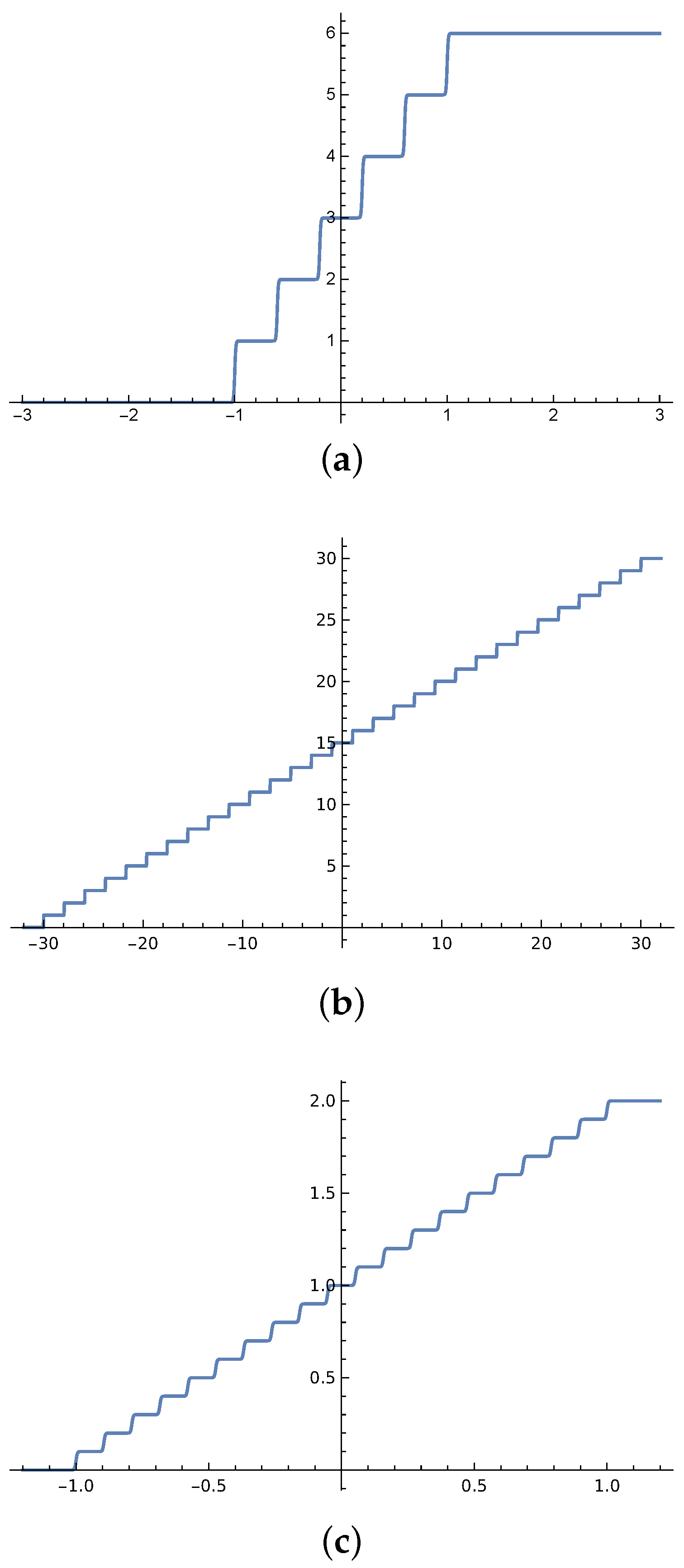
Where Y m a x is the max. value to rank. i.e., Y m a x =3 and values have one decimal place. n =30 The (SS) function has the shape of smooth stair steps, where each step represents an integer number of label ranking on the y-axis from 0 to as shown in Figure 1, The SS step is not flat, but it has a differential slope. The function boundary value on the x-axis is from -b to b Therefore, input values must be scaled from -b to b. The step width is 1 when n 2 b . The convergence rate is based on the step width. However, it may take less time to converge based on network hyper parameters. Figure 2a,b. The SS is scaled by increasing the boundary value b

2.4. Ranking Loss Function

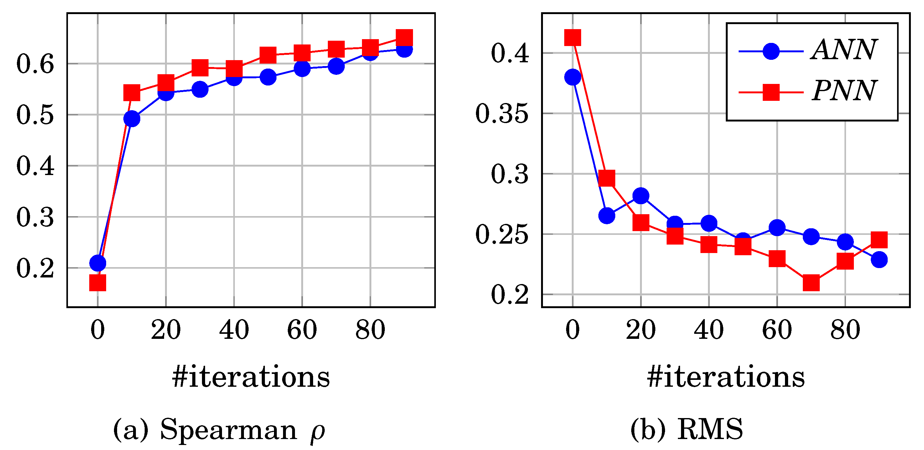
Two main error functions have been used for label ranking; Kendall τ  [50] and spearman ρ  [51]. However, the Kendall τ function lacks continuity and differentiability. Therefore, the spearman ρ correlation coefficient is used to measure the ranking between output labels. spearman ρ error derivative is used as a gradient ascent process for BP, and correlation is used as a ranking evaluation function for convergence stopping criteria. τ A v g is the average τ per label divided by the number of instances m, as shown in line 8 of Algorithm 1. spearman ρ measures the relative ranking correlation between actual and expected values instead of using the absolute difference of root means square error (RMS) because gradient descent of RMS may not reduce the ranking error. For example, π 1 = ( 1 , 2.1 , 2.2 ) and π 2 = ( 1 , 2.2 , 2.1 ) , have a low RMS = 0.081 but a low ranking correlation ρ = 0.5 and τ = 0.3 .
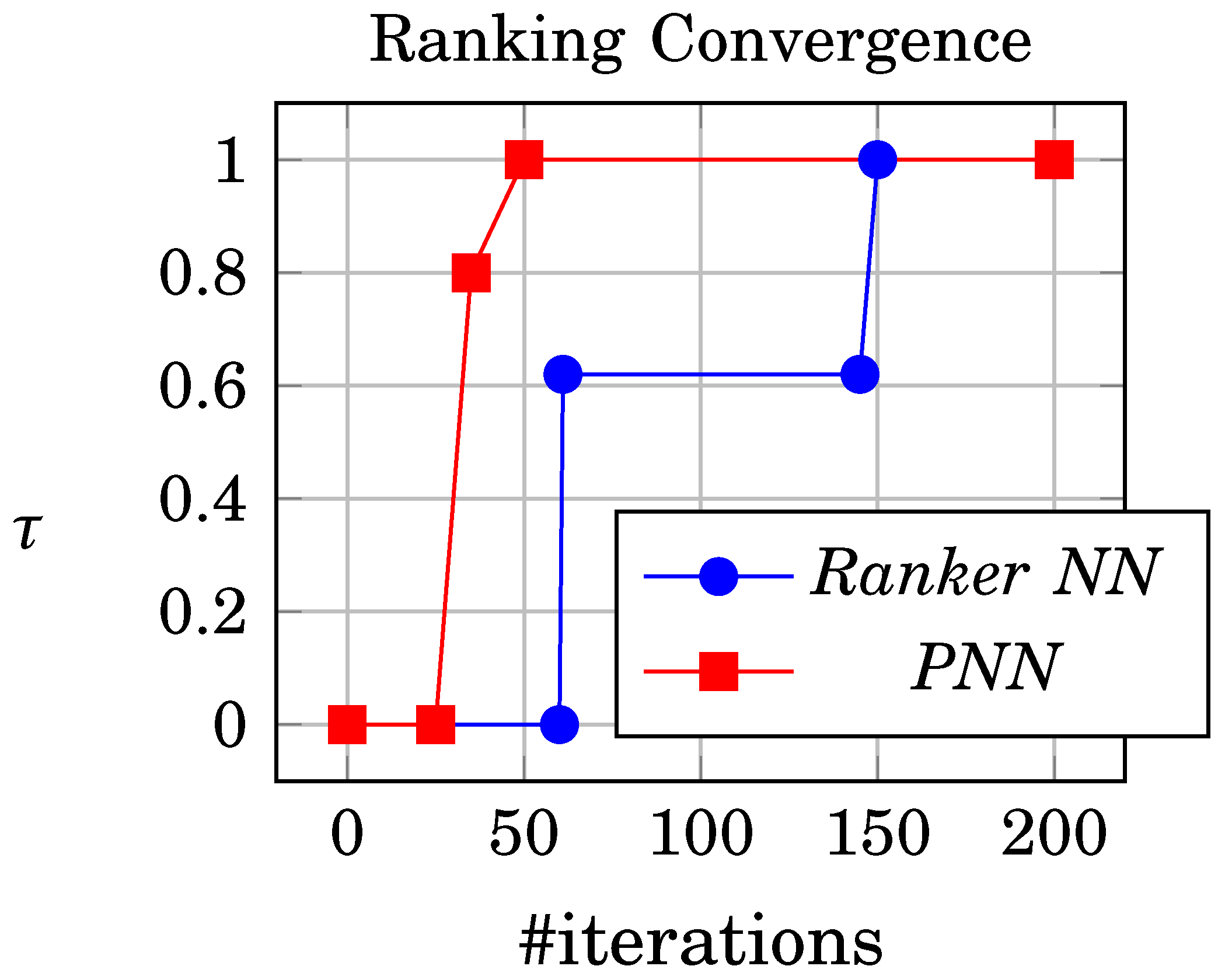
Figure 3 shows the comparison between the initial ranker network and PNN; the ranker network uses Kendall τ which has lower performance as a stopping criterion compared to PNN spearman because the stopping criteria are based on the RMS per iteration; however, PNN uses spearman for both ranking step and stopping criteria.
Figure 3. Ranker network and PNN evaluation in terms of RMS and spearman correlation error functions.
Preprints 71295 g003
The spearman error function is represented by Equation (5)
ρ = 1 6 i = 1 m ( y i y t i ) 2 m ( m 2 1 )
where y i , y t i , i and m represent rank output value, expected rank value, label index and number of instances, respectively.

2.5. PNN Structure

2.5.1. One Middle Layer

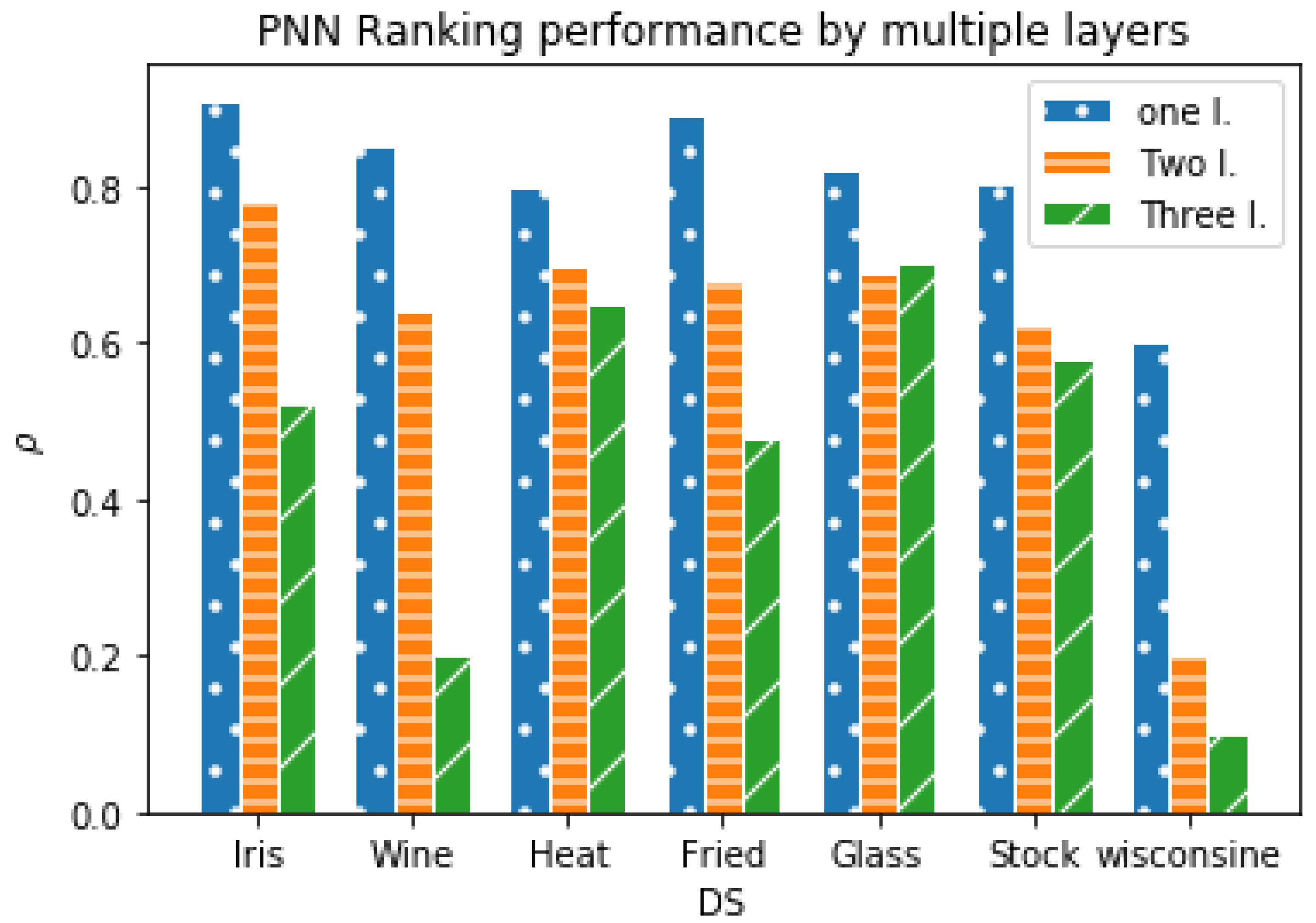
The ANN has multiple hidden layers. However, we propose PNN with a single middle layer instead of multi-hidden layers because ranking performance is not enhanced by increasing the number of hidden layers due to fixed multi-valued neuron output, as shown in Figure 4; Seven benchmark data sets  [52] was experimented using SS function using one, two, and three hidden layers with the following hyper parameters; learning rate (l.r.)=0.05, and each layer has neuron i = 100 and b = 10 ). We found that by increasing the number of hidden layers, the ranking performance decreases, and more iterations are required to reach ρ 1 . The low performance because of the shape of SS produces multiple deterministic values, which decrease the arbitrarily complex decision regions and degrees of freedom per extra hidden layer.

2.5.2. Preference Neuron

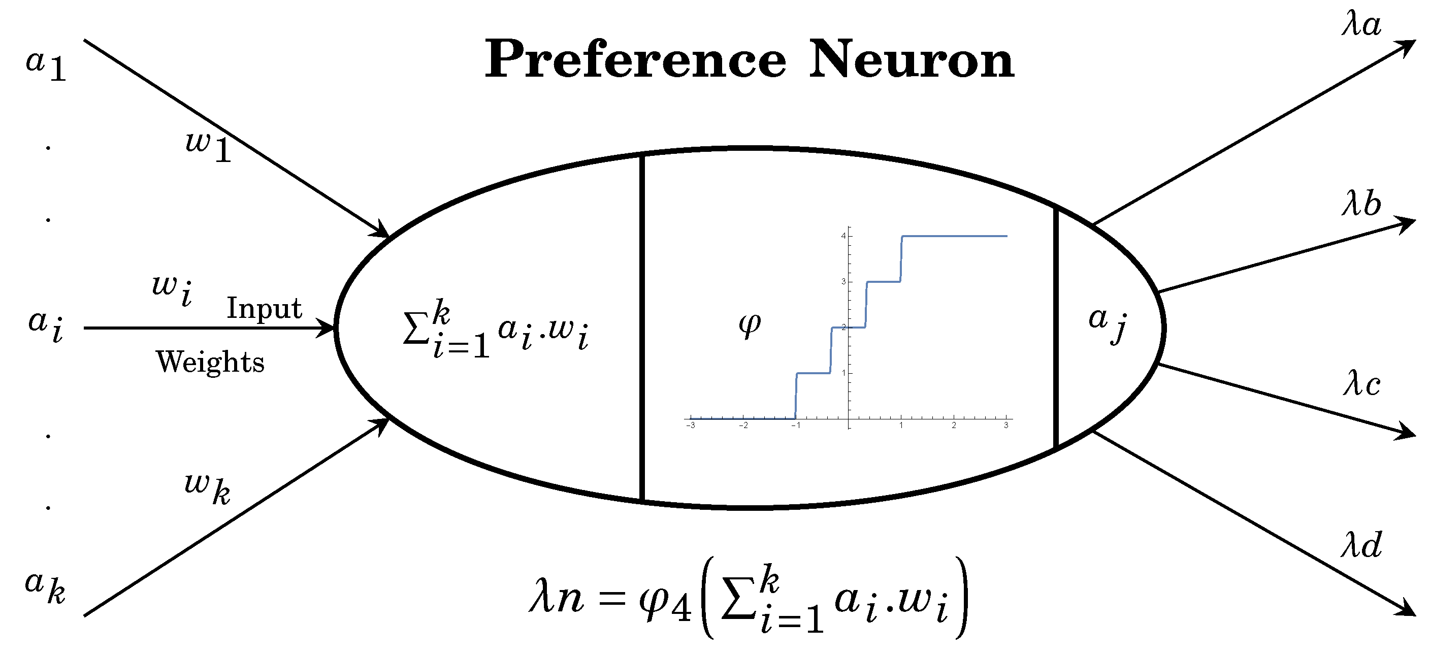
Preference Neuron are a multi-valued neurons uses a PSS or SS as an activation function. Each function has a single output; however, PN output is graphically drawn by n number of arrow links that represent the multi-deterministic values. The PN in the middle layer connects to only n output neurons s t p = n + 1 ; where s t p is the number of SS steps. The PN in the output layer represents the preference value. The middle and output PNs produce a preference value from 0 to as illustrated in Figure 5.
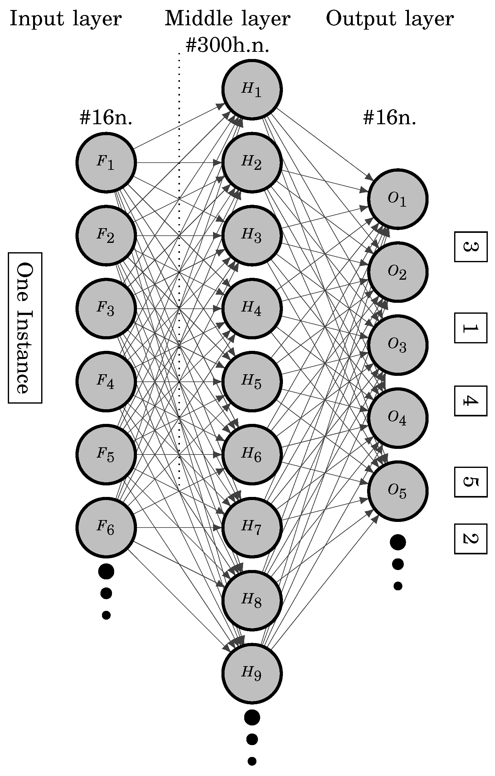
The PNN is fully connected to multiple-valued neurons and a single-hidden layer ANN. The input layer represents the number of features per data instance. The hidden neurons are equal to or greater than the number of output neurons, H n L n , to reach error convergence after a finite number of iterations. The output layer represents the label indexes as neurons, where the labels are displayed in a fixed order, as shown in Figure 6.
Figure 6. PNN where φ n = 16 , f i n = 16 and λ o u t = 16 , per x 1 , π 1 , L { λ a , λ b , λ c , λ d } where π 1 = { 1 , 2 , 3 , 4 , , 16 } .
Preprints 71295 g006
The ANN is scaled up by increasing the hidden layers and neurons; however, increasing the hidden layers in PNN does not enhance the ranking correlation because it does not arbitrarily increase complex decision regions and degrees of freedom to solve more complex ranking problems. This limitation is due to the multi-semi discrete-valued activation function, limiting the output data variation. Therefore, instead of increasing the hidden layer, PNN is scaling up by increasing the number of neurons in the middle layer and scaling input data boundary value and increasing the PSS step width and SS boundaries which are equal to the input data scaling value, which leads to increased data separability.
PNN reaches ranking ρ 1 after 24 epochs compared to the initial ranker network that reaches the same result in 200 iterations, The video link demonstrates the ranking convergence as shown in Figure 7 and video [48]. A summary of the three networks is presented in Table 1.
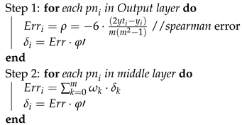
The output labels represent the ranking values. The differential PSS and SS functions to accelerate the convergence after a few iterations due to the staircase shape, which achieves stability in learning. PNN simplifies the calculation of FF and BP, and updates weights into two steps due to single middle layer architecture. Therefore, the batch weight updating technique is not used in PNN, and pattern update is used in one step. The network bias is low due to the limited preference neuron output of data variance; thus it is not calculated. Each neuron uses the SS or PS activation function in FF step, and calculates the preference number from 1 to n, where n is the number of label classes. During BP. The processes of FF and BP are executed in two steps until ρ A v g 1 or the number of iterations reaches ( 10 6 ) as mentioned in the algorithm section.
The SS step width decreases by increasing the number of labels; thus, we increase function boundary b to increase the step width to 1 to make the ranking convergence; In addition, a few complex data sets may need more data separability to enhance the ranking. Therefore, we use the b value as a hyperparameter to keep the stair width > = 1 and normalize input data from b to b.
Table 1 shows a brief comparison between Ranker ANN and PNN.
The following section describes the data preprocessing steps, feature selections, and components of PN.

3. PN Components

3.1. Image Preprocessing

3.1.1. Greyscale Conversion

Data scaling as red, green, and blue (RGB) colors is not considered for ranking because PN measures the preference values between pixels. Thus, The image is converted from RGB color to Greyscale.

3.1.2. Pixels’ Sorting

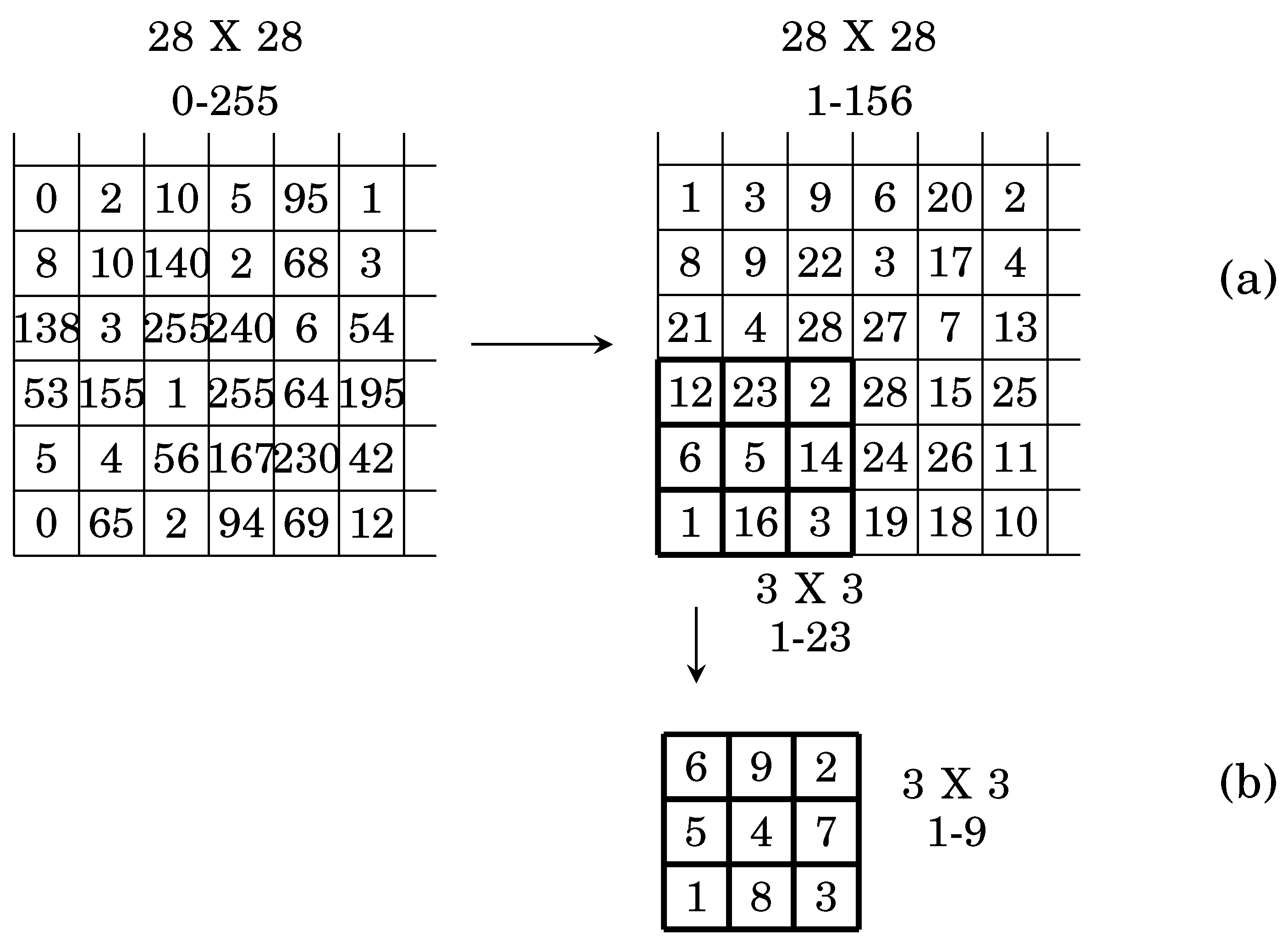
Ranking the image from π = { λ 1 , . . , λ m } to π = { λ 1 , . . , λ k } where the maximum greyscale value λ m = 255 and λ k is the maximum ranked pixel value as illustrated in Figure 8a.

3.1.3. Pixels Averaging

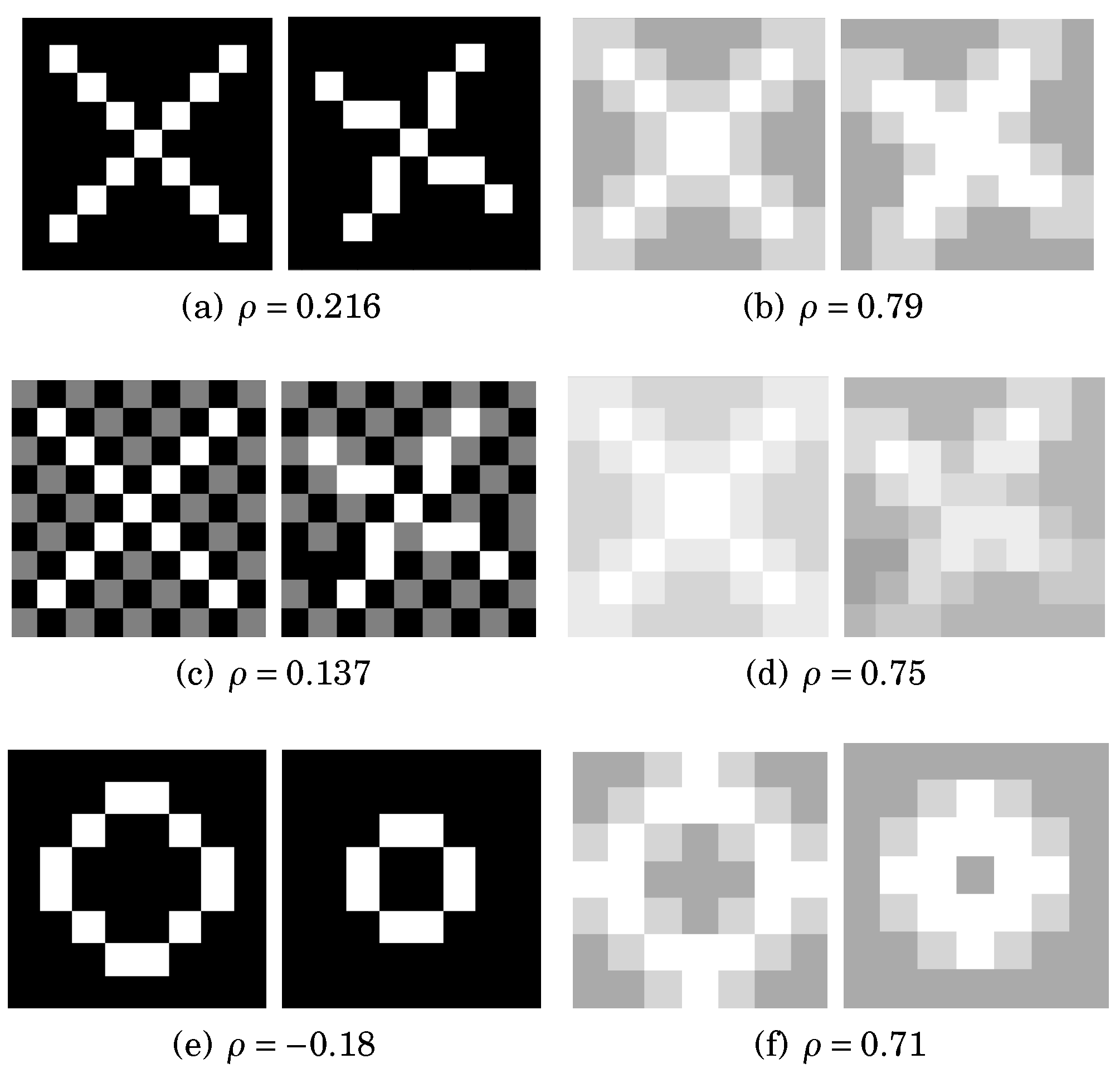
Ranking image pixels has an almost low ranking correlation due to noise, scaling, light, and object movement; therefore, window averaging is proposed by calculating the mean of pixel values of the small flattened window size of 2x2 of 4 pixels as shown in Figure 9. The overall image ρ of pixels increased from 0.2 to 0.79 in (a and b), from 0.137 to 0.75 for noisy images in (s and d), and scaled images from -0.18 to 0.71 in (e and f).
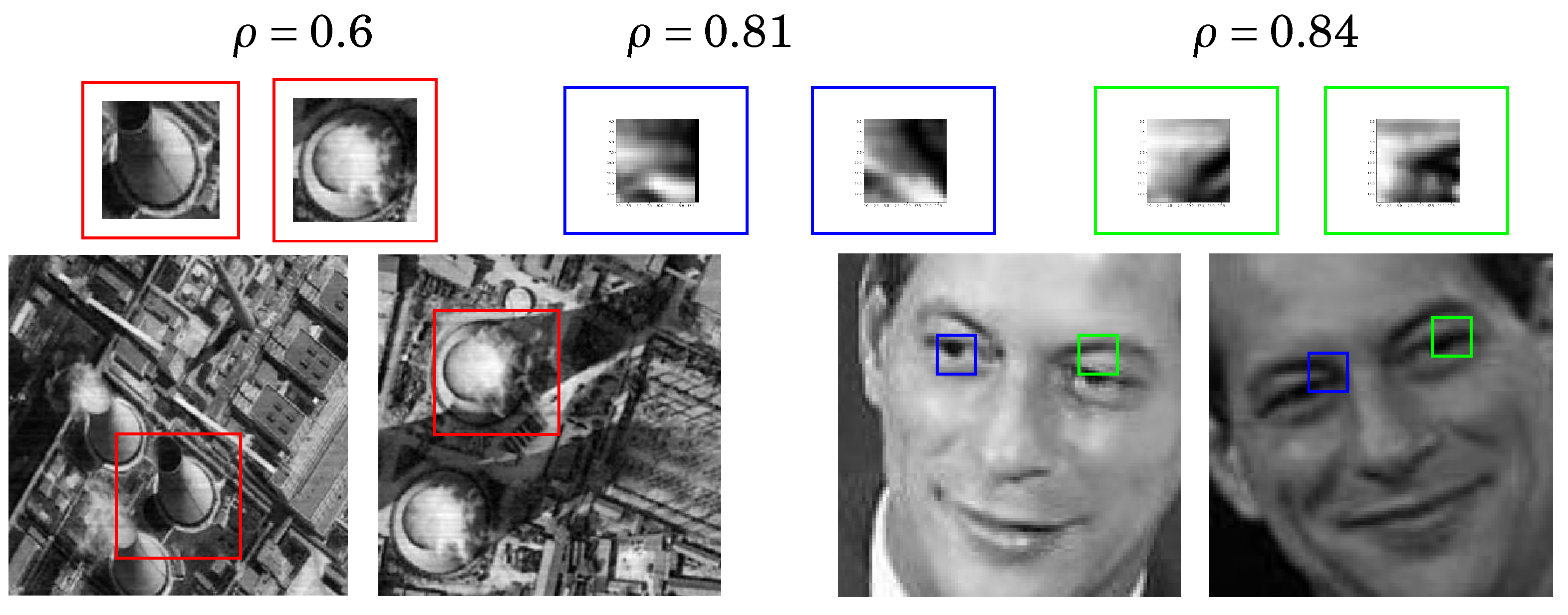
The two approaches, Pixel ranking and Averaging has been tested in remote sensing and faces images to detect the similarity, and it shows high ranking correlations using different window size as shown in Figure 10. It detects the high correlation by starting from the large window size = image size. It reduces the size and scans until it reaches the highest correlation.

3.2. Feature Selection By Attention

Feature selection for the kernel proceeded by selecting the features with a high group of pixel ranking variations indicating the importance of the scanned kernel area. This kind of hard attention makes the selection based on the threshold of pixel ranking values. to reduce the dimension of the input image.

3.3. Feature Extraction

This paper proposes a new approach for image feature selection based on the preference values between pixels instead of the convolution of pixels array as implemented in CNN. The PN’s features are based on ranking computational space. Therefore, the kernel window size is considered a factor for feature selection.

3.3.1. Pixels Resorting

The flattened window’s values are sorted for each kernel window in the image. The Figure 8b shows the window size 3X3 range from λ k 1 = 23 to λ k 2 = 9 . Pixel sorting reduces the data margin, Thus, it reduces the computational complexity.

3.3.2. Weighted Ranker Kernel

The kernel weights are randomly initialized from -0.05 to 0.05. The kernel learns the features by BP of its weights to select the best feature. the partial change in the kernel is calculated by differentiating the spearman correlation as in Equation (6)
d K w = 2 · I m g w d ρ · n 3 n 6
Different kernel sizes could be used for big images’ size. We use three different kernels to capture the relations between different features.

3.3.3. Max Pooling

Max. pooling is used to reduce the features map’s size and select the highest correlation values to feed to the PNN.

3.4. PN Structure

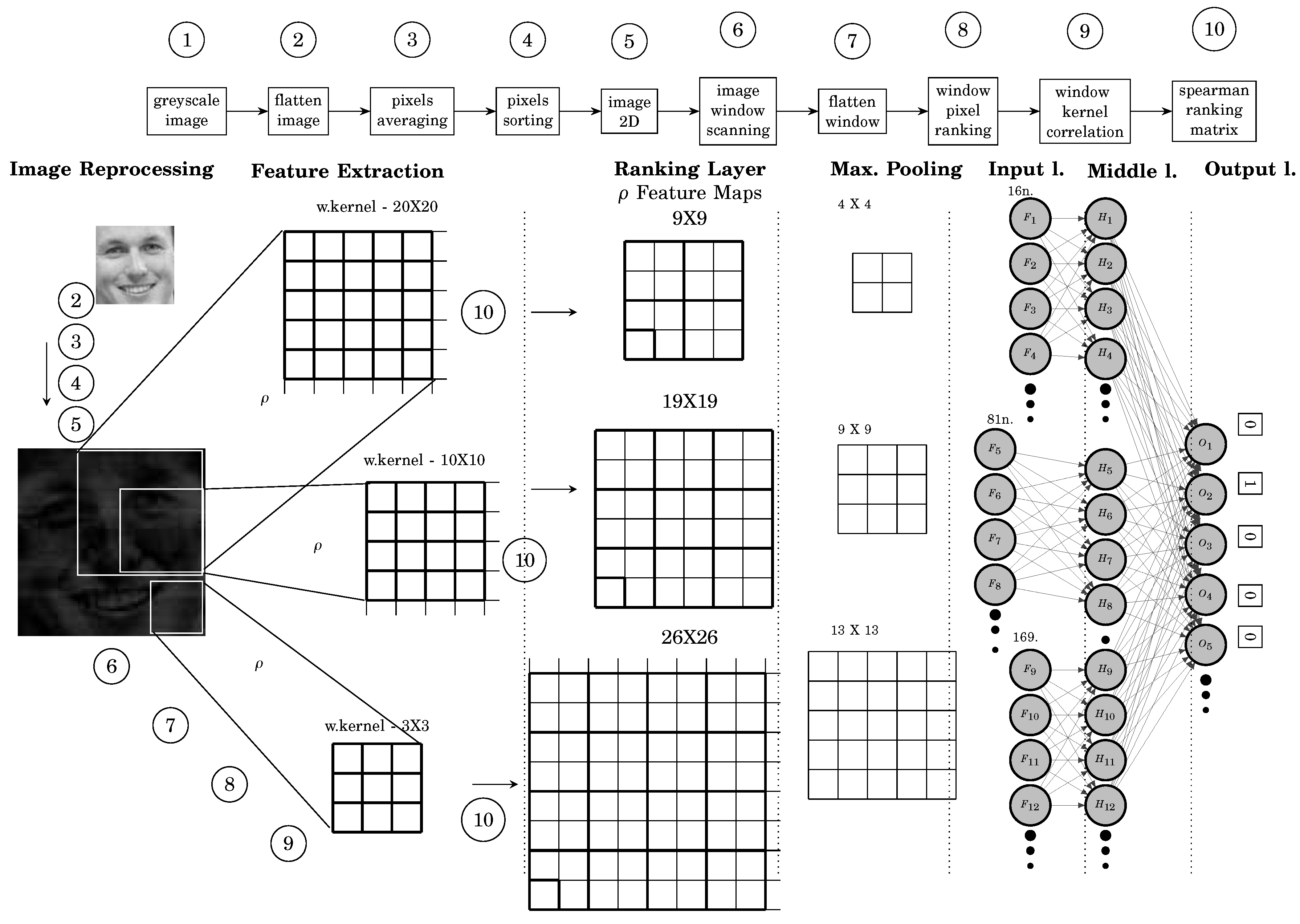
PN is the deep learning structure of PNN for image classification. It consists of five layers, a ranking features map and a max. pooling and three PNN layers. PN has one or multiple different sizes of PNNs connected by one output layer. Each PNN has SS or PSS where φ n = 2 for binary ranking to map the classification. The number of output neurons is the number of classes. The structure is shown in Figure 11. PN have one or more ranker kernels with different sizes, Each kernel has one corresponding PNN. PN uses the weighted kernel ranking to scan the image and extract the features map of spearman correlation values of the kernel with the scanned ranked image window as ρ ( π k , π w ) where π k is the kernel preference values and π w is the scanned window image preference values. Each kernel scans the image by one step and creates a spearman features list. Max. Pooling is used to minimize the feature map used as input to PNN.
One 5X5 kernel is used for fashion Mnist data set [53]. Three kernels with sizes (3, 10, and 20) are used for CFAR-100 [54].

3.5. Choosing The Kernel Size

Kernel size is chosen based on the hard attention of the highest group of pixels that has high ranking variation. The process scans the image sequentially starting from a small size to find the size with the highest pixels ranking variation. For example for the Mnist dataset where the image has a size of 28X28, The meaningful features are extracted using kernel sizes 10x10, 15x15, 20x20 and 25x25.

4. Algorithms

4.1. Baseline Algorithm

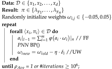
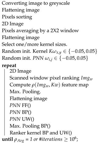
Algorithm 1 represents the three functions of the network learning process; feed-forward (FF), BP, and updating weights (UW). Algorithm 2 represents the learning flow of PN. Algorithm 3 represents the simplified BP function in two steps.    
Algorithm 1:PNN learning flow.
Preprints 71295 i001
Algorithm 2:PN Learning flow.
Preprints 71295 i002
Algorithm 3:PNN BP.
Preprints 71295 i003

4.2. Ranking Visualization

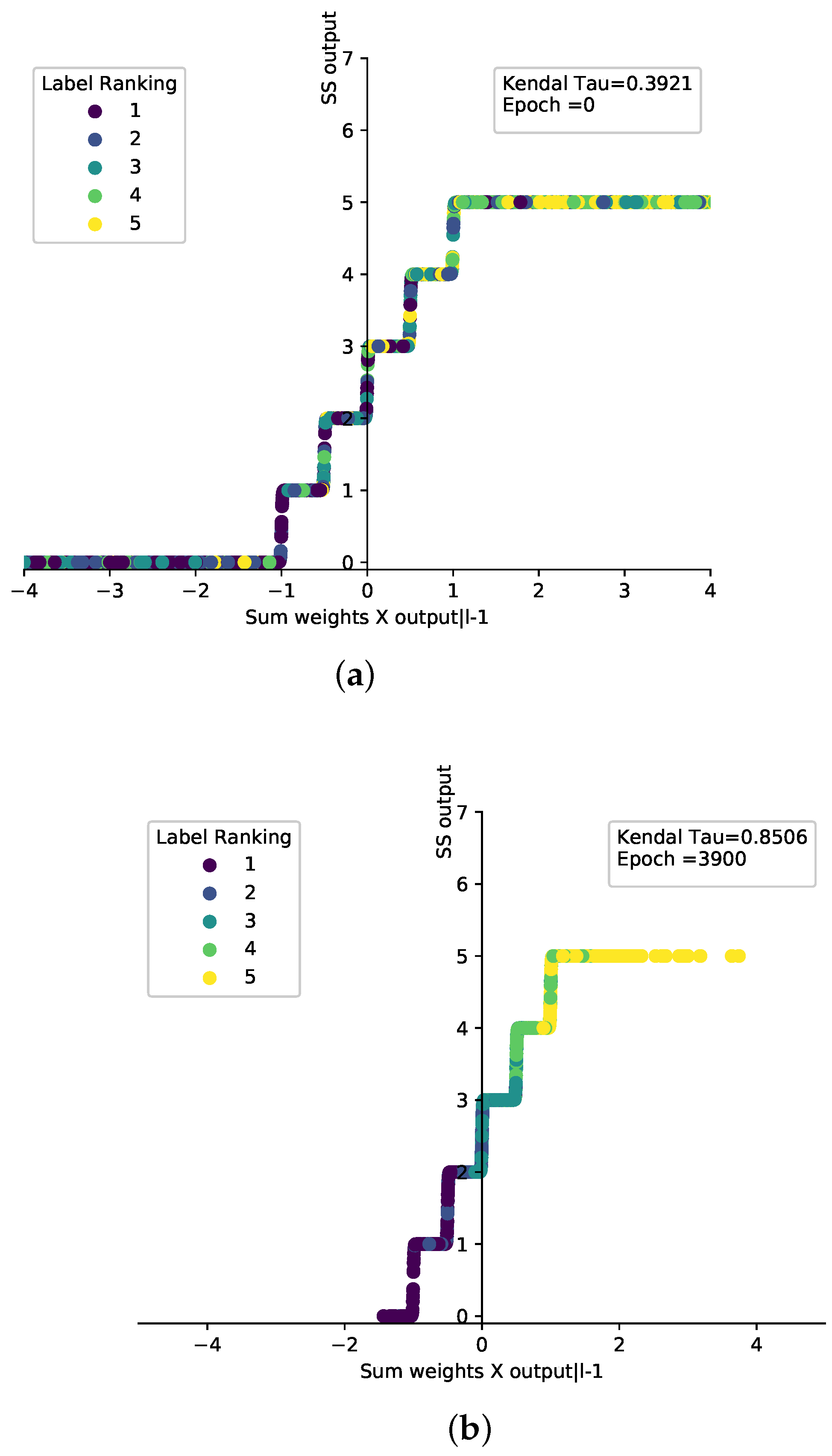
PNN ranking convergence is visualized using the SS function by displaying the normalized input data points with corresponding actual ranked five labels represented in 5 different colours, The plotting of input value and SS output values per iteration is shown in Figure 12, which illustrates the distribution of SS output values against the actual colour values at iterations 0 and 3900 and τ is enhanced from 0.39 to 0.85.

4.3. Complexity Analysis

4.3.1. Time Complexity

  • FF time complexity corresponds to FF of middle and output layers, and m and n are the number of nodes in the middle and output layers. W m and W o are weighted matrix and S S t is the activation function of number of instances t. The time complexity in Equation (7)
    O ( m · o · t )
  • BB starts with calculating the error of output layer E o t = ρ o   D e l t a o = E o t · S S and D e l t a m = E m t · S S then UW
    W m = W m D e l t a m
    This time complexity is then multiplied by the number of epochs p
    O ( p · m · o · t )

4.3.2. Input Neurons

The number of PN input neurons is represented by Equation (10)
# I n p u t = ( I m g w K w + 1 ) · ( I m g h K h + 1 )
where w and h are width and height of kernel and image.

5. Network Evaluation

This section evaluates the PNN against different activation functions and architectures. All weights are initialized = 0 to compare activation functions and A and B have the same initialized random weights to evaluate the structure.

5.1. Activation Functions Evaluation

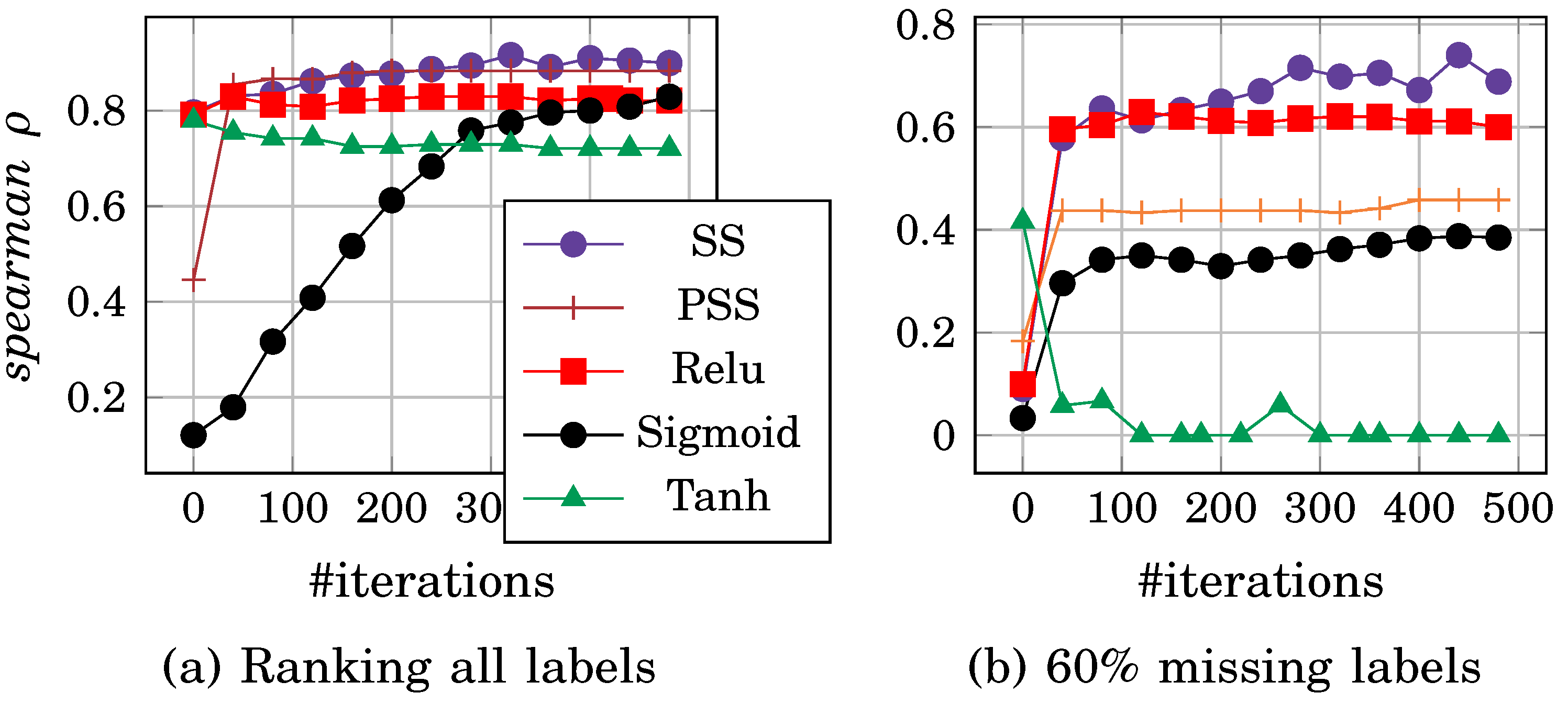
PNN is tested on iris and stock data sets using four activation functions. SS, PSS, ReLU, sigmoid, and tanh. PNN has one middle layer and the number of hidden neurons (h.n.) is 50, while l.r.= 0.05. Figure 13 shows the convergence after 500 iterations using four activation functions (SS, PSS, sigmoid, ReLU and tanh) respectively. We noticed that PSS and SS have a stable rate of ranking convergence compared to sigmoid, tanh, and ReLU. This stability is due to the stairstep width, which leads each point to reach the correct ranking during FF and BP in fewer epochs.

5.1.1. PSS and SS Evaluation

As shown in Figure 13, PSS reaches convergence and remains stable for a long number of iterations compared to SS. However, SS has better ρ than PSS. This good performance of SS is due to the reason:
  • The symmetry of SS function on the x axis. The SS shape handles both positive and negative normalized data. It reduces the number of iterations to reach the correct ranking values.
To have the same performance for SS and PSS, the input data should be scaled from 0 to step width X #steps and from -b to b for PSS and SS respectively.

5.1.2. Missing Labels Evaluation

Activation functions are evaluated by removing a random number of labels per instance. PNN marked the missing label as -1; PNN neglects error calculation during BP, δ = 0 . Thus, the missing label weights remain constants per learning iteration. The missing label approach is applied to the data set by 20% and 60% of the training data. The ranking performance decreases when the number of missing labels increases. However, SS and PSS have more stable convergence than other functions. This evaluation is performed on the iris data set, as shown in Figure 13.

5.1.3. Statistical Test

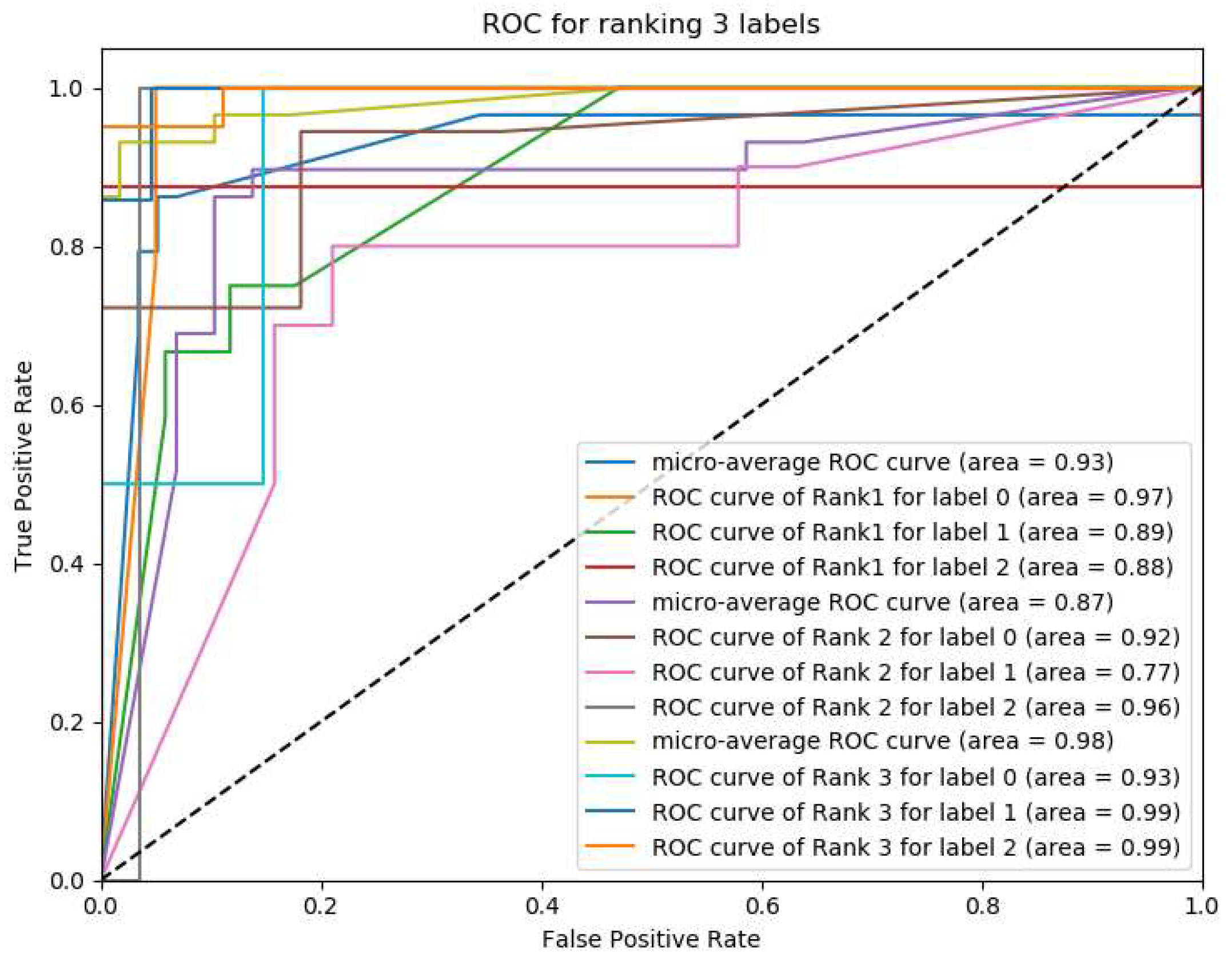
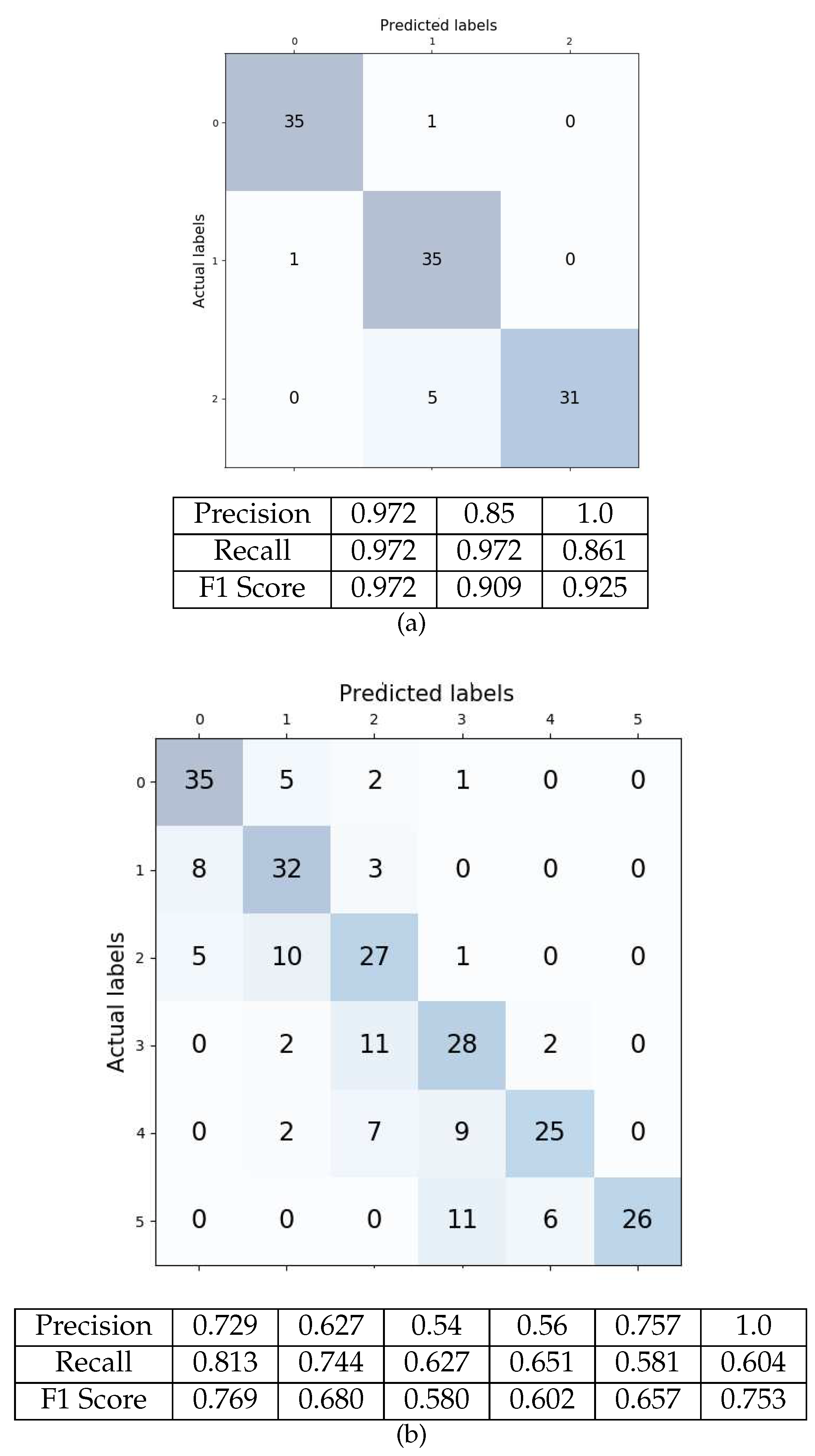
The PNN results were evaluated using receiver operating characteristic (ROC) curves. The true positive and negative for each rank are evaluated per label of wine dataset as shown in Figure 14. The confusion matrix on wine and glass DS are shown in Figure 15 where τ = 0.947, 0.84, Accuracy = 0.935 and 0.8 in (a) and (b) respectively.

5.1.4. Dropout Regularization

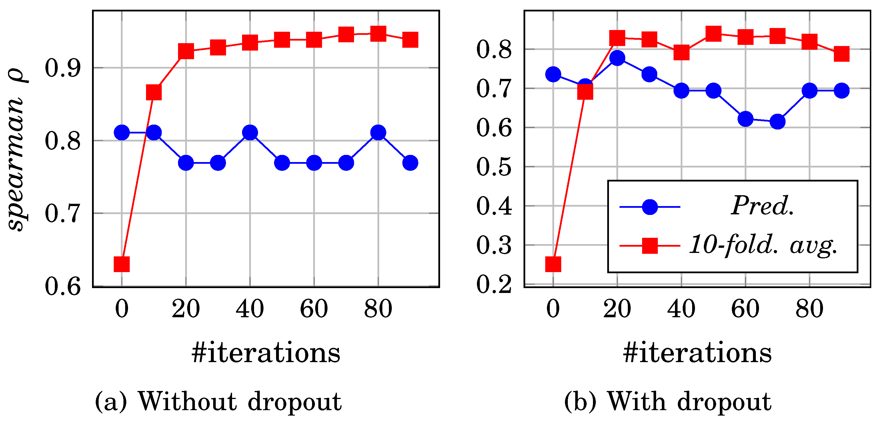
Dropout is applied as a regularization approach to enhance the PNN ranking stability by reducing over-fitting. We drop out the weights that have a probability of less than 0.5. these dropped weights are removed from FF, BP, and UW steps. The comparison between dropout and non-dropout of PNN are shown in Figure 16. The gap between the training model and ten-fold cross-validation curves has been reduced using dropout regularization using hyperparameters (l.r.=0.05, h.n.=100) on the iris data set. The dropout technique is used with all the data ranking results in the next section.
The following section is the evaluation of ranking experiments using label benchmark data sets.

6. Experiments

This section describes the classification and label ranking benchmark data sets, the results using PN and PNN, and a comparison with existing classification and ranking methods.

6.1. Data Sets

6.1.1. Image Classification Data Sets

PN is evaluated using CFAR-100 [54] and Fashion-MNIST [55] data sets.

6.1.2. Label Ranking Data sets

PNN is experimented with using three different types of benchmark data sets to evaluate the multi-label ranking performance. The first type of data set focuses on exception preference mining [56], and the `algae’ data set is the first type that highlights the indifference preferences problem, where labels have repeated preference value [57]. German elections 2005, 2009, and modified sushi are considered new and restricted preference data sets. The second type is real-world data related to biological science [18]. The third type of data set is semi-synthetic (SS) taken from the KEBI Data Repository at the Philipps University of Marburg [52]. All data sets do not have ranking ground truth, and all labels have a continuous permutation space of relations between labels. Table 2 summarizes the main characteristics of the data sets.

6.2. Results

6.2.1. Image Classification Results

PN has 3 kernel sizes of 5,10 and 20 and is tested on the CFAR-100 [54] data set and 1 kernel with a size 5 for Fashion-MNIST data set [55]. Table 3 shows the results compared to other convolutions networks.

6.2.2. Label Ranking Results

PNN is evaluated by restricted and non-restricted label ranking data sets. The results are derived using spearman  ρ and converted to Kendall τ coefficient for comparison with other approaches. For data validation, we used 10-fold cross-validation. To avoid the over-fitting problem, We used hyperparameters, i.e., l.r.= (0.0008,0.0005,0.005, 0.05, 0.1) hidden neuron = no.inputs+(5, 10, 50, 100, 200,300,400,450) neurons and scaling boundaries from 1 to 250) are chosen within each cross-validation fold by using the best l.r. on each fold and calculating the average τ of ten folds. Grid searching is used to obtain the best hyperparameter. For type B, we use three output groups and l.r.=0.001 and w b = 0.01 .

6.2.3. Benchmark Results

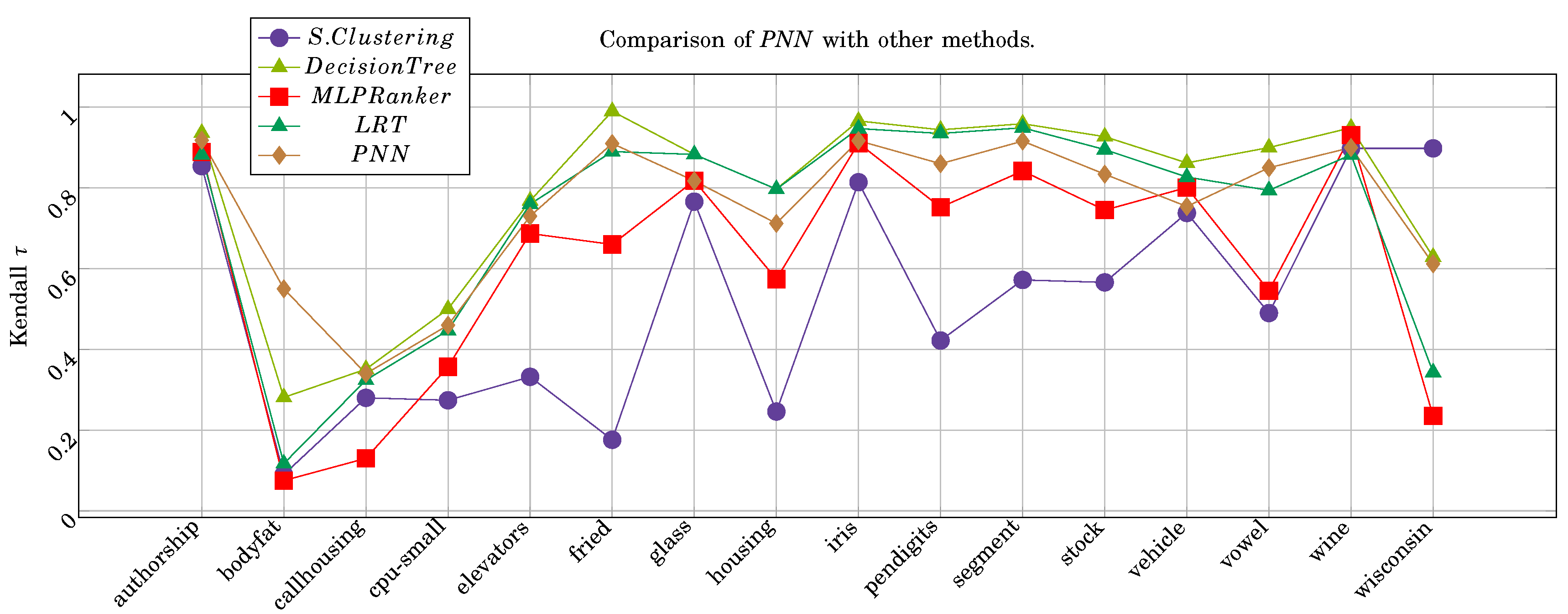
Table 4 summarizes PNN ranking performance of 16 strict label ranking data sets by l.r. and m.n. The results are compared with the four methods for label ranking; supervised clustering [58], supervised decision tree [52], MLP label ranking [23], and label ranking tree forest (LRT) [67]. Each method’s results are generated by ten-fold cross-validation. The comparison selects only the best approach for each method.
During the experiment, it was found that ranking performance increases by increasing the number of central neurons up to a maximum of 20 times the number of features. As shown in Table 6, The real datasets are ranked using PNN with dropout regulation due to complexity and over-fitting. The dropout requires increasing the number of epochs to reach high accuracy. All the results are held using a single hidden layer with various hidden neurons (100 to 450) and SS activation function. The Kendall τ error converges and reaches close to 1 after 2000 iterations, as shown in Figure 17.
Table 4 compares PNN with similar approaches used for label ranking. These approaches are; Decision trees [58], MLP-LR [23] and label ranking trees forest LRT [67]. In this comparison, we choose the method that has the best results for each approach.

6.2.4. Preference Mining Results

The ranking performance of the new preference mining data set is represented in Table 2. Two hundred fifty hidden neurons are used To enhance the ranking performance of the algae data set’s repeated label values. However, restricted labels ranking data sets of the same type, i.e., (German elections and sushi), did not require a high number of hidden neurons and incurred less computational cost.
Experiments on the real-world biological data set were conducted using supervised clustering (SC) [58], Table 5 presents the comparison between PNN and supervised clustering on biological real world data in terms of L o s s L R as given in Equation (11).
τ = 1 2 · L o s s L R
where τ is Kendall τ ranking error and L o s s L R is the ranking loss function.
SS function with 16 steps is used to rank Wisconsin data set with 16 labels. By increasing the number of steps in the interval and scaling up the features between -100 and 100, The step width is small. To enhance ranking performance, the data set has many labels. The number of hidden neurons is increased to exceed τ = 0.5 .
Table 5. Comparison between PNN and supervised clustered on biological real world data in terms of L o s s L R .
Biological real world data
DS S.Clustering PNN
cold 0.198 0.11
diau 0.304 0.255
dtt 0.124 0.01
heat 0.072 0.013
spo 0.118 0.014
Average 0.1632 0.0804
Table 6. PNN label ranking performance in terms of τ coefficient, learning step and the number of middle layer neurons (#m.n). The training per fold and testing time is given in the last two columns. ‘s’, ‘m’, ‘h’ denote seconds, minutes and hours, respectively.
Type DS Avg. τ #m.n. l.r. #Iterations. Dropout Scaling. Training t. Testing t.
Real cold 0.4 10 0.0008 2000 yes -4:4 2.8h 1.2s
diau 0.466 400 0.0005 2500 yes -2:2 2.9h 4s
dtt 0.60 400 0.0001 5000 yes -4:4 5.7h 1.88s
heat 0.876 450 0.0005 5000 yes -2:2 6.2h 1.18s
spo 0.8 300 0.0005 5000 yes -4:4 7.4h 0.98s
German2005 0.8 300 0.0005 1000 no -4:4 35.15m 0.0879s
German2009 0.67 300 0.0005 500 no -4:4 7.087m 0.105s
Semi-Synthesized authorship 0.931 200 0.0008 200 no -4:4 3.82m 0.34s
bodyfat 0.559 100 0.0005 2500 yes -2:2 16.92m 0.44s
calhousing 0.34 200 0.0007 1000 no -2:2 5.03h 4.127s
cpu-small 0.46 200 0.005 1000 no -2:2 2.089h 1.717
elevators 0.73 20 0.003 100 no -2:2 27.03m 3.7s
fried 0.89 100 0.005 100 no -2:2 1.02h 8.45s
glass 0.948 100 0.005 100 no -3:3 14.8s 0.04s
housing 0.7615 25 0.005 100 no -3:3 37.21s 0.1s
iris 0.956 100 0.005 100 no -3:3 29.39s 0.066s
pendigits 0.86 100 0.005 100 no -3:3 34.6m 5.69s
segment 0.956 20 0.007 100 no -3:3 440.8s 0.94s
stock 0.868 100 0.005 100 no -3:3 142.48s 0.87s
vehicle 0.869 100 0.005 100 no -3:3 91s 0.2s
vowel 0.85 100 0.005 100 no -3:3 88.37s 0.312s
wine 0.90 100 0.005 100 no -3:3 19.19s 0.063s
wisconsin 0.61 300 0.0005 2500 yes -4:4 13.56m 0.1332s

6.3. Computational Platform

PNN and PN is implemented from scratch without the Tensorflow API and developed using Numba API to speed the execution on the GPU and use Cuda 10.1 and Tensorflow-GPU 2.3 for GPU execution and executed at the University of Technology Sydney High-Performance Computing cluster based on Linux RedHat 7.7, which has an NVIDIA Quadro GV100 and memory of 32 G.B. For a non-GPU version of PNN is located at GitHub Repository [68].

6.4. Discussion and Future Work

It can be noticed from Table 2 that PN is performing better than ResNet [59] and WRN [60]. Different types of architectures of PN could be used to enhance the results and reach state-of-the-art in terms of image classification [69,70,71]. It can be noticed from Table 3 that PNN outperforms on SS data sets with τ A v g = 0.8 , whereas other methods such as, supervised clustering, decision tree, MLP-ranker and LRT, have results τ A v g = 0.79 , 0.73 , 0.62 , 0.475 , respectively. Also, the performance of PNN is almost 50% better than supervised clustering in terms of ranking loss function L o s s L R on real-world biological data set, as shown in Table 5. The superiority of PNN is used for classification and ranking problems. The ranking is used in input data as a feature selection criteria is a novel approach for deep learning.
Encoding the labels’ preference relation to numeric values and ranking the output labels simultaneously in one model is an advanced step over pairwise label ranking based on classification. PNN could be used to solve new preference mining problems. One of these problems is incomparability between labels, where Label ranking has incomparable relation , i.e., ranking space ( λ a λ b λ c ) is encoded to (1, 2, -1) and ( λ a λ b ) ( λ c λ d ) is encoded to (1, 2, -1, -2). PNN could be used to solve new problem of non-strict partial orders ranking, i.e., ranking space ( λ a λ b λ c ) is encoded to (1, 2, 3) or (1, 2, 2). Future research may enhance PN by adding kernel size and SS parameters as part of the deep learning to choose the best kernel size and SS step width, which could enhance the image attention. Modifying PNN architecture by adding bias and solving noisy label ranking problems.

7. Conclusions

This paper proposed a novel method to rank a complete multi-label space in output labels and features extraction in both simple and deep learning.PN is a new research direction for image recognition based on new kernel and pixel calculations. PNN and PN are native ranker networks for image classification and label ranking problems that uses SS or PSS to rank the multi-label per instance. This neural network’s novelty is a new kernel mechanism, activation, and objective functions. This approach takes less computational time with a single middle layer. It is indexing multi-labels as output neurons with preference values. The neuron output structure can be mapped to integer ranking value; thus, PNN accelerates the ranking learning by assigning the rank value to more than one output layer to reinforce updating the random weights. PNN is implemented using python programming language 3.6 [68], and activation functions are modelled using wolframe Mathematica software [72]. A video demo that shows the ranking learning process using toy data is available to download [48].

Acknowledgments

This work was supported in part by the Australian Research Council (ARC) under discovery grants DP180100656 and DP210101093. The research was also sponsored in part by the US Office of Naval Research Global under Cooperative Agreement Number ONRG - NICOP - N62909-19-1-2058 and AFOSR – DST Australian Autonomy Initiative agreement ID10134. We also thank the NSW Defence Innovation Network and NSW State Government of Australia for financial support in part of this research through grant PP21-22.03.02.

References

  1. Frnkranz, J.; Hüllermeier, E. Preference Learning, 1st ed; Springer-Verlag: Berlin/Heidelberg, Germany, 2010. [Google Scholar]
  2. Brafman, R.; Domshlak, C. Preference handling - an introductory tutorial. 2009; pp. 58–86.
  3. Adomavicius, G.; Tuzhilin, A. Toward the next generation of recommender systems: a survey of the state-of-the-art and possible extensions. 2005; pp. 734–749.
  4. Montaner, M.; López, B. A taxonomy of recommender agents on the internet. 2003; pp. 285–330.
  5. Aiolli, F. A preference model for structured supervised learning tasks. 2005; pp. 557–560.
  6. Crammer, K.; Singer, Y. Pranking with ranking. 2002; pp. 641–647.
  7. Ni, Q.; Guo, J.; Wu, W.; Wang, H. Influence-based community partition with sandwich method for social networks. IEEE Trans. Comput. Soc. Syst. 2022, 10, 819–830. [Google Scholar] [CrossRef]
  8. Wang, H.; Gao, Q.; Li, H.; Wang, H.; Yan, L.; Liu, G. A Structural Evolution-Based Anomaly Detection Method for Generalized Evolving Social Networks. Comput. J. 2020, 65, 1189–1199. [Google Scholar] [CrossRef]
  9. Huang, C.-Q.; Jiang, F.; Huang, Q.-H.; Wang, X.-Z.; Han, Z.-M.; Huang, W.-Y. Dual-graph attention convolution network for 3-d point cloud classification. IEEE Trans. Neural Netw. Learn. Syst. 2022, 1–13. [Google Scholar] [CrossRef] [PubMed]
  10. Wang, H.; Cui, Z.; Liu, R.; Fang, L.; Sha, Y. A multi-type transferable method for missing link prediction in heterogeneous social networks. IEEE Trans. Knowl. Data Eng. 2022, 35, 10981–10991. [Google Scholar] [CrossRef]
  11. Guo, F.; Zhou, W.; Lu, Q.; Zhang, C. Path extension similarity link prediction method based on matrix algebra in directed networks. Comput. Commun. 2022, 187, 83–92. [Google Scholar] [CrossRef]
  12. Qin, X.; Liu, Z.; Liu, Y.; Liu, S.; Yang, B.; Yin, L.; Liu, M.; Zheng, W. User ocean personality model construction method using a bp neural network. Electronics 2022, 11, 3022. [Google Scholar] [CrossRef]
  13. Liu, L.; Zhang, S.; Zhang, L.; Pan, G.; Yu, J. Multi-uuv maneuvering counter-game for dynamic target scenario based on fractional-order recurrent neural network. IEEE Trans. Cybern. 2022, 53, 4015–4028. [Google Scholar] [CrossRef] [PubMed]
  14. Zhou, Y.; Liu, Y.; Yang, J.; He, X.; Liu, L. A taxonomy of label ranking algorithms. JCP 2014, 9, 557–565. [Google Scholar] [CrossRef]
  15. Furnkranz, J.; Hüllermeier, E. Pairwise preference learning and ranking in machine learning. 2003; pp. 145–156.
  16. Fürnkranz, J.; Hüllermeier, E. Preference learning. 2010.
  17. Har-Peled, S.; Roth, D.; Zimak, D. Constraint classification: A new approach to multiclass classification. 2002.
  18. Hüllermeier, E.; Furnkranz, J.; Cheng, W.; Brinker, K. Label ranking by learning pairwise preferences. 2008; pp. 1897–1916.
  19. Furnkranz, J.; Hüllermeier, E. Decision tree modeling for ranking data. 2011; pp. 83–106.
  20. Cheng, W.; Hüllermeier, E. Instance-based label ranking using the mallows model. 2008; pp. 143–157.
  21. Mihajlo, G.; Nemanja, D.; Slobodan, V. Learning from pairwise preference data using gaussian mixture model. 2014.
  22. Burges, T.S.C. Learning to rank using gradient descent. 2005; pp. 58–86.
  23. Ribeiro, G.; Duivesteijn, W.; Soares, C.; Knobbe, A. Multilayer perceptron for label ranking. In Proceedings of the 22nd International Conference on Artificial Neural Networks and Machine Learning - Volume Part II; Springer: Berlin/Heidelberg, Germany, 2012; pp. 25–32. [Google Scholar]
  24. Freund, Y.; Iyer, R.; Schapire, R.E.; Singer, Y. ; An efficient boosting algorithm for combining preferences. J. Mach. Learn. Res. 2003, 4, 933–969. [Google Scholar]
  25. Wu, Q.; Burges, C.J.; Svore, K.M.; Gao, J. Adapting boosting for information retrieval measures. Learn. Rank. Inf. Retr. 2010, 13, 254–270. [Google Scholar] [CrossRef]
  26. Jian, Y.; Xiao, J.; Cao, Y.; Khan, A.; Zhu, J. Deep pairwise ranking with multi-label information for cross-modal retrieval. In 2019 IEEE International Conference on Multimedia and Expo (ICME), 2019; pp. 1810–1815.
  27. Li, J.; Wing, W.Y.N.; Xing, T.; Kwong, S.; Wang, H. Weighted multi-deep ranking supervised hashing for efficient image retrieval. Int. J. Mach. Learn. Cybern. 2020, 11, 883–897. [Google Scholar] [CrossRef]
  28. Ji, Z.; Cui, B.; Li, H.; Jiang, Y.-G.; Xiang, T.; Hospedales, T.; Fu, Y. Deep ranking for image zero-shot multi-label classification. IEEE transactions on image processing : A publication of the IEEE Signal Processing Society.
  29. Cherian, A.K.; Poovammal, E. Classification of remote sensing images using cnn. IOP Conference Series: Materials Science and Engineering, 1130. [Google Scholar]
  30. Singh, A.R.; Athisayamani, S. Survival prediction based on brain tumor classification using convolutional neural network with channel preference,” in Data Engineering and Intelligent Computing, V. Bhateja, L. Khin Wee, J. C.-W. Lin, S. C. Satapathy, and T. M. Rajesh, Eds.; Springer: Singapore, 2022; pp. 259–269. [Google Scholar]
  31. Lv, Z.; Qiao, L.; Li, J.; Song, H. Deep-learning-enabled security issues in the internet of things. IEEE Internet Things J. 2021, 8, 9531–9538. [Google Scholar] [CrossRef]
  32. Lv, Z.; Yu, Z.; Xie, S.; Alamri, A. Deep learning-based smart predictive evaluation for interactive multimedia-enabled smart healthcare. ACM Trans. Multimedia Comput. Commun. Appl. 2022, 18, 1. [Google Scholar] [CrossRef]
  33. Xu, J.; Pan, S.; Sun, P.Z.H.; Park, S.H.; Guo, K. Human-factors-in-driving-loop: Driver identification and verification via a deep learning approach using psychological behavioral data. IEEE Trans. Intell. Transp. Syst. 2023, 24, 3383–3394. [Google Scholar] [CrossRef]
  34. Zhan, C.; Dai, Z.; Soltanian, M.R.; de Barros, F.P.J. Data-worth analysis for heterogeneous subsurface structure identification with a stochastic deep learning framework. Water Resour. Res. 2022, 58, e2022WR033241. [Google Scholar] [CrossRef]
  35. Pare, S.; Mittal, H.; Sajid, M.; Bansal, J.C.; Saxena, A.; Jan, T.; Pedrycz, W.; Prasad, M. Remote sensing imagery segmentation: A hybrid approach. Remote Sens. 2021, 13, 4604. [Google Scholar] [CrossRef]
  36. Moraga, C.; Heider, R. New lamps for old!" (generalized multiple-valued neurons). In Proceedings 1999 29th IEEE International Symposium on Multiple-Valued Logic (Cat. No. 99CB36329); IEEE: 1999; pp. 36–41.
  37. Aizenberg, I.; Aizenberg, N.; Vandewalle, J.P. Multi-Valued and Universal Binary Neurons: Theory, Learning and Applications; Kluwer Academic Publishers: Norwell, MA, USA, 2000. [Google Scholar]
  38. Zhou, W.; Lv, Y.; Lei, J.; Yu, L. Global and local-contrast guides content-aware fusion for rgb-d saliency prediction,” IEEE Trans. Syst. Man Cybern. Syst. 2021, 51, 3641–3649. [Google Scholar] [CrossRef]
  39. Xie, B.; Li, S.; Li, M.; Liu, C.H.; Huang, G.; Wang, G. Sepico: Semantic-guided pixel contrast for domain adaptive semantic segmentation. IEEE Trans. Pattern Anal. Mach. Intell. 2023, 1–17. [Google Scholar] [CrossRef]
  40. Zhang, X.; Huang, D.; Li, H.; Zhang, Y.; Xia, Y.; Liu, J. Self-training maximum classifier discrepancy for eeg emotion recognition. CAAI Transactions on Intelligence Technology.
  41. Jiang, F.; Kong, B.; Li, J.; Dashtipour, K.; Gogate, M. Robust visual saliency optimization based on bidirectional markov chains. Cogn. Comput. 2020, 1–12. [Google Scholar] [CrossRef]
  42. Gupta, A.K.; Seal, A.; Prasad, M.; Khanna, P. Salient object detection techniques in computer vision—a survey. Entropy 2020, 22, 1174. [Google Scholar] [CrossRef]
  43. Lei, H.; Lei, T.; Yue-nian, T. Sports image detection based on particle swarm optimization algorithm. Microprocess. Microsystems 2021, 80, 103345. [Google Scholar] [CrossRef]
  44. Zhang, K.; Wang, Z.; Chen, G.; Zhang, L.; Yang, Y.; Yao, C.; Wang, J.; Yao, J. Training effective deep reinforcement learning agents for real-time life-cycle production optimization. J. Pet. Sci. Eng. 2022, 208, 109766. [Google Scholar] [CrossRef]
  45. Liu, M.; Gu, Q.; Yang, B.; Yin, Z.; Liu, S.; Yin, L.; Zheng, W. Kinematics model optimization algorithm for six degrees of freedom parallel platform. Appl. Sci. 2023, 13, 5. [Google Scholar] [CrossRef]
  46. Zhou, G.; Zhang, R.; Huang, S. Generalized buffering algorithm. IEEE Access 2021, 9, 140–227. [Google Scholar] [CrossRef]
  47. Zhang, R. Sports action recognition based on particle swarm optimization neural networks. Wireless Communications and Mobile Computing.
  48. Elgharabawy, A. Preference neural network convergence performance. 2020. https://drive.google.com/drive/folders/1yxuqYoQ3Kiuch-2sLeVe2ocMj12QVsRM?usp=sharing.
  49. Bologna, G. Rule extraction from a multilayer perceptron with staircase activation functions. 2000.
  50. Kendall, M. Rank correlation methods. 1948.
  51. Spearman, C. The proof and measurement of association between two things. Am. J. Psychol. 1904, 15, 72–101. [Google Scholar] [CrossRef]
  52. Cheng, W.; Hühn, J.; Hxuxllermeier, E. Decision tree and instance-based learning for label ranking. In Proceedings of the 26th Annual International Conference on Machine Learning, 2009, ser. ICML ’09. ACM; pp. 161–168.
  53. LeCun, Y.; Cortes, C. MNIST handwritten digit database. 2010. Available: http://yann.lecun.com/exdb/mnist/.
  54. Krizhevsky, A. Learning multiple layers of features from tiny images. Tech. Rep. 2009. [Google Scholar]
  55. Xiao, H.; Rasul, K.; Vollgraf, R. Fashion-mnist: a novel image dataset for benchmarking machine learning algorithms. 2017. http://arxiv.org/abs/1708.07747.
  56. de S<i>a</i>´, C.R.; Duivesteijn, W. Discovering a taste for the unusual: exceptional models for preference mining. 2018; pp. 1775–1807.
  57. Cláudio, R. algae dataset. 2018. [CrossRef]
  58. Grbovic, M.; Djuric, N.; Guo, S.; Vucetic, S. Supervised clustering of label ranking data using label preference information. Mach. Learn. 2013, 93, 191–225. [Google Scholar] [CrossRef]
  59. He, K.; Zhang, X.; Ren, S.; Sun, J. Deep residual learning for image recognition. In 2016 IEEE Conference on Computer Vision and Pattern Recognition (CVPR), 2016; pp. 770–778.
  60. Zagoruyko, S.; Komodakis, N. Wide residual networks. ArXiv, 1605. [Google Scholar]
  61. Huang, G.; Liu, Z.; Maaten, L.D.; Weinberger, K.Q. Densely connected convolutional networks. In 2017 IEEE Conference on Computer Vision and Pattern Recognition (CVPR), 2017; pp. 2261–2269.
  62. Tan, M.; Le, Q.V. Efficientnetv2: Smaller models and faster training,” arXiv 2021, abs/2104. 0 0298.
  63. Ridnik, T.; Sharir, G.; Ben-Cohen, A.; Ben-Baruch, E.; Noy, A. Ml-decoder: Scalable and versatile classification head. 2021.
  64. Wu, H.; Xiao, B.; Codella, N.C.F.; Liu, M.; Dai, X.; Yuan, L.; Zhang, L. Cvt: Introducing convolutions to vision transformers. 2021 IEEE/CVF International Conference on Computer Vision (ICCV).
  65. Zhang, K. Lstm: An image classification model based on fashion-mnist dataset. 2018.
  66. Tanveer, M.; Khan, M.U.K.; Kyung, C.M. Fine-tuning darts for image classification. 2020 25th International Conference on Pattern Recognition (ICPR), 4789. [Google Scholar]
  67. de Sá, C.R.; Soares, C.; Knobbe, A.; Cortez, P. Label ranking forests. Expert Syst. J. Knowl. Eng. 2017, 34. [Google Scholar] [CrossRef]
  68. Elgharabawy, A. Preference neural network source code,” Python Code, Mathematica code, 2022. https://github.
  69. Meena, M.S.; Singh, P.; Rana, A.; Mery, D.; Prasad, M. A.; Mery, D.; Prasad, M. A robust face recognition system for one sample problem. In Image and Video Technology; Lee, C., Su, Z., Sugimoto, A., Eds.; Springer International Publishing: Cham, Switzerland, 2019; Mery, D.; pp. 13–26. [Google Scholar]
  70. Rajora, S.; Vishwakarma, D.k.; Singh, K.; Prasad, M. Csgi: A deep learning based approach for marijuana leaves strain classification,” in 2018 IEEE 9th Annual Information Technology, Electronics and Mobile Communication Conference (IEMCON), 2018; pp. 209–214.
  71. Padmanabha, A.A.; Appaji, M.A.; Prasad, M.; Lu, H.; Joshi, S. Classification of diabetic retinopathy using textural features in retinal color fundus image. In 2017 12th International Conference on Intelligent Systems and Knowledge Engineering (ISKE), 2017; pp. 1–5.
  72. Wolfram Research, Inc., Mathematica. Wolfram. https://www.wolfram.
Figure 1. PSS activation function where n = 3 and step width w = 1 and c = 100 and 5 in (a,b) respectively.
Preprints 71295 g001
Figure 2. SS activation function where n = 6 , 30 and 20 and boundary b = 1 , 30 and 1 and scale factor for the decimal place is s = 1 , 1 and 10 for ranking/classification, extreme label ranking/classification and regression in (ac) respectively.
Preprints 71295 g002
Figure 4. Multiple layer label ranking comparison of benchmark data sets [52] results using the PNN and SS functions after 100 epochs and learning rate = 0.007.
Preprints 71295 g004
Figure 5. The structure of preference neuron where φ n = 4 .
Preprints 71295 g005
Figure 7. The structure used in both ranker ANN and PNN where φ n = 3 , f i n = 3 and λ o u t = 3 , per x 1 , π 1 , L { λ a , λ b , λ c } where π 1 = { 1 , 2 , 3 } . and comparison of the convergence for both NN’s. The demo video of convergence of two NN in the link [48].
Preprints 71295 g007
Figure 8. Image pixel sorting for the flattened windows in (a,b) respectively.
Preprints 71295 g008
Figure 9. Sample of moving objects in (a,b) without and with averaging by window 2x2. The ranking of two flattened images are ρ = 0.216 and 0.79 in (a,b), respectively. Sample of moving noisy object in (c,d) without and with image averaging by a window of 2x2. The ranking of two flattened images are ρ = 0.137 , 0.75 and 0.75 in (c,d) respectively. ranking scaled circle in (e,f), respectively.
Preprints 71295 g009
Figure 10. Detecting the similarity in remote sensing and face recognition by ranking the image pixels after averaging the pixels using a 2x2 window.
Preprints 71295 g010
Figure 11. The PN structure has three kernels and three PNNs where φ n = 2 , f 1 i n = 16 , f 2 i n = 81 , f 3 i n = 169 and λ o u t = 15 , per x 1 , π 1 , π { λ 1 , λ 2 , λ 3 , λ 15 }.
Preprints 71295 g011
Figure 12. Visualizing the ranking of stock dataset [52] has five labels using SS activation function of stock data set at epoch 0 and 3900 in (a,b) respectively.
Preprints 71295 g012
Figure 13. PNN activation function comparison using complete labels and 60% missing labels in (a,b), respectively.
Preprints 71295 g013
Figure 14. ROC of three labels ranking on the wine data set using PNN h.n=100 and 50 epochs.
Preprints 71295 g014
Figure 15. The confusion matrix of testing the wine, glass data sets where τ = 0.947, 0.84, Accuracy = 0.935 and 0.8 in (a,b) respectively.
Preprints 71295 g015
Figure 16. Training and validation performance without and with dropout regulation approach in (a,b) respectively.
Preprints 71295 g016
Figure 17. Ranking performance comparison of PNN with other approaches.
Preprints 71295 g017
Table 1. ANN types used in initial experiment.
Type Ranker ANN PNN
Activation Fun. ReLU,Sigmoid PSS, SS
Gradient Descent Ascent
Objective Fun. RMS ρ
Stopping Criteria. τ ρ
Table 2. Benchmark data sets for label ranking; preference mining [57], real-world data sets [58] and semi-synthetic (s-s) [52].
Type DS Cat. #Inst. #Attr. #lbl.
Mining algae chemical stat. 317 11 7
german.2005 user pref. 413 31 5
german.2009 user pref. 413 31 5
sushi user pref. 5000 13 7
top7movies user pref. 602 7 7
Real cold biology 2,465 24 4
diau biology 2,465 24 7
dtt biology 2,465 24 4
heat biology 2,465 24 6
spo biology 2,465 24 11
Semi-Synthesized authorship A 841 70 4
bodyfat B 252 7 7
calhousing B 20,640 4 4
cpu-small B 8192 6 5
elevators B 16,599 9 9
fried B 40,769 9 5
glass A 214 9 6
housing B 506 6 6
iris A 150 4 3
pendigits A 10,992 16 10
segment A 2310 18 7
stock B 950 5 5
vehicle A 846 18 4
vowel A 528 10 11
wine A 178 13 3
wisconsin B 194 16 16
Table 3. Comparison of classification on CIFAR-100 [54] and Fashion-Mnist data set [55] using different convolution models
DS Model Baseline MixUp
CIFAR-100 ResNet [59] 72.22 78.9
WRN [60] 78.26 82.5
Dense [61] 81.73 83.23
EfficientNetV2-M [62] 92.2 -
EffNet-L2 (SAM) [63] 96.08 -
CvT [64] 94.39 -
PrefNet 80.6 -
Fashion-MNIST MLP 0.871 -
RandomForest 0.873 -
LogisticRegression 0.842 -
SVC 0.897 -
SGDClassifier 0.81 -
LSTM [65] 0.8757 -
DART [66] 0.965 -
PrefNet 0.91 -
Table 4. PNN performance comparison with various approaches: supervised clustering [58], supervised decision tree [52], MLP label ranking [23] and label ranking tree forest (LRT) [67].
Label Ranking Methods
DS S.Clust. DT MLP-LR LRT PNN
authorship 0.854 0.936(IBLR) 0.889(LA) 0.882 0.918
bodyfat 0.09 0.281(CC) 0.075(CA) 0.117 0.5591
calhousing 0.28 0.351(IBLR) 0.130(SSGA) 0.324 0.34
cpu-small 0.274 0.50(IBLR) 0.357(CA) 0.447 0.46
elevators 0.332 0.768(CC) 0.687(LA) 0.760 0.73
fried 0.176 0.99(CC) 0.660(CA) 0.890 0.91
glass 0.766 0.883(LRT) 0.818(LA) 0.883 0.8175
housing 0.246 0.797(LRT) 0.574(CA) 0.797 0.712
iris 0.814 0.966(IBLR) 0.911(LA) 0.947 0.917
pendigits 0.422 0.944(IBLR) 0.752(CA) 0.935 0.86
segment 0.572 0.959(IBLR) 0.842(CA) 0.949 0.916
stock 0.566 0.927(IBLR) 0.745(CA) 0.895 0.834
vehicle 0.738 0.862(IBLR) 0.801(LA) 0.827 0.754
vowel 0.49 0.90(IBLR) 0.545(CA) 0.794 0.85
wine 0.898 0.949(IBLR) 0.931(LA) 0.882 0.90
wisconsin 0.09 0.629(CC) 0.235(CA) 0.343 0.612
Average 0.475 0.79 0.621 0.730 0.755
Disclaimer/Publisher’s Note: The statements, opinions and data contained in all publications are solely those of the individual author(s) and contributor(s) and not of MDPI and/or the editor(s). MDPI and/or the editor(s) disclaim responsibility for any injury to people or property resulting from any ideas, methods, instructions or products referred to in the content.
Copyright: This open access article is published under a Creative Commons CC BY 4.0 license, which permit the free download, distribution, and reuse, provided that the author and preprint are cited in any reuse.
Prerpints.org logo

Preprints.org is a free preprint server supported by MDPI in Basel, Switzerland.

Subscribe

© 2024 MDPI (Basel, Switzerland) unless otherwise stated