
Submitted:
31 August 2023
Posted:
31 August 2023
You are already at the latest version
Abstract
With an explosion of data in the nearly every domain, from physical and environmental sciences to econometrics and even social science, we have entered a golden era of time-domain data science. In addition to ever increasing data volumes and varieties of time-series, there's a plethora of techniques available to analyses them. Unsurprisingly, machine learning approaches are very popular. In environmental sciences (ranging from climate studies to space weather/solar physics), machine learning (ML )and deep learning (DL) approaches complement the traditional data assimilation approaches. In solar and astrophysics, multiwavelength time-series or lightcurves along with observations of other messengers like gravitational waves provide a treasure trove of time-domain data for ML/DL approaches for modeling and forecasting. In this regard, deep learning algorithms such as recurrent neural networks (RNNs) should prove extremely powerful for forecasting as it has in several other domains. Such methods agnostic of the physics can only predict transient flares that are represented in the original distribution trained on (eg. coloured noise fluctuations) and not special, isolated episodes (eg. a one-off outburst like a major coronal mass ejection) potentially distinguishing them. Therefore it is vital to test robustness of these techniques ; here we attempt to make a small contribution to this by exploring sensitivity of RNNs with some rudimentary experiments. We test the performance of a very successful class of RNNs, the Long Short Term Memory (LSTM) algorithms with simulated lightcurves. As an example, we focus on univariate forecasting of time-series (or lightcurves) characteristic certain variable astrophysical objects (eg. active galactic nuclei or AGN). Specifically, we explore the sensitivity of training and test losses to key parameters of the LSTM network and data characteristics namely gaps and complexity measured in terms of number of Fourier components. We find that typically, the performances of LSTMs are better for pink or flicker noise type sources. The key parameters on which performance is dependent are batch size for LSTM and the gap percentage of the lightcurves. While a batch size of $10-30$ seems optimal, the most optimal test and train losses are under $10 \%$ of missing data for both periodic and random gaps in pink noise. The performance is far worse for red noise. This compromises detectability of transients. Thus, we show that generative models (time-series simulations) are excellent guides for use of RNN-LSTMs in building forecasting systems
Keywords:
recurrent neural networks
; LSTM
; lightcurves
; simulation
; variability
1. Introduction
Time domain data science is a rapidly growing field with problems ranging from "physics-based" time-dependent modeling of driving processes to the model independent forecasting of transients. Traditionally, physical and environmental sciences including meteorology, solar and astrophysics, has been a field where modeling of observational data is done with a theoretical or phenomenological, physics-based model. For forecasting, statistical techniques like the Kalman Filter, autoregressive models, etc. have been used with data assimilation encompassing the suite of cutting edge methods used in meteorology. With ever increasing volumes, velocities and varieties of time domain data, from contemporaneous observations, fast and precise forecasting is becoming increasingly important. Especially, real time alerts that are auto-generated is a challenge with the sheer volume and velocity of data flow. And this challenge is particularly pronounced in astronomy which affords some of the highest values of volume and velocity. With the next generation of observatories like CTA in gamma-rays [for eg., [1,2,3], SKA in radio [for eg., [4,5,6], LSST in optical [for eg., [7], this exact approach is not practical and in some situation not possible to implement. LSST is expected to produce alerts per night. SKA will receive few Petabytes (PBs) of raw data per second from the telescopes and the data and signal processors will have to handle a few Terabytes per second. This will translate into a very high rate of transient signals. At such large rates and volumes, we need automated, fast and efficient and intelligent systems to process and interpret such alerts. Probabilistic forecast of a future episode based on current and / or past observations at different wavelengths would constitute alerts. Target of Opportunity (ToO) observations stand to benefit from machine intelligence in this respect. Traditionally ToO observations sent under MoU agreements between collaborations running different telescopes, astronomer’s telegrams, virtual observatory events or VOEvents 1, which are automatically parsed as also preplanned observations coordinated by representatives of different telescope collaborations. Furthermore, the variety of transient signals makes it inevitable to use machine learning techniques [eg., [7,8,9,10] to detect complex patterns and classes of signals. In particular, methods of deep learning are particularly relevant in capturing the complex variability behaviour of astronomical signals [11,12]. The vast majority of existing efforts are focussed on classifying transients from a population. While, one can classify the variability in lightcurves or in general any time-series broadly into stochastic, (quasi-)periodic, secular and transients, the exact pattern of variations can be quite complex to both model and predict. That is why it is equally important to focus on individual lightcurves and test the ability of machine / deep learning methods in capturing the complexity and individuality of lightcurves as also the generalisation capability to a variety of lightcurves. In this work we will focus on the former with a view to building towards the latter.
Compared to astronomical signals, even the more elaborate datasets of solar outbursts - flares and coronal mass ejections (CMEs) - the meteorological datasets such as atmospheric or oceanographic data are vastly more complex. Not only do they have spatio-temporal features (true also for solar data), the resolution required to make impactful predictions are significantly finer. This poses a challenge not only for the data scientific techniques but also for the underlying models (numerical/physical). Often for numerical weather prediction, convective processes (atmosphere) require separate numerical schemes for the physical models from the coarse-grained global circulation models or GCMs [eg., [13] 2. Thus meteorological data and the requirements of meteorological forecasting present greater challenges than astronomical forecasting. Furthermore, the principle approach(es) of numerical weather prediction center around data assimilation [14] - which involves optimally combining observed information with the theoretical (most likely numerical) model - including for operations at weather and climate prediction centres like the Met-Office and European Centre for for Medium-Range Weather Forecasts (ECMWF). Therefore, for testing basic features of machine learning / deep learning methods, astronomical datasets may have an advantage. And hence, we focus on them here, with the hope that some of the fundamental insights or indeed challenges would hold true in general, for more complicated scenarios.
Astrophysical variability is often in the low signal to noise ratio regime making it a more challenging one. Some of the most important forecast problems for astronomical time-series are for transient flares and quasi-periodic oscillations that are buried under stochastic signals. Note that the stochasticity or noisy component is actually a combination of background noise either due to instrumental or observational backgrounds and a genuine astrophysical component related to stochastic processes in the transient source. This constitutes an interesting forecasting challenge. Prediction of noisy time-series is certainly not limited to astronomy. In fact, important applications appear in the fields of finance [15], meteorology [16], neuroscience, etc. As explained in Lee Giles and Lawrence [17], in general, forecasting from limited sample sizes in a low signal to noise, highly non-stationary and non-linear setting is enormously challenging. And in this most general scenario, Lee Giles and Lawrence [17] prescribes combination of symbolic representation with a self-organising map and grammatical inference with recurrent neural networks (RNNs) [18]. In our case of astrophysical signals, while we maybe in the high noise regime, the non-linearity and non-stationarity can be assumed to be weak in most typical cases. Therefore, we simply use RNNs. While we do not wish to draw conclusions and see patterns and trends by over-fitting a unwanted noise in the lightcurves, we do wish to study outbursts that emerge at short timescale of the noise spectrum. In fact, a key question in variability in AGNs is distinguishing between statistical fluctuations that in extreme cases lead to occasional outbursts and a special event isolated from these underlying fluctuations and thus drawn from a different physical process or distribution equivalently. An agnostic learning algorithm should be able to predict the former but not the latter. In order to do this, we must broadly characterise the response of RNN architecture to noise characteristics. This is clearly relevant in predicting a well defined transient episode like an outburst or flaring episode or a potential quasi-periodic signal in advance in real astronomical observations.
A key part of time domain astronomy involves setting up multiwavelength observational campaigns. These are either pre-planned medium to long term observation or target of opportunity observations (ToOs) often triggered by an episode of transient activity at one wavelength. In either case, a key ingredient is the ability to use existing observations to predict future ones. These existing observations are either simply past observations of the same wavelength or more interestingly those at another wavelength. The latter presumes a physical model that generates multiwavelength emission with temporal lags between different wavebands. This presents a forecasting problem tailored for application of RNNs and deep learning in general. Most of the applications of machine learning in transient astronomy are focussed on the classification of transients (either source or variability type) [19]. Here we look at time-domain forecasting along the lines of that in finance, econometrics, numerical weather prediction (NWP), etc. Specifically, multiwavelength transient astronomy may be viewed as a multivariate forecasting.
One of the keys to such forecasting is understanding, as best as we can, the performance of the algorithm in presence of different types of temporal structures. And the quantification of the performance is done in terms of training and test losses.
There are several predictive frameworks for time-series, machine learning and otherwise. A number of time-series models are in use across domains 3, such as Holt-Winters [20], ARIMA and SARIMA [21], GARCH [22], etc. Typically the Autoregressive Integrated Moving Average (ARIMA) models are most popularly used for forecasting in several domains with the "Integrated" part dealing with the large scale trends. For detecting features and patterns, supervised machine learning algorithms such as Random Forest [23], Gradient Boosting Machine [24], etc. Viewing the problem as a regression problem one can use Lasso Regression, Neural Networks, etc. In this paper, we do not attempt to provide a comprehensive survey on the various time-series forecasting methods and their efficacy for forecasting in domains modest signal-to-noise domains like astronomy. Rather we focus on one of the most popular methods that has yielded success for long-term time-series data. In this respect, recurrent neural networks (RNNs) are an excellent candidate [18].
RNNs like other neural networks have the capabilities of handling complex, non-linear dependencies. But unlike other networks, its "directed cyclic" nature, which allows the input signal at any stage to be fed back to itself suitable for time-series work. In particular, we focus Long Short-Term Memory RNNs architectures (LSTM) [25] which are capable of keeping track of long-term dependencies. This is clearly important in astronomy with the rather large dynamic range of timescales of underlying physical processes as well as observations. In order to do this, we test with artificial datasets that do not have a very complex temporal structure. More significantly, we use artificial datasets with characteristics typically found in long term astronomy observations and that we have some apriori knowledge of.
We subdivide the work into the following sections. In Section 2, we review the basic or core architecture of the RNN-LSTM used. The following Section 3 provides the science case of multiwavelength forecasting motivating the methodological work. The so-called sensitivity tests in two sections. In subSection 4.1, we examine the effects of dataset characteristics, gaps and complexity in terms of fourier components on performance. In subSection 4.2, we examine dependencies on the neural network (hyper)parameters. We apply our learning to the example of real-time statistical forecast of a transient flare while it develops in Section 5. Finally we put forth our conclusions in Section 6.
2. Overview : Recurrent Neural Network with Long Short Term Memory Architecture
Here we describe the structure of the forecasting machinery used. Astronomical time-series or lightcurves especially those that are obtained from long term monitoring campaigns tend to have correlations over a wide range of timescales ranging from minutes to years. Given the capacity of RNN-LSTMs to retain longer term memory of any process and use it in forecasting [25], we wish to perform our sensitivity tests on this method. In order to do so, we need to understand the neural network framework and start with an overview of the RNN-LSTM network architecture in the following subSection 2.1 and Section 2.2.
2.1. Memory Cell Block Structure
In RNNs, the inputs are fed to blocks that combine the inputs and perform logistic regression to produce an output. Within LSTMs, these blocks also act as a "memory unit" as they store input states from previous blocks. This block that performs this function is the so-called memory cell block. Each LSTM block of the network architecture has the standard design as found in the literature [26]4 5 and can have multiple memory cells with the same input and same output. The blocks representing a stage t, have input, and output, . The complex architecture within a block as shown in Figure 1, enables the network to retain memory of previous stages which ultimately can be used to factor in long term dependencies. There are multiple gates which are represented by the sigmoid function, , which determine whether the signal or input to it is passed on or suppressed. There are three such gates : forget, , input, and output, . First, the output from the previous stage, is combined with the input at the current stage, to give . This represents the internal state before passing through the LSTM block structure at stage t. The forget gate determines if this internal state, is passed on or forgotten at the next stage t. Similarly, the input gate determines the same for the internal state at stage t, . These are then combined to update the current internal state a as . This updated internal state is then passed through another sigmoid, the output gate which determines how much of this state is passed on to the next stage, , as .
2.2. Network Structure and (Hyper)-Parameters
Having seen the inner working of an LSTM block, we look at the RNN network itself, reminding the reader of the structure and terminology used in deep learning. In an RNN network, the basic structure consists of layers of memory cell blocks as shown in Figure 2. There is an input layer and one output layer. In between these there are one or more hidden layers. The inputs from the first layer are in general connected to those in the next hidden layer, which in turn are connected to the next layer and so on. In our application of time-series forecasting input vector is essentially a univariate time-series. When this simplest RNN unit is rolled out, we can visualise the individual time-steps as shown in Figure 1. So for multivariate and therefore multiwavelength forecasting, we will have multiple inputs as in Figure 2. The blocks of the final layer are then connected to the output layer. These inputs or a superposition of them in general, go through logistic regression and accordingly impact the block they connect to. In general, each layer has their own weights and biases in the superposition of "inputs" from the previous layers. However, for RNNs, the relation between successive inputs is built into the equations governing the network at the level of blocks as described above.
This network architecture is what is typically used in forecasting time-series or sequential data in general. We build the RNN with multiple LSTM layers with 3-dimensional input namely samples, time step and features. The samples represent the no. of data points in the time-series. The features are the no. of characteristics per time step. The layers are stacked. The simplest architecture will have a single input layer, one hidden layer which is an LSTM layer and an output layer (labelled "Dense"). Each LSTM layer has the tunable parameters, batch size, no. of units, the input shape for our sensitivity tests. The LSTM layer also specifies an activation function which defines the way outputs are determined at the nodes. The default is a linear activation function in RNNs. This works nicely in feedforward networks as it is simpler and faster to compute and avoids the vanishing gradients problem. However, with LSTMs the latter is dealt with differently with the help of gates in each LSTM memory cell blocks. The structure of LSTM memory cell blocks has evolved over time with several modifications and improvements as explained in Greff et al. [26]. We use a stacked LSTM RNN where multiple Vanilla layers are stacked together ; this is described below.
3. Motivation : Towards Multivariate (Multiwavelength) Forecasting
From the astronomy point of view, a very interesting application is the forecasting of a transient in one wavelength using the transient behaviour at another wavelength. This is in practice how multiwavelength target of opportunity observations (ToOs) are conducted. In general for other fields, this can be applied to forecasting a transient driven by multiple (driver) variables. Flares measured by observatories or telescopes at one wavelength are used to trigger observations in another, provided they exceed a certain threshold. Usually the threshold is based on a simple, predetermined estimate of what constitutes a "high" or "active" state, based on historical data [for eg., [27,28]. In certain cases [for instance for polarisation changes [29], there are multiple threshold criteria that are statistically significant are used. However, due to the stochastic nature of flares, there’s an unavoidable arbitrariness in the definitions of a flaring state which would lead to a trigger. Increasingly this approach of conducting target of opportunity observations, will need to be automated and made as statistically robust and consistent as possible. Observations from large scale observatories such as CTA and SKA, will have tremendous data volumes and velocities, too high to be able to conduct entire multiwavelength campaigns with complete or even partial manual triggering. Therefore, one approach is to use agnostic methods and algorithms as provided by machine learning and deep learning. Even for automatic alerts that are presently generated, both speed and accuracy with which one needs to compute triggering thresholds make it perfectly suitable to use machine learning techniques. This argument can be extended to the case of multi-messenger observations. Multiwavelength or multi-messenger observations requires multivariate forecasting. As a result, we need to have systems of multivariate forecasting ready for the next generation of observatories.
There are several traditional statistical methods of multivariate time-series forecasting in competition with machine learning (ML) and deep learning (DL) methods [for eg., [30,31]. These traditional methods typically need an underlying generating mechanisms for the time-series. This is not the case for agnostic machine learning or deep learning algorithms as explained in Han [31]. Also, the traditional time-series methods like Autoregressive Models or Gaussian Processes may fail in presence of features at multiple timescales from very short (under a minute in astronomy) to very long (multiple years) unlike certain advanced deep learning models like Lai et al. [32]. However, the latter are quite complex, often hard to interpret and seem like "black boxes" [33,34]. In case of deep learning algorithms, the complexity is by design to enable match the complexity of features to be forecast and hence inherent in its design and objectives. However, if the sensitivity of forecasts to various components of such a "black box" is studied, then such algorithms could potentially lead to reliable forecasts. So in order for multivariate forecasts to succeed, we need to understand the sensitivities of the univariate forecasting in the first place. As the need for accuracy and speed or computational resources are in conflict, one needs to learn what is the optimal trade-off.
As an example, we use two simulated lightcurves, as if they were observations at two separate wavelengths to predict a third one. The lightcurves have power-law noise as is typical of astronomical lightcurves, given by
The first lightcurve shown in green in Figure 3, is a red noise lightcurve comprised of 1000 time-steps. The second one is also a red noise lightcurve (i.e. ) with a transient flare introduced at time step 200 shown in blue in the figure. The transient flare has an exponential shape, given by
, where . The third lightcurve, which we intend to predict also has red noise character, but has a transient flare at time step or epoch 800. And as seen in the Figure 3, this flare is predicted by LSTM network as shown in orange. For this forecasting, a system of 3 LSTM layers with 30 units and a dense layer was used with a lookback of 1. The test to train ratio of is used. The methodology for multivariate forecasting used here is motivated by the demonstration of predicting Google stock prices with RNN-LSTMs here on medium 6.
Here it is clear that by training on an outburst in a earlier segment of the lightcurve or equivalently a lightcurve at another wavelength, we can use LSTMs to forecast a future transient provided it is statistically similar to the training flare and is not extremely narrow. On the other hand, neither a transient without a precedent nor an extremely narrow one (with width , i.e. typical variability timescales) will not be forecast with this method. A straightforward way in which we test this is to swap the lightcurves (i.e. use latter flare for training) or use input lightcurves without a flare for training ; this naturally cannot predict a future flare. So in principle, this could discriminate between flares that arise from the original distribution of variations in the source from special, isolated episodes. Therefore, LSTMs could also potentially be used for discriminating between these two scenarios. However, this study will form part of a dedicated, future paper. Here, in this example of multiwavelength forecasting makes certain choices for the hyperparameters which give reasonable results. However, in order to make optimal choices, we first need to understand the sensitivities to these for different datasets. And as the process of forecasting is complex, we need to conduct these sensitivity tests on the simpler univariate case. Hence, we perform tests on sensitivity of prediction accuracy to network architecture parameters which include RNN hyperparameters and that to certain properties of the data or time-series. This is done with a view to get a feel for what choices can alter the forecast dramatically and which ones leave the forecast unaffected. Generalisation of results is a big challenge in forecasting with deep learning. So while this process does not lead to a fine calibration of the forecasting RNN-LSTM, it can be a guide to building more robust and reliable frameworks.
4. Sensitivity tests : Univariate forecasting
4.1. Effect of data characteristics
We wish to examine the effects of two typical features of time-series found in astronomy. The first is missing data or gaps which are not exclusive to astronomy. Second is relevant for the (quasi-)periodic variations that very significant in astronomy, amongst other things in the context of gravitational wave sources.
4.1.1. Effect of missing data : Illustration with Periodic and Random gaps
There is extensive work on treating missing data in time-series analysis. Here we look at the effects of two types of gaps on the test and training losses in signals, random and periodic. We start with strictly periodic signals, which is exactly predictable as long as there is very little missing data. Therefore, this is a good testing ground for "calibrating" sensitivities to various algorithmic parameters and properties as well as those of the data as well. Periodically missing data would correspond to seasonal gaps whereas random missing data correponds to specific gaps introduced by particular problems relating to instrument or atmospheric effects. Individual realisations of variability encapsulated in these strictly periodic and stochastic lightcurves modulated by an annual periodicity are shown in Figure 4 and Figure 5 for visualising the predictions with LSTMs in presence of different types of variability and missing data. They are more useful for illustrative than quantitative purposes as we need need ensembles for statistically robust results.
The Figure 4 shows a periodic signal with a period of 1 year. The leftmost figure shows simulated data for multiple cycles with an interval of 0.01 years with no missing data or gaps. With a train to test ratio of , the prediction is very accurate. However, it is interesting to note that the score based on RMSE used here for the test set is not perfect. This is consistent with the findings explained in the introduction of Han [31]7 that more complex models do not necessarily lead to more accurate predictions. Now as we increase the gaps by increasing the fraction of missing data (MDF), we find the difference between RMSE train and test losses increases. This shows that even a perfectly periodic signal cannot be perfectly predicted if there is missing data and the prediction accuracy generally becomes worse the greater the fraction missing. Furthermore, presence of noise as is true with realistic astrophysical signals like in QPOs, complicates the situation. While missing data fraction or MDF of hurts the predictive power, a seems to improve the prediction as judged by the score. This is unreasonable and at first glance is a sign of overfitting to the noise rather than the oscillatory signal. We assess these scenarios with simulated lightcurves in the next section.
4.1.2. Effect of missing data : Statistical Assessment from Simulations
Here we simulate an ensemble of lightcurves using essentially the method of Timmer and Koenig [35]. This procedure can generate times-series that have a Gaussian distribution and power-law noise, but can be modified to yield lognormal lightcurves with a bending or broken power-law noise and match a desired cadence as explained in Emmanoulopoulos et al. [36], Romoli et al. [37], Chakraborty [38], and references therein. In each of the simulated lightcurves, gaps introduced were as in the previous section, both periodically and randomly in a periodic signal with amplitude modulated by a stochastic component. In the case of data missing at regular or periodic intervals, from the lightcurves or time-series, the dependence of accuracy on the fraction of missing data is complex. As seen in Figure 6, there seems to be a sweet spot for minimising the ratio of test loss to training loss near 1.0 or perfect prediction. And this occurs at around the missing data fraction of beyond which the test to training loss ratio increases with MDF. For pink noise lightcurves or , this effect is not very pronounced and is under . However, for red noise lightcurves, this effect is significantly larger as seen in Figure 6. Furthermore, for a "hard sigmoid" activation function for the final dense LSTM layer, this optimisation is far () worse than for a "tanh" activation. For periodic gaps, increasing the MDF implies increasing loss of power at longer timescales and this should lead to making the lightcurves more pink than red. This could potentially result in what appears to be an improvement of performance. However, with simulated purely red noise time-series as pointed out in Morris et al. [39], we see weak non-stationarity and this will lead to larger scatter in the behaviour as we see with the red curves in Figure 6 for both activations. Figure 7 shows the same assessment if the gaps were random. Once again, we see a sweet spot, more pronounced for the red noise case than pink. This is true for the hard sigmoid activation. However for the tanh activation, the pink noise case is interesting ; it has a large test to train loss ratio for random . Once again, we see that the performance is better and deterioration is lower for pink rather than for red noise. On introducing more gaps, especially when they are at random and therefore impacting more than one timescale, the losses decrease before they rise again. This is likely a result of a combination of factors including propensity of overfitting to a particular type of noise (pink), loss of power at increasingly larger timescales and possible non-stationarity. The nature of architecture, especially the activation function also seems to play a role. This interplay deserves a dedicated investigation.
4.1.3. Effect of data complexity ?
There are different ways of quantifying the complexity of a time-series. There’s entropy which is inherently linked to the probability distribution function of the process. Here we look at complexity in the temporal structure of the time-series. Any continuous process represented by a time-series can be decomposed as a Fourier series. One could argue plausibly that complexity increases as one adds to the number of Fourier components. This notion would be highly relevant for astronomy signals which are a combination of multiple quasi-periodicities along with stochastic components. Here we test the effect of the no. of Fourier components on the prediction performance. We simulate signals with an annual periodicity , but add harmonics which are prime integer multiples of the annual periodicity i.e. , and and so on. We then use one LSTM layer with a learning rate of 0.1 and add a dense layer with either tanh or hard sigmoid activation. In Figure 8, we see clearly that broadly, as the complexity or the no. of Fourier components increases, both the test and training losses grow. This is consistent with the intuitive picture that the forecasting for any network is more difficult as the complexity increases and this necessitates increasing the complexity of the network itself.
4.2. Effect of RNN - LSTM structure
In case of more complex datasets, even if there is no missing data, the architecture of RNN or deep learning framework can affect the precision of prediction. In fact, the training of the framework on a subset of the data is how structure of the network optimised for precise predictions is determined. Therefore, there is an element of arbitrariness in prior choices of framework required for forecasting of specific datasets. By examining the sensitivity of precision of forecasting for more complex datasets, to changes in the architecture, one could build an intuition if not a precise calibration of the RNN-LSTM framework.
The different tunable parameters in a deep learning framework such as the RNN-LSTM could be related to the structure or architecture of the network or indeed those related to the cost function. The parameters related to the architecture are the number of layers, their activation functions, LSTM units, batch size, etc. These are likely to affect the forecast performance on datasets quantified in terms of the losses. The parameters related to the cost function like learning rate, momentum, etc. are likely to affect the rate and strength of convergence. These may not have a direct, interpretable effect on the losses.
We find this is indeed the case. For a range of train to test ratio of datasets from to , we find that there is no effect of varying the learning rate from 0.01 to 0.1 on the train and test losses. On the other hand parameters like the batch size and number of layers do have significant effects as described in the sections below. For instance, we find that varying the lookback parameter we find that for a example of pink noise time-series, the ratio of test to train loss peaks at the value of 10 and is also closest to 1.0 at this value. This suggests this as an optimal choice atleast for this dataset. And we freeze the lookback at this value as our fiducial value in examining sensitivities of other important structural parameters.
4.2.1. Number of layers
The number of layers allows to model increased complexity in the time-series. In approximate terms, this implies an increased accuracy in the forecasts. This is what is seen in predicting red noise lightcurves. We use 1, 2 and 3 layers of RNN-LSTM networks with a learning rate of 0.1 and a train to test ratio of 0.8. And we find that the accuracy is increased substantially to achieve near perfect scores on addition of a third layer. It is important to note that there is no such thing as a "perfect score" in predicting stochastic time-series as there are statistical uncertainties with future data or additional realisations. Also, it is unreasonable to expect a precise "calibration" of the parameters to such a stochastic dataset. However, what these experiments establish are broad, guiding trends on how to use the LSTM structure effectively in the predictions of non-deterministic time-series.
In the Figure 10, we see the RMSE losses as function of the number of layers for pink and red noise processes for a learning rate of 0.1 and train to test ratio of . To the left, are the losses for the pink noise case, around the mark. The losses oscillate above and below this level as the number of layers are increased. A similar effect is seen in the middle panel for the red noise scenario, around the mark with an increase from 6 to 10 layers. In both cases, it is clear that there is neither a clear trend nor a "sweet spot" for no. of layers to provide the best performance for noisy time-series. The pink noise light-curves seem to be consistently overfit. Overfitting to noise that can lead to decreased losses can be compensated by random correlations between input and output, which can provide a complicated dependency as the one shown in the Figure 10. This is true for both the cases, but is especially strong an effect for red noise. Furthermore, it is expected that the red noise process, due to weak non-stationarity can lead to poorer performance.
4.2.2. Learning rate
The learning rate is a crucial parameter in determining the convergence of any deep learning algorithm to the most accurate solution. We use the Stochastic Gradient Descent method and vary the learning rate from 0.05 to 0.5. The train and test losses are computed for a ratio of to with a batch size of 1 . From Figure 11, it is evident that the learning rate does not impact the performance as measured by these losses. This is to be expected as the learning rate is more likely to influence the convergence rate to the precise solution, than the latter itself.
4.2.3. Batch Size
The batch size is a crucial, tunable hyperparameter in the learning process and network architecture. Typically smaller batch sizes are preferred on account of ease of storage and computational parallelisation. However, smaller batch sizes can adversely affect the generalisation capabilities. The detailed dependence of performance on batch size depends on the problem at hand and is not very well understood at the moment.
Here in the example in Figure 12, we show how the RMSE losses vary with batch size for pink and red noise processes. In both cases, it is clear that this is not a monotonic dependence, and that there is a "sweet spot". For these time-series of 1000 steps or data points with a mean of 0.0 and variance of 1.0, this "sweet spot" seems to be approximately at for a learning rate of 0.1 for 5 LSTM layers and an additional dense layer with both tanh and hard sigmoid activations. For the pink noise case, to the left of the Figure 12, the comparison of the train and test losses, show that there’s overfitting, however, this RNN-LSTM architecture seems to perform a lot better for the red noise case.
Now these results are valid for single realisations of lightcurves. In order to robustly predict the sensitivity, we need an estimate of the uncertainty. In order to compute the statistical uncertainty we simulate 100 lightcurves and repeat the above procedure. For simplicity we do this for linear activation with fiducial values of other parameters as learning rate of 0.1 and train to test ratio of as before. In doing this we find, that the optimal batch size is approximately 30 as shown in the figure. The uncertainty in the case of pink or flicker noise in both the test (blue) and training (red) losses are under . Thus, we conclude that a batch size between 10 to 30 is reasonable for predicting these lightcurves. However, the uncertainty can be as high as for red noise, even though the absolute values of training and test losses are lower. This shows that the performance for red noise lightcurves is less stable compared to pink noise lightcurves.
4.2.4. Validation splitting
A key aspect of testing robustness and the "true" predictive accuracy and precision, involves subdividing the dataset further to include a validation subset. The validation subset allows us to evaluate the model while tuning the hyperparameters. This evaluation is unbiased as the data used for training is not used. Validation leads to the final, fully trained model ready to be used on the test dataset. For the "ideal" model, both the validation and training loss should be low with the former just a bit higher than the latter. In our case of fitting the lightcurves with a significant stochastic component, there’s always the danger of over-fitting the noise and this can hamper the predictive power of a QPO or a genuine transient flare. If the training loss is low and the validation loss is much higher, then we are over-fitting and ability to generalise to new data is poor. This requires us to chose a validation set as well as hyperparameters carefully.
5. Detection of a Flare or Transient
Having characterised the performance of the LSTM network with pink and red noise with different parameters, we can now test detectability of a transient, as it develops. This is relevant to the scenario wherein a initial "quick look analysis" suggests that a flare is developing and we prolong the observation. We once again simulate pink and red noise lightcurves, but just a single realisation this time. We add to it a sharp transient characterised by the exponential function as , where which is approximately a hundredth of the total length of the lightcurve or year. And we position t0 at along the lightcurve, which is an choice made to be close to the typical ratio of train to test data. And the amplitude is multiplied by 2 times the maximum flux value of the noise to make it a significant outburst.
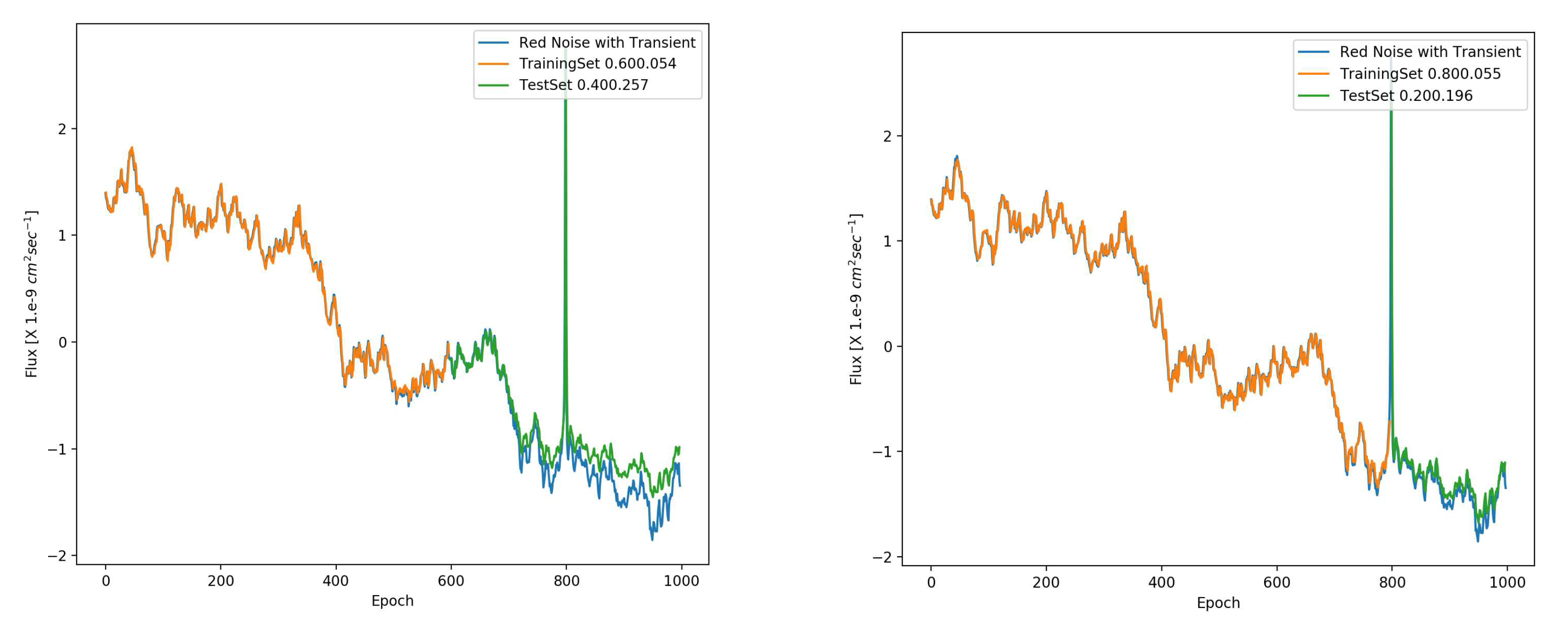
The results for the transient detection is shown in the Figure 14 and Figure 15 for pink and red noise respectively. We find that for pink noise, the prediction for the same transient is far superior to that for the red noise case. This is what we would expect from the simulation tests done in the previous sections. It is clear that the LSTMs perform rather poorly in presence of red noise and would give an imprecise prediction, not only for the transient, but in fact for the entire forecast. Now in absolute terms, one would expect the stateless LSTMs to fail at predicting a sharp, significant transient in either scenario, due to lack of long term correlation. However, given that there is a finite time, , and given the normalisation, we do find that the LSTMs have decent predictive power as a batch size of derives correlation on these timescales. And the closer we are to the outburst, the better the performance giving a very impressive value of loss (test to train) ratio of for an split for pink noise. This deteriorates to for a split.
6. Discussion and Conclusions
Sensitivity tests are critical for complex algorithms to test the stability of predictions and tendencies for certain types of datasets to yield certain types of results. Ever increasing volumes of time-domain data in astronomy at different wavelengths with CTA in gamma-rays [for eg., [1,2,3], SKA in radio [for eg., [4,5,6], LSST in optical [for eg., [7] has ushered in a new era in observational astronomy driven by data. This includes a variety of variable objects ranging from Galactic compact binaries and extragalactic sources like AGNs amd GBRs to the mysterious Fast Radio Bursts (FRBs). In this era, multi-wavelength campaigns will have to scale with the volumes of data with a high degree of automated and optimised or "intelligent" decision making, whether it is classification of transients or indeed follow-up observations. This will inevitably lead to a growing importance of the forecasting element. Hence exhaustive efforts are needed to test forecasting algorithms that are likely to be used. In this context, the RNN-LSTM models are likely to be a popular choice. Astronomical lightcurves, i.e. time-series generated by an astrophysical system are apriori expected to be less complex than those in other domains. However, the combination of interesting quasi-periodic signals and outbursts with interesting stochastic astrophysical signals and background noise, makes astronomical forecasting a non-trivial challenge. In several multiwavelength and now increasingly multimessenger observations, an episode of increased flux measured in one waveband by one telescope or observatory triggers other facilities in different wavebands to observe the same source position. This essentially comes from the idea that physical processes leaves imprints on different parts of the electromagnetic spectrum with time-lags. And coordinated or synchronous observations amongst other things aim at identifying and quantifying the driving physical processes in terms of observed lags. To facilitate these coordinated observations, precise, fast, and reliable forecasting is key, and here machine learning algorithms like the RNN LSTMs can be very useful. Therefore, it is worthwhile to test them against types of time-series that maybe encountered with simulated lightcurves.
In testing with simulated lightcurves, we perform two types of tests. The first is sensitivity to properties or characteristics of data. The second is sensitivity to elements of the forecasting machinery for different datasets. Under characteristics of data, we look at incompleteness in data, or gaps in lightcurves that we routinely encounter in astronomy observations. We simulate purely periodic and random gaps and vary the percentage of missing data points to compute the training and test losses as measures of performance. We find that red noise lightcurves are generally more affected by presence of both periodic and random gaps, than the pink noise. Another general outcome seems to be presence of a sweet spot for the fraction of gaps at around 20 or , where the test to train losses tend to be closest to unity and thereby optimal. One possible implication could be that the gaps could, to an extent reduce the complexity and thereby improve performance of a particular forecasting architecture. Another alternate scenario could be that as we move from pink to red noise i.e. from a power spectral density index of 1.0 to 2.0, the longer timescales are more significant than the shorter ones on which gaps are introduced. And this leads to an initial improvement with increase in gaps until, the extent of the gaps is large enough that eventually starts to hamper predictability. These two effects would be degenerate. A stronger conclusion would require a comparison with other machine learning algorithms or indeed other forecasting methods, which we leave for a future paper. The complexity measured in terms of no. of Fourier components has a more monotonic effect. As the number of Fourier components increase, the performance tends to deteriorate for both pink and red noise.
From the elements of the forecasting machinery or architecture, the most important one appears to be the batch size. Once again, there seems to be a sweet spot at a batch size of around 10 for performance in terms of both absolute values of losses and the ratio of test to train losses. The performance for a learning rate of 0.1 and train to test ratio of at first glance seems to be slightly better for red noise, with a hint of overfitting for pink noise with the test to train loss ratio dropping below 1.0 in some cases. This is shown in Figure 12. However this is not significant. What is more significant though is that this ratio and hence the performance is more stable for pink noise. This is confirmed by the uncertainty calculation in Figure 13 which shows a larger uncertainty for red noise. A possible, even likely reason for this is that for stateless mode in which we are operating the LSTMs, it does not account for correlations over longer timescales than within a batch. With greater power at longer timescales in red noise compared to pink noise, the LSTMs should have a worse performance. This should also imply that if stateful mode is used then the performance on the red noise lightcurves should improve more than that for the pink noise. Once again, there is a need to compare with other forecasting models which is beyond the scope of this paper and will be addressed in a future one. The main conclusions from this study are summarised below,
- Fast and precise, automated multiwavelength transient forecasting will become increasingly important to plan observational campaigns in the era of big astronomical data with multiple facilities such as SKA, LSST, CTA, etc. This is a natural application of multivariate forecasting with RNN-LSTMs. Hence studies of transients with methods of deep learning both methodological and astrophysical are of great relevance as has been echoed by others [eg., [11,12].
- Given a precedence of a transient or flare in historical or current lightcurves, we can predict statistically the occurrence of a flare in the future provided this is not a special episode unrelated to the parent distribution or process driving variability. This also suggests that the RNN-LSTMs could potentially be used to discriminate between flares from different distributions. This would require dedicated investigations which would be the subject of future papers.
- Deep learning methods in general are prone to overfitting in the presence of noise ; this is naturally a concern extending to applications beyond astrophysics (eg. financial predictions [40,41], meteorological forecasts [42]). This makes transient detection is therefore especially difficult. In astrophysics, flares are such transients can emerge from underlying astrophysical noise. Furthermore, quality of forecast depends upon the properties of this noise. For instance, we find that noise with steeper or "redder" power spectra makes transient detection less precise and more challenging. In other words, greater power and correlations on longer timescales will make it challenging to make good forecasts of flares. This is consistent with other challenges that accompany sources with steep power spectral densities. For instance, one would need to investigate direct effects of underlying distribution(s) and non-stationary behaviour of variations in sources with power spectral densities steeper than index of unity or flicker noise, [39] on these predictions. The response of the type of architecture to different types of noise especially with respect to overfitting deserves its own study and will be subject of future investigations.
- Univariate forecasting sensitivity in terms of the losses or scores depend upon complexity of data as well as the structure of neural network particularly batch size. The sensitivity to data characteristics varies in different ways. The losses increase monotonically with complexity measured in terms of no. of Fourier components. The sensitivity to incompleteness is less straightforward and depends on a number of aspects like the underlying distribution (PDF), and LSTM architecture and parameters (like activation) and noise properties (PSD). But in general, the sensitivity is greater for redder noise. There are multiple approaches to tackling missing data ; certain types of imputation can help for moderate MDF () [43]. Alternately one could encode the effects in terms of additional uncertainty (statistical) and bias (systematic) terms like we do for batch size. The dependence on the "structural parameters" of the network in general are not always straightforward or monotonic. This makes it challenging to come up with an optimal network in the most general case. However, from the current study we see that amongst the most crucial "structural parameters" is the batch size. For long term monitoring, a batch size of 10-30 gives good results. For other parts of the architecture, possible approaches are pre-training LSTM models with realistic simulations [eg., [38,39]. Yet another alternative is using historical data for this pre-training and this is feasible as forecasting systems can be tied to individual facilities at specific wavelengths.
The results show that in general, that while RNN LSTMs are powerful for forecasting time-series, there’s enough complexity and attention needs to be paid to selection of architecture parameters for different types of noise. This is vital for noisy time-series forecasting. Generative methods (or time-series simulations) can provide an excellent way of testing sensitivities to facilitate such selection and possibly pre-selection for forecasting algorithms to be deployed in actual observational astronomy campaigns. Clearly, the power spectral density and probability distribution function of lightcurves from past long-term campaigns are an incredibly useful guide in construction of forecasting machinery. Multiwavelength lightcurves will need multivariate forecasting. A deep dive into this will be the topic of a future paper.
Acknowledgments
NC kindly acknowledges the continued support from Coventry University, DARC, Reading and MPIK, Heidelberg for their resources used conduct this research.
Conflicts of Interest
The author declare no conflict of interest.
References
- Bartos, I.; Veres, P.; Nieto, D.; Connaughton, V.; Humensky, B.; Hurley, K.; Márka, S.; Mészáros, P.; Mukherjee, R.; O’Brien, P.; Osborne, J.P. Cherenkov Telescope Array is well suited to follow up gravitational-wave transients. MNRAS 2014, arXiv:astro-ph.HE/1403.6119]443, 738–749. [Google Scholar] [CrossRef]
- Bartos, I.; Di Girolamo, T.; Gair, J.R.; Hendry, M.; Heng, I.S.; Humensky, T.B.; Márka, S.; Márka, Z.; Messenger, C.; Mukherjee, R.; Nieto, D.; O’Brien, P.; Santander, M. Strategies for the follow-up of gravitational wave transients with the Cherenkov Telescope Array. MNRAS 2018, arXiv:astro-ph.HE/1802.00446]477, 639–647. [Google Scholar] [CrossRef]
- Schüssler, F. The Transient program of the Cherenkov Telescope Array. 36th International Cosmic Ray Conference (ICRC2019), 2019, Vol. 36, International Cosmic Ray Conference, p. 788, [arXiv:astro-ph.HE/1907.07567]. arXiv:astro-ph.HE/1907.07567].
- Fender, R.; Stewart, A.; Macquart, J.P.; Donnarumma, I.; Murphy, T.; Deller, A.; Paragi, Z.; Chatterjee, S. The Transient Universe with the Square Kilometre Array. Advancing Astrophysics with the Square Kilometre Array (AASKA14), 2015, p. 51, [arXiv:astro-ph.HE/1507.00729]. arXiv:astro-ph.HE/1507.00729].
- Macquart, J.P.; Keane, E.; Grainge, K.; McQuinn, M.; Fender, R.; Hessels, J.; Deller, A.; Bhat, R.; Breton, R.; Chatterjee, S.; Law, C.; Lorimer, D.; Ofek, E.O.; Pietka, M.; Spitler, L.; Stappers, B.; Trott, C. Fast Transients at Cosmological Distances with the SKA. Advancing Astrophysics with the Square Kilometre Array (AASKA14), 2015, p. 55, [arXiv:astro-ph.HE/1501.07535]. arXiv:astro-ph.HE/1501.07535].
- Banyer, J.; Murphy, T.; VAST Collaboration., VAST: A Real-time Pipeline for Detecting Radio Transients and Variables on the Australian SKA Pathfinder (ASKAP) Telescope. In Astronomical Data Analysis Software and Systems XXI. Proceedings of a Conference held at Marriott Rive Gauche Conference Center, Paris, France, 6-10 November, 2011. ASP Conference Series, Vol. 461. Edited by P. Ballester, D. Egret, and N.P.F. Lorente. San Francisco: Astronomical Society of the Pacific, 2012., p.725; Ballester, P.; Egret, D.; Lorente, N.P.F., Eds.; 2012; Vol. 461, Astronomical Society of the Pacific Conference Series, p. 725.
- Borne, K.D. A machine learning classification broker for the LSST transient database. Astronomische Nachrichten 2008, 329, 255. [Google Scholar] [CrossRef]
- Bloom, J.S.; Richards, J.W.; Nugent, P.E.; Quimby, R.M.; Kasliwal, M.M.; Starr, D.L.; Poznanski, D.; Ofek, E.O.; Cenko, S.B.; Butler, N.R.; Kulkarni, S.R.; Gal-Yam, A.; Law, N. Automating Discovery and Classification of Transients and Variable Stars in the Synoptic Survey Era. PASP 2012, arXiv:astro-ph.IM/1106.5491]124, 1175. [Google Scholar] [CrossRef]
- Hinners, T.A.; Tat, K.; Thorp, R. Machine Learning Techniques for Stellar Light Curve Classification. AJ 2018, arXiv:astro-ph.IM/1710.06804]156, 7. [Google Scholar] [CrossRef]
- Faisst, A.L.; Prakash, A.; Capak, P.L.; Lee, B. How to Find Variable Active Galactic Nuclei with Machine Learning. ApJL 2019, arXiv:astro-ph.IM/1908.07542]881, L9. [Google Scholar] [CrossRef]
- Muthukrishna, D.; Narayan, G.; Mandel, K.S.; Biswas, R.; Hložek, R. RAPID: Early Classification of Explosive Transients Using Deep Learning. PASP 2019, arXiv:astro-ph.IM/1904.00014]131, 118002. [Google Scholar] [CrossRef]
- Sadeh, I. Deep learning detection of transients (ICRC-2019). arXiv e-prints 2019, p. arXiv:1908.01615, [arXiv:astro-ph.HE/1908.01615]. arXiv:1908.01615, [arXiv:astro-ph.HE/1908.01615].
- Khouider, B.; Majda, A.J.; Katsoulakis, M.A. Coarse-grained stochastic models for tropical convection and climate. Proceedings of the National Academy of Sciences 2003, 100, 11941–11946, [https://www.pnas.org/doi/pdf/10.1073/pnas.1634951100].. [Google Scholar] [CrossRef]
- Reichle, R.H. Data assimilation methods in the Earth sciences. Advances in Water Resources 2008, 31, 1411–1418, Hydrologic Remote Sensing. [Google Scholar] [CrossRef]
- Kim, S.; Kang, M. Financial series prediction using Attention LSTM. arXiv e-prints 2019, p. arXiv:1902.10877, [arXiv:cs.LG/1902.10877]. arXiv:1902.10877, [arXiv:cs.LG/1902.10877].
- Bui, T.C.; Le, V.D.; Cha, S.K. A Deep Learning Approach for Forecasting Air Pollution in South Korea Using LSTM. arXiv e-prints 2018, p, arXiv:1804.07891, [arXiv:cs.LG/1804.07891].
- Lee Giles, C.; Lawrence, S. Noisy Time Series Prediction using Recurrent Neural Networks and Grammatical Inference. Machine Learning 2001, 44, 161–183. [Google Scholar] [CrossRef]
- Goodfellow, I.; Bengio, Y.; Courville, A. Deep Learning; MIT Press, 2016. http://www.deeplearningbook.org.
- Djorgovski, S.G.; Mahabal, A.A.; Donalek, C.; Graham, M.J.; Drake, A.J.; Moghaddam, B.; Turmon, M. Flashes in a Star Stream: Automated Classification of Astronomical Transient Events. arXiv e-prints 2012, p. arXiv:1209.1681, [arXiv:astro-ph.IM/1209.1681].
- Chatfield, C.; Yar, M. Holt-Winters Forecasting: Some Practical Issues. The Statistician 1988, 37. [Google Scholar] [CrossRef]
- Siami-Namini, S.; Siami Namin, A. Forecasting Economics and Financial Time Series: ARIMA vs. LSTM. arXiv e-prints 2018, p. arXiv:1803.06386, [arXiv:cs.LG/1803.06386].
- Nelson, D.B. Conditional Heteroskedasticity in Asset Returns: A New Approach. Econometrica 1991, 59, 347–370. [Google Scholar] [CrossRef]
- Breiman, L. Random Forests. Machine Learning 2001, 45, 5–32. [Google Scholar] [CrossRef]
- Friedman, J.H. Greedy function approximation: A gradient boosting machine. Ann. Statist. 2001, 29, 1189–1232. [Google Scholar] [CrossRef]
- Hochreiter, S.; Schmidhuber, J. Long short-term memory. Neural computation 1997, 9, 1735–1780. [Google Scholar] [CrossRef]
- Greff, K.; Srivastava, R.K.; Koutník, J.; Steunebrink, B.R.; Schmidhuber, J. LSTM: A Search Space Odyssey. arXiv e-prints 2015, p. arXiv:1503.04069, [arXiv:cs.NE/1503.04069].
- Dorner, D.; Ahnen, M.L.; Bergmann, M.; Biland, A.; Balbo, M.; Bretz, T.; Buss, J.; Einecke, S.; Freiwald, J.; Hempfling, C.; Hildebrand, D.; Hughes, G.; Lustermann, W.; Mannheim, K.; Meier, K.; Mueller, S.; Neise, D.; Neronov, A.; Overkemping, A.K.; Paravac, A.; Pauss, F.; Rhode, W.; Steinbring, T.; Temme, F.; Thaele, J.; Toscano, S.; Vogler, P.; Walter, R.; Wilbert, A. FACT - Monitoring Blazars at Very High Energies. arXiv e-prints 2015, p. arXiv:1502.02582, [arXiv:astro-ph.IM/1502.02582].
- Schüssler, F.; Seglar-Arroyo, M.; Arrieta, M.; Böttcher, M.; Boisson, C.; Cerruti, M.; Chakraborty, N.; Davids, I.D.; Felix, J.; Lenain, J.P.; Prokoph, H.; Sanchez, D.; Wagner, S.; Zacharias, M.; Zech, A.; H. E. S. S. Collaboration. Target of Opportunity Observations of Blazars with H.E.S.S. 35th International Cosmic Ray Conference (ICRC2017), 2017, Vol. 301, International Cosmic Ray Conference, p. 652, [arXiv:astro-ph.HE/1708.01083].
- Blinov, D.; Pavlidou, V. The RoboPol Program: Optical Polarimetric Monitoring of Blazars. Galaxies 2019, arXiv:astro-ph.HE/1904.05223]7, 46. [Google Scholar] [CrossRef]
- Namini, S.S.; Tavakoli, N.; Namin, A.S. A Comparison of ARIMA and LSTM in Forecasting Time Series. 2018, pp. 1394–1401. [CrossRef]
- Han, J.H. Comparing Models for Time Series Analysis. Applied Statistics Commons and Statistical Models Commons, Wharton Research Scholars 2018, p. 162.
- Lai, G.; Chang, W.; Yang, Y.; Liu, H. Modeling Long- and Short-Term Temporal Patterns with Deep Neural Networks. CoRR 2017, abs/1703.07015, [1703.07015].
- Lipton, Z.C. The Mythos of Model Interpretability. arXiv e-prints 2016, p. arXiv:1606.03490, [arXiv:cs.LG/1606.03490]. arXiv:1606.03490, [arXiv:cs.LG/1606.03490].
- Doshi-Velez, F.; Kim, B. Towards A Rigorous Science of Interpretable Machine Learning. arXiv e-prints 2017, p. arXiv:1702.08608, [arXiv:stat.ML/1702.08608].
- Timmer, J.; Koenig, M. On generating power law noise. AAP 1995, 300, 707. [Google Scholar]
- Emmanoulopoulos, D.; McHardy, I.M.; Papadakis, I.E. Generating artificial light curves: revisited and updated. MNRAS 2013, arXiv:astro-ph.IM/1305.0304]433, 907–927. [Google Scholar] [CrossRef]
- Romoli, C.; Chakraborty, N.; Dorner, D.; Taylor, A.; Blank, M. Flux Distribution of Gamma-Ray Emission in Blazars: The Example of Mrk 501. Galaxies 2018, arXiv:astro-ph.HE/1812.06204]6, 135. [Google Scholar] [CrossRef]
- Chakraborty, N. Investigating Multiwavelength Lognormality with Simulations : Case of Mrk 421. arXiv e-prints 2020, p. arXiv:2001.02458, [arXiv:astro-ph.HE/2001.02458]. arXiv:2001.02458, [arXiv:astro-ph.HE/2001.02458].
- Morris, P.J.; Chakraborty, N.; Cotter, G. Deviations from normal distributions in artificial and real time series: a false positive prescription. MNRAS 2019, arXiv:astro-ph.HE/1908.04135]489, 2117–2129. [Google Scholar] [CrossRef]
- Lu, C.J.; Lee, T.S.; Chiu, C.C. Financial time series forecasting using independent component analysis and support vector regression. Decision Support Systems 2009, 47, 115–125. [Google Scholar] [CrossRef]
- Tang, Q.; Fan, T.; Shi, R.; Huang, J.; Ma, Y. Prediction of financial time series using LSTM and data denoising methods, 2021, [arXiv:econ.EM/2103.03505]. arXiv:econ.EM/2103.03505].
- Karevan, Z.; Suykens, J.A. Transductive LSTM for time-series prediction: An application to weather forecasting. Neural Networks 2020, 125, 1–9. [Google Scholar] [CrossRef]
- Che, Z.; Purushotham, S.; Cho, K.; Sontag, D.; Liu, Y. Recurrent Neural Networks for Multivariate Time Series with Missing Values. Scientific Reports 2016, 8. [Google Scholar] [CrossRef]
| 1 | |
| 2 | |
| 3 | |
| 4 | |
| 5 | |
| 6 | |
| 7 |
Figure 1.
The figure shows the basic structure of an RNN-LSTM block within a segment of the network with the time axes unrolled. The output from the previous block, is combined optimally with input, at the current stage, to produce output at this stage. represents the "forget gate" that determines if the previous internal state, , which is a combination of and is passed through or forgotten. The input gate, determines the internal state at the current stage, and the output gate, determines how much of this current state is passed on to the output.
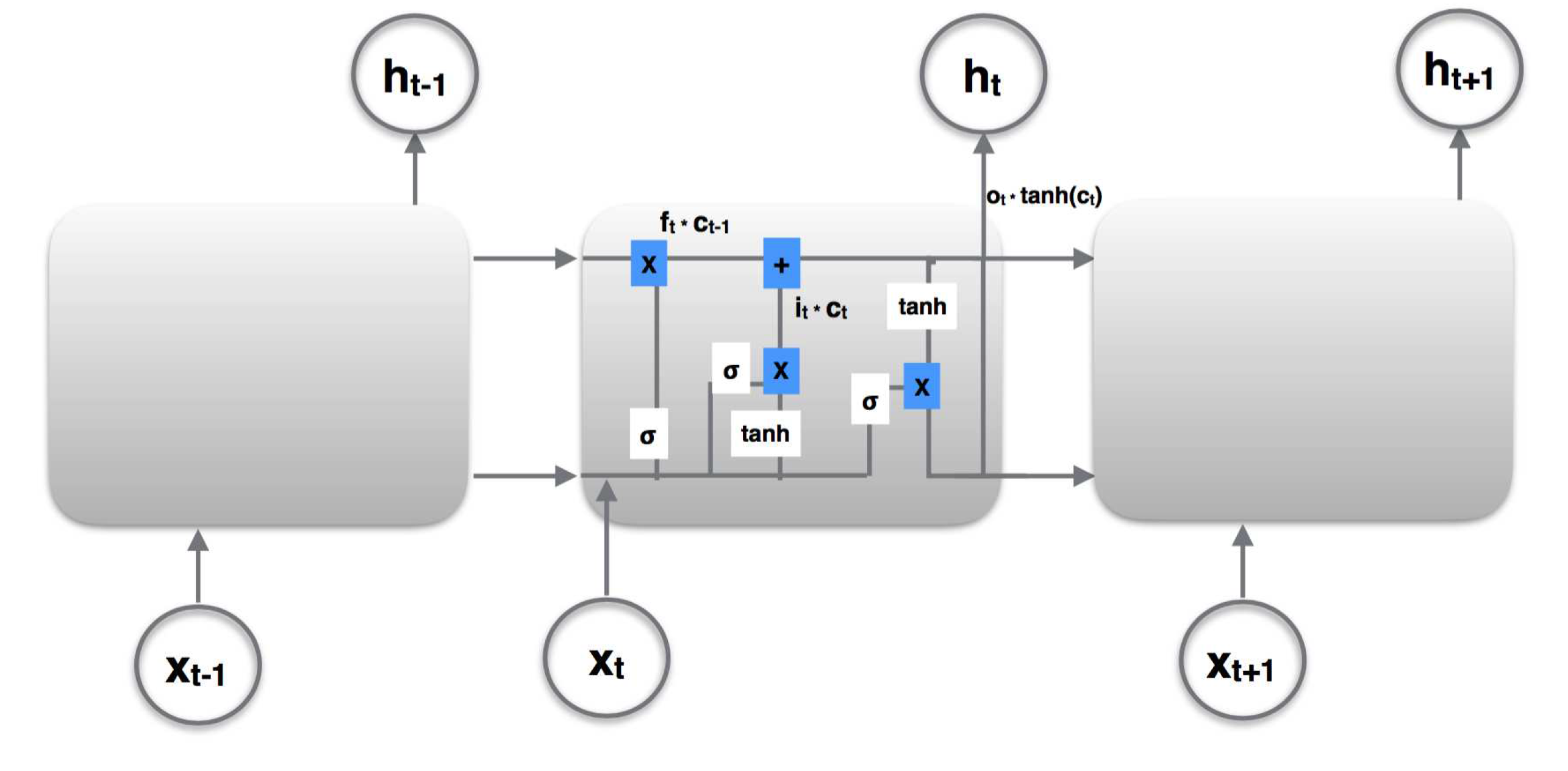
Figure 2.
The figure shows the basic structure of an RNN network structure. Essentially it is composed of an input and output layers comprising of blocks representing the input and output data. In between there are one or more hidden layers consisting of the blocks, which perform the actual "fitting of the model".
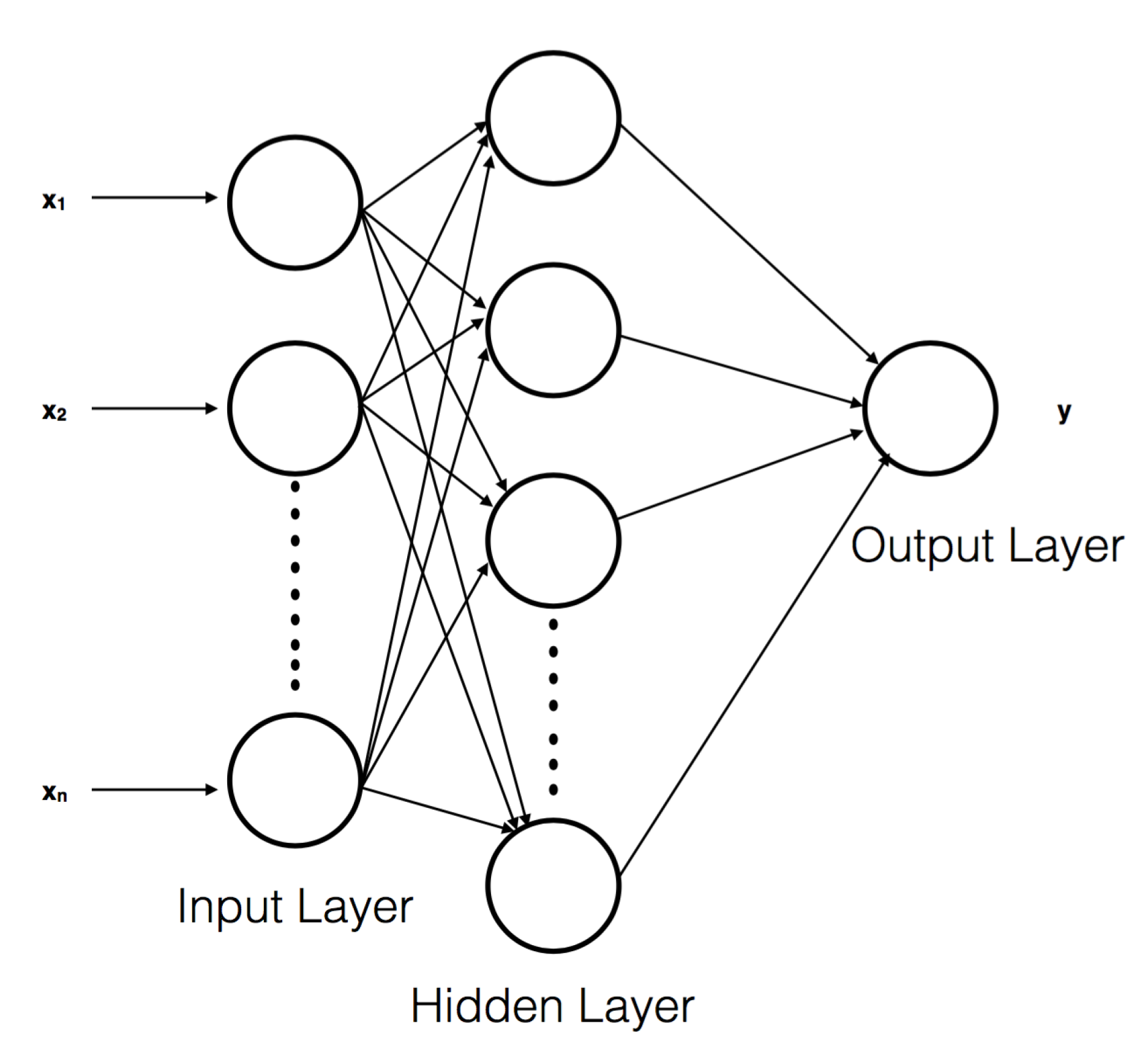
Figure 3.
The figure shows an example of multivariate forecasting with RNN-LSTM. Here two input lightcurves one purely red noise (green) and the other red noise plus transient (blue) are used to predict a flare in a third lightcurve (orange). These lightcurves are artificially generated and scaled in amplitude for presentation purposes. It is clear that if the training data has flare-like features similar to ones we wish to forecast, then we could predict such flares in test data or future lightcurves.
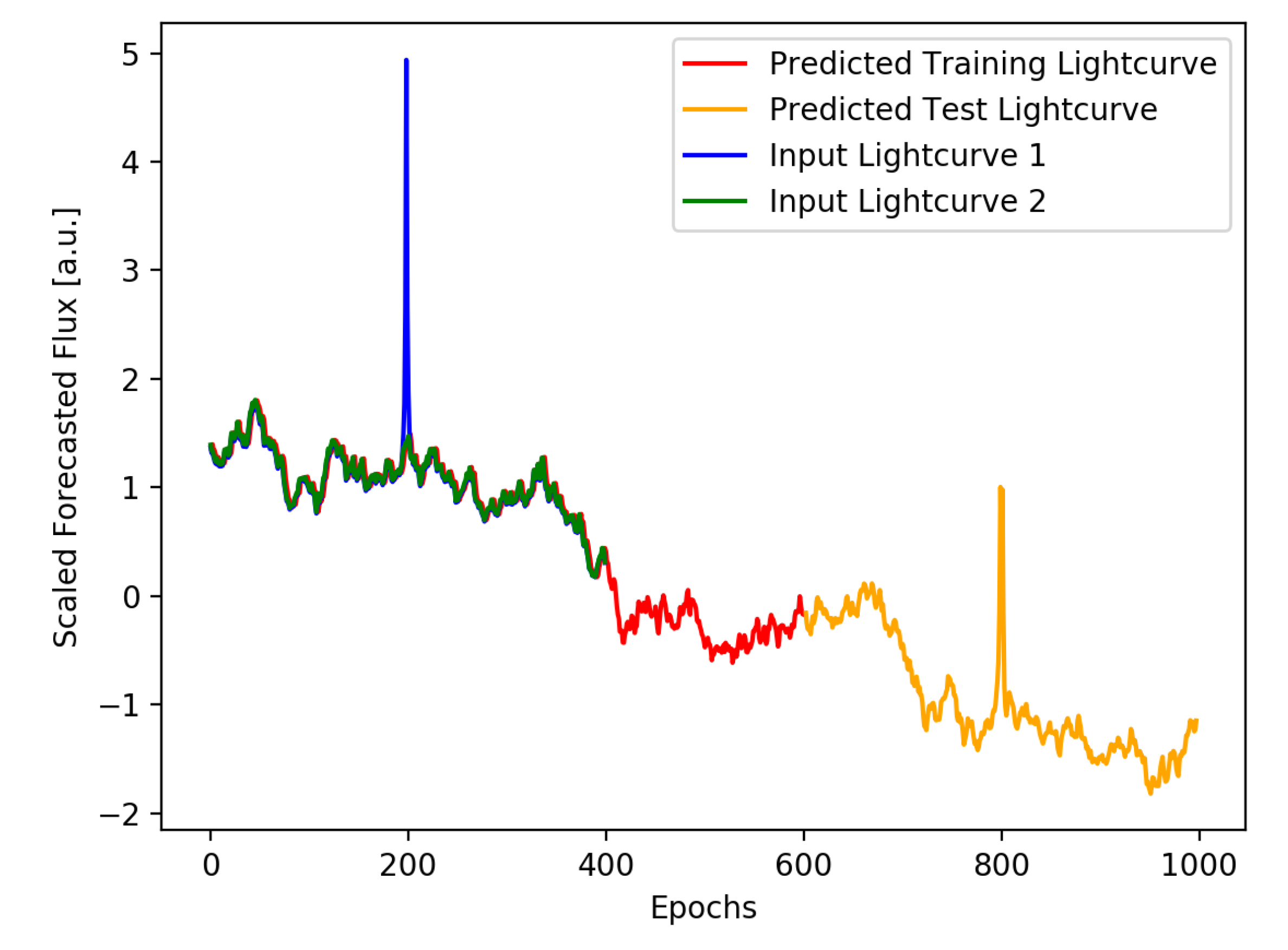
Figure 4.
Top: The figure shows the prediction of a strictly periodic signal with a period of a year, with RNNs with LSTM. This is a trivial case of forecasting for a time-series exactly known.Center and Bottom: The signal is once again the annual periodicity, but with missing data. In each of these cases, the proportion of the size of test to train dataset is given adjacent to the score. As shown, this affects the prediction a small amount.
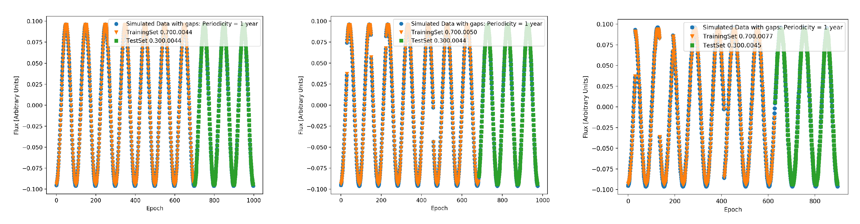
Figure 5.
Top: The figure shows the prediction of the annual periodic signal modulating a stochastic, pink noise signal, with RNNs with LSTM. The prediction while not trivial as the strictly periodic case, is still strong. Center: The same signal with missing data () clearly makes trickier to predict accurately. Bottom: With of missing data seems to be exactly precise yet this is misleading.
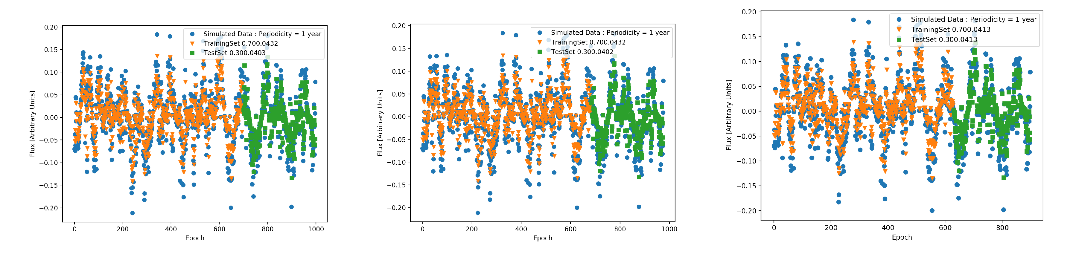
Figure 6.
The ratio of the test to train loss is shown as a function of the percentage of periodic gaps in data for pink (blue and red noise (red). This is shown for hard sigmoid (solid) and tanh (dashed) activation with the latter as the most optimal scenario. For fraction of gaps exceeding , the accuracy gets worse as proportion of missing data increases. This deterioration is less pronounced for pink noise.
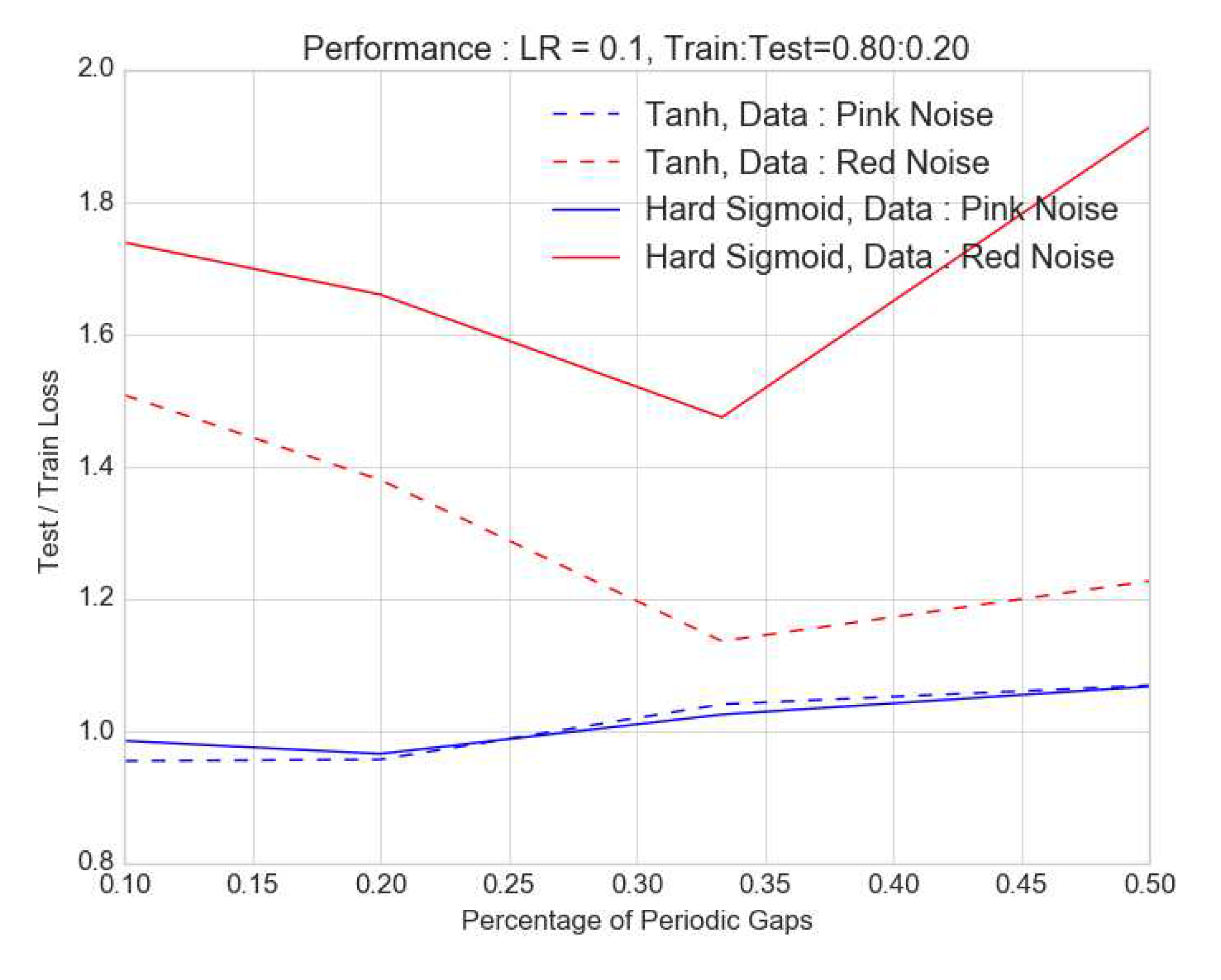
Figure 7.
Like in Figure 3, the ratio of the test to train loss is shown as a function of the percentage of random gaps in data for pink (blue and red noise (red) ; once again the activation functions are hard sigmoid (solid) and tanh (dashed). For fraction of gaps exceeding , the accuracy gets worse as proportion of missing data increases. This deterioration is less pronounced for pink noise.
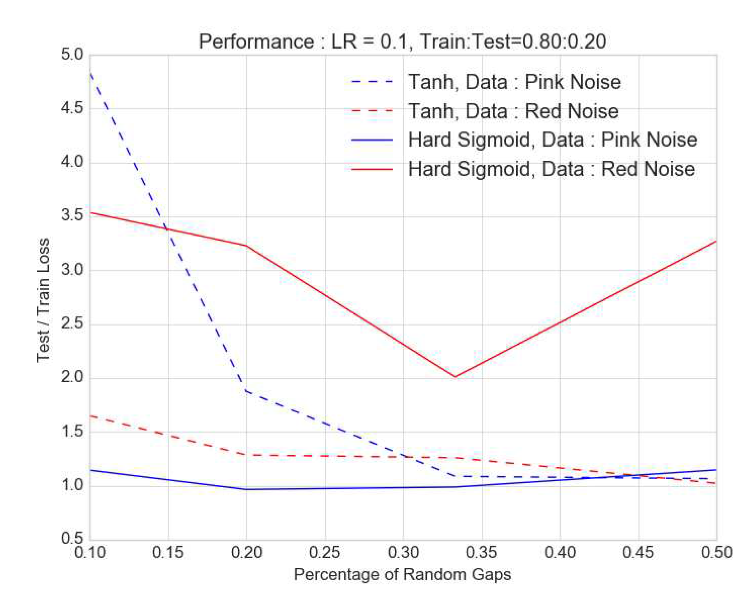
Figure 8.
The test (blue) and train (red) losses are shown as a function of the no. of Fourier components in the pink noise signal ; the activation functions are hard sigmoid (solid) and tanh (dashed). As the complexity i.e. the number of Fourier components increase, both the train and test losses increase as predictions tend to get harder to make.
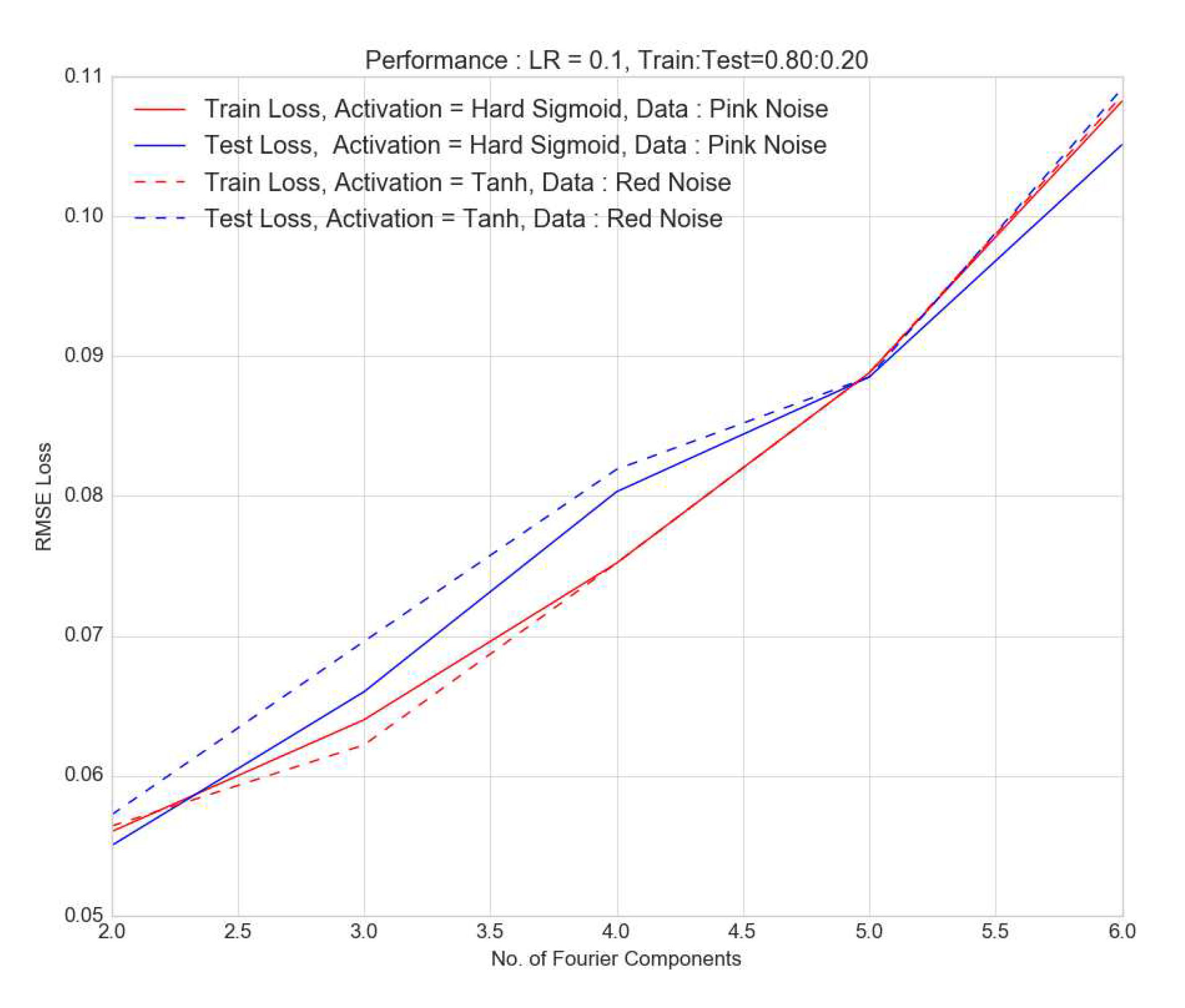
Figure 9.
The ratio of test to train loss as function of lookback is shown for the pink noise case. It shows that the train and test loss values are the closest with the ratio being nearest to 1 for lookback of 10.
Figure 9.
The ratio of test to train loss as function of lookback is shown for the pink noise case. It shows that the train and test loss values are the closest with the ratio being nearest to 1 for lookback of 10.
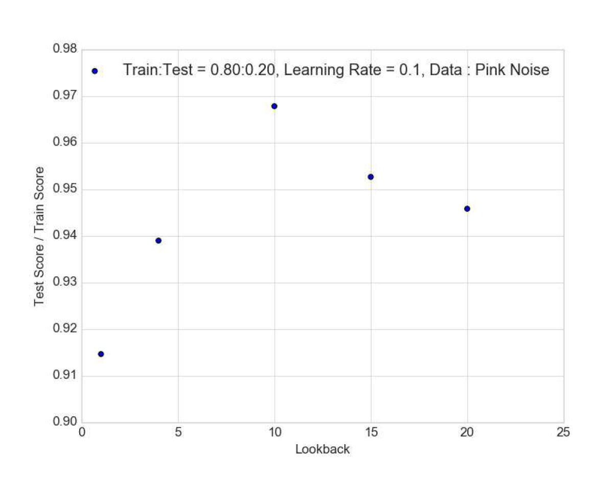
Figure 10.
The dependence of RMSE loss of pink (Left) and red (Right) noise process on the layers is shown in the figure for a learning rate of 0.1 and a train to test ratio of . While there is sensitivity to the number of identical RNN-LSTM layers, there is neither a trend nor a "sweet spot" for this number. This is suggestive that adding layers does not improve performance dramatically. In general, the performance is better or more consistent for pink noise.
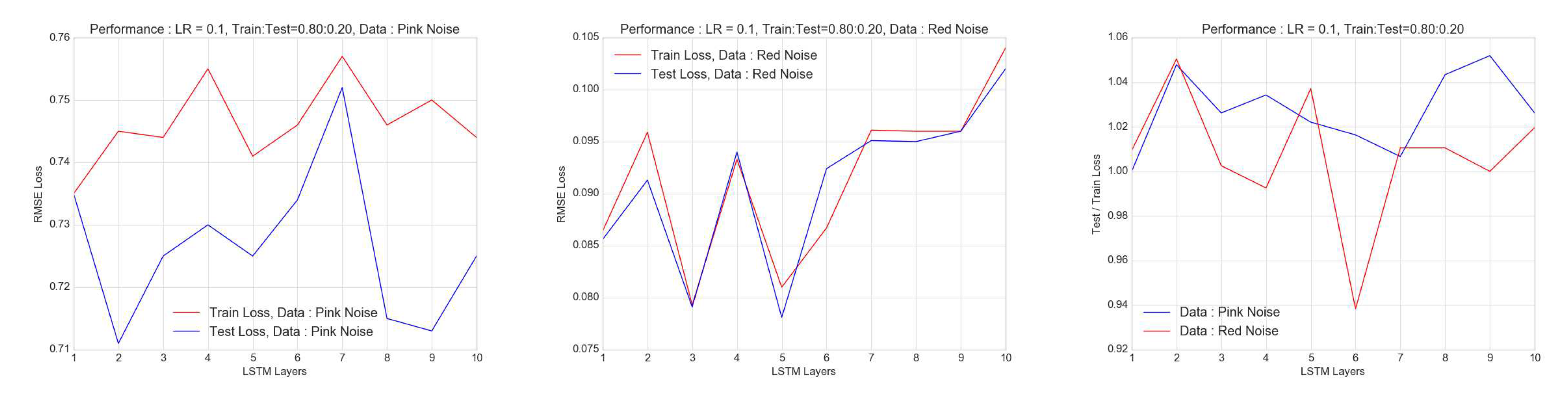
Figure 11.
The dependence of prediction accuracy of the pink noise process on the learning rate is shown in the figure for a batch size of 1 and a train to test ratio of . The learning rate does not impact the test and train scores significantly just the rate of convergence.
Figure 11.
The dependence of prediction accuracy of the pink noise process on the learning rate is shown in the figure for a batch size of 1 and a train to test ratio of . The learning rate does not impact the test and train scores significantly just the rate of convergence.
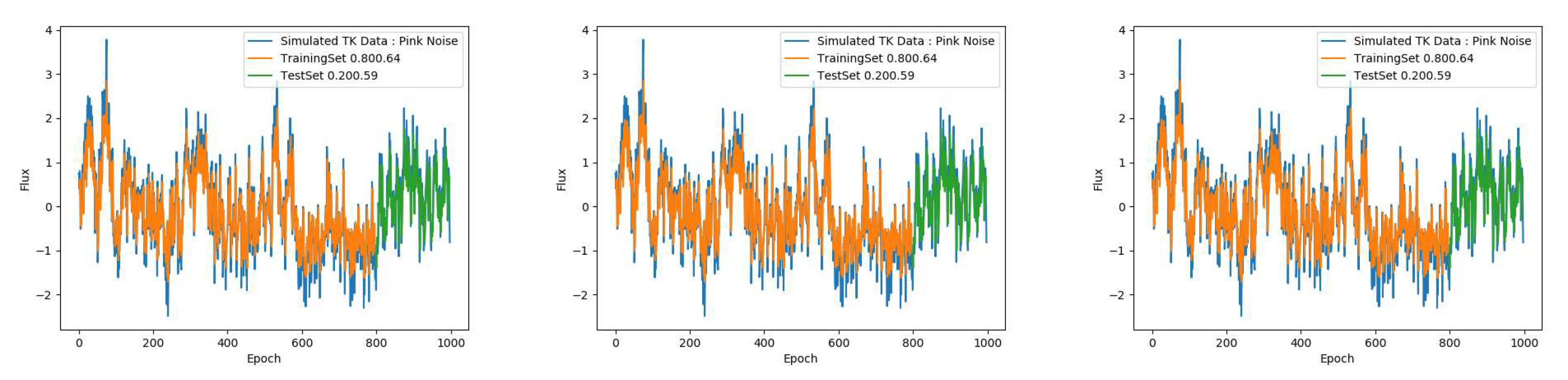
Figure 12.
The dependence of training and test losses of the pink and red noise processes on the batch size is shown in the figure for a train to test ratio of .
Figure 12.
The dependence of training and test losses of the pink and red noise processes on the batch size is shown in the figure for a train to test ratio of .
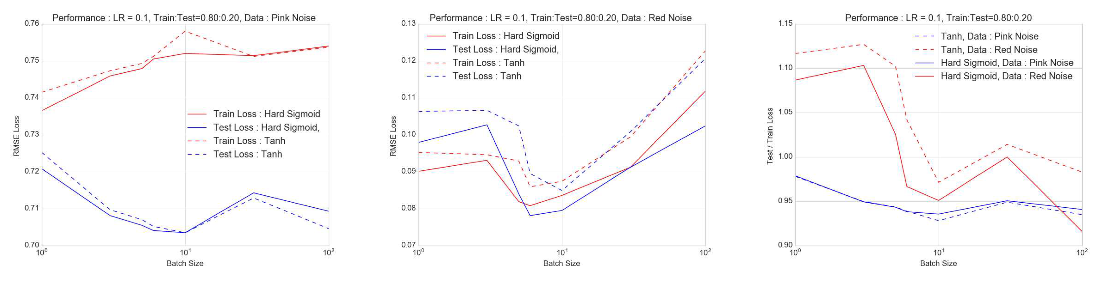
Figure 13.
The uncertainty on the effect of batch size is calculated by repeating the exercise in Figure 12 over 100 simulations of pink and red noise. Uncertainty on test loss is shown in blue, whereas that on the training loss is shown in red. This shows an optimal batch size of with a hint of overfitting with pink noise.
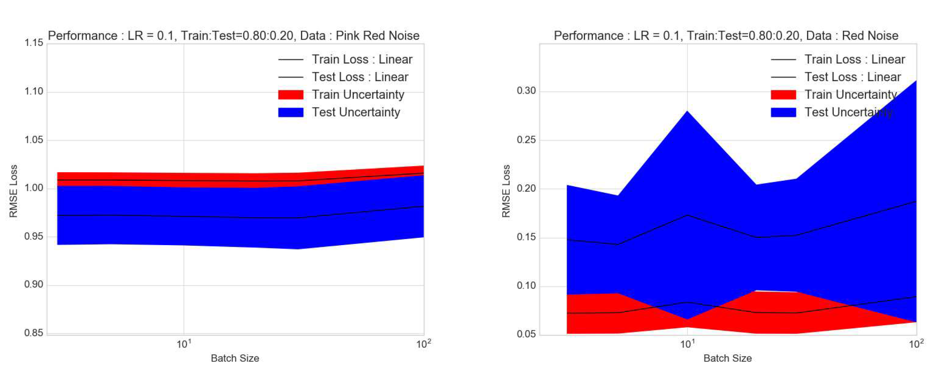
Figure 14.
The figure shows detection of a transient in presence of pink noise. To the left, is a train to test split of and to the right is a split. The LSTM with batch size 30 performs well, improving as we go nearer to the exponentially shaped transient.
Figure 14.
The figure shows detection of a transient in presence of pink noise. To the left, is a train to test split of and to the right is a split. The LSTM with batch size 30 performs well, improving as we go nearer to the exponentially shaped transient.
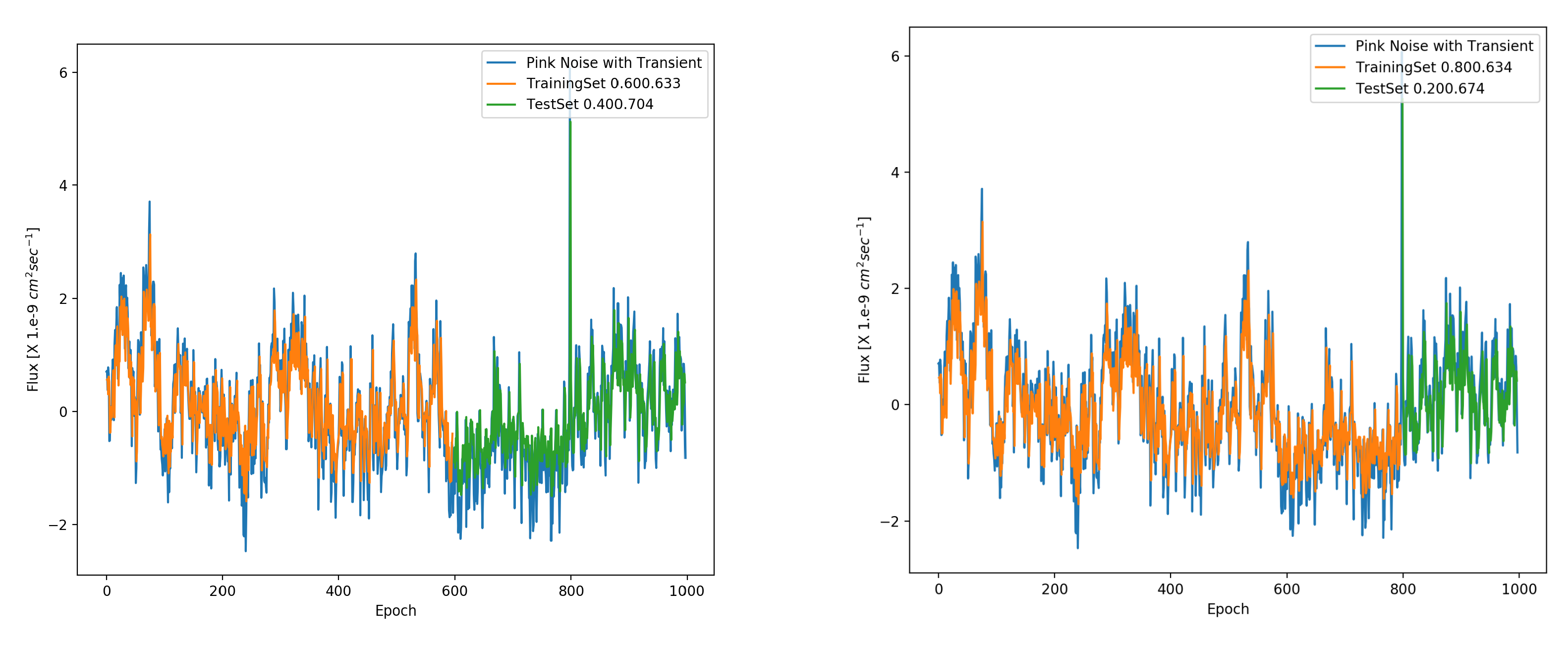
Figure 15.
Same as Figure 14 but with red noise. The LSTM with batch size 30 performs rather poorly showing the effect of noise.
Figure 15.
Same as Figure 14 but with red noise. The LSTM with batch size 30 performs rather poorly showing the effect of noise.
Disclaimer/Publisher’s Note: The statements, opinions and data contained in all publications are solely those of the individual author(s) and contributor(s) and not of MDPI and/or the editor(s). MDPI and/or the editor(s) disclaim responsibility for any injury to people or property resulting from any ideas, methods, instructions or products referred to in the content. |
© 2023 by the authors. Licensee MDPI, Basel, Switzerland. This article is an open access article distributed under the terms and conditions of the Creative Commons Attribution (CC BY) license (http://creativecommons.org/licenses/by/4.0/).
Copyright: This open access article is published under a Creative Commons CC BY 4.0 license, which permit the free download, distribution, and reuse, provided that the author and preprint are cited in any reuse.


