
You are currently viewing a beta version of our website. If you spot anything unusual, kindly let us know.
Preprint
Article
The Solar System: Nature and Mechanics
Altmetrics
Downloads
1202
Views
1198
Comments
1


This version is not peer-reviewed
Abstract
Origin, mechanics and properties of the Solar System are analysed in the framework of the Complete Relativity theory (by the same author). According to Complete Relativity, everything is relative. Any apparent absolutism (notably invariance to scale of dimensional constants, absolute elementariness, invariance to time) is an illusion stemming from limits imposed by [or on] polarized observers that will inevitably lead to misinterpretation of phenomena (another illusion) occurring on non-directly observable scales or even on observable but distant scales in space or time. If everything is relative, reference frames will exist where particles are planets and where planets are living beings. Earth is, therefore, analysed here in more detail, both as a particle and, as a living evolving being (of, hypothesized, extremely introverted intelligence). The analysis confirms the postulates and hypotheses of the theory (ie. existence of discrete vertical energy levels) with a significant degree of confidence. During the analysis, some new hypotheses have emerged. These are discussed and confirmed with various degrees of confidence. To increase confidence or refute some hypotheses, experimental verification is necessary. Main conclusions that stem from my research and are further confirmed in this paper are: universes are, indeed, completely relative; Solar System is a scaled (inflated, in some interpretations) Carbon isotope with a nucleus in a condensed (bosonic) state and components in various vertically excited states; life is common everywhere, albeit extroverted complex forms are present on planetary surfaces only during planetary neurogenesis; anthropogenic climate change is only a part (trigger from one perspective) of bigger global changes; major extinction events on a surface of a planet are relative extinctions, a regular part of transformation and transfer of life in the process of planetary neurogenesis.
Keywords:
Subject: Physical Sciences - Astronomy and Astrophysics
1. Introduction
Here I hypothesize that the Solar System is either a large scale C atom (10-Carbon isotope) or a superposition of such atoms in a relatively special state and provide evidence for the equivalence of large (U) scale systems with standard (U) scale systems through the analysis of the Solar System in the context of Complete Relativity[1] (CR).
I hypothesize that structure of planetary systems is a result of inflation of gravitational maxima from standard scale atoms, likely in the events of annihilation at relative event horizons (gravitational maxima) of a particular scale.
I propose that, in this process, the electro-magnetic component of the general force has been exchanged with the neutral gravitational component resulting in the dominance of gravity over electro-magnetic force at this scale.
However, I also propose that such exchange is natural on standard scale - atoms are cycling between polarized and neutral states (although durations in particular states might be inverted between scales).
In any case, the hypothesized equivalence between the Solar System and the C atom should be taken relative.
Implications of discrete vertical energy levels [and CR in general] on nature are large and particularly affect the understanding of life. Existence of these levels is required for conservation of relativity but one consequence is relativization of components of living beings (ie. living tissue, blood, etc.) between scales - they operate on different timescales and generally have different composition. In example, standard blood (blood of U scale), scaled to U scale will not be the same substance simply containing zillion extra standard cells, rather, to an U scale observer it will appear much different. Indeed, what I will consider the blood of a planet is commonly interpreted as magma. Thus, the planets can be living beings and here I will analyse Earth not only as a particle but as an evolving living being.
2. Constants
Table 1 shows commonly used constants in the paper.
The values of planetary constants are taken from NASA Planetary Fact Sheet[2].
3. Definitions
Definitions of terms and expressions that may be used in the paper. Note that these may be different than standard or common definitions in everyday use.
Some terms in use in this paper have been defined in CR and reader should be familiar with these (and CR in general) if the aim is to understand this paper properly.
3.1. Elementary charge
Elementary particles, relative to a universe of a particular scale, are generally polarized.
Physical interpretation (manifestation) of polarization is dependable on environment, but any elementary particle can be interpreted as a more or less evolved graviton (as defined in CR).
In case its electro-magnetic component is dominant, the particle is electrically charged and represents a relative electric monopole.
However, electric component is generally a sum of multiple constituent charge quanta, typically 2 quanta of identical charge and 1 quantum of opposite (anti) charge, which are strongly entangled (there are no absolute monopoles). Spin momentum of charge is quantized, by a relative constant (ℏ) - a quantum of momentum.
Suppose the spin momentum of each is equal to 1/2 ℏ in value, and spins of two dominant charges are perpendicular to each other (having a [fixed] phase difference of /2 degrees). Two dominant charges now have a total magnetic spin momentum:
Total spin momentum of the particle is thus:
If the S (anti) charge momentum is perpendicular to S, the value of total spin momentum is:
Due to fixed /2 phase and equal value, influence of components of S on the orientation [of the momentum projection] cancel (the two components are fermions in the same quantum energy level, so their projections cannot both be oriented in the same direction), and the orientation of the projection of the momentum S on the axis of quantization will depend solely on the orientation of momentum S.

With the applied magnetic field, projection of the momentum on the magnetic axis (ie. z) will thus be oriented either up or down:
This is a typical spin momentum of standard charges such as electrons and protons.
Figure 1 a) shows charge in a collapsed state (as a particle) with acquired (coupled) real mass m, charge radii r, r (corresponding to momenta S and S, respectively) and radius of imaginary mass r, here having a momentum aligned with S.
Its momentum is quantized by ℏ, electric charge by e and gravitational force by . The private space of such particle may be, depending on a reference frame, characterized either by properly scaled gradients or averages, of electric permittivity () and magnetic permeability () - or pressure and density.
With a decrease in environmental pressure (em/gravitational field interactions) a quantum may split into smaller quanta (which remain strongly entangled), spreading as far as possible (the range is finite and determined by the mass of smaller quanta - or environmental pressure on that scale), with a wave-like distribution of potential. Figure 2 illustrates such relatively unbound, free charge. Total momentum is the sum of individual momenta (and equal to original momentum of the particle in case of isotropic effect). With the splitting, the quantum of energy will decouple from real mass m unless the splitting is synchronized with the dilution or explosion of mass m where individual quanta of m are of appropriate scale and momenta to couple with individual quanta of img mass.
Figure 3 a) shows one interpretation of strength of forces of a wave with distance from centre (black = gravitational force, blue and red = electric force). Now each component (maximum) of a wave, starting from outer ones, can be excited independently, can change spin, merge with adjacent maxima and form moon charges.
This allows the charge to interact (interfere) with itself in certain reference frames.
However, if components are strongly entangled in a particular reference frame, entanglement will be conserved with any interaction - the waveform may simply collapse (localize) into corpuscular form.
Figure 3 b) shows how the private space of the same particle can be modified by interaction with another particle - essentially, the electric force has been exchanged for gravitational force. Such interaction may also collapse the wave into a particle with moon charges, where the number of moons depends on the equilibrium point of interaction (difference in energy of interacting particles).
Note that it is possible for the effect to be strongly localized - local space may be modified to attenuate one force and strengthen the other, while particles outside that space may not feel such [degree of] change.
3.1.1. Equilibrium and nature of forces
Equilibrium state of 3 components of charge is maintained through angular momenta. Due to rotation of local space, general force is a centripetal force and in stable orbitals equal to centrifugal force.
In case of a completely neutral (gravitational) force:
This is established when angular velocity of the orbiting body and angular velocity of space (effective graviton, or gravitational field tube) become equal:
If the body increases velocity (v > v), centrifugal force becomes greater than gravitational force and now acts as a fictitious repulsive force.
For v < v, gravitational force is higher than centrifugal force, and the body feels attractive force.
Nature (polarization) of the force can thus be changed with a change in radii (expansion/collapse) of gravitational maxima.
This allows for electro-magnetic force to be a fictitious force - a result of radii change of gravitational maxima due to absorption and emission of energy.
Even if orbital changes are not electro-magnetic in nature, such changes imply radial polarization of reference frames, thus a reference frame can be polarized even if its mass is purely gravitational, and this will be reflected in a relativistic () factor.
However, there are no absolutely pure gravitational reference frames and changes in stable orbits may generally happen with the exchange of gravitational for electro-magnetic potential.
In that case, gravitational polarization becomes electric polarization.
3.2. Primary atom radius
Generally, radius of an atom is assumed to be equal to the radius of its outermost electron orbit.
However, other particles can be bound to atomic nuclei. Here, I hypothesize that neutrinos and anti-neutrinos are standardly bound to nuclei, generally occupying separate energy levels but may also be bound to other particles (ie. forming an electron/neutrino pair).
Primary radius of the atom is then equal to the orbital radius of its outermost primary component.
At minimum, it is equal to the general (outermost electron orbit) radius of the atom. However, at equilibrium - with all primary neutrinos present, it may be over twice that radius.
Here, a bound particle is considered primary if it is a component of the system equilibrium state (this is further discussed in chapter Initial structure hypothesis).
3.3. MAU
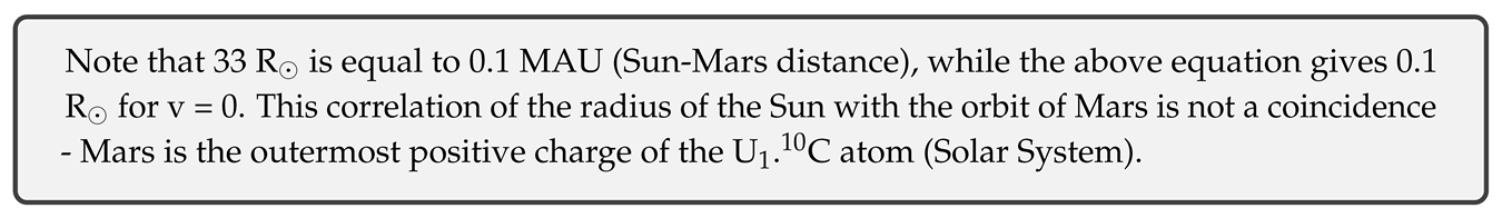
MAU or Mars relative Astronomical Unit is a unit of distance. 1 MAU is equal to the distance of the outermost positive charge from the atom nucleus.
On U scale C atom equivalent, 1 MAU is equal to the distance of Mars from the Sun.
3.4. Weak nuclear decay
Weak nuclear decay transforms a neutron into a proton or vice versa. If these are parts of an atom, this is nuclear transmutation - transformation of one atom of an element into an atom of another element.
With scale invariance of gravitational fields, neutrinos and anti-neutrinos can be, like electrons, bound to atomic nuclei (and, as other fermions, grouped into pairs). In equilibrium, the number of bound electron (e) neutrinos and electron anti-neutrinos within the [primary] radius of the atom correspond to the number of protons and neutrons, respectively. These are, together with nuclei and electrons, primary components of the atom.
Decay process involves annihilation of neutrinos and anti-neutrinos.
3.4.1. decay
Transformation of a neutron to a proton, with emission of excess energy:
Here, bound non-primary e neutrino and bound primary e anti-neutrino annihilate to produce, depending on energy, either an electron/positron (e/e) pair, or up/anti-up quark pair:
In case of electron/positron production, positron further partially annihilates with the down quark (here, both are composite particles), producing neutrino/anti-neutrino pair and up quark:
Neutrino bounds to the atom [as a primary component], while anti-neutrino and electron are ejected in a spin paired state (boson), before separating again:
In case of up/anti-up quark production in the first step, the up quark is absorbed, while anti-up quark pairs with the down quark before ejection:
Outside of atom, the pairing is unstable (short-lived), except at extreme conditions.
Note that, in this case, to conserve equilibrium conditions, one of bound non-primary e neutrinos must reduce its orbit to become a primary component.
decay is the effective transformation of a down quark to up quark of the atom nucleus.
3.4.2. decay
Transformation of a proton to a neutron, with emission of excess energy:
Here, bound primary e neutrino and bound non-primary e anti-neutrino annihilate to produce either an electron/positron (e/e) pair, or down/anti-down quark pair:
In case of electron/positron production, electron further partially annihilates with the up quark (here, both are composite particles), producing neutrino/anti-neutrino pair and a down quark:
The anti-neutrino bounds to the atom [as a primary component], while neutrino and positron are ejected in a spin paired state (boson), before separating again:
In case of down/anti-down quark production in the first step, the down quark is absorbed, while anti-down quark pairs with the up quark before ejection:
Note that, in this case, to conserve equilibrium conditions, one of bound non-primary e anti-neutrinos must reduce its orbit to become a primary component.
decay is the effective transformation of an up quark to down quark of the atom nucleus.
3.4.3. Inverse decay
Transformation of a proton to a neutron by electron anti-neutrino scattering. Generally, this interaction will occur when the atom is not in equilibrium, more specifically - the number of bound e neutrinos is lower than the number of protons.
In this process, e anti-neutrino annihilates with a bound non-primary e neutrino, initiating a decay with electron/positron product:
However, since the number of bound primary e neutrinos was initially lower than the number of protons, now even the created neutrino is bound (as a non-primary component) rather than ejected with a positron:
3.4.4. Electron capture
Transformation of a proton to a neutron by electron capture.
Bound electrons induce the creation of positrons from the atom nucleus, filling its outer energy levels. In low energy conditions this may not be possible and one of the innermost electrons may be captured to fill the vacant level. However, the electron in this level is highly unstable, it is attracted to the outer proton core where it partially annihilates with the up quark, proceeding further as decay:
The anti-neutrino bounds to the atom as a primary component, while neutrino gets ejected. Like in case of inverse decay, there is no W boson creation as no positrons were created:
4. Initial structure hypothesis
In planetary systems, outer (gas) planets are [groups of] electrons, while inner (terrestrial) planets are [groups of] positrons whose gravitational maxima have been extracted from the system nucleus to balance the electrons.
A planet can be in 1e or 2e configuration (state), while the star is a superposition of nuclei partons (quarks). Inner and outer dwarf planets in a planetary system are bound anti-neutrinos and neutrinos, respectively.
Primary components of the Solar System are shown on Figure 4.
The current Solar System seems to be in a C atom configuration, in transition to Be through decay.
Figure 5 a) shows the configuration of a C atom (stable on standard scale, possibly unstable on U), on the left is the configuration of positrons, on the right is the configuration of electrons.
Figure 5 b) shows a possible configuration of a C atom at time of inflation (configuration unstable on standard scale, relatively stable on U scale).
4.1. General deduction of quantum structure
Here is an example how the element and exact isotope species can be determined from the number and types of planets.
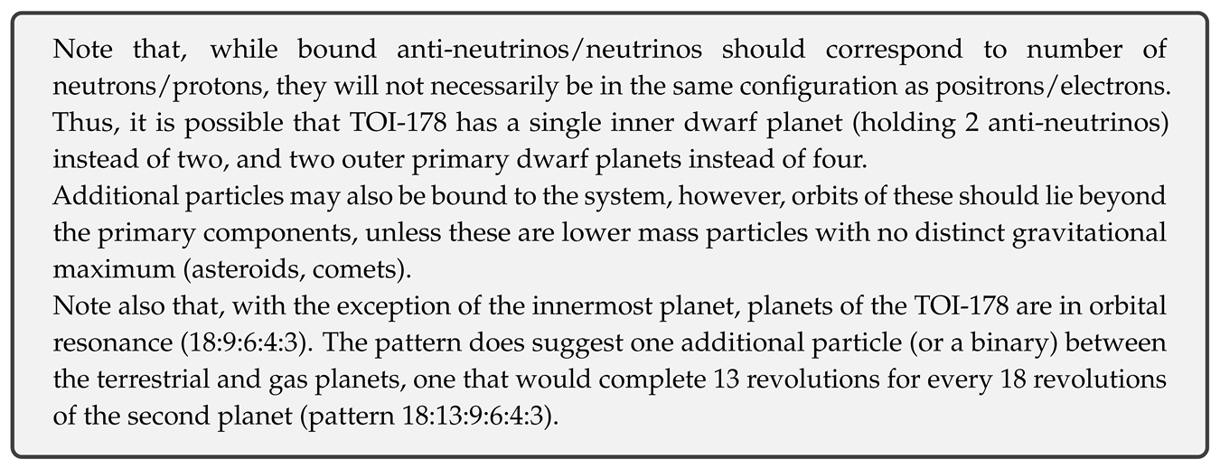
The discovered (star, planets) and hypothesized (dwarf planets) components of TOI-178 system are shown on Figure 6.
With the assumption of maximum 2 electrons (positrons) per planet, the TOI-178 system has these restrictions on the number of particles:
- 2 terrestrial planets limit the number of positrons to 2 - 4,
- 4 gas planets limit the number of electrons to 4 - 8.
Since the intersection of the two groups contains only one solution (4), the TOI-178 system must be a Beryllium atom.
If the number of terrestrial planets corresponds to number of neutrons, this must be a Be isotope.
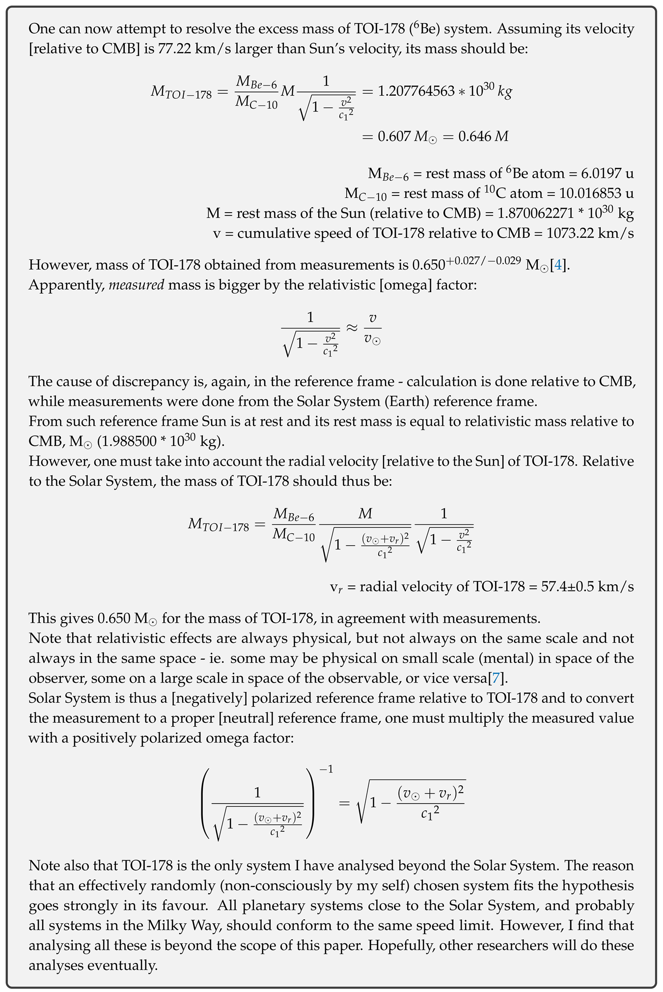
This can be confirmed by comparing the mass of the TOI-178 system [star] with the mass of the Sun. Assuming that the Solar System is C (or Be), the determined mass of TOI-178 (0.647 M[4]) agrees well with the hypothesis.
However, the measured mass is still somewhat larger than expected - reasons for this will be discussed later.
The number of bound [primary] anti-neutrinos should also correspond to number of neutrons, while the number of bound [primary] neutrinos should correspond to the number of protons.
5. Quantum nature
Solar System appears to be a Carbon-10 atom in the current state. Due to extreme conditions some of its components are at the lowest energy level - multiple nucleons have condensed into a single nucleus, orbitals are two dimensional (collapsed from spherical cloud structure), highly aligned (same plane), and momentum carriers are (scaled) point like structures.
Scale invariance of physical laws requires that non-dimensional ratios - those of radii, masses and velocities (energies in general) in two systems of the same species (carbon in this case) but of different scale are equal.
Radius of the outermost electron of C can then be obtained from Neptune spin and orbital radius:
This gives electron radius R = 3.834298096 * 10 m. Note that radii of particles inside the atom can be different than outside of atom.
Generally, radii are affected by kinetic energy and oscillate with mass.
Sun core radius from C nucleus radius and outermost electron radius:
The above gives Sun core radius of 173894.6069 km, or 1/4 of the apparent Sun radius, in agreement with experimentally obtained values of Sun core size. More precisely, this is the Sun outer core [discontinuity] radius and also [approximately] U classical electron radius.

Proton radius approximation:
The factor P/N = 6/4 = 3/2 is the ratio of protons to neutrons in Carbon-10 atom, factor 10 is the number of nucleons (P+N).
The above gives 0.722296 * 10 m = 0.722296 fm for the proton radius, close to experimentally obtained value of 0.8414(19) fm (2018 CODATA[5]).
Same result can be obtained by using spin radii:
A precise value can be obtained by taking into account the influence of quarks instead of P/N (this will be elaborated later):
which gives 0.8426785306 fm, a value in agreement with the CODATA value.
Radius of a proton cannot be absolutely constant, due to hypothesized entanglement between vertical scales, it should probably be shrinking as the Solar System expands during weak evolution of the current state (6p4n).
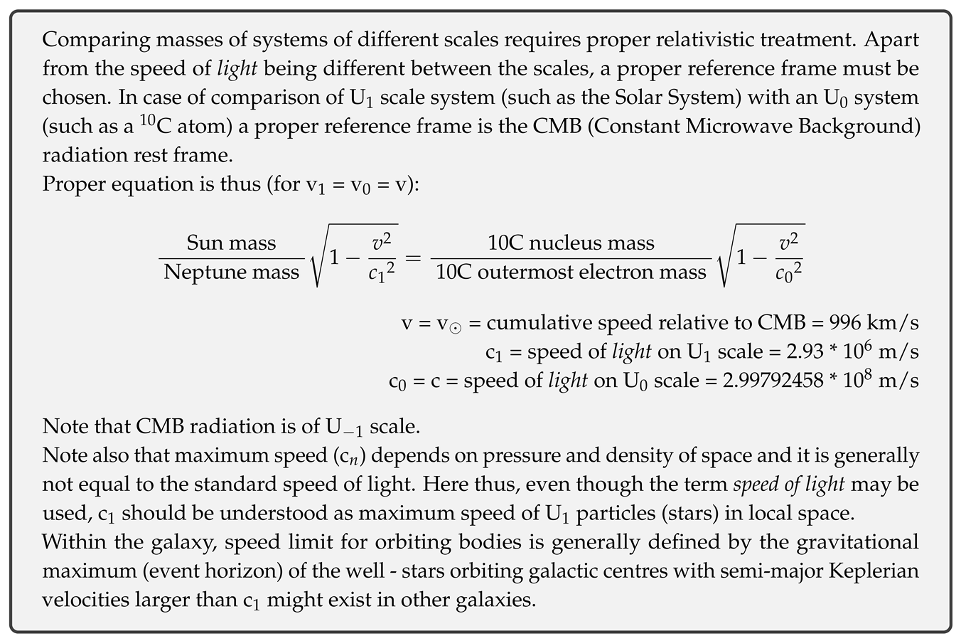
Comparing masses:
This gives:
The above shows mass ratios agree not only to the order of magnitude but are actually very close in value. The excess energy is:
and it must be the locally accumulated relativistic energy of the Solar System (discrepancy arises due to non-invariant reference frames in the mass measurement - the mass of a standard C atom is measured from an external frame, while the mass of the Solar System is derived from within the system and improperly treated as rest mass).
Although the Solar System is at rest relative to us, relativistic energy (deviation from rest velocity) of the system relative to underlying space is always locally real and must be stored somewhere within the system. The likely capacitor is local space (imaginary mass) and apparently the energy is stored in the form of gravitational energy.
From this one can calculate the scaled speed of light for the U scale (c):
If v is interpreted as the cumulative velocity against the CMB (Constant Microwave Background) radiation, a sum of secondary velocity v (velocity of the Solar System against CMB) and primary velocity v (equal to velocity of the local galactic group against CMB), for v = 368 km/s and v = 628 km/s, one obtains:
Obtained c is equal to one of possible values calculated in CR[6], but will also be confirmed here later in a different calculation.
5.1. EH operator validation
If the carbon atom at appropriate density/pressure is the Solar System equivalent, carbon photon is the carbon atom of lower scale (vertical energy level).
One can thus calculate the [average] mass of photons or photon scale particles, ie. electron half-photon:
However, obtained half-photon mass above assumes linear progression of discrete states of scale invariance (vertical symmetry, distance in scale from U to both U and U is equal), which is against the postulates of CR - although this can be the mass of a half-photon in another time (another cycle state).
Thus, CR predicts asymmetric invariance with exponential progression of discrete vertical states. Using this prediction, the masses of standard photon [scale] electron equivalent (half-photon) and carbon graviton have been calculated already in CR (yielding 9.10938356 * 10 kg for the half-photon mass, 1.663337576 * 10 kg for the half-graviton mass), but the values can also be obtained using EH operator.
Using EH factor 6/4 on the orders of magnitude of mass distances:
gives M = 3.910613743 * 10 kg for the mass of graviton in current cycle state, and m = 6.06011796 * 10 kg for the mass of Neptune in current cycle state. Neptune mass is obviously not in agreement with current Neptune mass (unless one considers scaling of the gravitational constant G), however, if this is interpreted as initial real mass component of total mass than it may be correct (see next chapter, where real mass component of Neptune is calculated to be approximately on the order of 10).
Mass of a half-photon can now be obtained from M:
Note that, in current state the ratio of magnitude distances from electron to graviton and from electron to U electron (Neptune) is:
So, for the inverse state (4p6n):
Respecting conditions for the EH inverse, the following values are obtained: mass M = 3.910613743 * 10 kg of [C outermost] electron equivalent in U.4p6n (= M in U.6p4n), M = 9.10938356 * 10 kg for the mass of Neptune equivalent in U.4p6n (= M in U.6p4n), M = 3.719162593 * 10 kg for the mass of graviton in U.4p6n, m = 4.18129939 * 10 kg for the mass of Neptune in U.4p6n (= m in U.6p4n).
5.2. Outermost angular momenta and c confirmation
With the conservation of angular momentum between the Solar System equivalent at U scale (C atom at equivalent density/pressure) and the Solar System, one may attempt to calculate angular velocity of the outermost electron in the C atom:
The above gives the outermost electron velocity in case of conversion of both mass and orbital radius into angular velocity, for a point energy in constant vacuum density.
However, mass M must have been relativistic before the speed limit was reached (vertical energy level changed) and it became the rest mass M.
Thus, in order to get the orbital velocity just before the [vertical] energy level change, rest mass on one scale must be equalized with relativistic mass on another (M = M):
With real mass not participating in inflation (maxima inflate naked), this velocity is the velocity of space, making it potentially valid even in the context of General Relativity (GR).
Using conservation of energy, one can now obtain the velocity of the outermost electron in standard non-excited C atom:
This gives v = 5.585837356 * 10 m/s, for the velocity of the outermost electron of a standard C atom [in Solar System equivalent state].
To confirm validity of the result one can calculate this velocity differently. Introducing the term total velocity (v) as the sum of electron’s spin and angular velocity.
Per CR postulates, every spin momentum must be an orbital momentum. If one assumes that, once captured by the atom, the outermost electron self-orbital (spin) momentum becomes the nucleus-orbital momentum, in ground state (with quantum number l = 0) thus, total momentum of the electron is:
Using m = M≈ M and r = r, this gives v = 8.269308487 * 10 m/s. This momentum in the atom is further divided between orbital and spin momentum. With the ratio of velocities equal to Neptune spin/orbital velocity, one obtains electron orbital velocity:
Two results for the velocity are in good agreement. Small difference can be attributed to uncertainty in vacuum energy density - a value of 9.79 * 10 kg/m would yield the correct value.
From this one can also obtain the scaled speed of light:
The result is in agreement with c previously obtained from relativistic energy of the Solar System (2.93 * 10 m/s).
5.3. The extent of validity of c
The speed c (2.93 * 10 m/s) has been calculated as the relevant quantization constant and speed limit for particles of Sun’s scale in local space. But what is the extent of that space?
Any private space should be associated with a specific gravitational maximum. The Sun should be orbiting this maximum. Therefore, its centre should be the galactic centre, while its radius can be inferred from motion of stars - stars orbiting close to this maximum should orbit at average velocities close to c.
According to measurements, stars with such velocities are concentrated at the galactic centre, near the supermassive black hole Sagittarius A* (Sgr A*). It appears that there are no stars in Milky Way orbiting at velocities ≥ c. In example, as of August 2019, the fastest star orbiting Sgr A* is S62[10].
For the enclosed mass M of 4.15 * 10 M⊙, its Keplerian orbital velocity at determined semi-major (r = 740.067 AU = 1.10714 * 10 m) is:
G = standard gravitational constant = 6.674 * 10 m/kgs
This is a strong evidence for c being the maximum velocity for all stars in Milky Way. The radius of the associated gravitational maximum should thus be the radius of the event horizon for these stars. For mass M of 4.15 * 10 M⊙, this radius (semi-major) is:
5.3.1. Explaining galactic structure
The collapsing spin-alternating gravitational maximum can explain extremes in angular velocities of a galaxy and bright (ignited) regions. It can also explain the young counter-rotating disk(s) of massive stars close to galactic centre[12].
Not only that, it can explain the structure of a galaxy, assuming it is a large scale quantum system:
- the gravitational maximum is oscillating between discrete energy levels,
- there are energy levels it is more likely to occupy than others (explaining discontinuities in density),
- stability of states is different for different galaxies and may differ between levels (stability is inversely proportional to eccentricity of arms),
- an energy level may split into two.
As the maximum is spiralling between states it is affecting momenta of gravitational maxima of smaller scale (ie. those forming stars and planets).
The number of spiral arms is then proportional either to age of the galaxy, or to the number of oscillating gravitational maxima.
Oscillation of this large scale energy should affect [and thus imply oscillation of] smaller scale energy (possibly explaining at least one order of general oscillation of stars, as hypothesized in chapter The cycles).
6. Initial setup and regular disturbances
Solar System is the product of inflation (likely through annihilation) of smaller scale particles or/and deflation [through annihilation] of larger scale particles.
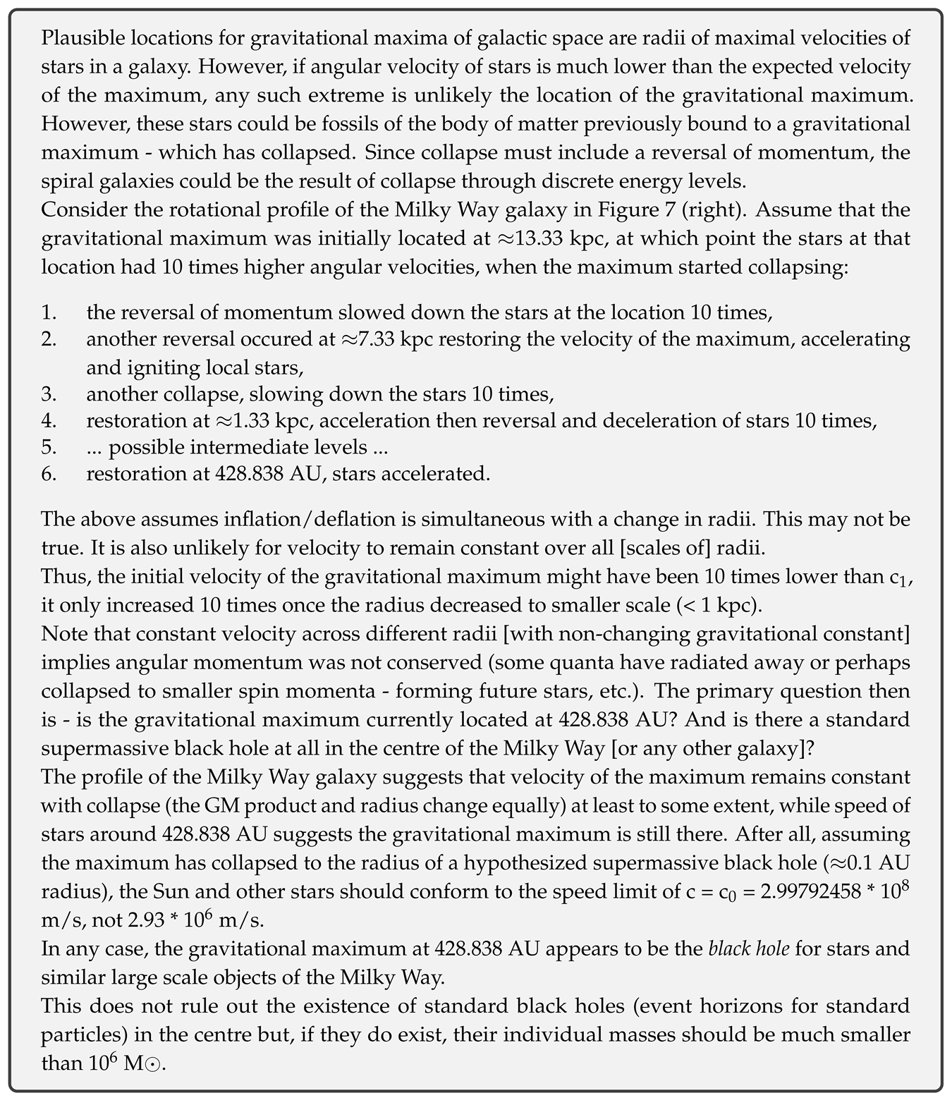
Suppose that at the moment of annihilation the carbon atom was briefly ionized and its mass and charge were condensed into the core when it started inflating. With the electrons inflating along, eventually, the charge would separate from mass again.
The energy provided for transition between adjacent energy levels is generally higher than required, thus, the flattened carbon atom likely expanded to multiple times its current radii, then compressed to current size, trading charge area for neutral gravitational volume.
The atom nucleus in the process expanded up to the main asteroid belt, then compressed, leaving behind orbiting gravitons which collapsed to form terrestrial planets. The collapses were recorded in the Sun, forming discontinuities.
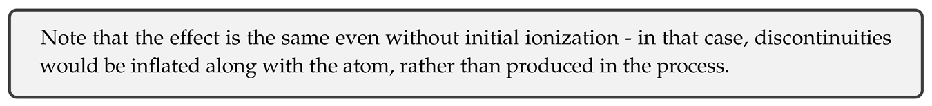
In the transition from charged two-dimensional ring to three-dimensional sphere, equatorial spin momentum has been fragmenting and [due to spin decoupling] spreading to (forming) polar regions.
Latitude variable rotation may have been initially established as the product of conservation of momentum in such redistribution of mass, even if it now may be sustained differently.
Besides the long lived energy level changes, short lived (temporary) inflation/deflation of gravitational maxima will occur with the absorption/emission of [properly scaled] gravitational waves, which may be electrically polarized (electro-magnetic).
Such disturbances will generally occur at regular intervals, with periods generally increasing proportionally to the scale of the system and the scale of disturbance. On the scale of stellar systems, common minimum periods are on the order of millions of years (although smaller periodic disturbances of the system should exist too, these may be of different nature).
Large scale events are always preceded and superseded by smaller scale events so accelerated evolution may proceed for years on smaller scales before the actual disruption on larger scale occurs.
One may now attempt to calculate how much such disturbances last on the large (cataclysmic) scale.
With no change in energy level, orbital areal velocity of bodies, per Kepler’s 2nd law, must remain constant and there should be no change in constitutional mass either.
With a temporary collapse of a gravitational maximum, escape velocity is extremely reduced and orbiting neutral real mass will be increasing orbital radii (although solid mass will generally preserve volume due to smaller scale electro-magnetic and neutral gravitational forces).
In order for this to be a temporary disturbance (no loss of entanglement), collapse must not exceed a specific time period - orbital period of the constituting mass.
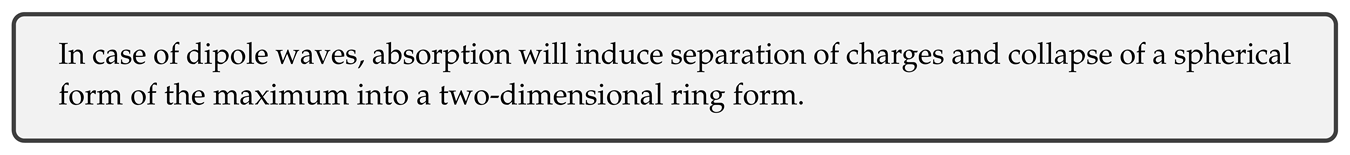
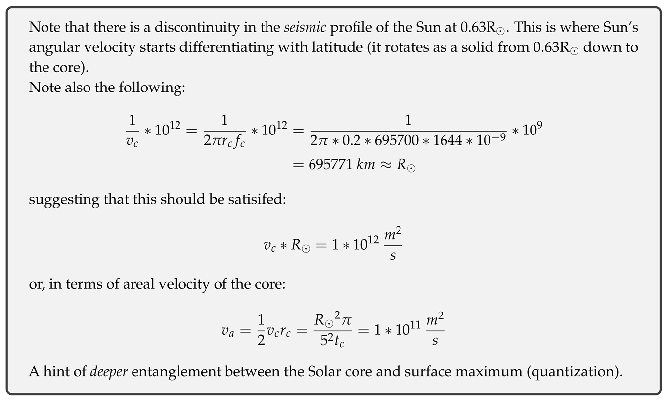
Approximating gravitational maximum as a point maximum (linear ejection of mass from centre) and assuming Sun’s constitutional mass barycentre at the [inner] core radius at the time of collapse of the Sun’s core maximum, maximal allowed ejection distance r at the time the gravitational well is fully restored is:
R = Sun radius = 695700 km
r = inner core radius = 1/5 R = 139140 km
Maximum time between the collapse and full restoration of the well is then:
where f (1644 nHz[13]) is the rotation frequency of the Solar core.
In the context of CR, evolution of systems is not a steady continuous process over all time, but a process with cyclic strong (cataclysmic) changes and a slow (weak) continuous evolution through the cycle.
As I came to realize this I went outside, in despair still burdened by the thought. It was 2 past midnight, I lied on concrete, still entangled with the summer day.. Looking upon the heavens, once again for signs of confirmation I was not expecting to find - "a comet would suffice", I’ve told my self inside. Not a minute away, there it was, a comet passing right in that patch of the sky I’ve been absorbing with the eyes.
Enlightened by the dark, a thought emerged from my self.. Up until recent times my life seemed like a movie scripted by dice thrown by chance, but now, now I did not believe in things anymore, I simply knew..
This life ain’t a fairytale based on true events, but reality based on a fairytale...
7. The cycles
Changes in energy of the Solar System cannot be exempt from general oscillation and remain uniform over its lifetime.
For the Solar System, I hypothesize the following 3 periods (some evidence for which will be provided in this paper, some in follow-up articles) for the first three orders of general oscillation:
- 4.25 * 10 years,
- 25.7 - 25.92 * 10 years,
- 1.512 * 10 years.
These are cycles of existence of the Solar System and its bodies.
Only the 1st order cycle may result in large scale horizontal energy level changes, but all these disturbances are sourced in gravitational stresses and have strong effect on the evolution of the system (and all life within), which is temporarily accelerated at the end of each cycle.
The 1st order period should be interpreted as lifespan of the Solar System as a whole. At time of death, gravitational maxima of the Sun [and likely all planets] collapse exchanging spin momenta for galactic angular momenta. Eventually, this system will couple with real mass and inflate again, probably even into same species (C in this case). It may even couple with the same real mass again, in which case the collapse may be interpreted as temporary loss of consciousness (this recurring coupling should be manifested as reignition of the star after the explosion/expansion of plasma during collapse).
The system of naked gravitons may also inflate or deflate through annihilation or fusion with another system, and then start evolving as new lifeform of another generation or new species, acquiring real mass in vicinity.
In any case, death and new conception are relatively synchronized, and, for these species death is likely not the same as death on our scale. In these species, discarded real mass may be fully reused by another soul - with no temporary and/or spatially large decay and recycling of the mass involved (regarding the individual components of the system, this seems more likely for planets but not as likely for stars as planets are not expected to expand fast with the graviton collapse).
2nd order period should be interpreted as the lifespan of Sun’s core and Jupiter, and possibly all outer planets. Based on current evidence, these collapses should be temporary regardless of nature (death or loss of consciousness). Naturally, even if the large bodies of real mass of gas giants are not disturbed much, the collapses should cause orbital disturbances, and are likely to induce bombardment of terrestrial planets with asteroids.
These should thus be correlated with large extinctions on these planets.
The 1st order period should be interpreted as the lifespan of Earth and possibly all inner (terrestrial) planets (at least in the order of magnitude). Based on evidence, this collapse too is temporary.
Collapse of Earth’s maximum should be synchronized with accelerated evolution of life on its surface. Evidence exists for accelerated human evolution 1.4 - 1.6 Ma[16]. Thus, another such event (effective time compression) should be happening right about now if the 3rd order period is 1.512 My.
All of these periods are time averaged, deviations will exist, but larger periods should be relatively quantized by smaller periods.
Ongoing extinction on Earth may be correlated with the end of a 3rd order period, however, everything suggests this is also the end of a 2nd order period. And, considering the age of Earth and the Solar System, we are likely at the end of a 1st order period too. Thus, major cataclysmic changes should be relatively imminent. While I am convinced that the ongoing 6th major extinction on Earth is sychronized with the end of the current 2nd order cycle, the end of a 1st order cycle may be more synchronized with the end of an additional 2nd order cycle, some 26 million years away.
Currently accepted age of Earth and the Solar System, based on uniform evolution and absolute decay rates of elements, must be wrong. Per CR postulates, decay rates of elements cannot be constant over all time, they must change, either directly with changes in pressure and density of space (ie. at times of graviton collapses), or effectively - ie. with cosmic ray bombardment.
The rates may be relatively constant during weak evolution, however, at the end of a cycle that is synchronized with graviton collapse (ie. the 2nd order cycle) the rates should be significantly, even if temporary, disturbed (accelerating decay). Full collapse is probably not even required. Most likely, the rates are disturbed with the end of a cycle of any order, only the magnitude of disturbance is proportional to the cycle magnitude (period). The magnitude of disturbances will be calculated later.
7.1. Smaller periods
Assuming the ratio of a 3rd to 4th order period is equal to the ratio of a 1st to 2nd order period, and the ratio of a 4th to 5th order period is equal to the ratio of a 2nd to 3rd, the following periods are obtained for the 4th and 5th order:
- 9221.4 years,
- 537.9 years.

While 4th order disturbances could be cataclysmic they (and their effects) should be relatively short-lived and may not generally produce global effects on Earth.
The analysis of recent magnetic excursions and supervolcanic eruptions shows excellent agreement with the proposed 4th order period, as shown in Table 3, for the last 9 cycles.
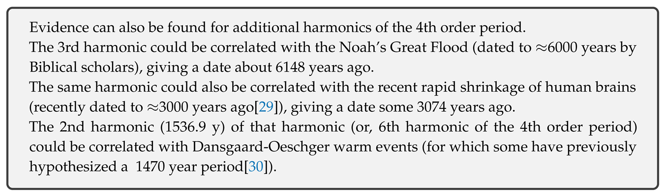
Agreement with hypothesized associated events is remarkable, however, if the proper date for Laschamp is 41.2 ka and assuming Gothenburg magnetic excursion (13.75 - 12.35 ka[26]) is also a part of this cycling, it is possible that the 4th order period of 9221.4 years occasionally (or regularly?) breaks into two equal periods (2nd harmonic) - which could, apart from these two, also explain the 14-12 ka Lake Michigan/Erie excursion, enhanced Be deposition in Antarctic ice ≈60 ka[23] and the Younger Dryas cooling/extinctions ≈12900 years ago[27].

The presence of harmonics probably should not be surprising given how common is resonance in celestial mechanics. Evidence exists for the 2nd harmonic (≈13 million years) of the 2nd order period (25.92 million years) too[28].
Of course, as there are no absolute constants in CR, these periods should be oscillating and evolving, even if weakly. Also, temporary disturbances of oscillation cannot be excluded, as well as the possibility for some harmonics to only be present occasionally (ie. close to events of strong evolution). For these reasons, the hypothesized periods should probably be understood primarily as relatively constant average intervals between associated events at times these are occurring.
However, possible deviation is proportional to period length, and remarkable agreement of the 4th order period with correlated events suggests deviation for the 4th order period may be generally small, up to a couple of decades at most.
Particularly interesting is then the Be enrichment about 9197 years ago[17] (9125 b.p.), which would give year 2046 for the next excursion, assuming there’s no deviation.
8. Effects of mass and gravitational stresses on Keplerian motion
Orbits of bodies in gravitationally bound systems should obey the following equation (orbital law):
G = gravitational constant
where v and r are orbital (Keplerian) velocity and radius, respectively, while M is the mass contained within the radius r.
In planetary systems, most of the mass M is contained within the star, while in galaxies, greatest mass concentration is in the central supermassive black holes (with no outer dark matter taken into account).
However, in both systems, there are orbits at which the equation is apparently not satisfied - v is either higher or lower than expected for detected mass M.
In galaxies, it is assumed that the discrepancy is caused by exotic gravitational mass - dark matter.
In planetary systems, spin of bodies does not obey the equation, but this is largely ignored (not considered as discrepancy), possibly due to current understanding of gravity and accepted theories on formation of planetary systems.
In CR, gravitational force of bodies with a distinct gravitational well may be largely provided by the gravitational maxima so [ordinary] matter content (real mass) may be low.
Thus, a potential equivalent dark matter problem may exist in stars, planets, dwarf planets and larger moons (asteroids and comets are composites of smaller scale wells [held together in most part by electro-magnetic force] so their spin momentum should not be Keplerian, even if their orbit around a body with a distinct maximum should).
The solution for terrestrial bodies lies in the loss of entanglement between space and matter orbitals due to interaction (collision) with other bodies, during formation of the body of matter.
Due to interaction of the atmosphere with a solid body beneath (or its origin), neither the gases of the atmosphere (or trapped particles from outer space interacting with the atmosphere) may obey the orbital law.
This suggests that even below a gas cloud rotating around a distinct maximum at non-Keplerian velocity there should be a solid core, at least in case of a neutral gas, however, angular component of velocity may be converted to radial and then to temperature.
If that gas is in the form of plasma (as in the case of Sun), it is more likely to be entangled with the charge component of a maximum (general force), which then should be the source of its non-Keplerian motion.
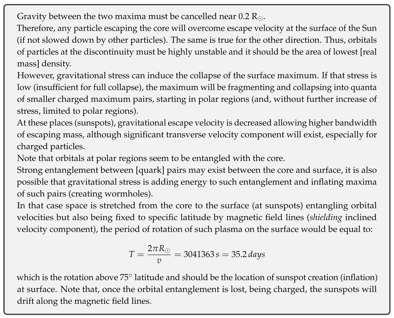
However, stability of a gravitational maximum is proportional to its mass and inversely proportional to gravitational stress.
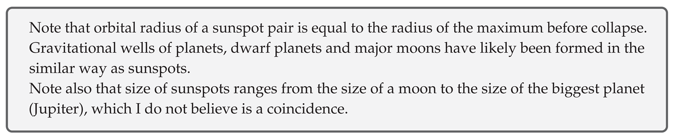
That gravitational stress affects the number of sunspots has already been shown[31], and here I hypothesize that a sunspot pair is the result of a collapse of a quantum of a neutral gravitational surface maximum into a pair of [electrically] oppositely charged and relatively unstable smaller maxima.
A neutral component of a naked gravitational maximum is gravitational energy that may be referred to as dark matter, while visible or ordinary matter is real mass attracted to the gravitational well of such maximum. The velocity curves of the Sun and the Milky Way galaxy likely have the same solution - in the form of gravitational maxima and relativity of their nature due to exchange between polarized and non-polarized potentials of general force.
Rotation frequencies of the Sun (from the core up) and rotational velocities of several spiral galaxies are shown on Figure 7.
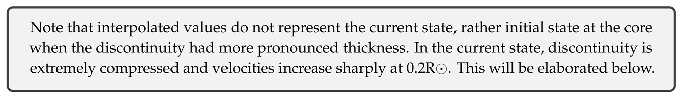
On the left, Figure 8 shows the rotational velocities of the Sun based on rotation frequencies from two independent studies, one for the core (r < 0.2R) and other from the core up (black dots are interpolated values, red dots show velocities at 30 latitude).
On the right, Figure 8 shows the complete velocity curve (with interpolated connection between two curves) and dispersion of velocities (shaded area) due to differential rotation in the convective zone.
What is obvious from the figures is that Sun rotates like a composition of two solid or rigid bodies (diverging only in the polar regions of the convective zone), consistent with condensation of U scale down and up quarks (energy levels) into two ground states (+1s/-1s).
Evidently, velocity curve of the Sun is similar to a typical velocity curve of a spiral galaxy - in both cases there is an initial sharp increase in velocity in the core, followed by a decline, with each next increase in velocity being less steep than the previous one. Note that latitude dependent differential rotation may also be common at specific places in galaxies too.
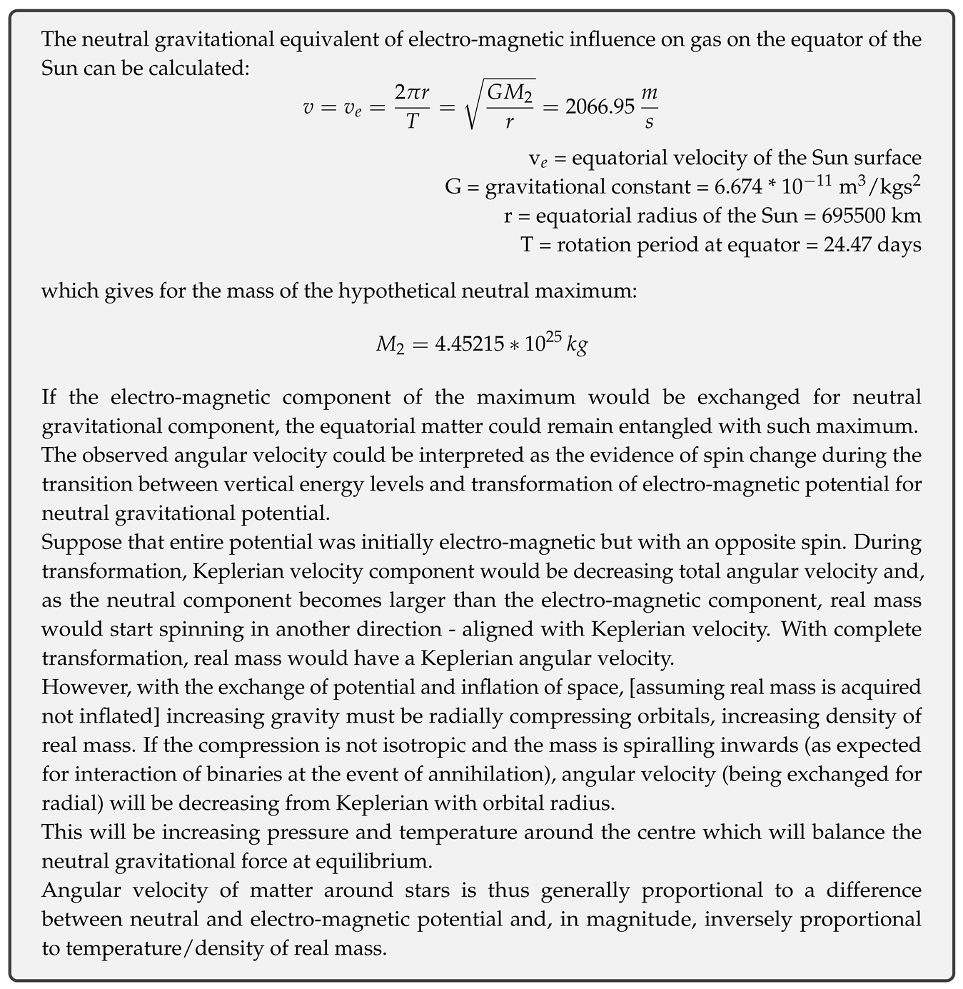
If the spin momentum of the Sun is effectively immune to [large scale] collisions (even if the core would be solid, everything approaching the Sun is vaporized before reaching the surface), the only disturbance of Keplerian orbits must come from incomplete conversion of electro-magnetic potential and increase of temperature.
Assuming that orbital velocity is decreasing (from Keplerian velocity) proportionally to electro-magnetic potential, as hypothesized, orbital velocity of plasma should keep increasing with radius until it becomes equal to Keplerian velocity, beyond which point there should be no accumulation of charge and the radial component of the solar wind should dominate.
Using approximation of the velocity/radius dependence based on the velocity curve of the Sun (up to 130000 km from surface[34]), and equalizing with orbital law:
one obtains the orbit of such discontinuity:
First results from the Parker solar probe indicate a significant rotational velocity of the solar wind around 40 R, peaking at the closest approach. The results indeed indicate a high probability of a maximum velocity around 33 R in case a rigid rotation of the solar wind is maintained up to that point.
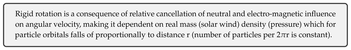
Note that, even without rigid rotation, the discontinuity should occur near the point where velocity becomes Keplerian, otherwise, higher velocity would indicate dark matter presence - another maximum.
If the same is applied to the core of the Sun, the velocity at 0.2 R should be equal to Keplerian velocity. Here, however, this velocity is the sum of Keplerian velocity of the surface maximum and a core maximum. For a surface maximum at R:
s, s∈ {-1, 1}
where M is the mass of the core maximum, s is the spin polarization of gravity of the core maximum and s is the spin polarization of gravity of the surface maximum.
Equalizing this velocity with measured velocity at the core discontinuity:
and setting spin polarization positive for counter-clockwise rotation [of the surface maximum], gives s = -1 and gravitational mass of the core roughly 3/2 the Jupiter mass:
which gives mean core density of:
implying the primary gravitational mass of the Sun is above the core. Difference in mass between the core and outer layers is roughly equal to the mass difference between inner and outer planets.
For the ratios to be equal, core mass must be 3 times higher, which indicates that space has been stretched (compressed, relative to core) from 0.286 R (1.43 * 0.2 R) to 0.2 R. Modifying the equation for Keplerian velocity accordingly would give the initial mass (8.90211033 * 10 kg):
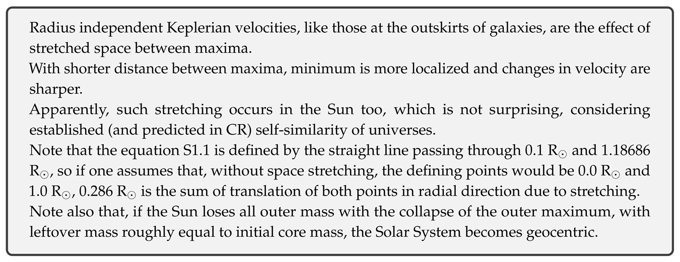
This stretching of space is evident on Figure 9 in the sharp increase of velocity from 0.286 R to 0.2 r. To conserve momentum, this increase in velocities in the inner half had to decrease velocities in the outer half of the Sun, up to 1.18686 R.
Note that slower polar convective rotation could be the result of loss of shielding of the core maximum [charge] due to conversion of potential of the surface maximum (convergence from spherical to ring form).
The specific core discontinuity radius is a result of two competing sources of force, the outer maximum attracting inner maximum outwards while the inner maximum is pulling it inwards (forces cancel near the discontinuity). These are entangled - collapse of the inner maximum would cause expansion of the outer one, while the collapse of the outer one would cause contraction of the inner one.
Somewhere around the discontinuity, conditions may even be suitable for standard life. Note that radius of the core is almost 22 times Earth radius, if density is not isotropic, smaller bodies (moons) might be orbiting inside. Considering momentum of the Solar System barycentre, density should not be isotropic.

9. Symmetry between inner and outer planets
Obviously, inner planets differ from outer planets in terms of energy, size and composition, but the hypothesis of equivalence with (or inflation from) atomic constituents also requires certain symmetry between the two groups of planets - it is predicted that they are oppositely charged and should be spin entangled (or at least were initially).
The orientation of planetary magnetic fields goes in favour of the hypothesis - in one group of planets magnetic north is aligned with mass spin momentum vector, in other it is anti-aligned. Not only that, 3rd inner planet (Venus) relative to the main asteroid belt (event horizon) and 3rd outer planet (Uranus) from the belt seem to have inverted spins relative to other planets in the group. The fact that inversion occurs in the same place within the group (3rd planet relative to the asteroid belt) is further strengthening the hypothesis.
But, as it will be shown later, symmetry, relative to the asteroid belt, exists elsewhere too.
10. Quantization of momentum
Previous works based on Titius-Bode law have shown that planetary orbits are quantized[35]:
More recently it has been shown that distances and orbital periods are consistent with quantized scaling[36] (stable orbits are in harmonic resonances), rather than logarithmic spacing - from the Sun reference frame.

If orbital radii are quantized, orbital (Keplerian) velocities are quantized.
Here, it will be shown that angular momentum is quantized (from a proper reference frame), as well as surface gravity.

Orbital and spin angular momenta are correlated.
Gravitational maxima (event horizons) are, in an ideal case (no electro-magnetic polarization), sphere surfaces with a well defined radius. Mass spin radius and spin velocity of a body (particle) are radius and spin velocity of its gravitational maximum.
Surface gravity of a planet depends on real mass content (defining surface radius) of the well and mass of the maximum. Assuming ratio of used capacity to full capacity for real mass between the planets is roughly the same and assuming ratio of mass of a gravitational maximum to [the square of] its radius is equal between particles on the same energy level, surface gravities of planets will be correlated.
If velocities and radii are quantized, and if momentum is quantized, gravitational mass must be quantized too.
If gravitational mass and radius of a maximum are quantized, its surface gravity must be quantized.
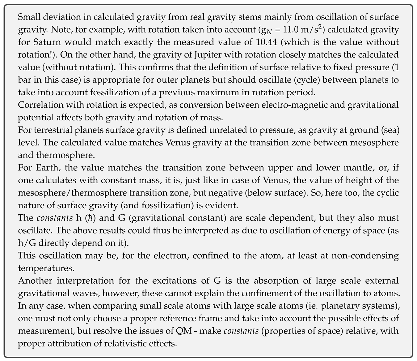
For outer planets, radius of the maximum is here hypothesized to be equal to what is currently defined as the surface radius (1 bar pressure level).
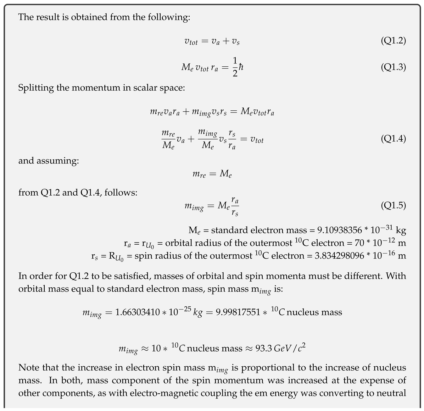
When quantized, orbital angular momentum satisfies the following equation in Bohr interpretation:
where ℏ is a constant, n is a positive integer number and m, v, r are components of orbital angular momentum - mass, velocity and radius, respectively.
Using total mass of the planet for m will not reveal quantization. In example, using Neptune’s mass of 1.02413 * 10 kg and setting n to 5:
one obtains the scaled ℏ (Planck’s) constant for outer planets:
While the result is certainly interesting, the same ℏ will not produce quantized momenta for other planets (it needs to be scaled).
The mass which should produce quantized angular momenta is, as previously established (equation Q1.4), real part of total mass.
However, if surface gravity is correlated with spin momentum, it must be correlated with orbital momentum too, and one may obtain the following equation for surface gravity:
where ℏ is equal to the obtained ℏ above, M and g are Neptune’s mass and surface gravity, respectively. In Table 4, required total mass is the total mass (gravitational energy) required to satisfy the quantization by the QM Bohr interpretation (showing how far it can be from reality) based on obtained ℏ relative to Neptune, calc. gravity is calculated surface gravity, while acc. is the surface acceleration taking rotation into account.
Protons and electrons are parts of two different universes (as difference in scale suggests), so one should use a different ℏ constant for terrestrial planets (proton partons).
The angular momentum of Mercury (m = M = 3.3011 * 10 kg):
gives the scaled ℏ constant for inner planets:
Surface gravity for inner planets, using obtained ℏ, Mercury mass M and gravity g:
In Table 5, showing calculated surface gravity for inner planets, required total mass is the total mass based on ℏ relative to Mercury, while the mirror is an outer planet candidate for [magnetic] spin entanglement.
Quantization can also be shown without using mass (directly), through the volumetric space-time momentum (gravitational momentum):
With h obtained from above, substituting mass with gravity, the equation for gravity becomes:
where g is the gravity of Neptune, or, in case of terrestrial planets, the gravity of Mercury, and it yields the same results.
While the second equation will yield the correct results for gravity, the equation gvr = nh will not, showing the inverse coupling of gravity to momentum:
This gives, for outer planets:
for inner planets:
Now, one can couple mass with gravity:
and obtain relation to Sun’s gravity:
where g is the gravity of Sun at orbital radius r.
For outer planets:
For inner planets:
The above obtained constants are based on total mass, for relative real mass, the quantum of gravitational force () may be treated as invariant between inner and outer planets (with properly defined surface gravity g):
If surface gravity and spin radius are both quantized, then mass of the maximum must be quantized too:
g = gravity of the maximum
M = mass of the maximum
r = radius of the maximum
and, with all three components quantized (m, v, r), the orbital angular momentum would now be quantized if mass would be the same for all inner/outer planets.
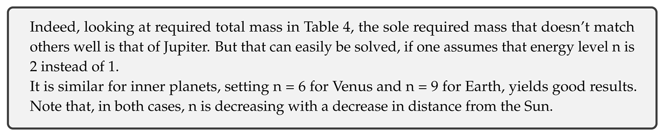
However, masses between planets are not the same. But solution for that exists and it must be in vertical energy (mass) oscillation of particles between generations.
The fact that similar planets (Venus/Earth, Uranus/Neptune) share the energy level (n) fits well with the quantum hypothesis.
The relative high excitation of Mars (n = 10) and no excitation of Jupiter (n = 1) indicates the system is in 6p4n state.
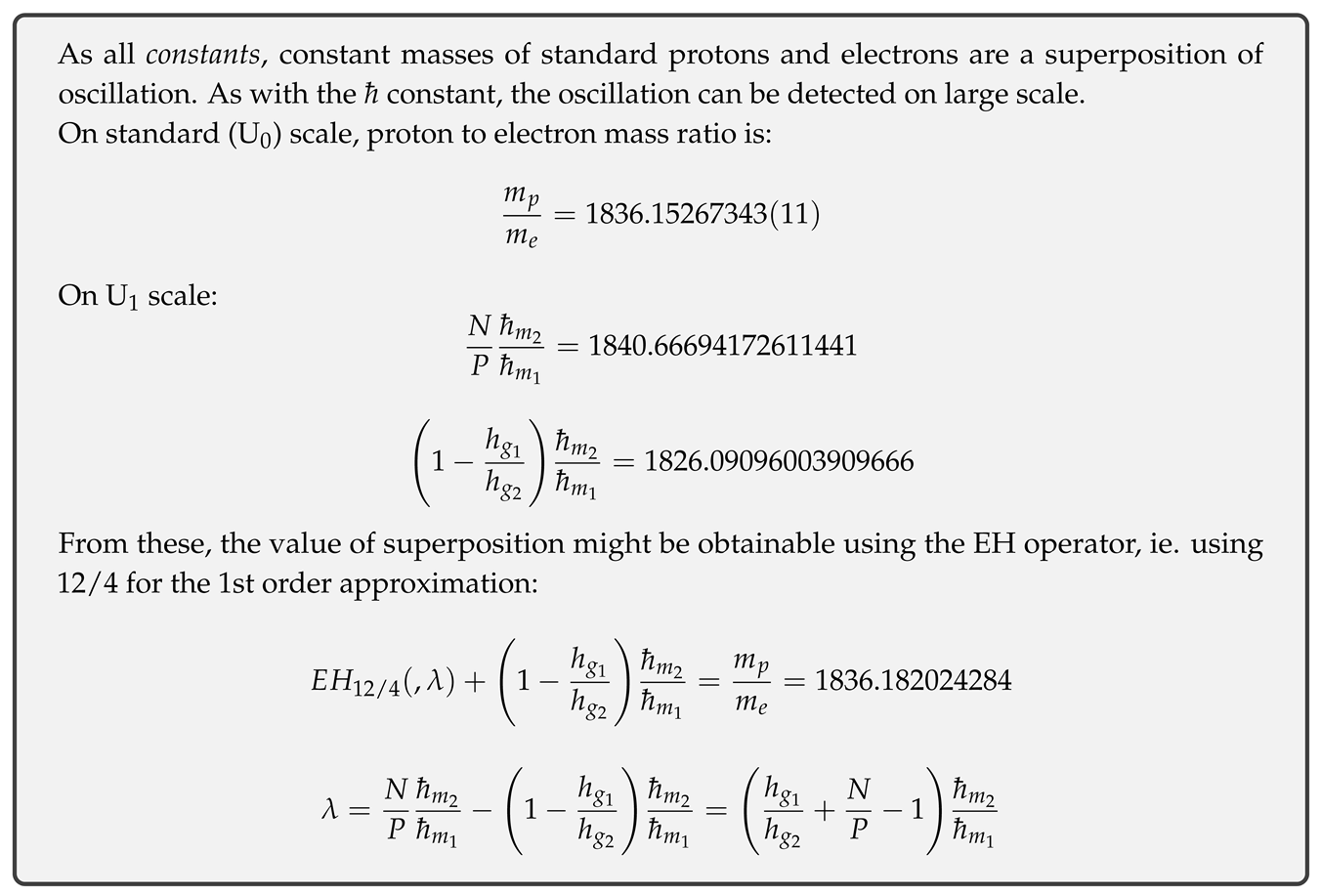
Note that the following should be satisfied (with oscillations in superposition):
where m, m are masses of standard proton and electron, respectively. The factor N/P is the ratio of neutrons to protons in the Solar System.
Some examples of planetary configurations for various states is shown in Table 6.
This shows direct entanglement of standard proton and electron mass with planetary mass and configuration.
The transition from 6p4n to 5p5n state likely includes:
- collapsing (vertical) scale of gravitational maxima,
- loss of one outer gravitational maximum (death of Neptune electron), dead matter remains,
- Mars’ gravitational maximum fusing with one of Earth’s gravitational maxima,
- fusion of Venus’ gravitational maximum with remaining Earth’s gravitational maximum,
- Mercury losing one gravitational maximum,
- small possibility of life changing base to boron,
- formation of a new dwarf planet in the main asteroid belt,
- space between planets expanding (Solar System expanding),
- Solar System increasing orbital momentum (velocity), decreasing spin momentum,
- spin momentum of planets increasing.
The transition from 5p5n to 4p6n state likely includes:
- scale collapse stop,
- loss of one outer gravitational maximum (Uranus e), dead matter remains,
- significant increase of Mars’ gravity,
- death of Mercury, dead matter remains,
- significant increase of Venus’ real mass, decreasing surface gravity,
- no complex surface life on Earth,
- formation of a new dwarf planet in the main asteroid belt,
- further expansion of space between planetary orbits,
- further increase of orbital momentum (velocity), decreasing spin momentum,
- further increase of planetary spins.
10.1. Proper quantization in QM
If one wants to compare the Solar System with a room temperature equivalent of a carbon atom in the context of QM, one must reduce the effects of exchange of em potential with neutral gravitational potential due to condensation and lepton oscillation.
In that case, real mass component of the total initial momentum (Q1.3, Q1.4), which is equal (relatively, but difference is negligible) between bound electrons, is the correct mass to be used in comparison.
Total initial momentum is the angular momentum, it is quantized and for all electrons in ground state should be equal to:
However, generally, total momentum is the sum of orbital and spin components.
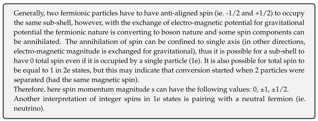
Each quantum sub-shell may contain up to 2 electrons. If these are in condensed (bosonic) form, their momenta are strongly coupled, they will behave as a single body, and the proper equation for the magnitude of total angular momentum per sub-shell is:
R = spin radius
T = spin rotation period
where s is the total [magnetic] spin of electrons in a sub-shell.
Since the value of m here is constant, its value is irrelevant to prove QM equivalent quantization. For the sake of argument, let it be equal to 7 * 10 kg.
Since Jupiter has to be in 2e configuration (even if Solar System would not be the carbon [equivalent] atom), it is appropriate to derive ℏ from its momentum.
Assuming n = 1 (as expected) for Jupiter, l must be equal to 0, with s equal to 1, the ℏ is:
Derived values of l and s (and obtained ℏ using these values) for all the outer planets are shown in Table 7. The obtained value of ℏ for Uranus shows remarkable agreement with Neptune. The ℏ values for Saturn and Jupiter still agree well with Neptune’s ℏ (up to the second decimal), but increase in value with increase in spin radius is obvious. Likely reason for this is oscillation of spin velocity (radius) as noticed previously in quantization of gravitational momentum. Note that this is equivalent to ℏ oscillation, if one is to conserve discrete quantum numbers.
However, the orbital radius oscillates too. Note that orbital velocity is almost equal to spin velocity for planets in 2e configuration (Jupiter and Saturn). Setting orbital velocity equal to equatorial spin velocity and decreasing spin velocity proportionally yields much better results for Jupiter:
v = 12571 m/s
and, similarly, for Saturn:
v = 9871 m/s
One may attempt to do the same with positive charges (terrestrial planets), however, here, determination of spin radius is more challenging and spin rotation period is not primordial.
Instead of using matter velocity, better results should be obtainable using space (Keplerian) velocity at R (which is primordial):
G = G = standard gravitational constant = 6.674 * 10 m/kgs
One possible configuration is shown in Table 8 (with l and s of Earth/Mercury mirroring Saturn/Jupiter, Venus/Mars mirroring Uranus/Neptune, and spin velocity of Mercury set to its perihelion velocity). Note that roughly the same ℏ for Earth can be obtained by setting l to 1, s to -1/2, and spin velocity equal to Keplerian velocity at surface.
However, proper spin radius equivalent to the spin radius of outer planets can be calculated.
From Q1.2 - Q1.5 follows that current mass of a planet is a result of conservation of momentum (and velocity) during collapse of the orbital (non-localized) maximum to a spin maximum:
With m equal to 7 * 10 kg and with the assumption that r is, for all terrestrial planets, equal to current orbital radius, spin radius is:
Here, spin radius should correspond to charge radius. However, obtained radii for Mercury and Mars are much larger then their current surface radii, indicating that either the collapse did not occur at r or there were additional collapses.

Table 9.
Calculated spin radius for inner planets
| n | conf. | planet | total mass M (10 kg) | orbital radius r (10 km) | spin radius r (m) |
| 10 | 1e | Mars | 0.642 | 227.92 | 24851090 |
| 3 | 2e | Earth | 5.972 | 149.6 | 1753428 |
| 3 | 1e | Venus | 4.868 | 108.21 | 1556019 |
| 5 | 2e | Mercury | 0.330 | 57.91 | 12283939 |
However, here the actual value of m is important and another interpretation is possible - the initial assumption of great symmetry may be wrong. While outer planets correspond to electrons of an atom, the inner planets correspond to parts extracted from the nucleus and these may not all be positrons and not even leptons (rather quarks). In that case, chosen m, while it gives good results for Venus and Earth, is not appropriate for Mercury and Mars - it should be smaller.
Assuming m smaller by the ratio of mass between Earth and Mercury, one obtains a charge radius for Mercury of 679 km and 1373 km for Mars, which seem to be appropriate.
10.2. Quantization of radii and gravity
From:
and:
follows:
While, from Q2.1 and Q2.2, orbital radius is:
For outer planets:
Here, square root of k is another quantum momentum magnitude [sum], shown in Table 10. From Q2.3 and Q2.4 follows that surface gravity is quantized:
where g, equal to 43.43 m/s, is the quantum of gravity.
From Q2.3 and with total mass equal to:
follows that spin radius r is quantized too:
Combined with Q2.4 and Q2.5:
For inner planets, the constants are different:
and possible quantization parameters, along with the calculated spin radius, are shown in Table 11. Note that the above parameters for Mars’ orbital radius give a perihelion rather than a semi-major axis, suggesting that it (and generally, planets with large eccentricity) may be in a superposition of two quantum states.
Results for spin radius are obviously wrong, most likely reason for this is the bad h constant as it is based on gravity at surface radius, which, for inner planets, is not defined as the radius of a gravitational maximum.
However, correlation with dipole offsets is still present. Calculated spin radius of Earth/Mercury is almost exactly 10 times the experimentally obtained dipole offset of Mercury (414.7 km).
If the assumption of charge radius being 10 times lower than calculated spin radius for terrestrial planets is valid, somewhat larger current offset for Earth (484.7 km from centre) must be the result of oscillation (superposition) and faster rotation.
Using the radius of a gravitational maximum for Earth (1206115 m), one obtains the proper h constant for charge radius calculation of inner planets:
v = Earth’s orbital velocity = 29780 m/s
r = Earth’s orbital radius = 149.6 * 10 m
g = gravity of the maximum = 274 m/s
n = 3
Results obtained using this constant are shown in Table 12. These are now much closer to dipole offsets. Difference should be attributed to oscillation.
Models of the dipole location of Earth indeed show oscillation, in the last 10000 years it has oscillated from a maximum of 414.7 km (equal to a dipole offset of Mercury) in the western hemisphere to a maximum of 554.7 km in the eastern hemisphere[39].
Dipole offset in current models is thus a superposition (arithmetic mean) of these two maxima (484.7 km).
The agreement of 414.7 km maximum with the dipole offset of Mercury suggests that either:
- the influence of rotation on the offset is negligible,
- rotation stops once the maximum is reached,
- induced currents are created at the expense of primary charge, effectively transferring the charge radius from inner core to outer core.
Possibly, this is the effect of conservation of momentum, where spin of the primary charge is reduced at the expense of core rotation.
10.3. Lepton oscillation model
In the previous chapter it was hypothesized that the discrepancy between the QM model of the atom and the Solar System can be resolved by lepton oscillation.
This can be solely mass oscillation, which requires external energy, or the oscillation of general force flavor which does not require much external energy as mass is inflated with the exchange of polarized (electro-magnetic) potential with a neutral gravitational potential (it does need stimulation though, most likely by resonance - synchronization).
However, while general force flavor has certainly been changed to [dominantly] neutral with a change in vertical energy level, difference in mass between the outer planets is too large compared to a difference in electro-magnetic energy to be explained by general force oscillation alone.
If the Solar System has been inflated, as hypothesized, from a smaller scale atom, then likely there was enough energy for a superposition of electron mass eigenstates.
Taking into account that these electrons are also neutralized, superposition becomes even more likely (charged leptons repel) due to lower energy requirements.
However, the excess energy left after the vertical energy level increase (inflation) might not be the only source of superposition. Most energy in the vertical energy level change is spent on inflation - not flavor oscillation, so even without inflation, the flavor oscillation energy can be provided by the nucleus or absorption of properly scaled gravitational waves.
With no absolute constants allowed and implied oscillation of relative constants, oscillation in the energy of space is predicted by CR.
With no oscillation, in the Solar System, the inner planets would all be in positron equivalent states, while outer planets would be scaled electrons.
10.3.1. The creation
Applying neutralization and lepton oscillation to the model of inflation (vertical energy level change), one can now reconstruct the history of the Solar System development.
With inflation, the [absolute] distance between particles is increasing. Assuming the system started in polarized state, neutralization will be decreasing [relative] distance between equally charged particles.
Based on wave-like appliance of energy, the inflation may have proceeded in this order:
- Nucleus started inflating.
- Jupiter 2e configuration started inflating. Even though 2e composites may have been separated initially, large energy of this configuration enabled the fusion of 2 electrons. With the inflation of Jupiter, 2e positron configuration was inflating. However, this configuration did not have enough energy for fusion and the positrons were left separated enough to form Mars (1e) and Mercury embryo (1e) which may be referred to as Vulcan.
- Saturn 2e configuration started inflating. This one had less energy that Jupiter 2e, but still enough for fusion, while the positrons again, did not - however, the energy was bigger than in the first positron pair, resulting in the creation of Venus (1e) and Gaia (1e, Earth embryo).
- Another 2e configuration started inflating. This one had even less energy than Saturn 2e, and, this time, not enough for fusion, so 2e separated into Uranus (1e) and Neptune (1e). A [relatively] simultaneous 2e inflation resulted in fusion of 1e with Vulcan, creating Mercury, and fusion of the other 1e with Gaia, creating Earth.
Comparing energies of planets, lepton oscillation and the [attempt of] energy balancing is obvious.
Assuming that scaled mass of a standard electron (0.511 MeV/c) is equal to 0.511 * 10 kg, scaled muon (105.658 MeV/c) is 105.658 * 10 kg, while scaled tau particle (1776.86 MeV/c) has a mass of 1776.86 * 10 kg, rough correlation with masses of Mercury/Mars, Neptune/Uranus and Jupiter is obvious.
The tau/muon/electron mass ratios are present within the inner and outer planets:
but also in relation to the Sun:
which suggests that the whole system is in superposition of particles of different generations.
Evolving event horizon (c) model In this model, particles are entangled with different event horizons (still, mostly concentrated between inner and outer charges) impacting their relativistic energies differently.
In Table 13, standard particle candidates are shown for each planet. Rest masses are relative to the possible event horizon of creation, specified in parentheses. Note that original rest mass may be bigger or smaller than relativistic mass, depending on the conditions in the annihilation (creation) event.
Most likely particle candidates are marked green. Rest mass in Table 13 was calculated using proper relativistic factor (Omega factor):
c <> 0
q = sidereal polarization of the reference frame
s = polarization of mass relative to the reference frame
where c = c is the rest velocity of the reference frame (event horizon [fossil]).
Evidently, using most likely particle candidates on the hypothesized particle configuration, the electric charges are in balance, as shown in Table 14.
The configuration gives total 4e charge for inner planets and 4e for outer planets.
The fact that charge configuration agrees well with the hypothesis of 6 particles on each side (Carbon configuration) but the mass for the same particle species agrees well with 4 total particles on each side (Beryllium configuration) indicates that the original hypothesis of C/Be oscillation is correct.
The fact that the sum of charges on each sides is equal to 4, further confirms the hypothesis.
Thus, the Solar System may be interpreted as a hybrid, a superposition of 2 large scale atoms, C and Be.
Is this hybridization unique to the inflation through annihilation of smaller scale atoms, or this is a normal state even in atoms of standard scale?
In CR, of course, the process is scale invariant and cannot be unique to one scale only, even if one cannot set up a proper reference frame to observe it.
The stability of atoms is achieved through neutral energy provided by neutral cores.
It is thus likely that all atoms are oscillating between polarized and non-polarized states.
Note that, with charge extracted, proton core too becomes neutral.
It appears that [outer event horizons of] proton cores favour giving energy to electrons, while neutrons favour positrons (correlated with spin anti-alignment). Asymmetry in neutralization energy between bound positrons and electrons is thus caused in mass difference between protons and neutrons (note that magnetic fields of outer planets are much less subdued than those of inner planets).
With an excess of protons, too much energy on the outer side can cause the ejection of bound positrons and neutrinos, converting protons to neutrons.
With an excess of neutrons, too much energy on the inner side can be enough to fuse bound positrons with the nucleus [core], converting neutrons to protons.
Standard model In this model, planets are simply correlated with appropriate quarks/leptons of the atom.
The correlation is shown in Table 15. If outer particles have to be leptons, possible sums of outer charges are as shown in Table 16. Obviously all masses can be correlated with standard particles (deviation can be attributed to mass oscillation, relativistic energies and possibly non-equilibrium states at the moment of inflation). Mercury and particularly Saturn show somewhat stronger deviation (even if 2e state is assumed, in case of Saturn) suggesting these may be correlated with currently unknown particles (or pairs of unknown particles), however, it could also be a consequence of a non-equilibrium state at time of inflation, ie. a superposition of muon and tau states, in case of Saturn.
But are leptons required?
I have shown in CR, how 2/3 of electron charge can be exchanged for mass, converting electron to a down quark[42] (1/3 e) - where most of the mass goes to a force carrier graviton, giving atomic range for the resulting gravity. If inner anti-down quarks here are a result of exchange of positron charge for mass and this had to be reflected in outer particles, perhaps Saturn and possibly Jupiter represent a pair of muons which have both exchanged charge for mass.
Generalizing the equation (1.4) from CR, the resulting mass after exchange is:
M = mass of the particle after exchange
n = fraction of charge exchanged
q = initial charge
= vacuum electric permittivity = 8.85418782 * 10 F/m
m = initial mass [MeV/c]
G = gravitational constant = 6.674 * 10 m/kgs
C = 1 MeV/c
This, for the exchange of 1/3 charge of a single muon (q = 1 e = 1.60217733 * 10 C, m = 105.658 MeV/c, n = 1/3) gives a 253.3 MeV/c particle. In 2e configuration this would then yield a mass of ≈ 2 x 253.3 = 506.6 MeV/c, very close to Saturn’s 568.34 MeV/c.
Similarly, 2/3 of muon charge exchanged for mass gives 1013 MeV/c, which in 2e configuration becomes ≈ 2026 MeV/c, very close to Jupiter’s 1898 MeV/c.
With these exchanges, total charge on the outer side is:
which, again, suggests that the Solar System is both, a carbon and a beryllium atom at the same time - there are 6 outer particles (as in carbon) but -4 total charge (as in beryllium).
10.3.2. Evaluation of invariance
Correlation between planetary masses and standard particles revealed in the previous chapter is remarkable, not only because ratios of particle masses are equal on both scales, but numeric values seem to be equal between kilograms on one scale and electron volts on another - differing only in the order of magnitude.
This reveals interesting relation between electric charge and speed of light:
where K on the Solar system scale (U) is 1 * 10 Cs/m.
Since planetary masses are derived from GM products, integer value of K must be the consequence of dependence of the gravitational constant G on the speed of light c.
Both values, gravitational constant G and c, have been determined from standard scale (U) experiments, thus:
Mass M of a planet is then determined through gravitational interaction between two bodies, equalizing centripetal force with gravitational force:
where r is the distance [from centre] to the orbiting body [centre], and v is its orbital velocity, and, in case of planets, also the fossil of the rest velocity of the gravitational field line (orbital maximum) before the collapse into a spin (satellite) maximum.
Equalizing centripetal force with electro-magnetic force:
Now equalizing M (gravitational mass) and m (charge mass):
10.4. ℏ constant weakness
Obvious dependency on the order of mass magnitude makes ℏ a weak "constant", but at the same time explains why planetary orbits appear discrete while the orbits of small satellites seem unlimited. Obviously all masses m > 0 must have a quantized momentum.
11. G relativity and equivalence with gravity
If gravity is quantized and total mass M derived from gravity does not reveal quantization of angular momentum, apart from ℏ scale dependence (oscillation), alternative interpretation is a variable gravitational constant G.
It is then a property of a gravitational well (maximum) and it depends on its scale.
Orbital angular momentum (Bohr interpretation):
multiplied with (surface) gravity is:
Fixing g on the right side (ie. M = mass of Neptune, g = gravity of Neptune), multiplying with R/R:
Fixing R in the numerator (ie. R = radius of Neptune) and equalizing with Newton gravity:
Gravitational constant is:
v = orbital velocity
r = orbital radius
R = radius of the planet (spin radius)
Here, v, r and n are variable. One might then consider ℏ a relatively strong constant, but g and R are weak.
It has been shown that g alternates between two values (one taking rotation into account and one without it). The following can be concluded:
- all planets have mutually entangled properties,
- past/future state of g/R is fossilized (memorized) in rotation period,
- gravitational constant G of a gravitational well depends on its own place in a larger gravitational well.
Note that G of a planetary gravitational well is here derived form its orbital momentum in a larger well, rather than its spin momentum.
Planets are orbiting stars, but their bodies are also orbiting their souls (gravitational maxima). Mantle of a planet can be interpreted as a moon to its core, just like a moon can be interpreted as a collapsed gravitational maximum (event horizon) of a planet. In that system, mantle/moon is the planet and a planetary core is the star.
In case the planet is not fully developed (has active moons - in case of inner planets, or doesn’t have active moons - in case of outer planets), mantle layers are [relative equivalents of] asteroid belts and moons are [relative equivalents of] the planets charged oppositely to the outer core of the planet.
Thus, there are gravitational constants relative to that system (note that every spin momentum is orbital momentum - even though the surface and the centre are entangled, propagation of changes is not instant = there are no absolute point particles).
Current value of the standard gravitational constant (6.674 * 10 m/kgs) was commonly measured on Earth’s surface and is relative to an absolute reference frame. In interpretations where G is not scale invariant, proper G for gravitational maxima of inner planets can be obtained from surface gravity and real mass (m):
Assuming speed of matter (real mass) is significantly lower than the Keplerian speed of the maximum (generally valid for matter of solid bodies):
m = real mass of the body relative to [the scale of] its gravitational maximum
r = radius of the gravitational maximum
T = weighted average period of rotation of real mass
R = surface radius
from (G1.1) and (G1.2) follows:
with M calculated, one can now obtain G through (G1.1):
Note that this can also be written as:
substituting middle term for g:
v = matter (real mass) rotation speed at the gravitational maximum r
This relation is now equivalent to the obtained relation for G from orbital momenta.
Note that for Earth, where r = 1206115 m (≈ inner core radius) and T = T = 24h = 86400 s:
which would match exactly the gravity of the inner core [maximum] with mass M equal to previously calculated real mass of Earth (m = 6.95 * 10 kg):
With r and mass remaining constant, increase of g must be the result of increase in gravitational constant G.
The value of the gravitational constant G for Earth’s maximum, with g = 274 m/s (presumed primordial state):
Gravitational constant should not differ much between terrestrial planets. Therefore, solid real mass of these planets should have roughly equal period of rotation (T) to Earth’s rotation period if the ratio of filled capacity to total capacity of the well is equal.
Note that real mass relative to gravitational maximum can also be calculated from equations given in CR:
with:
real mass is:
c = Keplerian angular velocity of the gravitational maximum = 18178.98 m/s
m = M = 5.9723 * 10 kg
From the perspective of a maximum, obtained real mass is the mass of all acquired matter (from our perspective, real mass = M = 5.9723 * 10) kg).
From our perspective, real mass relative to the maximum should probably be interpreted as a quantum of mass that would trigger maximum (graviton) collapse/expansion to another orbital energy level, or ionization of the system. The slower the rotation of real mass of a terrestrial planet compared to Keplerian velocity of the maximum, the less energy is needed for the transition.
The increasing relative retrograde motion of real mass can thus be interpreted as induction of pressure on the graviton.
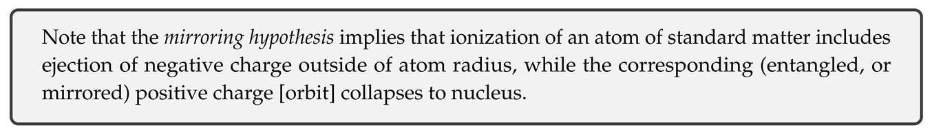
11.1. Correlation with extinctions
As found previously in CR and here, changes in local (spin) energy level of a maximum (or graviton, in general) will fossilize the level as a discontinuity in the celestial body.
For Earth, the required quantum of energy (relativistic mass) for orbital energy level change (ionization) has been calculated in the previous chapter to be equal to 6.95 * 10 kg.
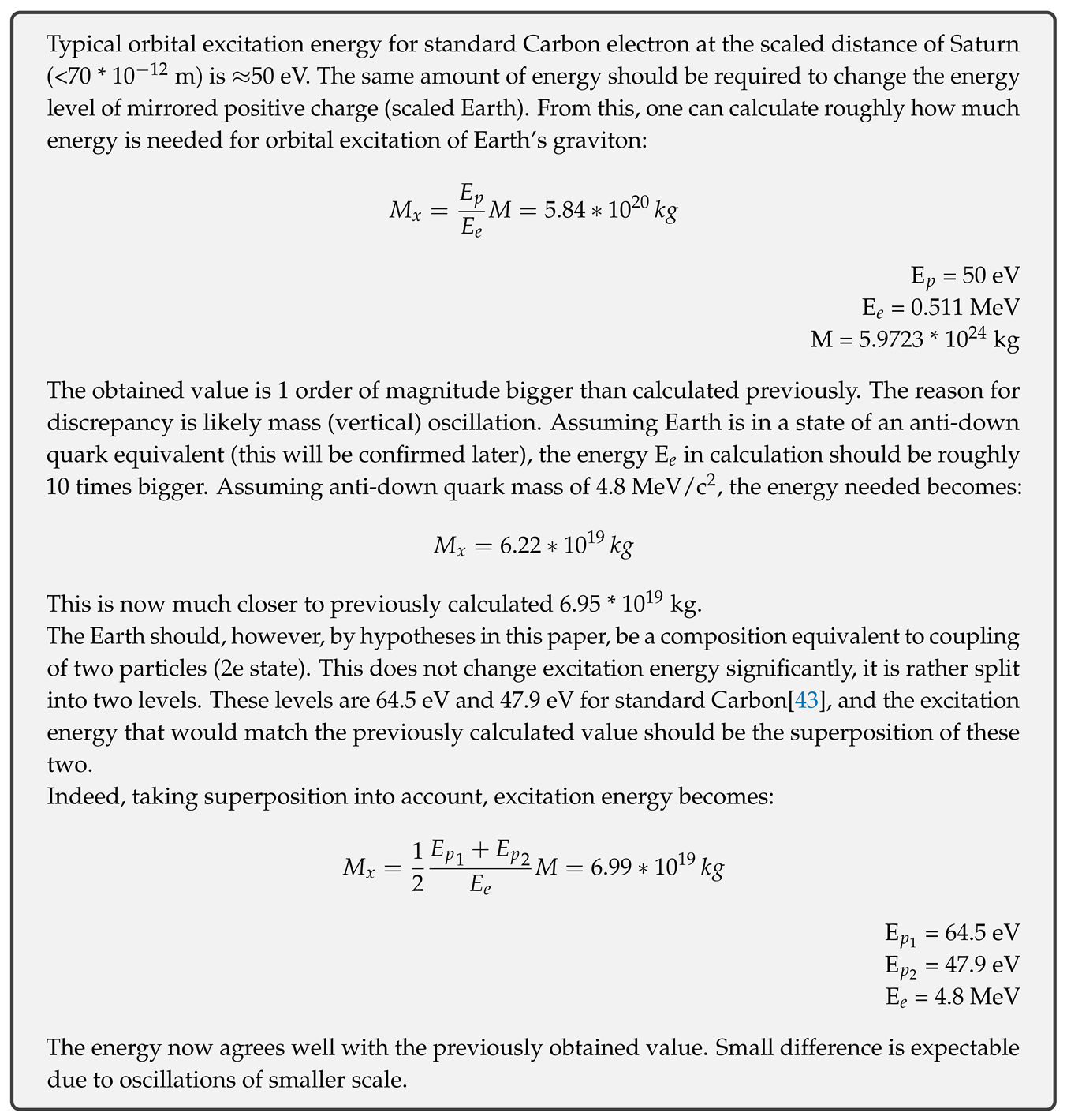
This is a very interesting number considering asteroid impacts are correlated with major massive extinctions.
In example, estimates for the mass of the impactor responsible for the Chicxulub crater range from 1.0 * 10 kg to 4.6 * 10 kg[44].
To trigger a change in orbital energy level, required locally relativistic velocity of such impactor, assuming its rest mass is equal to 4 * 10 kg, is:
m = impactor mass = 4 * 10 kg
m = required relativistic mass = 6.95 * 10 kg
c = Keplerian angular velocity of the maximum = 18178.98 m/s
Interestingly, this is within the range of typical velocities of Earth’s orbit crossing asteroids (12.6 - 40.7 km/s[45]) and comets (16 - 73 km/s[45]). In fact, it seems quite likely that the Chicxulub impactor had the required energy to trigger the change.
However, this approach is flawed - apparently, most asteroids and comets would have enough energy to trigger the change regardless of rest mass. If asteroids and comets have accumulated relativistic energy, it must be the energy relative to Solar System space, not Earth’s space.
Assuming the speed limit is the Keplerian velocity of the Sun’s maximum:
G = 6.674 * 10 mkgs
M = 1.988500 * 10 kg
R = 695735 km
required impact velocity becomes:
This is the average velocity of the solar wind.
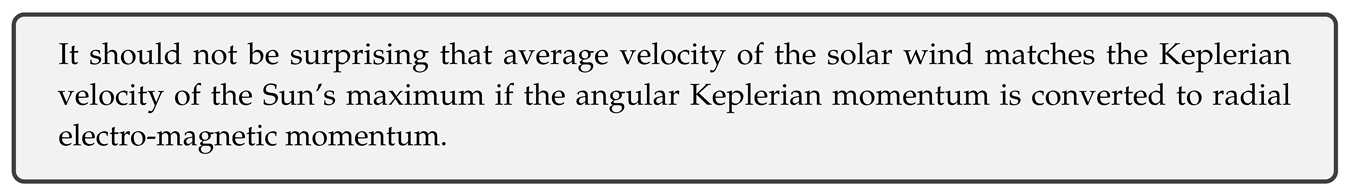
Now this raises a couple of interesting questions:
- is it possible for a coronal mass ejection (CME) to accelerate the asteroid or a comet to required impact velocity?,
- does CME itself represents accumulated relativistic energy in this case (ie. through implantation[46]), at least in part?,
- is a rocky/icy impactor even required - perhaps the CME itself can produce the crater?
- is mass the sole requirement for energy level changes?
The 3rd seems unlikely, especially if there is no temporary collapse of Earth’s magnetic field. However, magnetic field reversals could be coupled with strong CME’s, and research shows that CME’s can produce significant land erosion and ejecta with no protective magnetic field present[47]. Geology can probably rule out this possibility due to a difference in end products between different impacts.
The CME would certainly accelerate an asteroid on its path away from the Sun. If massive impacts are correlated with energy level changes of large scale gravitons, it is possible that it is not solely the amount of energy that matters, but what kind of energy too - electro-magnetic or gravitational?
On standard scale the electro-magnetic energy of photons is the dominant energy triggering energy level changes, on the scale of planets, dominant energy should be gravitational.
However, both energies should be involved as electro-magnetic energy is not absolutely absent, it’s certainly not negligible in case of Earth. On the other hand, one type of energy can be converted to the other at time of impact.
Energy level changes of Earth’s graviton mass radius and charge radius might not be well synchronized relative to standard scale. Thus, collapse of the magnetic field (collapse of charge energy level) could precede the inflation of a graviton mass radius.
Evidence suggests there may have been multiple impactors at different locations at the time of the Cretaceous-Paleogene (K-Pg) boundary formation. A potential impact crater significantly larger than Chicxulub formed at the same time has been identified[48], suggesting significantly bigger impact energy.
However, the Earth is still active (alive) - Earth’s maximum (graviton) is likely still present within Earth. If there was no ionization, were there local (spin) energy level changes?
Assuming energy requirement scales with orbital radii, the required energy for local changes can be calculated:
R = r = Earth’s graviton radius = 1206115 m
r = Earth’s orbital radius = 149.6 * 10 m
M = 6.95 * 10 kg
The Chicxulub impactor apparently had the required energy for such changes.
If similar energies are involved in all major massive extinctions, discontinuities within the Earth should be correlated with major extinctions. This is indeed confirmed in another chapter (Earth as a living organ(ism) > Future development, neurogenesis > Correlation with mantle layers).
There are potential impactors of similar size crossing Earth’s orbit, ie. 1866 Sisyphus.
However, there are multiple energy levels and energy difference between some could be lower than calculated M.
As changes in energy levels are correlated with Earth’s formation and evolution, the energy requirements are probably generally decreasing with time.
Note that energy levels have orders. So far two orders have been calculated, but the 3rd order too could have a significant impact on the planet, assuming equal scaling:
Apparently, we are currently experiencing a major massive extinction on Earth. If these are relatively synchronized with impacts, perhaps one should not be surprised if the 99942 Apophis asteroid (with estimated mass of 4 * 10 kg[49]) is accelerated and deflected toward Earth at its close approach in 2029.
It might not be the CME that is coupled with such impactors, rather a large scale graviton ejected from the Sun. This could make coupling much easier. If the graviton is ejected as a wave and has energy similar to, or compatible with, that of the asteroid, it will likely collapse and couple with the asteroid at the encounter. The graviton will impart momentum on the asteroid, affecting its orbit.
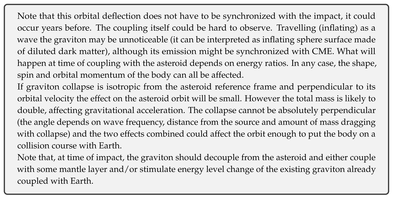
It cannot be excluded that the Moon too has a role in these events. Moon graviton collapse followed by wave-like inflation, asteroid coupling and Earth absorption is an alternative interpretation.
It is possible that one (ie. the Moon) is involved in electro-magnetic energy level changes, other (ie. the Sun) in gravitational.
11.2. Evidence for a constant change of G
The amount of variability in G will depend on the context. Large variability is expected when G is taken relatively to a particular discrete vertical energy level, assuming no change in units.
However, even when G is considered invariant (whether on a particular scale or across different scales) it should not be considered absolutely invariant across all of space and time. In equilibrium conditions it should generally oscillate around some mean value (which itself may change or oscillate over space/time) - the only question is the magnitude of changes, which, however, in equilibrium, may be relatively small within a particular scale.
According to CR, gravity commonly exchanges with electro-magnetic force. Therefore, G should generally increase at the expense of the Coulomb constant, although changes in space/time cannot be instant and some phase shift at distance will exist.
In a bound configuration such as a Solar System, change in G of local space will be reflected in (or synchronized with) changes of orbital momentum.
Taking mass and distance into account, major influence on G on Earth is the interaction with the Sun (multiple orders of magnitude larger than the Moon and planets).
The G constant should thus oscillate, with the 1st order oscillation due to Earth’s elliptical orbit of the Sun.
In the 6p4n (6 protons, 4 neutrons) configuration of the Solar System, the existence of a perihelion and aphelion in the Earth’s orbit should be reflected in two discontinuities of the Sun, at 2/3 R and 1/2 R.
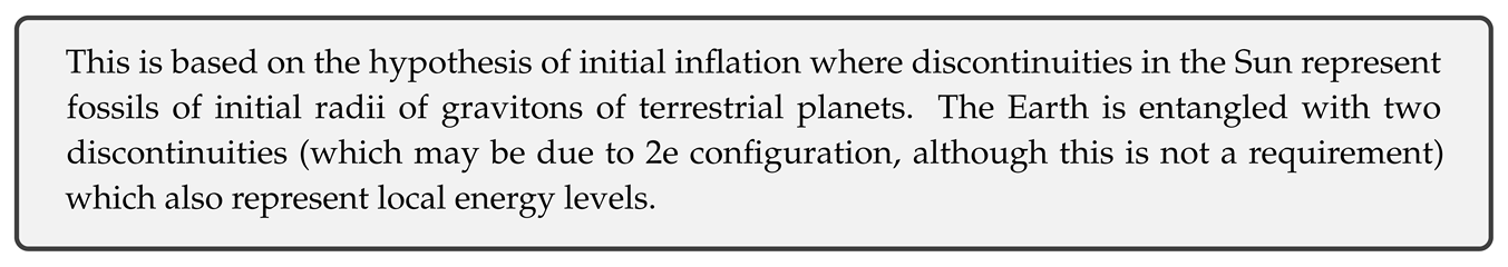
With a change in distance from the Sun, spin velocity of the Earth’s maximum is changing relative to the rest frame of the two discontinuities - its radius is expanding and contracting, directly affecting the local G constant.
Mean change of G due to perihelion is thus:
Change of G due to aphelion:
Giving the total:
v = orbital velocity of Earth at semi-major axis = 29784.485 m/s
v = orbital velocity of Earth at perihelion = 30037.537 m/s
v = orbital velocity of Earth at aphelion = 29538.694 m/s
c = space (Keplerian) angular velocity of the 1/2 R Sun discontinuity = 151.266563 * 10 m/s
c = space (Keplerian) angular velocity of the 2/3 R Sun discontinuity = 230.556106 * 10 m/s

For a mean G of 6.673899 * 10 m/kgs and G = 1.00024, the amplitude of oscillation is 1.60173576 * 10 m/kgs.
Measurements of G on Earth indeed show sinusoidal oscillation, although in previous analysis it has been correlated with the 5.9y (5.899±0.062 y) period oscillation component of Earth’s length of day (LOD)[50].
However, calculated amplitude of yearly oscillation (1.60173576 * 10 m/kgs) agrees very well with the amplitude obtained from measurements (1.619±0.103 * 10 m/kgs).
Figure 10 shows yearly oscillation (blue) superimposed on the 5.9 y oscillation from previous analysis (black). Red crosses are previously measured values of G, plotted with uncertainties (horizontal and vertical).
Yearly oscillation is obviously a better fit, but when linked to orbits of the Earth around the Sun (orbital data taken from NASA Horizons On-Line Ephemeris System[51]) a phase shift of ≈0.6167 y (golden ratio?) is required to match Figure 10 (without the shift the correlation is less convincing with all measurements taken into account).
Interestingly, as shown on Figure 11, with the influence of the Sun removed, leaving only planetary gravitational interactions, best fit requires no phase shift.

11.3. Physical manifestation
CR predicts (implies) oscillation of constants but may generally not offer physical interpretation as these can be diverse. However, relatively physical interpretation must exist. In case of fields the source should be mass oscillation of carrier particles. Here, it would be the mass oscillation of quanta of space (gravitons).
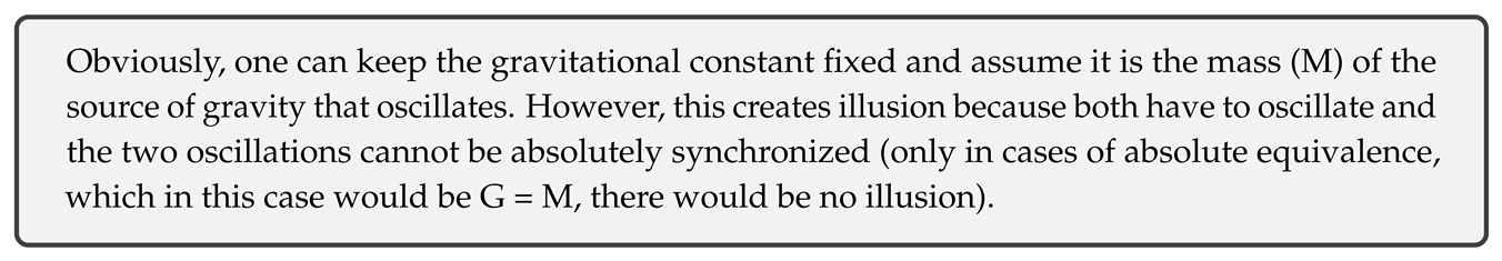
The Earth is most strongly entangled with the Sun (at least gravitationally) but this entanglement oscillates between two energy levels (which can also be interpreted as a relative superposition of the two). This is correlated with changes in Earth’s orbital velocity/distance which are proportional to changes in radius of the Earth’s gravitational maximum (large scale graviton). Oscillation of this radius is proportional to orbital oscillation of constituent quanta of local space resulting in oscillation in density of space at particular distance from the Earth’s centre (which can be interpreted as mass oscillation of constituent gravitons). When this is unaccounted for it will be measured as oscillation of G.
12. Quantization of surface radii
Here are, somewhat empirically determined, equations for quantization of surface radii in the Solar System - may not be applicable to planetary systems in general (with no modification).
Neutral equatorial radius for outer planets:
Neutral equatorial radius for inner planets:
Since both r and M (gravity) are quantized, it follows that R is quantized too by the K constant - other factors (n, p, s, N) are integers.
The above may be understood as the invariant component of the radius during the cycle. Current radius includes a small correction due to oscillation in electric polarization (charge), value of which evolves weakly during the cycle state.
Current equatorial radius for outer planets:
Current equatorial radius for inner planets:
K = 4885811.341 m/kg
K = 2.385039177 * 10 m/kg
M = total mass
r = orbital radius
N = shell number
s = number of particles in a sub-shell
p = state of quantization
n = shell energy level
= angle between spin momenta of a particle pair occupying the shell (in case of a single particle - induced pair by splitting of the maximum)
Calculated radii for the state 6p4n are shown in Table 17, along with measured radii (rightmost column).
Note the quantization of . For inner planets, it is quantized by 90 (any deviation may be due to higher order oscillation).
For outer planets, the quantum is reduced to 1/5 of this value, 18, suggesting, perhaps that the equation for outer planets should be modified, or, instability in radii entanglement, assuming it exists.
Thus, to obtain 90 quantization, one only needs to multiply (quantized by 18) with 5, revealing how it may be entangled with that of the inner planets, as shown in Table 18. Note that s above is interpreted as the number of particles in a sub-shell (Mercury, Earth, Jupiter and Saturn are in 2e states, Venus, Mars, Uranus and Neptune in 1e states).
Interestingly then, the anti-aligned entanglement seems to correspond to entanglement between equal states, while aligned radii entanglement corresponds to entanglement between different states.
12.1. Radius of the Sun and its correlation with proton radius
Original composition of the Sun is probably 6 protons + 4 neutrons. However, 6 positrons worth of charge (inner planets) have been removed to balance the electrons (outer planets).
This makes the Sun neutral:
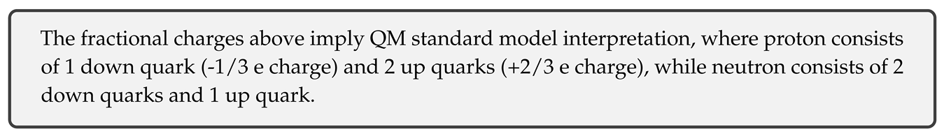
The Sun still consists of both positive and negative charges but their spin effects on radius cancel out. The radius is thus:
where R is the sum radius of negative quarks and R is the sum radius of positive quarks.
As shown in Figure 12, without 6 +e charges, the Sun is a sum neutron consisting of 6 layers, 4 layers containing pairs of negative [down equivalent] quarks and 2 layers (inner and outer core) containing pairs of positive [up equivalent] quarks. Due to condensation, this is the equivalent of a single neutron so 8 negative quarks can be grouped into a single sub-shell as 2 negative quarks, while 4 positive quarks can be grouped into another sub-shell as a single positive quark (8/4 = 2/1).
Thus, the parameter s = 2, while s = 1.
The energy of these two sub-shells must be equal, so M = M = M.
For equal impact on radii, this must be satisfied:
Since M = M = M:
Here p corresponds to number of major (strong) gluons, p to weak gluons, N continues increasing from Mercury (2) so N = 3 and N = 4:
Sun radius then becomes:
Here, ratio r/r is equal to the ratio of orbital radii of the outermost electron (Neptune) and the outermost positron (Mars).
This gives R = 694271.2405 km.
Radius of the sum U scale proton can be obtained by raising the quark factors of R to the power of 2. This is due to the fact that the removal of a negative down quark reduces the negative radius 9 (3) times, while the addition of a positive up quark reduces the positive radius 3/2 times. Distance between charges increases (due to greater difference between them) so total radius is decreased by the sum of these factors.
Radius of a standard proton (U scale) can now be obtained through this equation:
Where r is the Solar System charge radius (Neptune’s orbit), N is the number of nucleons in the Solar System, R is the standard proton radius and r is the standard Carbon-10 (Carbon-12) charge radius.
Using Sun radius R obtained above, this gives:
12.2. validation
Dominant magnetic field in outer planets may be generated by positive charge, in inner planets by negative.
In any case, calculated , as interpreted here, should represent the angle between magnetic dipoles, at least in equilibrium. There are a couple of unknowns though. Is this the primordial angle and is it conserved? In any case, the assumption is that the primordial magnetic field was much stronger and it is then when it could affect planet’s radius significantly.
12.2.1. Mercury
obtained for Mercury (roughly 180) corresponds to ↓↑ spin configuration. This is generally consistent with a low strength magnetic field.
12.2.2. Venus
for Venus (0) suggests a relatively strong magnetic field. Currently, however, except for the induced one by the interaction of the solar wind with Venus’ ionosphere, Venus does not have a strong internally generated magnetic field of its own. The are a couple of explanations for this state:
- it is a result of advanced stage in exchange of electro-magnetic potential for gravitational potential,
- Venus is in a transition between two states (magnetic reversal).
Both may be true. In any case, its magnetic field may be confined inside the planet.
12.2.3. Earth
Earth’s magnetic dipole is not axial, revealing a primal quadrupole configuration, as expected with 2e configuration. Considering the movement of north and south dip poles and attributing it to imminent collapse, in the primal configuration two major (inner and outer) dipoles may have been separated by 90, equal to calculated .
This configuration may have been fossilized in the inner core anisotropy, as shown on Figure 13.
12.2.4. Mars
Obtained shows primal dipole configuration of Mars mirroring the Earth’s. The configuration may be verified once the magnetic field of Mars is restored to full capacity.
12.2.5. Jupiter
(0) is consistent with ↑↑ configuration and may be consistent with observation, as shown on Figure 14, on the left.
Another possibility is a of 109, which is obtained by setting N = 2 for Jupiter (instead of N = 1, see Table 17), shown on Figure 14 on the right.
12.2.6. Saturn
Saturn’s dipole field is aligned with the rotation axis and highly axisymmetric, while quadrupole and higher components are significantly weaker.
This is consistent with ↑↑ configuration suggested by (0).
12.2.7. Uranus
Dipole centre has a significant offset from the centre of the planet. Assuming primal core-dipole entanglement, may be interpreted as the angle between the equator and dipole rotated by such angle that the [shortest] distance from dipole centre to equator (x) is equal to distance from planet surface to the intersection of the rotated axis and axis translated to centre, as shown on Figure 15.
With an 58.6 tilt of the dipole from rotational axis and no inclination, the offset = x = 0.38192 R.
With an inclination of the dipole from rotational axis equal to 1.82, the offset is equal to 0.353 R, in agreement with NASA/GSFC-O model[54].
12.2.8. Neptune
Similar to Uranus, the dipole has a significant offset from the centre. Using the same method as in case of Uranus, one obtains the dipole shown on Figure 16.
With an 46.9 tilt of the dipole from rotational axis, with no inclination, the offset is equal to 0.12193 R.
With an inclination of 63.2716, the offset = y = 0.485 R (x = 0.244967695 R), equal to NASA/GSFC-O model[55] offset.
13. Earth, as a particle
For positive bodies (terrestrial planets), gravity should generally increase with depth, down to the inner gravitational maximum.
For Earth, gravity of this maximum is hypothesized to be equal to the surface maximum of the Sun (274 m/s) when it is localized - not split into multiple quanta of smaller gravity.
In that case, gravity down to the maximum:
where T is the rotation period at radius r. In equilibrium, T at surface for a solid body is:
while real radius of the planet is:
If nT is const.:
For Earth:
Down to the inner core radius r:
G = gravitational constant = 6.674 * 10 m/kgs
M = total gravitational mass of Earth = 5.9723 * 10 kg
ℏ = = 4.613325255 * 10 m/s
Below r (1206115 m) gravity becomes:
At r (event horizon):
At the event horizon gravity is independent of period and radius:
Below r the space-time gradient inverts and gravity is decreasing until it reaches minimum, afterwards possibly increasing again to next maximum, continuing the oscillation.
Table 19.
Gravity of [naked] Earth
| n | discontinuity | radius (m) | gravity (m/s) |
| 1 | crust surface | 6371000 | 9.82 |
| 1 | crust surface perihelion | 6357000 | 9.86 |
| 1 | real surface | 6307105 | 10.02 |
| 1 | outer core | 3282185 | 37 |
| 1 | transition zone (induced charge) | 1705704 | 137 |
| 1 | g. maximum = inner core radius = r | 1206115 | 274 |
| 1 | transition zone | 852852 | 137 |
| 2? | inner inner core | 603058 | 274? |
13.1. Gravity with acquired matter
A gravitational maximum (soul) will effectively curve space around it. In case of shielding interpretation, acquired matter will not affect the overall curvature of that space as long as gravity of the maximum is greater than gravity of acquired matter.
However, clumping or condensation of matter (non-homogeneous system) can produce measurable effects.
In, addition, core maximum may split into multiple maxima (which may even further collapse to form orbiting spin momenta).
Regardless of interpretation (shielding or no shielding), during Earth’s development and evolution, the graviton has likely been oscillating between different energy levels, accumulating mass at different radii from the centre, leaving behind discontinuities.
Distribution of gravity inside Earth is thus likely relatively wavelike, being cancelled at least at some discontinuities (even if currently not globally), albeit with overall increasing density toward the core. This enables Earth’s mantle to have layers where pressures and temperatures are suitable for complex ecosystems.
14. Earth, as a living organ(ism)
Earth is definitely showing signs of a self-regulated living organism on surface, at least between major extinctions. But even disruptions of that self-regulation can be explained either as a regular component of embryonic development process or as a presence of a disease. These interpretations are not mutually exclusive - both can be simultaneously valid, at least in some cases.
While it may be hard to identify the equivalent of genetic coding in such a large scale organism, it shouldn’t be discarded as a possibility due to lack of imagination, especially when there’s sound logic behind its existence and evidence in its favour.
In all living beings known to man, life is not limited to outer skin surface - in fact, life there is generally least diverse and complex. Higher diversity and complexity on skin surface is generally limited to short periods during embryonic development. The fact that no complex life has been detected on a surface of any planet but Earth goes in favour of this hypothesis.
Existing models of Earth’s interior are mainly based on assumptions on planetary formation that do not involve soul/body coupling and which are certainly not backed by abundant and solid evidence. They are also based on data from seismic profiling which has limited resolution and is prone to interpretation bias[59].
Bias exists in definition of life itself in modern science - apparently there is no solid consensus on required constitution of a living being. But even if there would be one, in current climate, it would hardly allow for Earth to be alive.
However, assuming extroversion and introversion of life can go to extremes, then everything would have to be alive, only differing in the ratio of mental to physical interaction (or amount of life in these domains or dimensions of reality).
With CR, relativity of life is implied - amount of life should depend on a reference frame, so Earth too should be alive.
The entire Solar System is then also an individual organism, and, relative to that system, Sun and planets may be interpreted as organs (physically relatively passive, or extremely introverted, symbiotic organisms).
Obeying the principle of self-similarity, each living organ has an active core, replicating the role of the Sun in the Solar System to localized space-time.
These are, obviously, all extremely introverted organisms. For that reason, creatures of extroverted nature accustomed to absolutism may not recognize them as living beings, however, lack of complexity in physical momenta is simply replaced with complexity in mental momenta - which is reflected in momenta of smaller scale life-forms (or quanta of consciousness) residing inside their bodies. One of these life-forms are humans, who are, relative to Earth, likely its [precursor] neural proteins.
Deeper understanding of organisms of planetary scale (or larger) requires understanding of [discrete] scale-invariance of physical laws. One cannot expect that time for these beings (or communication between their constituent parts - ie. neuron equivalents) flows at the same rate as for organisms of smaller scale (ie. humans), nor that their tissue should look like our tissue (discrete states of invariance imply a difference).
14.1. Rough internal structure
With no apparent complex, stochastic or conscious large scale extroverted physical interactions (apart from electro-magnetic absorption and emission which may be interpreted as communication) present in planets, planets must be extremely introverted life-forms. In such organisms there’s simply no need for limbs and large scale complexity in organismal structure, it is the smaller constituent quanta of these structures that can be complex. And the behaviour of most will be complex (or relatively stochastic) if these are correlated with high introverted intelligence or consciousness of the being.
Most expressed organ of an organism such as Earth then must be the brain, likely organized into layers with possibly minimally expressed gyrification (although that may depend on the stage of development).
Even so, it has to have other organs [or organ equivalents] necessary for the function of that brain.
Most likely blood arteries are underground tubes, with blood being the flowing magma and water (nutrients).

Its blood veins are underground tubes filled with oil (compressed dead carbon matter).
Complex life and networks of interconnected diversity are not limited to surface (epidermis). In fact, surface is likely just a breeding ground for cultivation of precursor neuron cells and proteins of a planet. Most complex life is thus resident within mantle layers where it is protected and not so vulnerable to external influence.
The core of a planet has the role of a heart and geyser eruptions may provide one way to probe the heart rate when the surface is active.

14.2. Age, lifespan and the 3rd order period
The lifetime of Earth is quantized and can be calculated through its frequency of existence.
For n = 2840, and determined T of the 3rd order general oscillation of the Solar System equal to 1.512 * 10 years:
But this should not be interpreted as lifespan of Earth, rather lifespan of the Solar System. I hypothesize that the Earth’s lifespan is equal to T (3rd order period of the Solar System oscillation).
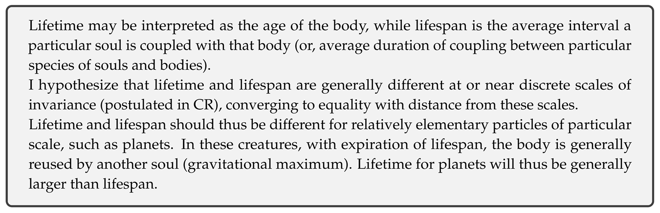
There are at least 3 ways to calculate the 3rd order period of existence cycle T [and thus, Earth’s lifespan], all giving the same result:
14.2.1. Decay rate of Be
Current Solar System state may be C or a superposition of C and Be. In any case, entanglement exists between the Solar System and standard Be. I propose that half-life of Be is equal to the 3rd order period of the Solar System oscillation (in one interpretation, the half-life has been fossilized as the 3rd order period).
Several measurements of Be half-life have been performed.
In example, in 1987. it was measured to be 1.51±0.06 * 10 years[60].
In 2009. it was measured to be 1.388±0.018 * 10 years[61].
Even though half-life of U elements should be consistent during the existence cycle of U, it likely changes during the transition between cycles - T should be understood as the mean value.
For that reason, I do not consider the value from 2009. as the average value through the lifetime of the Solar System. It will be shown later that this value is 1.512 * 10 years.
14.2.2. Heart rate
The average heart rate of Earth can be calculated from the global average period between geyser eruptions:
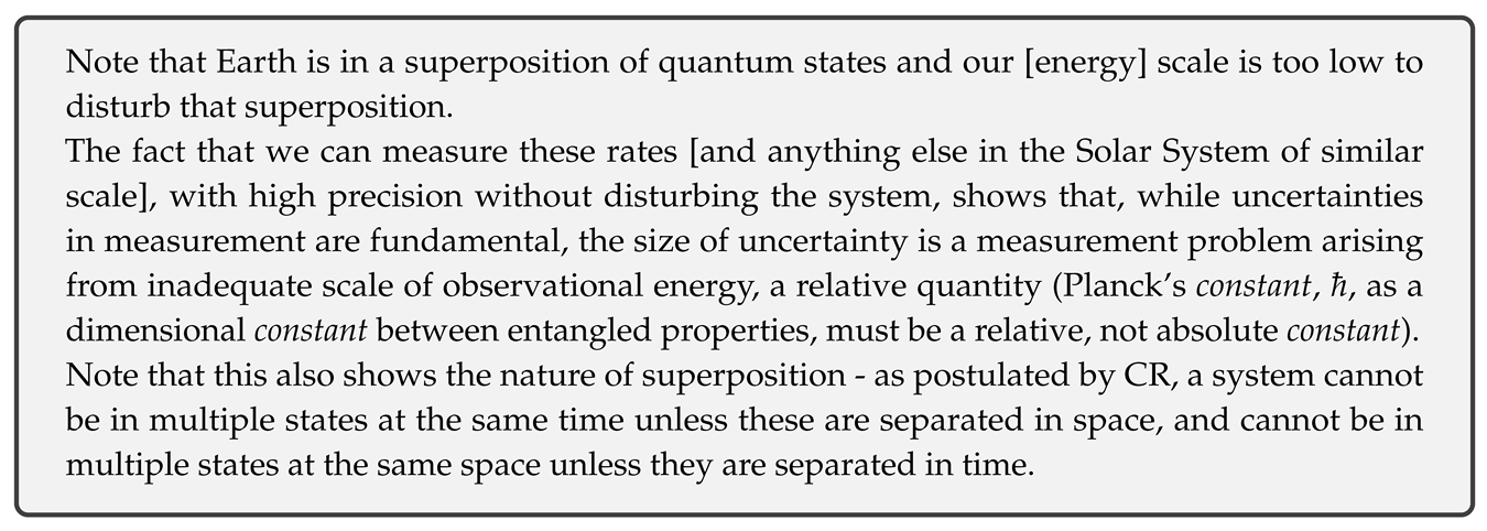
For Earth heart rate = my rest heart rate (76 bpm) scaled:
Given the number of heartbeats EH(1 * 10, 4 * 10) = 2 * 10 and scale invariance of heartbeats, the period is:
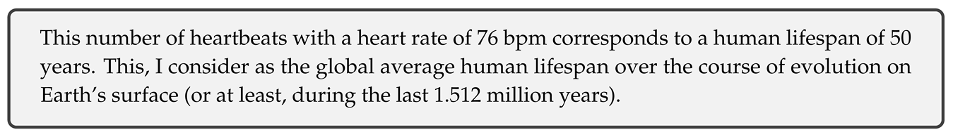
With such number of heart beats[62] (between incarnations), the Earth would belong to, not only mammalian species, but relative homo species.
The 3rd order cycle of the Solar System (1.512 * 10 years) can thus be interpreted as evidence of inter-scales evolutionary entanglement - a man is in its path of evolution between the standard scale carbon atom and the Solar System (relative large scale carbon atom equivalent).
To species accustomed to the concept of birth and extroverted nature it might appear that Earth never fully develops.
This is most certainly not the case - life past the embryonic form for us always results in a change of environment, but this is only due to inadequacy of the uterus to ensure the continuity of progressive evolution, one which includes growth of the physical form.
Once extroverted intelligence evolves into, relatively more energy efficient, introverted intelligence, there is no need for physical growth or reason for most of conventional physical organs.
14.2.3. Speed of time
Space-time may be represented by two dimensions, one positively polarized (space), one negative (time), relative to a neutral one (event horizon in between).
These 3 dimensions are spatially separated and quantized, but they are entangled and may orbit the same body, such that orbital velocity of the event horizon is:
where v and v are orbital velocities of space and time dimensions, respectively. 3rd order space for Earth is 1-dimensional - the Earth is an inflated quantum of space/time orbiting the Sun. Dimensions of [3rd order] space and time of Earth have been further separated during inflation, but they remain entangled. Assuming that space dimension is [at] Earth’s orbital radius, the time dimension should be somewhere in the higher orbit.
Time dimension velocity is quantized by v:
The values in square brackets, depending on the sign, give maximum and minimum values of v during the cycle state. The average (mean) v:
For inner planets, in state 6p4n:
Solar System may also be observed as a hydrogen-like atom, where space, time and event horizon dimensions have been split into 4 component vectors (levels).
The event horizon velocity (derived from v and v), given the orbital energy level vectors for inner (n), outer (n) planets and the oscillatory vector k:
where ⊕ is the sign operator:
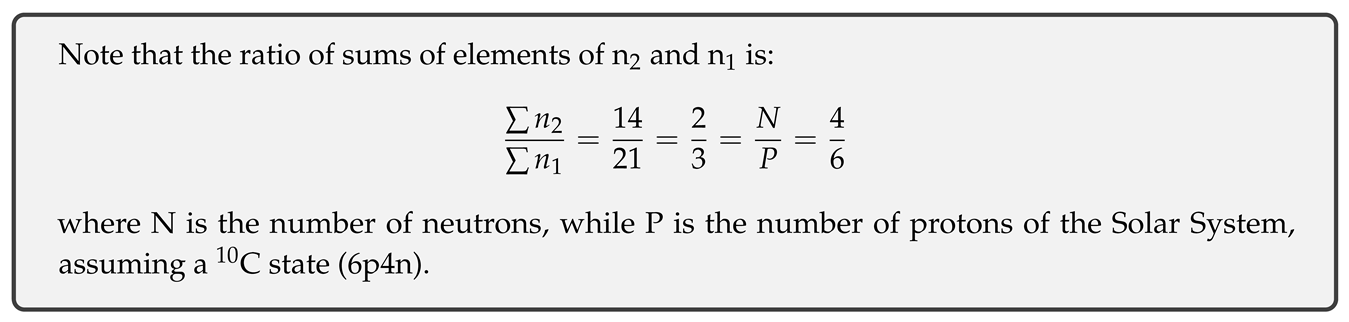
The event horizon velocity (from v only):
where is the Kronecker delta function. Table 20 shows space velocities for inner planets and calculated velocities of time and event horizon dimensions along with their correlation with bodies of the Solar System.
Evidently, the speed of time dimension decreases as the speed of space increases and orbits are quantized and entangled (as predicted by CR):
Orbital velocity of Earth’s space is 29.78 km/s. Average velocity of the event horizon for Earth is 2/3 of this velocity, while the average velocity of time dimension is 1/3 of this velocity:
Orbital radius of the time dimension is the space dimension of Saturn - Earth’s time dimension is entangled with the space dimension of Saturn (time dimension of Saturn is entangled with Earth space dimension).
Average event horizon is entangled with the current orbit of Vesta, the dwarf planet.
Deviation of v from current Saturn orbit is equal to deviation of v from current Vesta:
Speed of time for human bodies (c) is equal to standard speed of light c, given the average life expectancy of 50 years (2*10 heartbeats with 76 bpm heart rate), the 3rd order period of Earth’s existence cycle is:
14.3. Body mass
If Earth is a living organism, predicting real mass of Earth in the same way as it is done with other organisms should give the result of the same order of magnitude (it likely won’t be of equal value as Earth is evolving, gaining and losing mass in the process).
Assuming that Earth is a relative mammal, given the 3rd order existence half-life (period) T of 1.512 * 10 years, mass can be calculated from empirical relationship between mass and lifespan of mammalian species.
Given human adult mass m of 84 kg and lifespan T of 50 years, mass of earth m is:
Not equal to total mass of Earth, but a very interesting result. It is equal to previously calculated Earth mass using non-invariant G, and also a quantum of energy required for orbital excitation of Earth’s graviton.
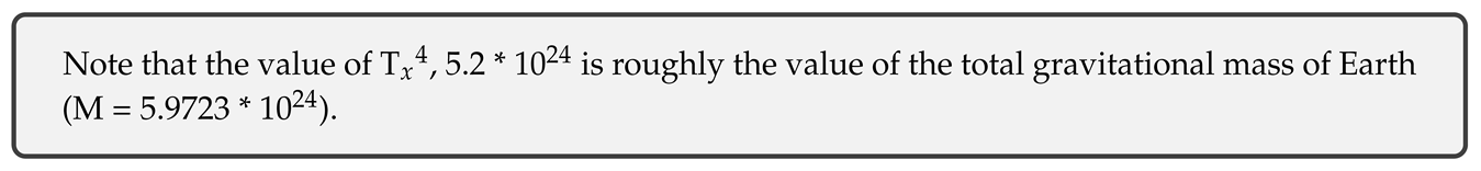
The same mass is obtained using the CR equation for real mass:
where
Using T = 23.9*60*60 = 86040 s, G = G = 6.673899 * 10 m/kgs, r = 1206115 m, m≈ M = 5.9723 * 10 kg:
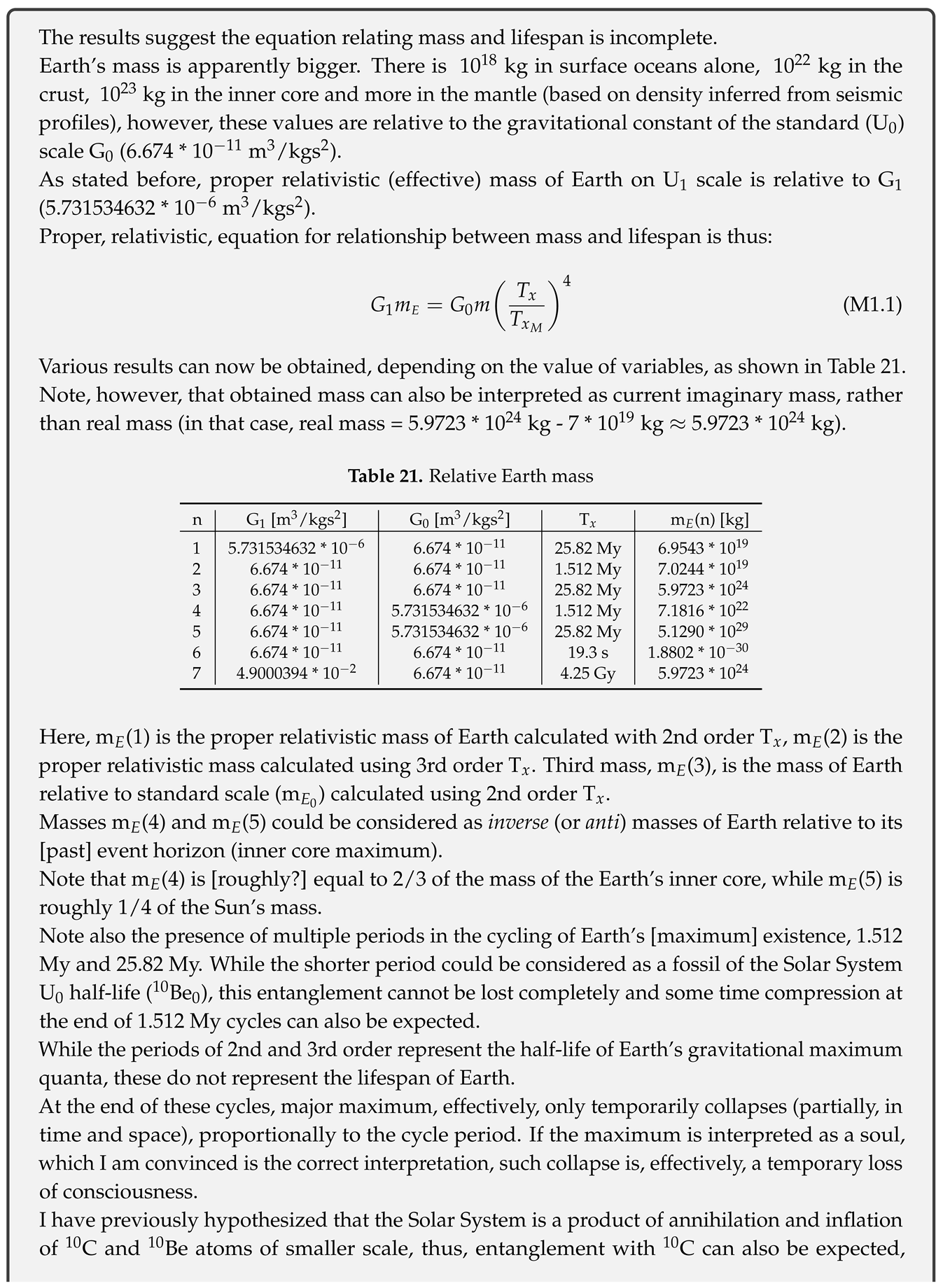
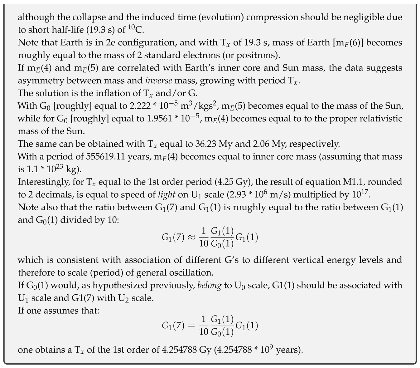
14.4. Future development, neurogenesis
Here I hypothesize that cultivation of life on the surface of a planet is a cultivation of precursor neuron cells and proteins (relative to the planet) which are, at the point of differentiation transferred to planet’s [brain] mantle layers. Similar to accelerated (time compressed) evolution during human embryo-genesis, I hypothesize that effective time compression occurs during planetary evolution too - with the end of each cycle of general oscillation of the Solar System (Earth) and with amount of compression being inversely proportional to cycle order.
The points of differentiation and migration in neurogenesis are major mass extinction events (although limited transfer might occur in smaller extinctions too), which are thus only relative extinctions - life is not completely extinct, it undergoes rapid evolution and migrates away to mantle where it continues evolution.
I hypothesize that Earth’s brain has, like human brain, 6 major layers, and that complete formation of these layers requires 6 major mass extinctions during Phanerozoic.
At this point, there is no doubt that we are amidst an major extinction event, a 6th one.
Being part of neurogenesis, extinction events must be programmed at some level and, at least roughly, periodic.
Extinction events have relative triggers. While in the past these may have been impactors and volcanism, current extinction seems to have an anthropogenic trigger.
Thus, one might conclude that current extinction is not part of neurogenesis, rather a part of unlimited cancer growth. However, tumors in humans are known to induce neurogenesis (it is one mechanism enabling migration - metastasis).
I find the induction questionable though - humans are not consciously triggering neurogenesis on Earth, it is thus more plausible for neurogenesis to be a reaction of the immune system to inhibit cancer growth. Extinctions coupled with neurogenesis go in favour of such hypothesis. In case of cancer in humans though, and at least during adult neurogenesis in humans, the immune system seems to fail to cure or exterminate the cancerous cells in most cases (in case of humans who are cancerous themselves for Earth, I believe).
The immune system of Earth though, should be more advanced, and I believe cancerous homo.beta[63] will be subdued.
Judging by past major extinctions, and correlating with human neurogenesis, these events should be expected with the advancement of planetary neurogenesis:
- increasing rate of volcanism and earthquakes (due to gyrification/formation of brain tissue, incl. fragmentation/cracking of the crust and flooding of the surface, curing cancer?),
- asteroid/cometary impacts (providing energy, acting as specific event triggers - ie. graviton energy level changes, tissue formation with volcanism, curing cancer?),
- water level changes (melting of polar ice to enable migration, flooding of surface with interior water, curing cancer?),
- ocean pH reaching minimum (possibly triggering migration, curing cancer?).
Migration of cells and proteins from surface to mantle layers requires tunnels connecting these regions. Most likely, these tunnels exist on specific places and are recreated or reopened at time of migration. A likely place for such tunnel opening on surface is the south pole, but may exist on north pole of a planet too.
Cells and proteins are transferred with the flow of cerebrospinal fluid (CSF) - a salty ocean. In humans, CSF has a pH of 7.33, and, since pH is scale invariant the pH of Earth’s CSF should be roughly equal. The current acidification of Earth’s oceans will, therefore, probably continue until pH drops to this value, when migration should follow. Afterwards, new surface water may be delivered by asteroid impacts, but it is also possible that some or most of it returns from the mantle.
Based on correlation with atmospheric CO, climate models predict the hypothesized pH minimum in year 2300 AD for an atmospheric concentration of CO of 1900 ppmv[64] (all fossil-fuel sources burned).
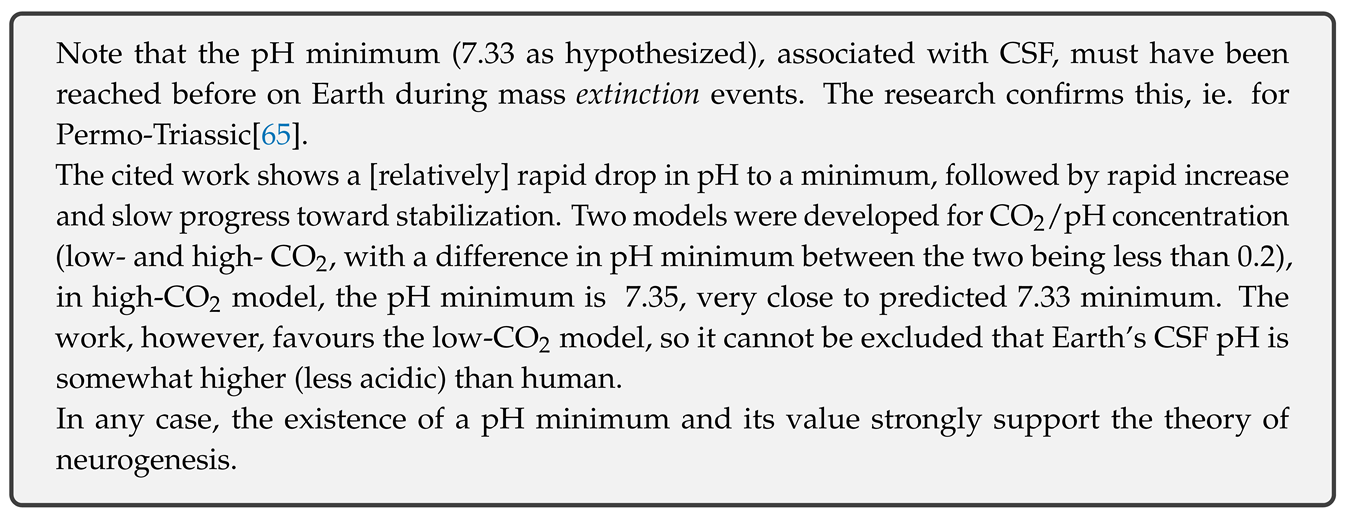
A precursor of 6 mantle layers has likely been created in events during Precambrian era, while population with neuron cells and final formation is occurring in Phanerozoic.
There have been 5 major extinctions in Phanerozoic, thus the next event should populate top layers and complete the formation of the final layer (I):
Formed layers of Earth’s brain are shown on Figure 17. Comparing with other layers, it seems evident that layer I is yet to be completed - green line shows possible seismic velocities after formation.
Energy from the Sun provides incubation energy used for the maintenance of the Earth’s surface ecosystem and weak evolution, but additional energy is needed for the formation of brain layers of homo.omega.

This energy is delivered through asteroid (also could be interpreted as food) and possibly cometary (water/organic compounds) impacts.
Year 2300 AD for the event is very conservative though, as it is based on linear extrapolation, does not include rising water temperatures and reaction of the biosphere.
Acidification of water at these events must be, in large part, driven by injections of gases (ie. sulfur dioxide) through oceanic ridges and vents which would introduce significant departure from linear correlation of pH with atmospheric CO.
Mathematical analysis of past perturbations of Earth’s carbon cycle [67] also predicts sooner triggering of the 6th major extinction event, before year 2100[68] (based on most likely future emission scenarios, the critical mass of oceanic carbon uptake calculated by the study author will be reached before year 2066).
From Figure 18 and more recent models [70], it is evident that CO concentration has a decreasing trend (expected due to increased energy from the Sun = less greenhouse gases needed to maintain the temperature).
Everything in nature oscillates (and fluctuates) so this decrease in amplitude should not be linear either, however some periodicity in extinctions must be present.
Statistically significant periodicity of extinctions[71] (at least in the last 250 million years) has been noted before - 26, and more recently, 27 million years between extinctions[72]. In any case, due to differences in extinction strength, multiple harmonics (or energy splitting of a single oscillator) are possible.
Using available data, one can construct models for atmospheric CO concentration synchronized with the oceanic pH minimum of a particular major extinction, as shown in Table 22.
Models are constructed in such a way to simulate oscillation of CO markers and compression of the amplitude with time, but they are also quantized - each marker is a multiple of 50 ppm CO quantum.
Some of the models are shown in Figure 19, blue dots are major extinction events, red triangles are minor extinction events (the curve does not necessarily follow actual CO levels between the extinctions, it is only used to illustrate oscillation of markers).
From these models, grouping of extinctions (suggesting oscillation of frequency) becomes more apparent. Major extinctions can be grouped into pairs separated by 126.5 (±8.5) million years, while paired extinctions are separated by roughly half that distance - 62.5 (±11.5) million years. Minor extinctions (420, 305, 145 and 34 mya) may be grouped in the same way - pairs separated by 160 million years, 113 (±2) million years separation of paired extinctions.
Model a) is the product of energy level splitting of a single oscillator, while b) is the product of 2 harmonic oscillators - one high energy (major) and one low energy (minor).
Points on the curve should not be interpreted as maximum atmospheric CO levels across the boundary, simply the points of migration or pH minimums.
While these particular models may be speculative, all Phanerozoic CO models show decreasing CO over time (this should be more evident when comparing boundaries of major extinction events) and recent research shows that maximum atmospheric CO across the K-Pg boundary (last major extinction) was 875 ppm[73].
Thus, the maximum atmospheric CO concentration during current extinction should be lower than 875 ppm, probably not higher than 800 ppm and likely lower than 800 ppm (suggesting that a larger part of acidification will not be sourced in dissolved atmospheric CO).
Recent history of CO concentration is shown in Figure 20. Assuming that CO has been, during that history, correlated with rate of evolution, one can extrapolate the relation for accelerated evolution of the current extinction.
Extrapolating from Figure 20, from year 1850 onward:
which, for the concentration of 800 ppmv gives year T = 2075.
While humans may eventually reduce their CO emissions significantly, the rate of evolution should keep accelerating according to equation and, regardless of atmospheric CO (which may still be increasing even with 0 human emissions), the required pH minimum will eventually be reached.
Asteroid impacts, previously correlated with Earth’s graviton energy level changes, should start before the migration, increasing in frequency and energy afterwards. Although required energy for changes may be lower than in previous major extinctions, it should still be significant.
Assuming interval between impacts is quantized proportionally to a 50 ppm CO increase (representing a quantum of energy), given the C1.1 equation, one can calculate years of impact and correlated these with possible impactors, as shown in Table 23. Evidently, there are good candidates among extinction causing asteroids in NEO (near Earth orbit) for calculated dates.
Fission of extinction pulses is possible (multiple impacts, ie. one in 2029 and other in 2066) and may be interpreted as splitting of energy levels (breaking of Apophis - homo induced?), which has probably happened in previous extinctions.
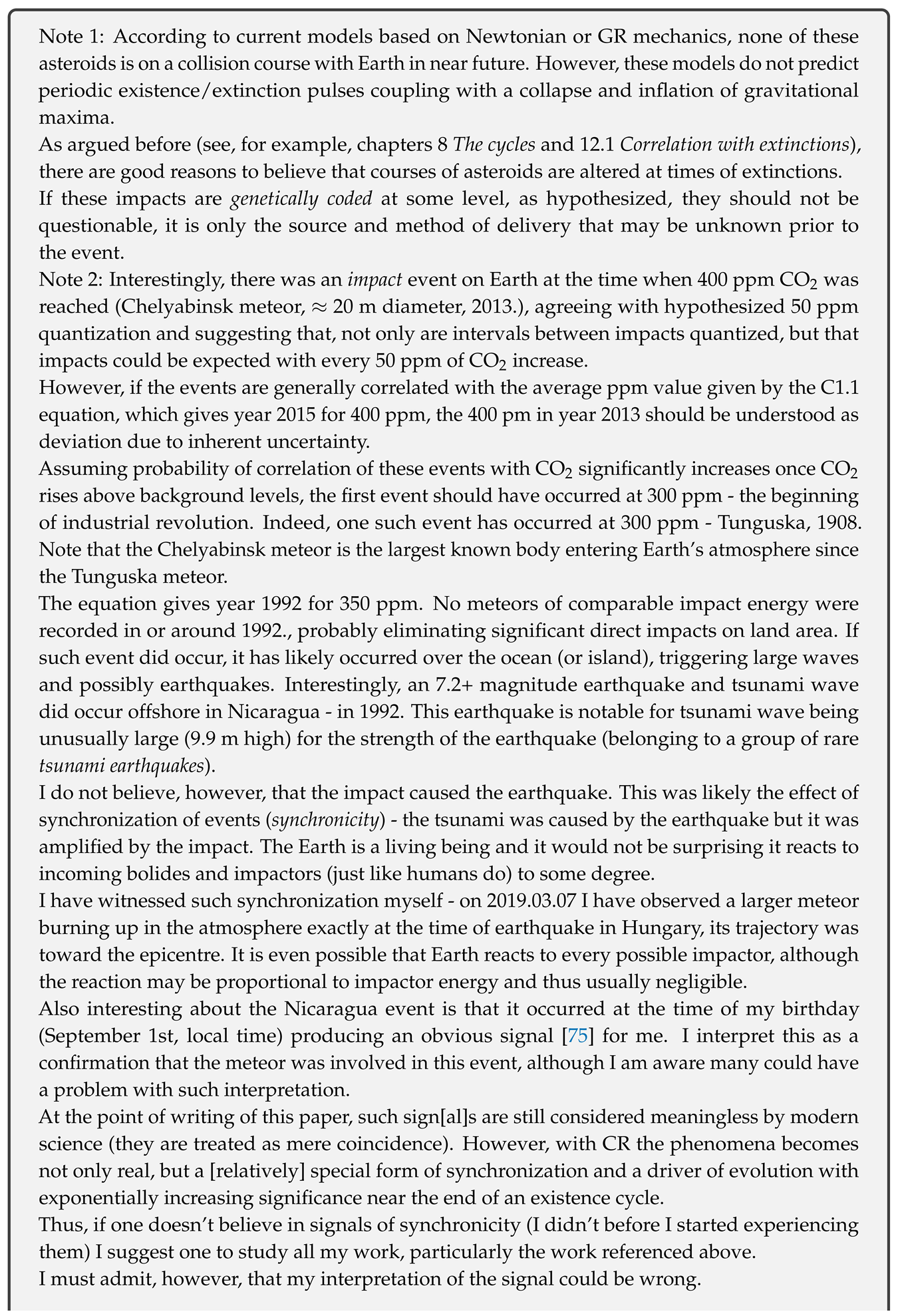
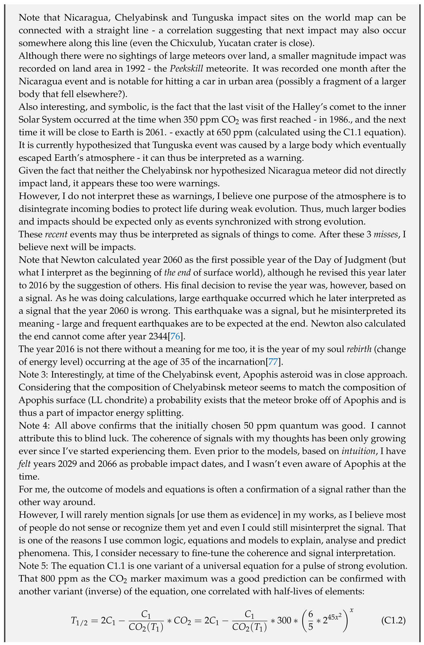
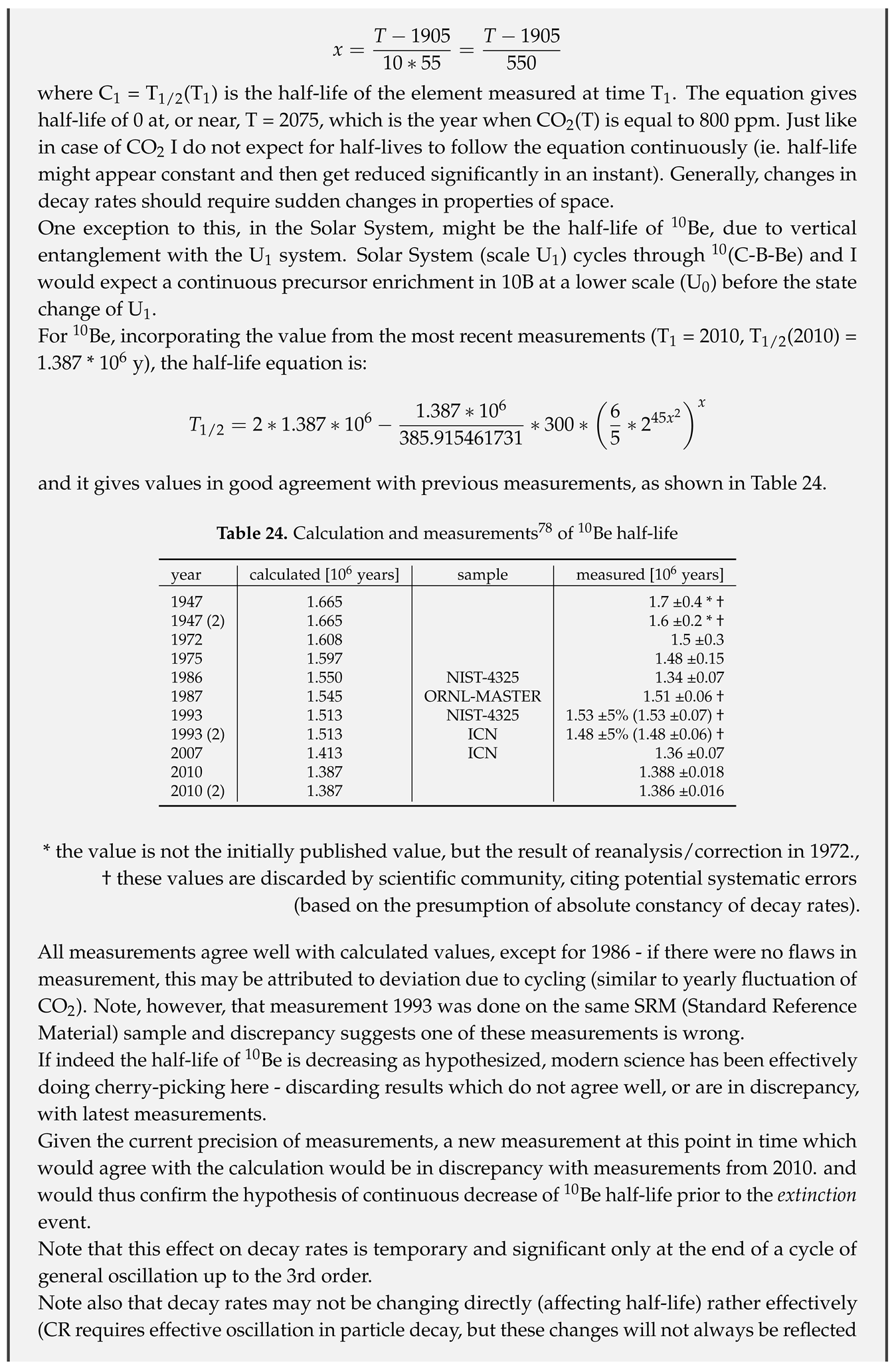
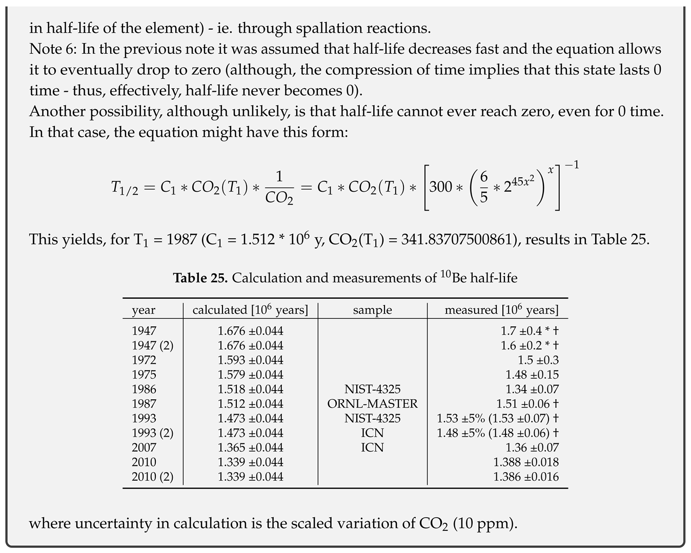
Such pulses might not only be plausible but necessary - first pulse would include asteroid impact(s) (possibly triggering additional ocean acidification and formation of the layer in the mantle), the other would provide new water/life, either by comets or asteroids. A third pulse in between might also be needed to trigger the (now acidified - CSF) ocean sink and, relatively, sterilize the surface (as noted before, all this is probably synchronized with magnetic field collapse, allowing surface sterilization by UV/gamma radiation).
It might seem that new water this time is not needed - as formation of mantle layers should be complete with this extinction (corresponding to Carbon nature of the Solar System) there is no need for cultivation of new progenitor cells on surface. However, it probably does happen as it would provide additional radiation protection and provide support for whatever life remains on, or near, surface.
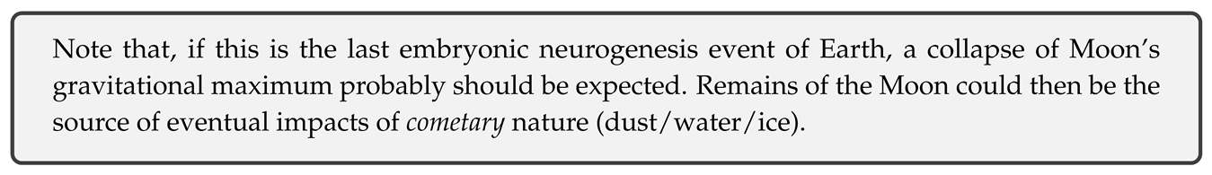
This is evident on Mars - as layers below the surface formed, magnetic field receded leaving the surface sterilized. Delivered water froze and is now covered with dust. Thus, one can only expect to find residual and resilient bacteria within the crust of Mars.
Similar happened on Venus except water evaporated due to high surface temperature.
Nothing in nature is linear (although this approximation may be suitable during stages of weak evolution) and in these extreme events one can expect significant departures from linear relations (by multiple orders of magnitude) between phenomena.
Since these events are coupled with gravitational stresses of the Solar System one can expect temporary but significant increase in alpha and neutrino radiation (radiation flux induced by temporary collapse of a gravitational well associated with a large scale graviton - strongly affecting half-lives of isotopes).
The assumption of absolutely constant decay rates will not only produce incorrect ages but can result in misplacement of events on a geological timescale. Thus, inconsistencies in certain geological records can serve as indirect evidence to disruptions in decay rates.
Consider the neutrino pulse on Figure 21 - under the assumption of constant decay rates, 3 different fossil records A, B, C may give following results:
- assuming non-isotropic space-time perturbation, such that fossil record A decay is not affected by the event at t, the event at t (associated with fossil record B) might appear to have happened before the event at t (associated with fossil record A)
- in case decay rates of both A and B are affected, the distance of t and t to t will be increased (time interval expansion)
Neutrino flux can also be decreased indicating shortening (rather than expansion) of time intervals, although in this context the increase of the flux is expected.
Due to accumulation, duration of fossilized events would apparently increase with time so older events would seem longer in duration compared to more recent events. This is exactly the case with current fossil evidence of past carbon cycle disruptions.
In such case, the current rate of CO injection is not different from those in previous major extinctions (the fact that it is anthropogenic makes no difference).
If one assumes that the average period between extinctions is equal to the 2nd order oscillation period of the Solar System, in case of ideal synchronization, it is quantized by the 3rd order period of existence (T = 1.512 * 10 years). In such case, assuming the period must be roughly 26 or 27 million years, the proper period is:
This is in agreement with previously determined periodicity of impact cratering (25.8±0.6 * 10 years)[72].
One can now assume that the CO injection within the Cretaceous-Paleogene (K-Pg) boundary (66.5 - 65.5 mya) is equal to current injection (currently dominantly anthropogenic) and that increase of decay rate (effective compression of time, causing boundary to be significantly overestimated in duration) is induced within the boundary - with the start of boundary corresponding to t and end to t on Figure 21.
Assuming CO increased from 780 ppmv to 1440 ppmv (CO = 660 ppmv) in period 66.5 mya - 65.5 mya (t = 1 million years)[81], compression of time t with each major extinction is:
where t is the period of 660 ppmv of anthropogenic CO increase since year 1850 (assuming this is the start of the new boundary), calculated using (C1.1).
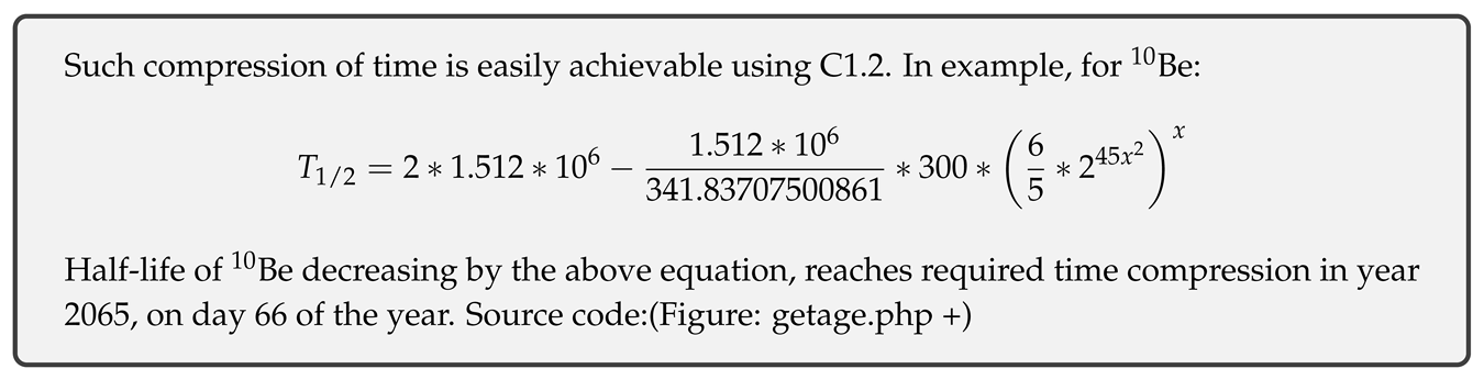
However, year 1850 as the start of the boundary is not convincing and recent research shows CO injection of 250 ppm, not 660 ppm, within the K-Pg boundary, though this does not affect compression (t) significantly (it makes it larger for a couple of decades at most).
Most likely start of a new boundary (end of Holocene) is year 2065 or 2066, which, with an increase of 250 ppm, gives year 2084 as the end, the same as in the previous assumption (1850 + 234 = 2084).
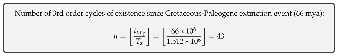
Gravitational collapses during strong evolution pulses with a period of T years (3rd order period) may last only t = 19.3 seconds, but collapses during stronger evolution pulses occurring with a period of T years (2nd order) last longer (possibly 7 days).
With each extinction, gravitational collapse of the Sun releases the pressure from condensed energy beyond the surface event horizon and the Sun effectively starts expanding.
The expansion reaches the orbit of Mars before the gravitational well is restored, so, assuming expansion at the speed of light, time of increased decay radiation is:
where r is the distance of Mars to Sun.
Now one can calculate time compression with each cycle (pulse) of existence t and each extinction t:
Age of Earth is thus overestimated by:
giving the real age of Earth:
where T = 4.54±0.05 * 10 years.
If one assumes that T is the equivalent of 1 day of human embryo development, Earth is at the week 25 (GW25) of gestation period (right at the beginning, in case of corrected age).
The GW25 marks the end of embryonic neurogenesis in humans and thus agrees with the suggestion of final major extinction.
The current carbon cycle disruption (6th major extinction) will thus not span thousands ( 10000) of years as predicted by the assumption of constant decay, but at most 234 years - starting from year 1850 (10000 years of already passed Holocene extinction may be regarded as a precursor to the major event starting at year 1850).
Note that this year corresponds to 950 ppm, as predicted by (C1.1).
14.4.1. Magnetic field collapse
As noted before, the 6th major extinction will likely include a decline of the Earth’s magnetic field, either as a temporary excursion (partial or global collapse), part of a complete reversal, or even a longer-lasting or permanent retreat. The Earth’s magnetic field is currently declining at an accelerated rate, which, when coupled with the rapid movement of magnetic poles, indeed suggests imminent collapse. The previously determined correlation of the 4th order period of general oscillation of the Solar System with past excursions (see chapter 8 The cycles) also suggests that, at least, a magnetic excursion is near.
If that is so, when will the collapse, partial or not, occur?
With no further acceleration of the decline the collapse would occur sometime beyond year 2100. However, such scenario is unlikely - additional acceleration is expected for a collapse.
The collapse should also be relatively synchronized with other impactful events, which, as I hypothesize, are correlated with the rate of evolution - which is currently correlated with the rate of atmospheric CO increase. With the assumption of events occurring with every 50 ppm increase of CO, per the equation C1.1, one obtains the following years:
- 2029, 2040, 2048, 2055, 2061, 2066, ...
Thus, the magnetic collapse should not occur before year 2029 (or, 450 ppm CO) and most likely not after year 2066. I find it likely to occur sometime around 2048, however, it full collapse is imminent, it may be preceded by multiple partial and/or temporary collapses, perhaps even with first one occurring 2030±1.
14.4.2. Sea level changes
Neurogenesis requires transfer of differentiated progenitor cells to subterranean world, into designated mantle layers. Therefore, a passageway must exist somewhere, connecting the surface with underground tunnels leading to such places - unless one is created when needed, which I find unlikely.
Scaling the largest neuron cells to Earth size, such passageway must have a radius of at least ≈ 250 meters to allow sequential cell transfer. However, parallel transfer of multiple cells is certainly more plausible - a radius on the order of 10 m.
Thus, the only location where this could remain hidden (protected) and isolated when unused is Antarctica. Ice melting is required to expose this location but likely also to rise the sea level in order to pick up the proteins and cells on land area.
Rise in atmospheric greenhouse gases is unlikely to produce adequate rise in temperature required to melt all ice in the predicted short time-frame. Thus, different mechanisms should be responsible to induce significant breaking and melting of ice sheets. In addition to greenhouse gases, volcanism/geothermal sources are likely. Melting can also be accelerated by asteroids, but also by alien species from the deep.
14.4.3. Analysis of past extinctions
Here, past extinctions are analysed for periodicity, with incorporated corrections by previously calculated time compression due to pulses of decay rate changes.
Periodicity is obtained using circular spectral analysis [83] of a couple of datasets, which all give similar results.
Data is grouped into energy levels corresponding to the extinction magnitude (5 - major extinctions, 4 - minor extinctions, 3 - other extinctions, 2 and 1 - potential extinctions).
The method In the circular model of periodicity a time line is wrapped around a circle, the circumference of which represents a trial period. For each occurrence, a unit vector from the origin is calculated. If periodic, the series will tend to form a cluster at one point on the circumference when the correct trial period is used. Here, angular location relative to 0 (present) gives the phase (t).
Ages of individual events (t) are transformed to angles (a, b) for each trial period P:
where R is a mean vector magnitude (normalized measure of goodness of fit). The phase shift (t) is calculated as follows:
Dataset 1 Extinction events in dataset 1, grouped into energy levels and calculated corrected ages for these events, respectively, are shown in Table 26.
Maximal R was obtained for a period P = 25.92 My (million years), with a phase of 9.355 My.
On the left, Figure 22 shows extinctions plotted against the obtained periodicity (dashed grey line), solid colored circles are extinction events with corrected ages, empty circles are extinctions with non-corrected ages. On the right, Figure 22 shows the result of circular spectral analysis.
Dataset 2 Here, a larger dataset from a single source was used. Maximal R reveals a period P = 26 My, with a phase of 8.617 My.
Table 27.
Extinction events dataset 2, source: Gradstein2016
| energy level | extinction events [mya] | extinction events (t), age corrected [mya] |
| 5 | 66, 201.4, 251.9, 372.2, 445.2 | 61.986, 190.308, 238.041, 352.461, 421.348 |
| 4 | 37.8, 145, 259.8, 306.7, 419.2 | 36.206, 136.774, 245.793, 289.975, 396.744 |
| 3 | 11.6, 93.9, 183.7, 228.5, 272.3, 423, 427.4, 485.4, 500.5 | 11.402, 88.465, 173.88, 215.987, 257.12, 400.469, 403.82, 458.929, 473.782 |
| 2 | 113.1, 168.3 | 107.344, 159.702 |
Extinctions and the result of spectral analysis are shown in Figure 23.
Dataset 3 Previous datasets do not take into account possible splitting of energy levels. Here, an even larger dataset is presented which shows possible energy splitting and how this, when not accounted for, causes lower confidence in calculated P.
Table 28.
Extinction events dataset 3, source: Gradstein2016
| energy level | extinction events [mya] | extinction events (t), age corrected [mya] |
| 5 | 66, 201.4, 251.9, 372.2, 445.2 | 61.986, 190.308, 238.041, 352.461, 421.348 |
| 4 | 37.8, 145, 259.8, 306.7, 419.2, 514 | 36.206, 136.774, 245.793, 289.975, 396.744, 486.084 |
| 3 | 11.6, 93.9, 183.7, 228.5, 272.3, 423, 427.4, 485.4, 500.5, 541 | 11.402, 88.465, 173.88, 215.987, 257.12, 400.469, 403.82, 458.929, 473.782, 511.664 |
| 2 | 113.1, 168.3, 330.9 | 107.344, 159.702, 312.804 |
| 1 | 295, 346.7, 393.3, 467.3 | 279.448, 328.357, 372.239, 442.101 |
Here, for R = 0.413, obtained P = 22.493 My, phase 15.603 My.
Dataset 4 Here I hypothesize that deviations from P are the result of energy splitting into smaller events which when grouped properly would fit on P intervals.
The dataset is the same as dataset 3, except the hypothesized splittings (circled extinction pairs in Figure 24) have been grouped into a single event, simply by using arithmetic mean age of the pair.
Table 29.
Extinction events dataset 4
| energy level | extinction events [mya] | extinction events (t), age corrected [mya] |
| 5 | 66, 201.4, (251.9+259.8)/2 = 255.9, 372.2, 445.2 | 61.986, 190.308, 241.967, 352.461, 421.348 |
| 4 | 37.8, 145, 306.7, (419.2+423)/2 = 421.1, (514+541)/2 = 527.5 | 36.206, 136.774, 289.975, 398.619, 499.361 |
| 3 | 11.6, 93.9, (183.7+168.3)/2 = 176, 228.5, (272.3+295)/2 = 283.7, 427.4, (485.4+467.3)/2 = 476.4, 500.5 | 11.402, 88.465, 166.304, 215.987, 268.346, 403.82, 451.053, 473.782 |
| 2 | 113.1, (330.9+346.7)/2 = 339 | 107.344, 320.78 |
| 1 | 393.3 | 372.239 |
Figure 24.
Extinctions
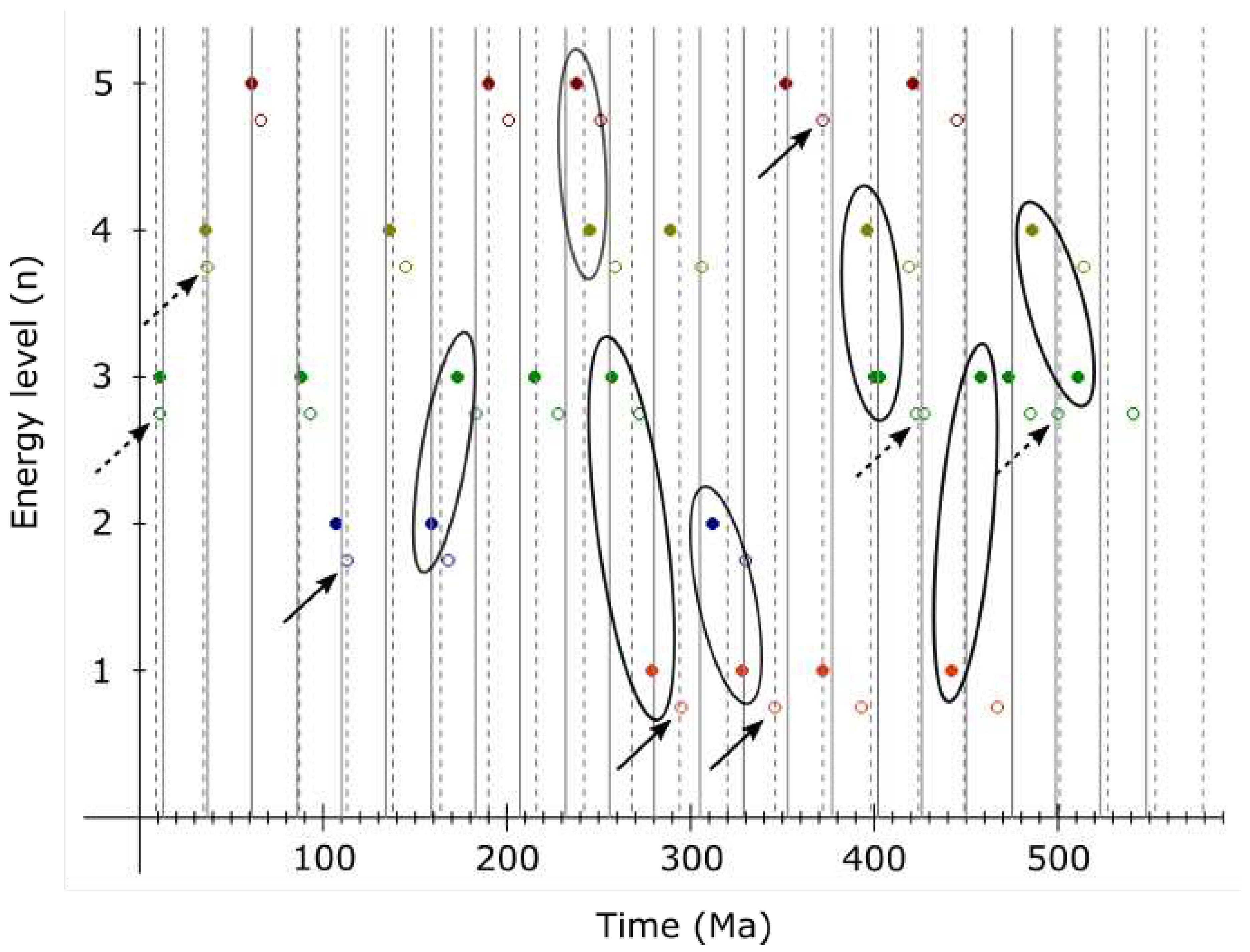
Figure 25.
Extinctions (left), spectral analysis (right)
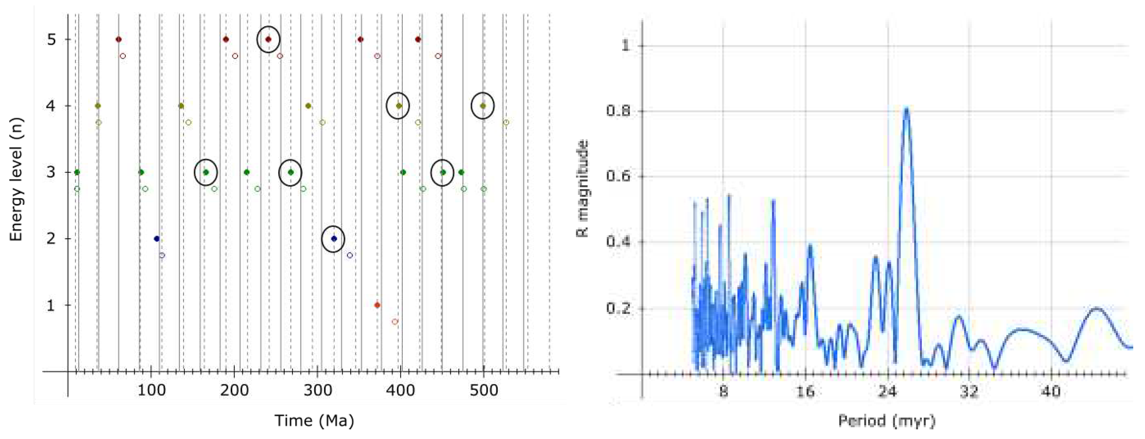
The R peaks at 0.807, corresponding to P = 25.89 My, very close to one obtained from dataset 1. Phase is 9.55 My.
Dataset 5 Here dataset 4 is modified with the assumption that splitting occurs in all events, thus, in addition to previously grouped events, the remaining non-grouped events have been grouped with adjacent boundaries.
Table 30.
Extinction events dataset 5
| energy level | extinction events [mya] | extinction events (t), age corrected [mya] |
| 5 | (61.6+66)/2 = 63.8, (199.4+201.4)/2 = 200.4, (251.9+259.8)/2 = 255.9, (372.2+382.7)/2 = 377.5, (443.8+445.2)/2 = 444.5 | 60.81, 189.333, 241.967, 356.687, 420.648 |
| 4 | (33.9+38)/2 = 36, (139.4+145)/2 = 142.2, (306.7+314.6)/2 = 310.7, (419.2+423)/2 = 421.1, (514+541)/2 = 527.5 | 34.431, 134.998, 293.926, 398.619, 499.361 |
| 3 | (11.6+13.8)/2 = 12.7, (89.8+93.9)/2 = 91.9, (183.7+168.3)/2 = 176, (228.5+237)/2 = 232.8, (272.3+295)/2 = 283.7, (427.4+430.5)/2 = 429, (485.4+467.3)/2 = 476.4, (497+500.5)/2 = 498.8 | 12.502, 86.49, 166.304, 220.213, 268.346, 405.395, 451.053, 472.107 |
| 2 | (113.1+126.3)/2 = 119.7, (330.9+346.7)/2 = 339 | 112.87, 320.58 |
| 1 | (387.7+393.3)/2 = 390.5 | 369.489 |
Figure 26.
Dataset 5, spectral analysis
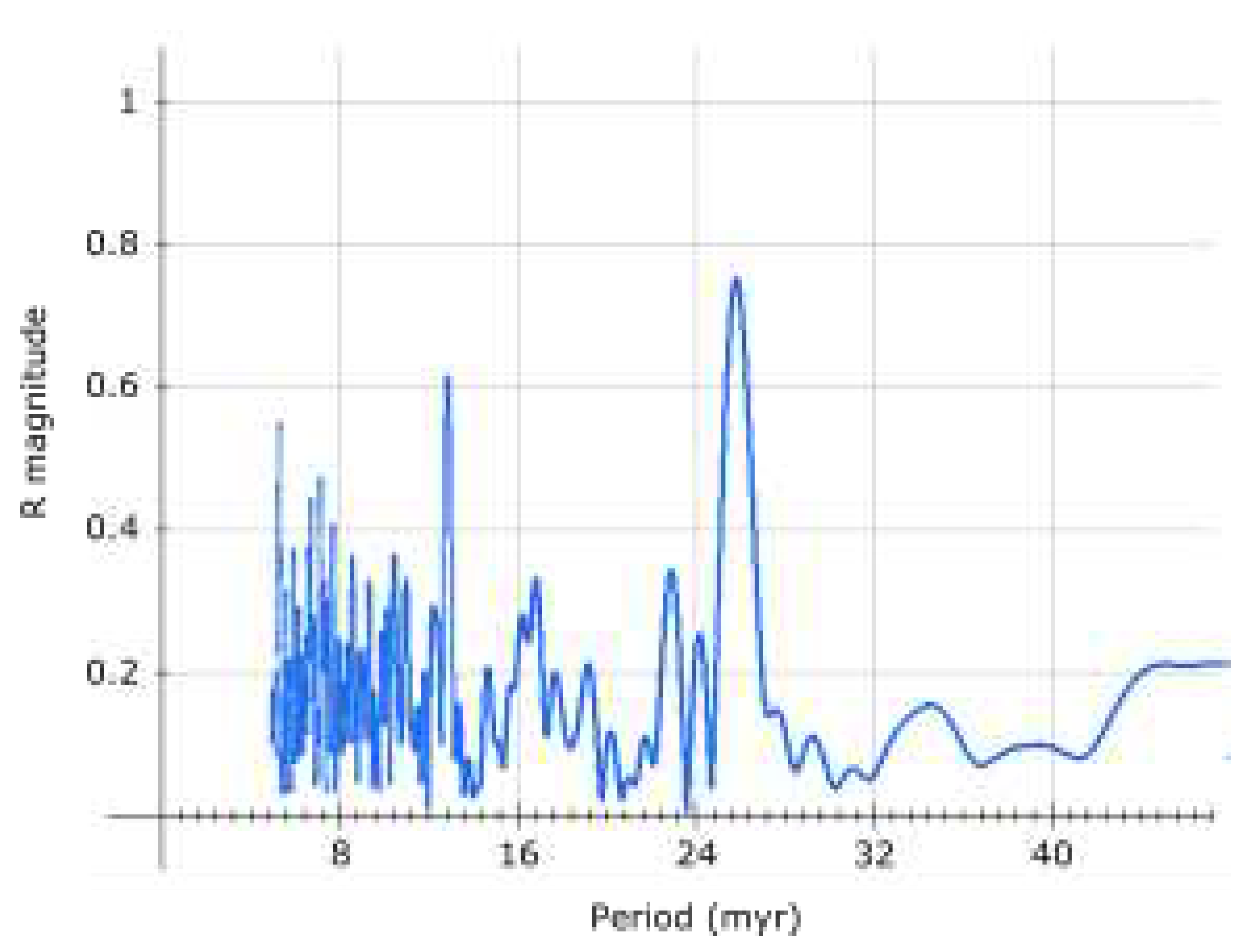
The R peaks at 0.75, corresponding to P = 25.84 My. Phase for this P is 9.78 My, however, here another peak at 12.875 My (R = 0.61) reveals a likely harmonic.
Dataset 6 Here, dataset contains only highest energy (major and minor) extinctions, from dataset 1. This dataset gives highest R maximum (0.837), a period P = 25.74 My, with a phase of 9.689 My.
Table 31.
Extinction events dataset 6
| energy level | extinction events [mya] | extinction events (t), age corrected [mya] |
| 5 | 66, 201.3, 252.2, 365, 445 | 61.986, 190.208, 238.316, 345.385, 421.148 |
| 4 | 37.8, 145, 260, 305, 420 | 36.206, 136.774, 245.993, 288.3, 397.519 |
Confidence Note that equal weight was assumed for all extinctions in a particular dataset. Different weights can affect the confidence in the result (less if they are all harmonics). But even with that taken into account, there is high confidence in P ≈ 25.74 My - 25.89 My.
The result with highest confidence (25.74 My) is also the closest to calculated ideal quantization by the 3rd order period (1.512 * 10 My) - 25.704 My, further increasing confidence in such periodicity.
Note that the burning cycle of the Sun’s core is calculated (in the "Quantization of the Sun" chapter) to be equal to 25.746608 My, confirming the signal.
Neurogenesis in standard lifeforms on Earth during embryonic development does imply certain periodicity in the formation of brain layers and neuron migration.
High energy impact cratering and extinctions (migrations) in planetary neurogenesis should be no exception.
In fact, with such periodicity and the last high energy extinction 37.8 My in the past, next one is overdue, roughly by the phase shift.
Thus, imminent major extinction as calculated using models based on C1.1 equation should not be surprising.
Supplement Here is the code used to calculate correct ages of extinction events, perform the analysis and generate images.(Figure: getext.php +)
14.4.4. Correlation with mantle layers
Grouping and correlation of extinction events with the formation of brain [mantle] layers also indicates that another major mass extinction should be near, at least in geological terms.
This correlation is shown on Figure 27 - time between major extinction events of Phanerozoic is proportional to thickness of a corresponding mantle layer.
This is, effectively, a conversion of time separated discontinuities into events separated in space.
To quantify the correlation, periods of weak evolution and thicknesses of mantle layers have been normalized:
Results are shown in Table 32. Here, corrected extinction ages are used, although non-corrected ages would yield similar results. Correlation in absolute value varies between the pairs, but overall, it is apparent.
At least some discrepancy could be explained by the fact that formation is not yet complete - ie. the boundary between layers 3 and 4 might change with the pending extinction.
If layer 3 decrease would be equal to layer 4 increase (≈ 0.0575 in normalized value) and layer 1 decrease to layer 2 increase (≈ 0.0275 ≈ 0.0575 / 2), with a small decrease in layer 5 (0.013 ≈ 0.0275 / 2) coupled with equivalent increase in layer 6, normalized extinction and mantle boundaries would be almost equal.
Effectively, what is necessary for better agreement is the upward movement of 3 discontinuities (between layers I and II, III and IV, V and VI).
However, exact location of boundaries is a matter of debate. They must have some thickness, so it may be more appropriate to equate layer thickness with distance between discontinuities. If that would be a distance between lower discontinuities of two boundaries, it would, for layer 1, yield a normalized value exactly equal to the corresponding normalized period of weak evolution:
Also, globally average velocities might not be the best choice for determination of layer discontinuities - ie. Lehmann discontinuity is at 220 km for tectonic North America, but 200 km for shield North America [96], while it may be absent beneath north Atlantic and other oceans.
If one assumes that 200 km is a proper boundary (220 km may be a precursor boundary that will reduce to 200 km with complete formation), the correlation with extinctions for both layers, I and II, becomes remarkable:
Some report the base of the upper mantle at 670 km[97] rather than 660, this improves the correlation with layers 5 and 4:
Now, the only problematic boundary is the one between layers 3 and 4 (at 520 km). Some do report this boundary at 500 km, which gives much better agreement:
Note that extinction boundaries also have some thickness or uncertainties, notably first three, which may explain differences in reported discontinuity depths. The 3rd major extinction (Permian) is apparently split into two events (End-Capitanian and Permian-Triassic). Using End-Capitanian 245.793 Mya (259.8 Mya non-corrected) instead of Permian-Triassic 238.041 Mya (251.9 Mya non-corrected) as the date of Permian extinction gives results in remarkable agreement with the obtained layers 3 and 4 (with discontinuities at 410 km, 500 km and 670 km):
The correlation, with above adjustments, is shown in Table 33 (with ages rounded to a single decimal). The correlation, using uncorrected ages for major mass extinctions, is shown in Table 34.
The excellent agreement here suggests no further adjustment of discontinuities is needed, except possibly for layer I, as shown in green in Figure 27 (right) which should be unsurprising given the correlation with the current extinction.
Correlation of layer 6 and the corresponding period of weak evolution has not been determined due to unknown boundary.
However, assuming the extinction at the start of Phanerozoic (511.664 mya in corrected age, or 541 mya non-corrected) is correlated with the lower boundary of layer 6, one can calculate the thickness of layer 6:
In that case, a discontinuity, if formed, should exist in Earth’s mantle at a depth of 937 km (assuming boundary between layer 5 and 6 at 780 km).
Apparently, this discontinuity has been detected[98] (at 940 km).
14.4.5. Evidence in time compression
If planetary neurogenesis is happening on Earth, it was likely happening on Mars and Venus too. Time, however, flows differently for animals of different size. The rate of evolution on Mars should then be different from the rate of evolution on Earth - it should be faster.
Applying Kleiber’s law, 4.54 billion years of evolution on Earth would, on Mars, last:
M = 0.642 * 10 kg
M = 5.972 * 10 kg
T = 4.54 * 10 years
Assuming Mars was formed roughly at the same time as Earth, present time on Earth corresponds to a time 3.69 billion years ago on Mars (4.54 - 0.85 = 3.69).
This is a very interesting result as studies show that Martian climate shifted from habitable to uninhabitable - when its atmosphere was lost and liquid water disappeared from surface, roughly 3.6 billion years ago[99] (src[100]).
This suggests that current major extinction on Earth may indeed be the final major extinction of the planetary embryogenesis (neurogenesis), after which the Earth’s surface will become permanently uninhabitable (although periodic and possibly spatially limited pulses of habitability cannot be excluded, as hypothesized pulses of adult neurogenesis).
The same equation gives evolution period of 3.9 billion years for Venus, suggesting Venus lost habitability some 640 million years ago. Again interesting, as studies show that Venus did lose habitability roughly 700 million years ago[101].
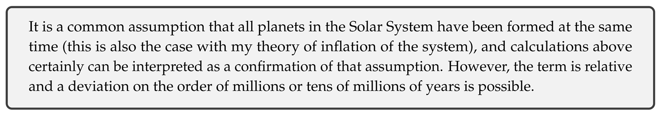
14.4.6. Some additional predictions of neurogenesis
If cultivation of life on planet’s surface is equivalent to cultivation of neural cells during embryonic neurogenesis in mammals, the events hypothesized above are not the only upcoming events that can be predicted.
Obviously, cultivation of cells/proteins must be limited. The most effective (or most energy efficient) way to limit population growth is to substantially decrease its fertility. Recent studies show that fertility in humans is indeed decreasing, at an accelerating pace[102].
Accelerated evolution likely includes accelerated ageing in some species or sub-species (in some, possibly reversed), cases of which are showing up in studies too[103].
14.5. Metabolism of Earth
Transfer of energy in wild flora and fauna is generally balanced both horizontally and vertically.
Vertical transfer of energy is a part of metabolism but changes in horizontal current affect the vertical transfer too (and vice versa).
Humans dominate in both horizontal (surface to surface) and vertical (Sun - Earth interior) energy distribution and transformation, disrupting the harmonics of life.
Horizontal effect is the increasing number of individuals at the cost of decreasing number and diversity of other species, while vertically it is the unsustainable exploitation of radiated and stored resources of the Sun/Earth ecosystem.
Thus, one may interpret humans as the metabolism energy carrier particles, in a limited domain.
With a human population N of 7.674 * 10, average mass m of 62 kg, and average lifetime t of 72.6 years (data for year 2019, except mass - 2012):
where M is the mass of Earth (5.9723 * 10 kg).
This gives a value of 0.756 for exponent, in agreement with Kleiber’s law.
However, in case of organ interpretation, the exponent suggests a superposition of a brain and a kidney.

In order for this superposition to differentiate into the brain, the exponent would have to reduce to 0.7.
There are several ways to achieve that (sorted by probability, from highest to lowest):
- increasing human lifetime (≈25 times) to 1813 years,
- reducing population (≈25 times) to 307243423,
- reducing mass (≈25 times),
- increasing Earth’s mass ≈100 times (≈ mass of Saturn).
If humans are indeed precursor proteins of neuron proteins of Earth, as carriers of energy of its brain metabolism, I would expect the solution to be a weighted superposition of the above.
However, if Earth has a heart equivalent (core), most likely it also has a kidney equivalent and the population might differentiate into proteins of varying function.
I, strive for neutrality - the equal, balanced usage of all parts of my universe. I am aware though, that this is an unreachable singularity, but it is the journey that makes one alive - for without it there would be no senses, for a sense of reason, and a reason for existence.
14.5.1. Nature of human cells
Dominance of lifeforms changes over time. At present time, homo species occupies and controls most of the surface of the planet. Human population is rising and thriving at the expense of other species.
While the dominion of species may be related to precursor nature of vital organism components, its behavior can be corrupted, so cultivation of new proteins becomes evolution of disease rather of something integral for survival.
While it is not questionable whether human species is a disease for the planet, it is questionable whether this is fatal or rather a normal part of evolution of healthy cells and proteins with self-correcting mechanisms.
Dividing the total surface area of Earth (R = 6371 * 10 m) with the number of people, one gets the maximum size of the cell:
Radius of space per person is:
If the radius of a human occupied cell of Earth is the mean free path r, the radius of a cell equivalent in human body of average diameter (height) h = 1.7 m is:
If one calculates using landmass only (people don’t naturally live on water):
Taking into account space used by wild flora and fauna:
This is in the range of a typical cancer cell. It is, of course, in the range of healthy cells too, but human cells are far from healthy.
It might seem that the radius r (r) changes with population, but this is not the case - if human space decreases, the space of wild flora and fauna increases and vice versa, thus it generally evolves weakly, remaining almost constant.
Figure 30 illustrates a homo cell on Earth’s surface, circled space (red) is occupied by a human and domesticated flora and fauna, other (green) by wild flora and fauna.
Figure 30.
Homo.beta cell
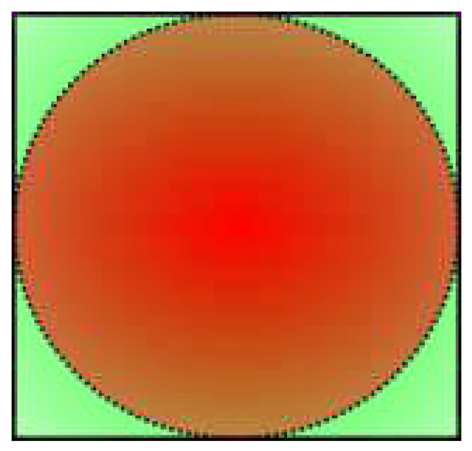
Figure 31 illustrates what I would consider a normal (healthy) unit of space on Earth. Red is a cell of homo.sapiens (Earth’s neuron cell), black lines are mental connections (synapses) to other cells.
Figure 31.
Normal cells
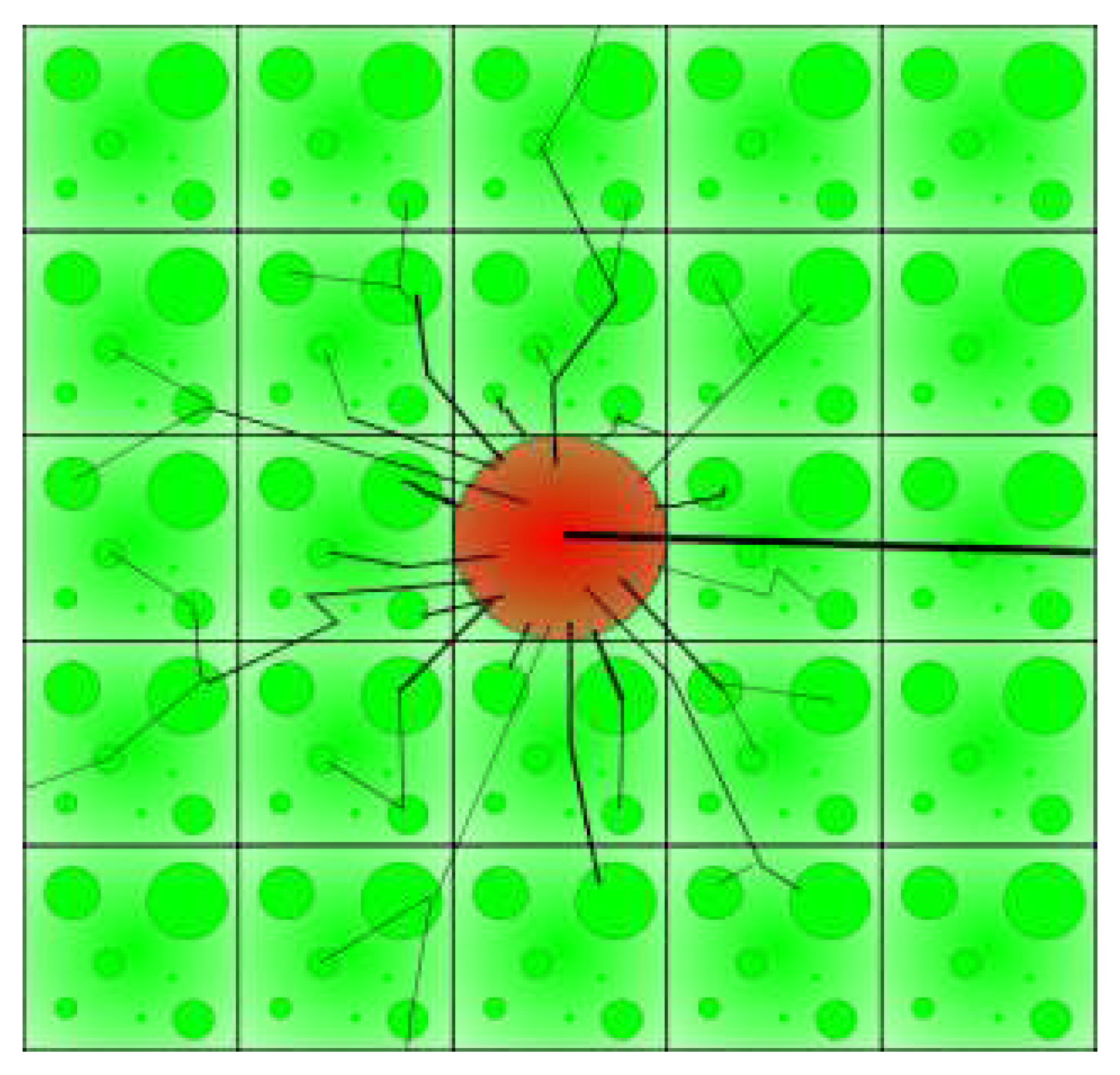
Figure 32 illustrates the cancerous, or current typical, unit of space on Earth. Blue and red are polarized human (cancer) cells.
Figure 32.
Cancer cells
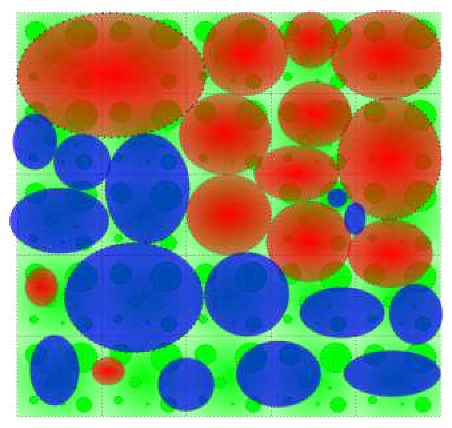
Figure 33 illustrates the outcome - death.
Figure 33.
Dead space
Cancer cell contains the individuals (proteins) and space affected by cancerous population, but one can even calculate the role of a human in the cancer cell:
This is in the range of a TGF- protein, a key player in cancer development.
Confirmation of this comes from recent studies[104], revealing human nature of TGF-:
"And while it may be difficult to imagine a protein with two dramatically different faces, it may be even more difficult to contemplate cancer cells exhibiting traits, such as cunning and deception. But the research underway at the University of Basel, and collaborating laboratories, has revealed that TGF- not only is a two-faced protein, it also is one that seems almost Machiavellian in its activities."[105]
Cancerous TGF- suppresses the immune response and prevents old cells/proteins from dying (regenerating). Humanity is, at the time of this writing, expressing this cancerous behavior on many levels:
- through treatment of diseases (including cancer) humanity is suppressing the immune system of Earth,
- forcing human life at all costs and treating death (as a disease) - instead of letting cells (and proteins - people/animals) die as programmed so they can regenerate,
- treating Earth and other life forms (and, generally, even people) as resources - instead of living in a sustainable symbiotic relationship,
- creating and living in centralized, stressful environments, promoting inequality in wealth and health,
- denying the truth.

The average cell cycle period of eukaryotic cell is T = 14.5 hours, scaled to Earth size, it is:
where T is the period of 3rd order existence cycle of Earth (1.512 * 10 years).
15. Quantization of Moon orbits
If gravity of the Earth’s [major] gravitational maximum is, as hypothesized, equal (or was initially equal) to surface gravity of the Sun, one would expect for orbitals of natural moons of Earth to be scaled orbitals of inner planets.
Allowed orbitals are thus:
where r is the Earth’s gravitational maximum radius (= inner core radius), R is the radius of the Sun and r is the orbital radius of a corresponding planet.
Using R = 695735 km, r = 1206.115 km, one obtains orbitals shown in Table 35. Evidently, the Moon is currently at the scaled Mars’ orbit. Even the distance between perihelion and aphelion is scaled by equal orders of magnitude - for Mars it is 42.61 * 10 km, while for the Moon, the distance is 42.2 * 10 km.
Small deviations from calculated values should be attributed to oscillation and phase shift in synchronization.
16. Quantization of the Sun
During inflation of the Sun, multiple gravitational maxima were inflating within. Collapse of these maxima as the Sun was deflating was fossilized in the Sun, in the form of discontinuities. As these maxima are now gravitational maxima of inner planets, entanglement exists between radii of discontinuities and planetary orbits.
Some discontinuities are strong (permanent) while some are weak, evolve over time and may periodically disappear. Apparent discontinuities are those between the core, radiative and convective zone, surface discontinuity and the boundaries of tachocline.
Regardless of current configuration (1e or 2e), each inner planet probably formed with the collapse of two maxima. Thus, each is entangled with 2 discontinuities in the Sun.
Initial inflation of planetary maxima must have been faster than light to preserve invariance.
If one assumes that all maxima initially had the mass of the Sun and energy density remained constant during inflation, with the collapse (energy level change) occurring once escape velocity was equal to the speed of light (in CR, discontinuities between energy levels are speed limits), orbital radii of planets become fossils of Schwarzschild radii:
R = initial radius
M = 1.988500 * 10 kg
c = standard speed of light = 2.99792458 * 10 m/s
G = 6.674 * 10 m/kgs
With equal escape velocity (pressure per surface quantum) between maxima (note that a smaller maximum is inside the other), radius of fusion of two maxima becomes the arithmetic mean of two radii:
In that case, discontinuities entangled with planetary orbits are at 1/5 R, 2/5 R, 1/2 R, 2/3 R and 1 R. Correlation of orbital and Schwarzschild radii is shown in Table 36, where R is the radius of the Sun (695700 km).
Significant orbital eccentricity of Mercury and Mars also seems correlated with Sun’s discontinuities.
If Sun’s core radius oscillates between 0.1 + 0.186 R = 0.286 R (previously hypothesized initial radius) and 1/5 R (current radius), with constant energy density between the two radii, time independent core radius [as superposition of two oscillatory states] is at 1/4 R.
This is correlated with Mercury’s orbit, as its distance from the Sun is at 1/4 MAU, while its perihelion is at 1/5 MAU.
According to equation S1.1 describing rotational velocities of plasma, and the actual velocity curve, significant points are at 0.1 R, ≈1/2 R, 1 + 0.18686 R = 1.18686 R and 32.8 R (0.1 MAU, half of Mercury’s perihelion).
The aphelion of Mars is at 1 + 0.18686/2 MAU = 1.09343 MAU = 249.2 * 10 m.
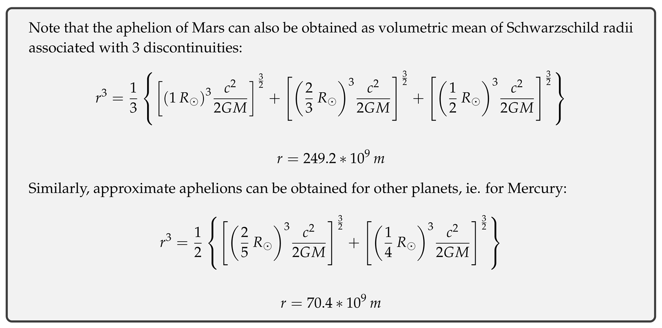
16.1. Layers of the Sun
Internal gravity of the Sun depends on the location of maxima and acquired real mass.
Distribution of mass, however, should not be complex unless there are collapsed large scale maxima inside. In any case, matter accumulated between two maxima should, in equilibrium, imitate a maximum and can thus be approximated as one (induced maximum).
One way to obtain gravity of a primordial Sun is to derive it from rotation of real mass - assuming greater rotation with greater gravitational mass, down to the inner core radius r, quantization is 1-dimensional:
Giving the scaled h constant:
Another way is to assume a completely naked Sun, in which case gravity from the surface down to the core is:
Gravitational profile of the primordial Sun (not taking into account the gravity of inner core maximum) is given in Table 37. Here matter velocity (v) is extrapolated from measurements, while space (Keplerian) velocity (v) is calculated from gravity:
Note that multiplying any discontinuity radius with inner core velocity v gives values proportional to r/R ratio and gives integer gravity (g) for inner core and all layers above.

Difference between current surface gravity and g is roughly equal to the sum of surface gravities of inner and outer planets:
thus, some entanglement might exist there too.
Below the gravitational minimum at inner core (r), quantization is 3-dimensional and gravity should be increasing until the next maximum:
16.1.1. Current G model
Unlike in space above the outer maximum, where gravity falls to zero effectively at infinity (due to next maximum being extremely far), below the maximum gravity falls to zero at finite distance due to compression of space.
With no inner maxima, the single point of zero gravity would be at the centre, however, due to relativity, inner maxima must exist (each inner maximum must also be a relative outer maximum).
If the radius of the outer maximum of the Sun is the surface radius, gravity should thus be decreasing below the surface to the point where it is cancelled by the [next] inner maximum.
Without the inner maximum, any free-falling real mass would be concentrated around the surface maximum. With inner maxima, concentration of real mass begins at the centre.
However, as each inner maximum has lower capacity than its outer maximum, greatest density of real mass will not be at the centre. Once inner maximum is at full capacity, as real mass accumulates between the inner maximum and the outer maximum, its counteracting the gravity of the outer maximum.
In equilibrium thus, greatest density of real mass is not at the outer maximum, rather between the inner and outer maximum.
This is shown on Figure 28. Here, dark matter gravity provided by [img] gravitational maxima is represented by solid black lines, while real gravity provided by real mass and its induced (effective) maximum is represented by dashed black lines. In case of outer maximum, grey line represents gravity with no real mass acquired (naked maximum), while for inner maximum, it represents the initial core maximum. Red dashed lines show linearly approximated density of real mass.
Figure 28.
Gravity of the Sun
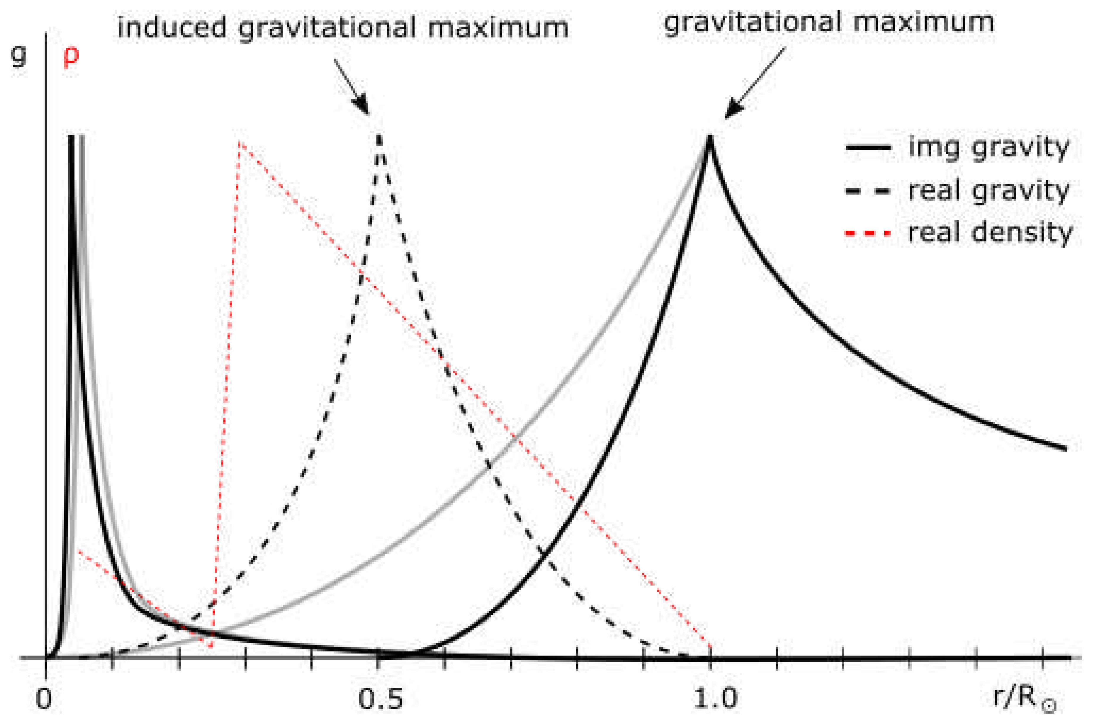
From Figure 28 one can extrapolate discontinuity candidates (r/R): 0.0385 ≈ 2/5 * 1/10, 2/3 * 1/10 (initial core maximum), 1/5, 1/4, 0.286, 1/2, 2/3, 3/4, 1.
In addition to these, there are other candidates, representing maximum deviation from these values - ie. discarding CMB relative relativistic energy, rest surface maximum is at 0.94 R.
16.2. Energy replenishment
Primary energy source of the Sun is, most likely, fusion.
Fuel for fusion must either be the real mass of the Sun (accumulated matter) or matter created through conversion of imaginary mass (dark gravitational potential) to real mass by some unknown mechanism.
In case of such conversion it would take tens of billions of years to spend all fuel.
However, this solution implies the Sun is eating itself and is highly unlikely.
The Sun is thus, most likely, burning its real mass which was accumulated most likely during inflation of its maxima (whether through inflation of smaller maxima or acquisition of matter by increasing vacuum pressure on U scale).
To determine how much fuel the Sun has left it is necessary to determine how much fuel it had at the beginning and the rate of fuel consumption.
Assuming fusion reaction 4H -> He (energy per reaction E = 4.32 * 10 J) and power output P of 3.8 * 10 J/s, time needed to spend all fusion fuel is:
m = available mass
m = proton mass
E = energy per reaction
P = power output
N = fraction of mass used in fusion
Since the Sun has two [major] maxima, fusion may be occurring at two places - in the core and above the core.
Gravitational mass of the surface maximum is assumed to be 1.988500 * 10 kg (or half that value at full capacity in case of interpretation with no mass shielding), while the gravitational mass of the core has been calculated previously to be 2.951797 * 10 kg.
Assuming that the calculated core mass is the mass of the maximum and therefore equal to the internal capacity for real mass, this capacity in equilibrium should be full and, due to mass loss (ie. through radiation), excess real mass must be constantly (cyclically) consumed as fuel.
It has also been hypothesized that the ratio of core mass and surface mass should be correlated with the ratio of mass between inner and outer planets.
Assuming that at the beginning of the core feeding cycle, these ratios are equal, fuel mass is the excess mass in the outer core corresponding to the ratio.
In case of thermonuclear fusion and with 2/3 of mass consumed, time needed for the core to spend all fuel is:
where m = 8.90211033 * 10 kg is the previously calculated initial mass of the core.
Assuming that, at the start of consumption cycle, imaginary mass (gravitational maximum) grows to initial mass radius (0.286 R) and decreases with energy loss, time left (assuming constant rate of consumption) before the next feeding cycle is then:
Negative time may be interpreted as the next cycle being overdue (core spent all fuel 838k years ago and is currently burning constitutional mass), or, that more than 2/3 of mass must be consumed in fusion.
In case 70% of mass may be spent:
However, as stated already, thermonuclear fusion in the core is unlikely. In case there is no fusion in the core at all, ruling out standard chemical reactions and radioactivity, the remaining possibility is heat generation through gravitational (Kelvin–Helmholtz) contraction:
M = initial core mass = 8.90211033 * 10 kg
R = initial core radius = 0.286R = 198970200 m
assuming logarithmic relationship between mass and radius contraction, the contraction may be approximated from the rate of Jupiter contraction:
M = Jupiter mass = 1.89819 * 10 kg
R = Jupiter radius = 71492000 m
dR/dt = rate of Jupiter contraction = -3.17 * 10 m/s
giving energy radiation of:
and time to spend all fuel:
M = current core mass = 2.951797 * 10 kg
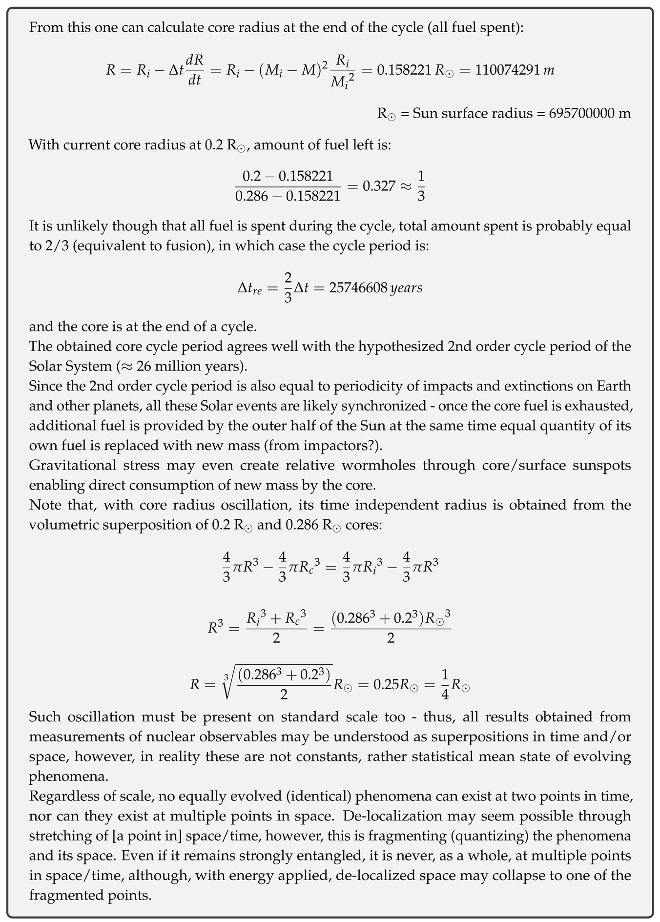
Unlike the core, the outer part of the Sun is most likely powered by fusion.
However, it too must have constitutional mass and fuel mass fraction of real mass (excess mass).
Most likely, fuel mass is equal to the previously calculated relativistic energy (CMB relative) of the Sun. In that case, time to spend the fuel is:
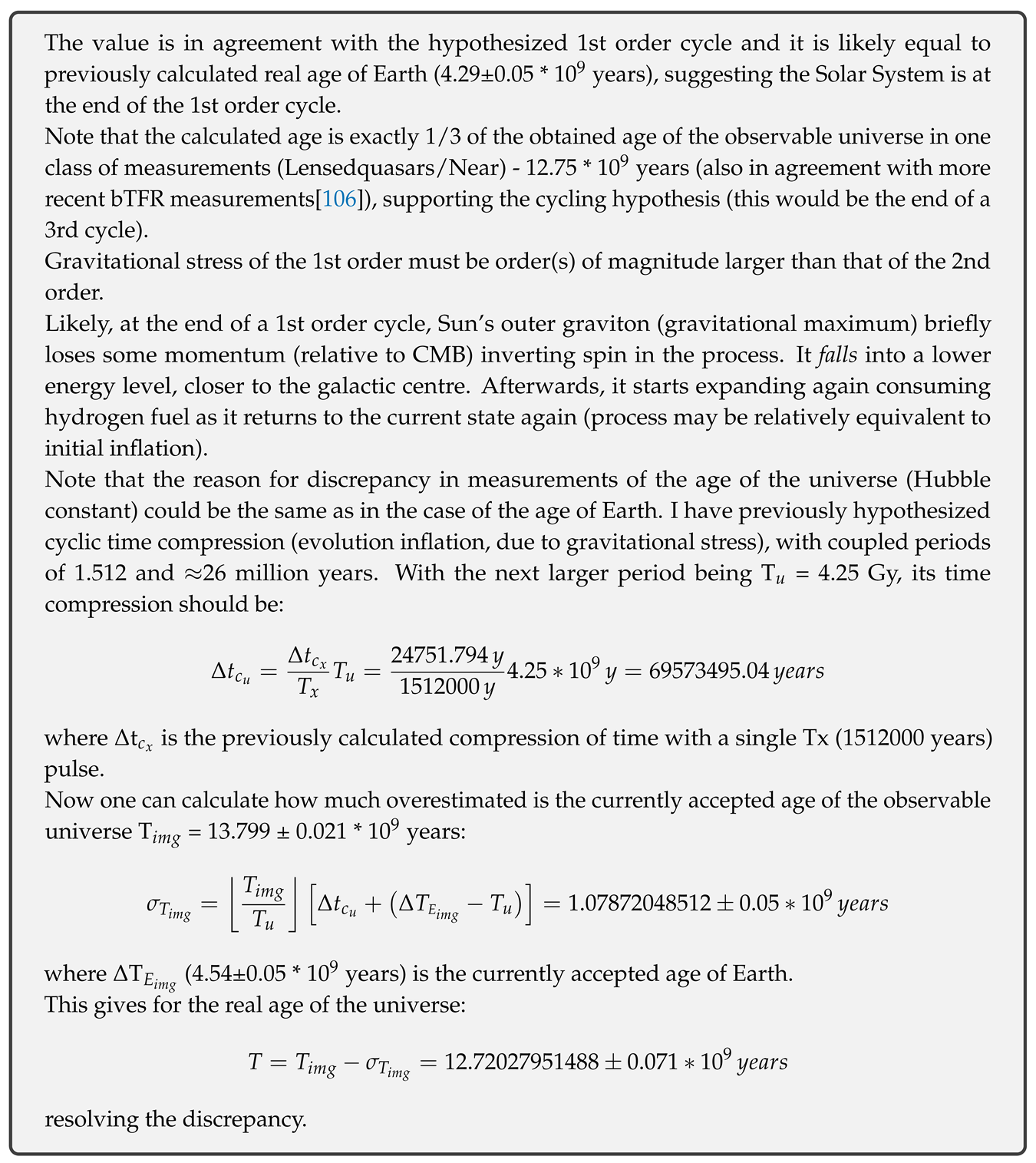
Another interesting solution is obtained if the fuel amount is equal to real mass of the Sun calculated with the assumption of, across Solar System, invariant, real constant:
For N = 2/3 (here, the other 1/3 would be the solar wind), time needed to spend this fuel is:
For N = 1/2:
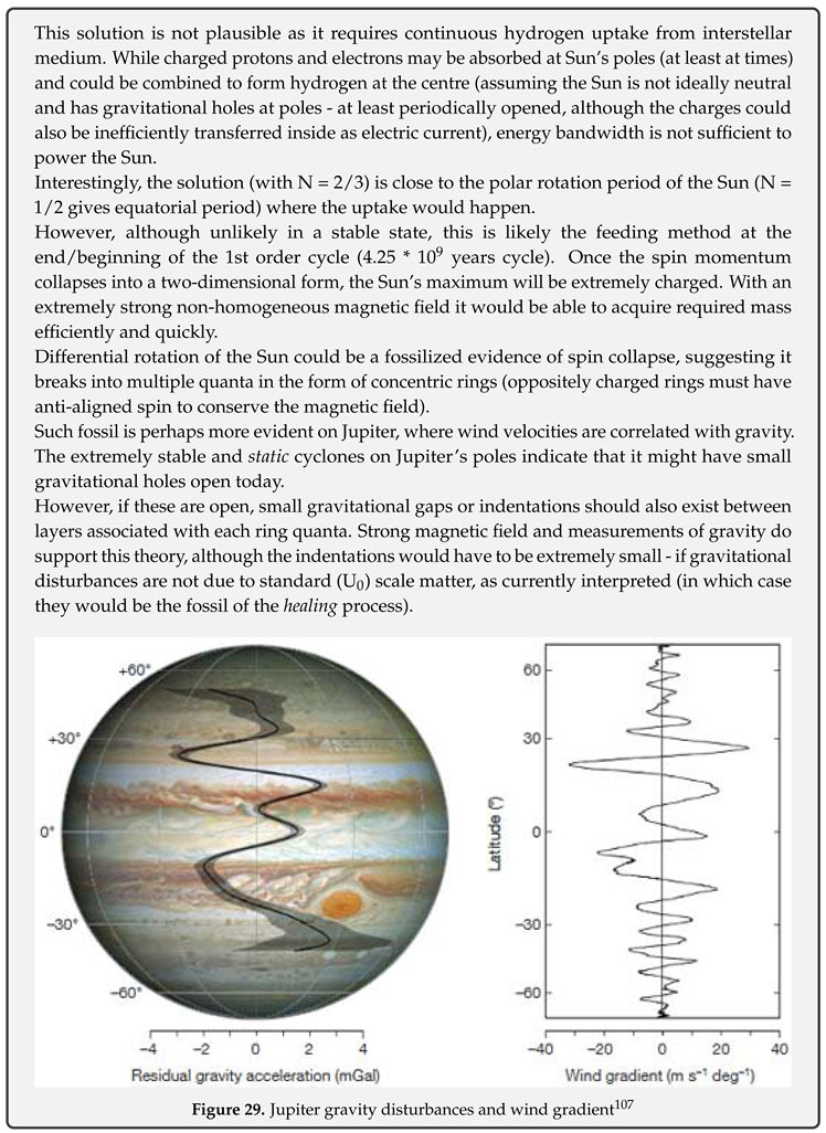
The cells of all living species are regenerating on a periodic basis, for example, 1/3 of hippocampal neurons in humans and mice is exchanged during the lifetime [108], thus, the cellular regeneration in the Sun should not be surprising, whether it is food or constitutional mass.
Capacity for real mass below the Sun’s surface may be full, but all mass orbiting the Sun may be considered as its real mass.
However, it is obviously not fuel mass, rather constitutional or symbiotic mass.
The 3rd order period of the Solar System cycle may be related to this mass through the mass barycentre of the system.
I have previously calculated the neutral gravitational mass equivalent for the surface plasma at the equator which would make its angular velocity Keplerian.
The source for this energy may be the motion of the barycentre.
In any case, if one assumes that conversion between neutral and electro-magnetic component of the general force of the Sun is also periodic and that such energy replaces fusion reactions in equivalent way, the period of recharge is:
and it is in good agreement with the hypothesized 3rd cycle period (a fraction of mass N = 0.6946847 would yield the hypothesized value - 1512000 years).
16.3. As a living organ[ism]
Considering the energy output (metabolic rate) of P = 3.8 * 10 W, the standard relation between metabolic rate and mass[109]:
gives 0.86 for the exponent (M = total mass of the sun = 1988500 * 10 kg). For a mammalian organ this would be between a kidney and a liver[110], suggesting an embryonic stem cell in the process of differentiation.
17. The cycle of life and death
An atom or a planetary system consists of relatively massive matter and relatively empty space of gravitational wells.
The energy of this space is in its vacuum, generally proportional to its spin momentum but also characterized by electric and magnetic permeability of polarized quanta of certain scale.
Gravitational wells (souls) are not intrinsically coupled with matter - otherwise, there would be no death.
All souls thus oscillate between different bodies. This oscillation can be vertical (between different scales) or horizontal (between species of the same element, such as carbon), although even horizontal oscillation includes a temporary scale inflation/deflation between stable states.
Species in horizontal oscillation have comparable lifetimes so gravitational collapse generally indicates a permanent decoupling of particular soul/matter pair (death).
Primary (prevalent) oscillation type depends on pressure/temperature of the environment.
18. Inflation and dark energy
According to CR, observable universe cannot be absolute - if it had a beginning it was a relative beginning and if it was inflated it was inflated from a relative, not absolute, singularity.
The inflation thus did not proceed from a single point, rather inflation of galaxies should be regarded as inflation of spatially separated relative universes even if that separation was relatively small or such that could be considered as quantum-like condensation. Similar is true for planetary systems.
This suggests that development of galaxies was relatively fast and implies there are no large differences between distant and near galaxies when relatively equal energies are involved in their creation (with the assumption of a stable state, dominantly weak and cyclic evolution of components after initial inflation).
If planetary systems are equivalents of standard atoms in a particular state (pressure/temperature), observable universe becomes a gas of extremely low density. Dark energy, if it exists, is thus simply the energy of gas expansion due to scaled pressure/temperature change. Galaxies are then simply large scale quantum vortices.
Black holes and other gravitational wells of U scale can be understood as vacuum quanta, increasing in strength with inflation and causing contraction of constituent matter, with stretched space (at times of inflation of space, not expansion) between them creating (inflating) new gravitational wells (primal stars) between galaxies. This exponential growth of energy is what eventually ends inflation.
The expansion of the observable universe has been questioned before and there are results consistent with a non-expanding, Euclidean universe[114] regarding some phenomena previously considered to favour expanding universe, although none solve all the problems - ie. increasing redshift with distance or time dilation of distant events.
Some recent analyses suggest that the expansion of the observable universe is not accelerating[115] and the redshift previously used as evidence for acceleration should be attributed to local "bulk flow" instead.
If photons have rest mass on some scale, as CR implies, energy will be lost with distance (if not replenished periodically). If the mechanism for energy loss from distant galaxies is not scattering of light through interactions with standard (U scale) matter, the interactions must be involving smaller scales of photon energy components. These are causing changes in values of momentum relatively independent of wavelength, and without affecting direction significantly. Photons, having mass, must have a range - which then explains decreasing brightness with distance.
However, even these interactions cannot explain time dilation, which apparently has been observed in Type Ia supernovae[116].
Signatures of time dilation have also been found in gamma-ray bursts but with lower confidence[117].
In any case, the current accelerating expansion or at least its magnitude should be questionable. Observations also suggest that small scale effects on photon energy are oscillating with distance - consistent with hypothesized oscillation of photon mass, which, periodically results in acceleration rather than deceleration of photons. The oscillation must be correlated with properties of space. If there is no significant loss of energy, energy of the photon may be kept relatively constant through these interactions.
19. Stability of elements
Structure of U elements is entangled with the configuration of U universe. This also makes the stability of isotopes dependent on this configuration.
The stability curve and decay rates of individual isotopes thus change strongly in transition from one cycle state to another, but also oscillate during state lifetime.
Stable isotopes are concentrated along this curve:
where N = N is the number of neutrons, P = P = Z is the number of protons of the isotope and P is the maximum number of protons for a stable element (for the Solar and equivalent systems, P = 82, corresponding to Pb - lead). is the small shift in value of N due to weak evolution through state lifetime ().
where N is the number of neutrons and P the number of protons of the parent system - U.
P is the atomic number (number of protons) of the most stable element - element with maximum number of stable isotopes.
P is the atomic number of the element lying on the N(P,t) curve with P/N ratio equal to P/N.
For the Solar System, in state 6p4n:
Figure 34 shows all stable isotopes of the Solar System (green) and the N(P,t) curve (black).
Figure 34.
Stable isotopes of the Solar System in state 6p4n at t > 1495840 years
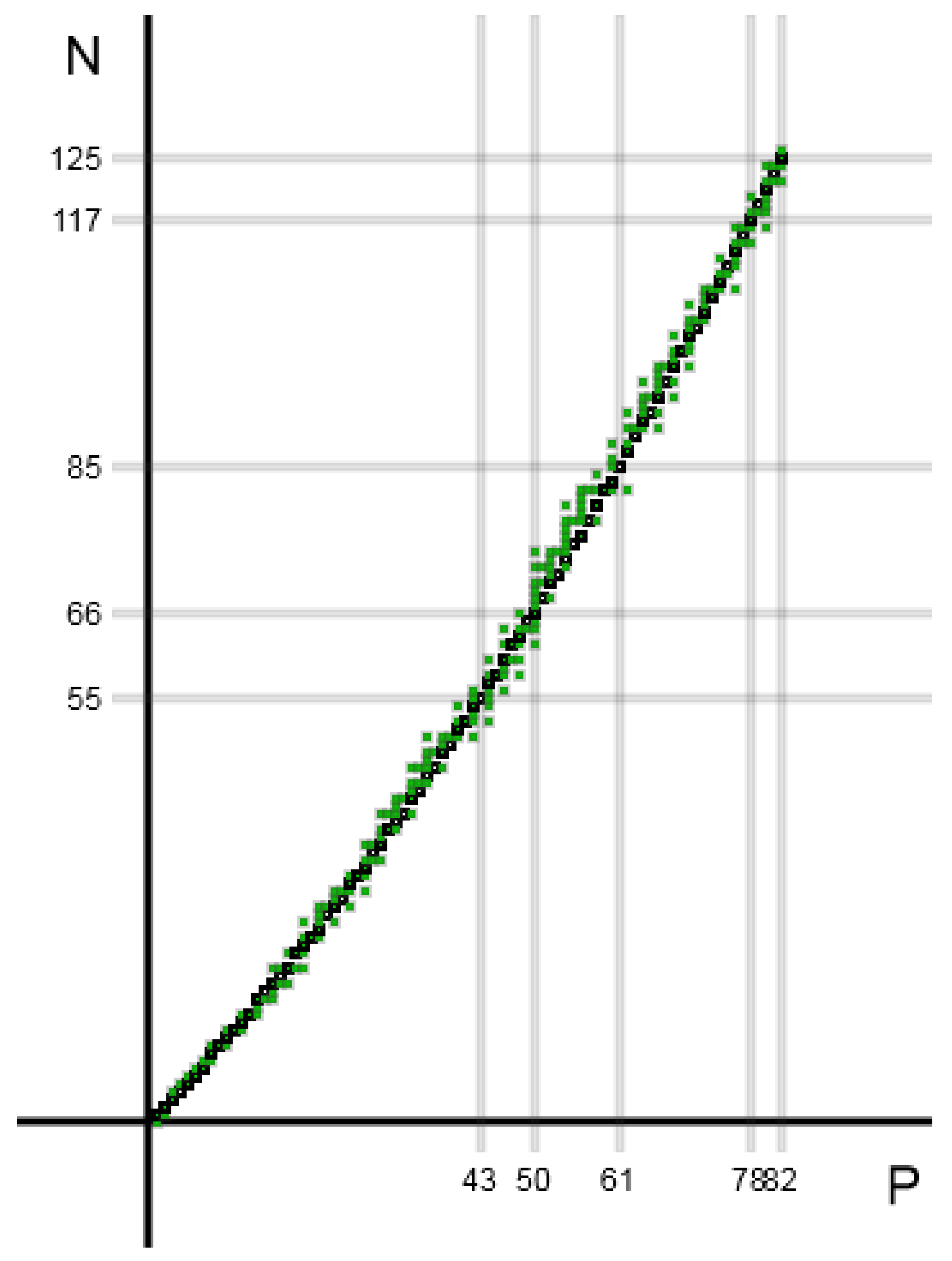
Note the following:
- for t > 1495840 years (t ≈), the isotope lying on the curve with P/N ratio exactly equal to 2/3 is Pt-195 (Platinum, P = 78). The placement of other Platinum isotopes is symmetric relative to the curve,
- for = 0 (t = 3/5 ), the P isotope is Pb-205 (Lead, P = 82). At t = 3/5 this was a stable isotope. 1/3 of other stable isotopes are above the curve, 2/3 below,
- for t = 4/5 the P isotope is Hg-200 (Mercury, P = 80). 1/3 of other stable isotopes are above the curve, 2/3 below,
- the ratio of horizontal to vertical distance between Lead-205 and Platinum-195 is (82 - 78) / (123 - 117) = 4/6 = 2/3,
- the ratio of horizontal to vertical distance between Lead-205 and Hg-200 is (80 - 78) / (120 - 117) = 2/3,
- at t ≈, Tin (Sn, P = 50) has the highest number of stable isotopes (10). Tin isotope lying on the curve is Sn-116 (50 protons, 66 neutrons). 2/3 of other stable Tin isotopes is above the curve, 1/3 is below,
- at t ≈, the only elements without stable isotopes are Tc (Technetium, P = 43) and Pm (Promethium, P = 61). The isotopes lying on the curve are Tc-98 and Pm-146. Vertical distance from Sn-116 to Tc-98 is equal to horizontal distance from Sn-116 to Pm-146.
20. Electric gravity
According to CR, electric force is a polarized component of the general force.
Inside the atom, force field between negative and positive charges is neutralized and electro-magnetic potential may be exchanged with gravitational potential.
Thus, a Hill sphere radius (r) of an atom should be correlated with its charge radius.
This gives, for Carbon-12 atom with nucleus mass m = 1.992646883 * 10 kg inside the gravity field of Earth at R = 6371 km (surface):
This is in agreement with experimentally obtained radius of 70 pm (±5 pm). Calculation for other elements of the periodic table yields similar results.
Note that Hill radius is different for different isotopes of the same element while experimentally obtained atomic radii are charge radii and thus independent of the number of neutrons (radius represents the orbit of the outermost electron). In example, for Carbon-14 the obtained value is 69.5 * 10 m, and even closer to 70 pm if one calculates using equatorial radius of Earth instead of mean volumetric (a possible indicator that the Solar System soul was a part of a (C-N-O) cycle in previous incarnation).
Figure 35 shows experimentally obtained radius (green) and calculated Hill sphere at R = 6371 km (black) for all stable isotopes. Evidently, radii are not only correlated but values of covalent radii oscillate around the Hill radii, confirming the entanglement of U and U.
Figure 35.
Calculated Hill sphere and measured radius for stable isotopes: a) data from 2008. b) data from 1964.
Figure 35.
Calculated Hill sphere and measured radius for stable isotopes: a) data from 2008. b) data from 1964.
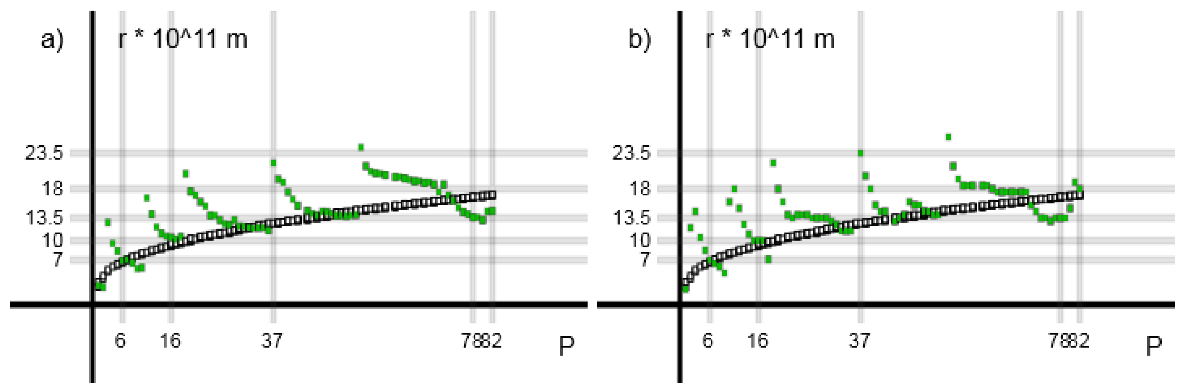
Comparing data from 1964.[118] and 2008.[119] shows a compression of radii and convergence to Hill radii - such changes are expected in CR (no constants) and these should be accelerating as the Solar System approaches the end of the current state (6p4n).
In the intermediate state (5p5n) charges may be completely neutralized, and the radii of all elements may converge to Hill radius.
Figure 36 shows the experimentally obtained radius (green squares) and calculated Hill sphere at R = 6371 km (black squares) for isotopes with neutron number adjusted to match the charge radius.
Figure 36.
Calculated Hill sphere (adjusted) and measured radius for stable isotopes: a) data from 2008. b) data from 1964.
Figure 36.
Calculated Hill sphere (adjusted) and measured radius for stable isotopes: a) data from 2008. b) data from 1964.

In calculations above, atomic mass has been quantized by u = 1.66053907 * 10 kg (atomic mass constant) with integer number of protons P and neutrons N [m = (P + N) * u] so Hill radii are quantized too. The overlap of Hill radii with charge radii in Figure 36 shows that charge radius is quantized too (there is a number of neutrons N for which the Hill radius will match the charge radius).
Figure 37 shows the number of neutrons N used with each element to obtain Hill radius equal to charge radius.
Figure 37.
Isotopes used in Figure 36 calculation: a) data from 2008. b) data from 1964.
Figure 37.
Isotopes used in Figure 36 calculation: a) data from 2008. b) data from 1964.
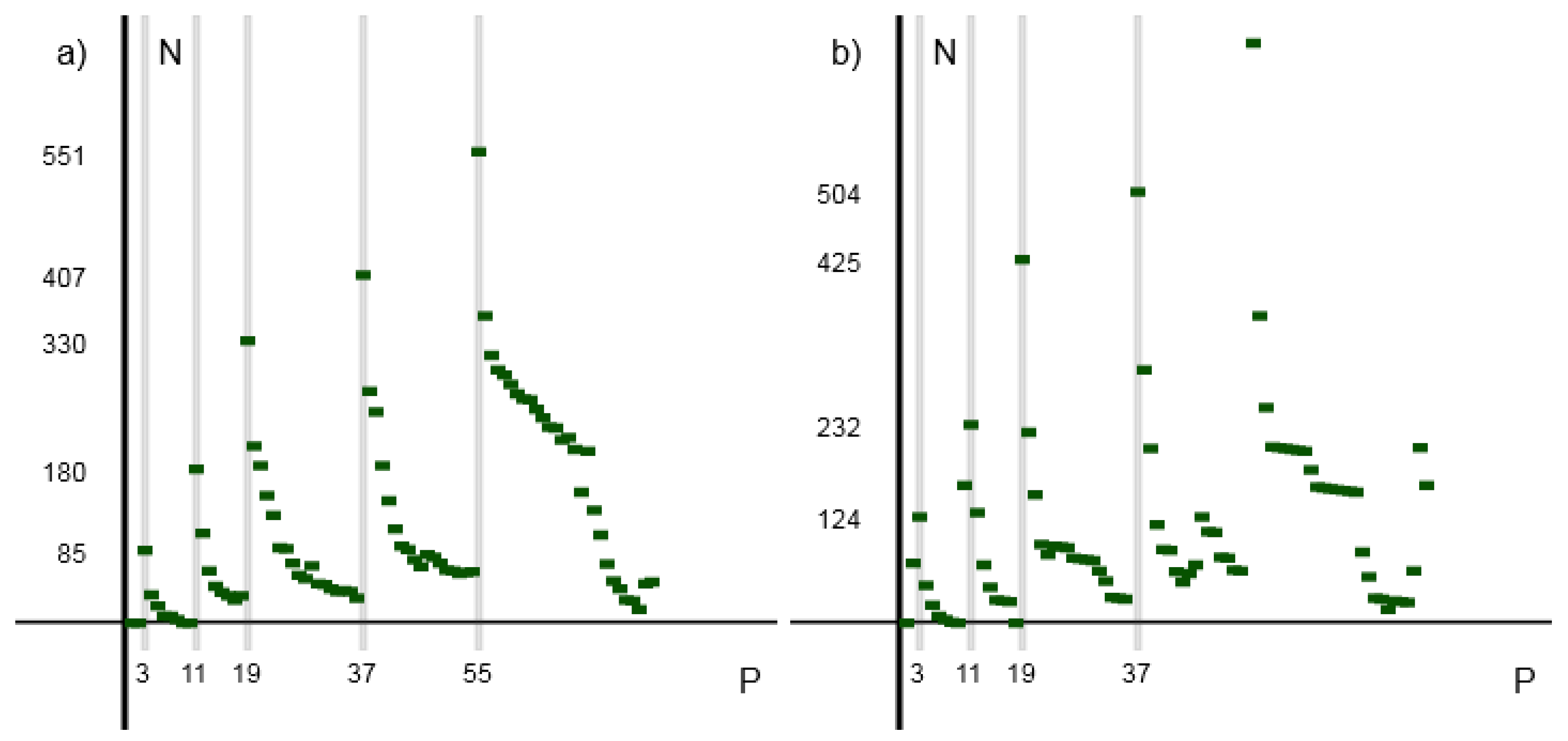
From above figures it is obvious that elements (atoms) can be grouped into shells the same way as electrons are grouped within atoms.
Grouping is shown in Table 40. There are two possibilities - either the shells L, M and N are doubled or the grouping is reflected after the N shell, so shells O, P and Q contain the same number of elements such as shells N, M and L, respectively. Note that in case of alternative (Og) grouping, no elements beyond Og are theoretically possible - otherwise another shell would be present between He and Li.
Gravitational constant G is not dimensionless and therefore not invariant to vertical scale transformation.
On the standard atom scale U, gravitational constant for a completely neutralized general force can be derived from previously obtained orbital momentum of the Carbon-10 outermost electron:
v = v = 5.585837356 * 10 m/s
r = r = 70 * 10 m
where m, v, r are components of the outermost electron orbital momentum (mass, velocity, radius).
If one now, equalizes electric with gravitational force (for photon/graviton m > 0 - Yukawa, Proca[120]):
discarding / r factors due to being practically equal and equal to 0 on both sides (expecting large r):
ℏ = reduced Planck’s constant = 1.054573 * 10 Js
c = 2.99792458 * 10 m/s
k = Coulomb constant = 8.9875517873681764 * 10 Nm/C
Q = electron charge = 1.60217733 * 10 C
M = photon mass
M = U graviton mass
Using previously obtained photon mass M = 2 * 9.10938356 * 10 kg and carbon graviton mass M = 2 * 1.663337576 * 10 kg, this gives:
as the distance in space when two forces become equal.
The fact that obtained distance is equal to the radius of observable universe is not a coincidence.
For an inflation at the speed of light, for standard particles, distance in space is distance in time so this may be interpreted as the time when both forces (carrier masses) were equal, after which point one particle started losing mass while the other was gaining mass.
This is expected with the exchange of one potential for the other.
In the past the observable universe likely did expand, but geometry deformation was localized (quantized, gravitational wells being the quanta of vacuum) and expansion may have lasted only up to the point of CMB emission (at this point the speed of light also became equal to c). The redshifts thus may be caused by lower scale (U) particles in intergalactic medium absorbing photon energies.
Taking into account the scaled density of the observable universe (gas), evidently this is a discontinuity, and possibly a gravitational maximum between layers of, relatively, dense matter.
If its angular velocity is equal to c, this is a black hole maximum (escape velocity = c).
Thus, light coming from large distances might be the light reflected off of the firewall, providing a window to the past of inner content. This explains correlation of apparently spatially separated phenomena (galaxies) - these may not be images of different phenomena separated in space, but one separated in time.
Note that, if one fixes the gravitational constant G to
one obtains this:
where is the vacuum permeability (magnetic) constant and K = 1 C/m.
One can now obtain k and Q for the U scale (Solar System):
Using G = 6.674 * 10 m/kgs and previously obtained c = 2.930445979 * 10 m/s:
Ranges on U scale:
Using m = 1.02413 * 10 kg and previously obtained M = 1.663337576 * 10 kg, M = 9.10938356 * 10 kg, the distance where two forces become equal, r = 1.0059686 * 10 m ≈ 1 * 10 m.
Note that, if one fixes m to
one obtains this:
where M = 1.6726218977 * 10 kg is the mass of a standard proton.
Range of U electric force:
Range of U gravitational force:
Here, unit m (meter) is unscaled, for a properly scaled metric the ranges are equal to ranges on U scale.
21. Relation of G variation to Sun’s discontinuities
Equalizing the strength of electric and gravitational force between two free particles (positron and electron), disregarding small mass of carrier particles:
yields the following value for the gravitational constant G:
k = 8.9875517873681764 * 10 Nm/C
Q = 1.60217733 * 10 C
M = 9.10938356 * 10 kg
In CR, gravitational constant G changes with scale. But it is also modified with neutralization of EM force, when k decreases, while G increases.
This enables the gravitational force to be, at least in some cases, a prevailing force in the atom, rather than EM force.
I have previously calculated G relative to a C atom nucleus mass obtained through current Sun mass, the constant G using rest mass of C nucleus is:
v = 5.5550351679 * 10 m/s
r = 70 * 10 m
M = 1.663337576 * 10 kg
where m, v and r are components of the orbital angular momentum of the outermost electron.
Calculated G (G) is now only 5 orders of magnitude smaller than G required for gravity to be equal in strength to EM force between an electron and a positron.
But instead of G increasing, one might assume that k decreases by 5 orders of magnitude, or more precisely by this amount:
Thus, the increase of G (G) of Earth’s inner core maximum, after extraction, neutralization and collapse to current radii, is equal to k.
I have previously calculated that this G has increased to 5.731534632 * 10 m/kgs, which is, relative to surface G (6.674 * 10 m/kgs), an increase of:
which is also the ratio between imaginary mass M (5.97 * 10 kg) and real mass m (6.95 * 10 kg) of Earth from some reference frames.
But what was the initial G of Earth’s inner core?
According to above hypothesis, it should have been:
If Earth’s core has been extracted from the Sun, as hypothesized, one can get its original radius using this constant:
M = img mass of the Sun = 1.988500 * 10 kg
g = gravity of the maximum = 274 m/s
This agrees very well with the hypothesis of entanglement of discontinuities with inner planetary orbitals:
R = Sun radius = 695700 km
r = Earth orbital = 149.6 * 10 km
r = Mars orbital = 227.92 * 10 km
The discontinuity (r/R = 0.63) is evident through the profile of rotational velocities of the Sun:
Above this discontinuity is the tachocline (transition region between the radiative and convective layer of the Sun), a major source of the Sun’s magnetic dipole, analogous to the region of charge above Earth’s inner core.
The hypothesis of neurogenesis, assuming pending neurogenesis on Earth and completed neurogenesis on Mars and other terrestrial planets, explains why Earth is the only one with an active surface magnetic dipole. The connection of tachocline with 0.63R discontinuity would suggest:
- its position is not permanent and it moves between discontinuities, corresponding to the planet with ongoing neurogenesis,
- possible multiple active discontinuities and associated tachoclines in the past, initially at maximum, or
- current position is the place of birth of all planetary embryos (cores).
The 2nd hypothesis here is most plausible - the tachocline is active as long as the magnetic dipole of the corresponding planet is active (the two phenomena are synchronized).
However, if the tachocline is localized to 0.71R [122] and distance between the tachocline and the discontinuity is scaled from Earth (distance between the charge radius and gravitational maximum), the associated discontinuity is at:
which would be a discontinuity associated with Venus.
In that case the tachocline is the location of a charge radius associated with a 0.5R gravitational maximum and, assuming equal g-factor, such charge radius should also be located at:
In this case though, the g-factor of a neutron might be more appropriate, yielding r = 1.111507303 * 10 km (and a mirror at 444533.257 km = 0.639R).
Note that the 0.71R tachocline is 3/4 of 0.94R, which according to Figure 38 seems to be another discontinuity or a fossilized initial Sun radius.
Figure 38.
Sun rotation rates
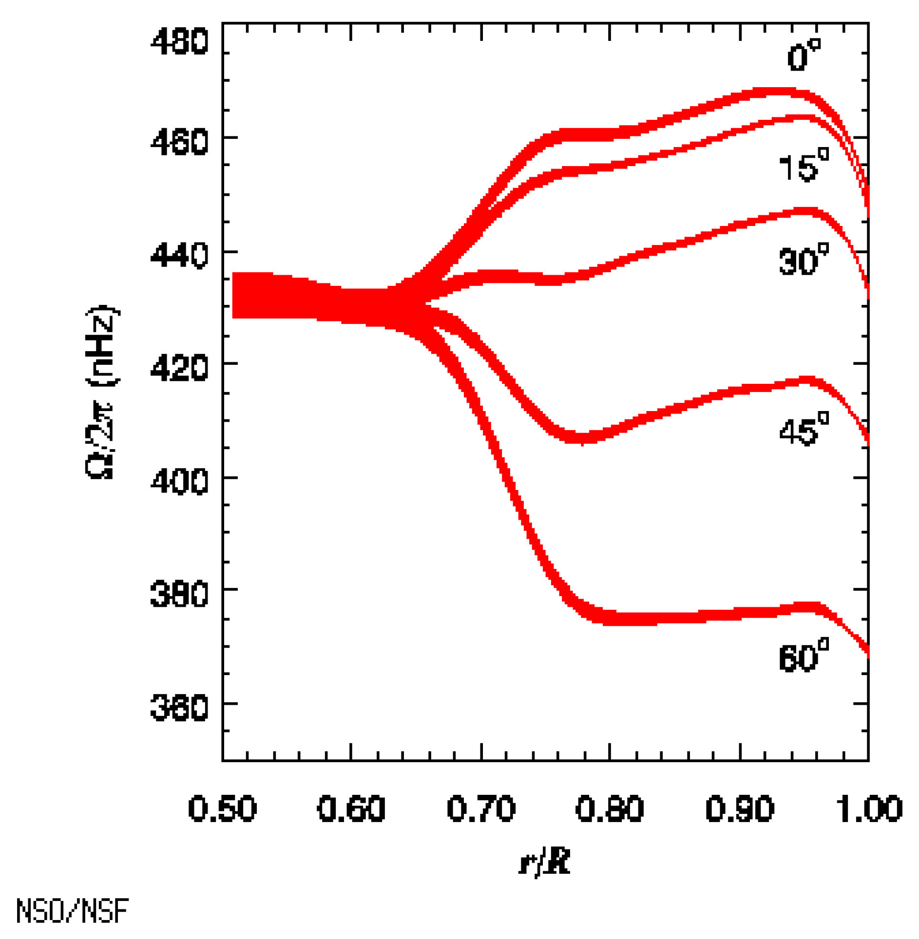
Such fossil is also visible at 0.75R, which should be a discontinuity in 4p6n state.
The 0.63R (2/3 of 0.94R) is also a fossil, as the current location associated with Earth is 0.66R.
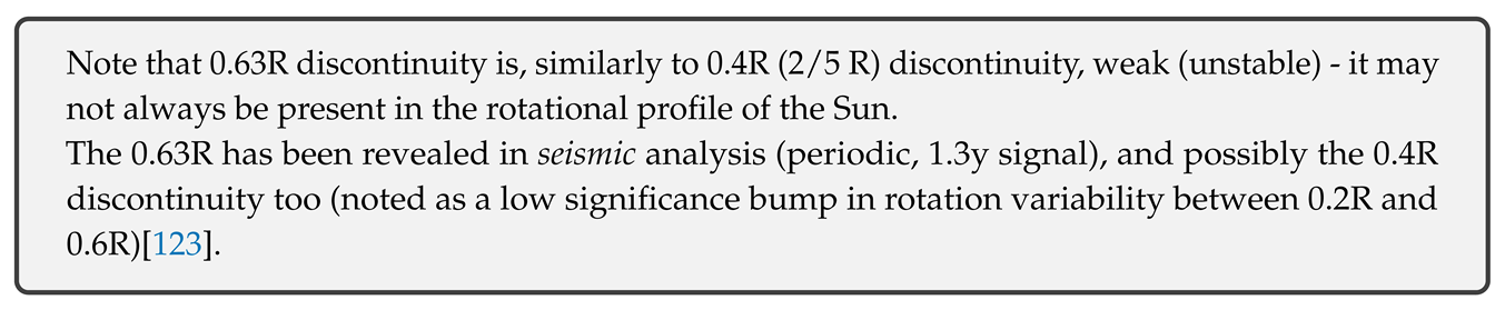
Sun’s GM product has increased 0.06% due to relativistic energy relative to CMB, so initial radius at 0.94R implies that surface radius changes proportionally:
for previously obtained c = 2.93 * 10 m/s and v = v + v = 996 km/s, gives R = 654271.142 km = 0.94 R.
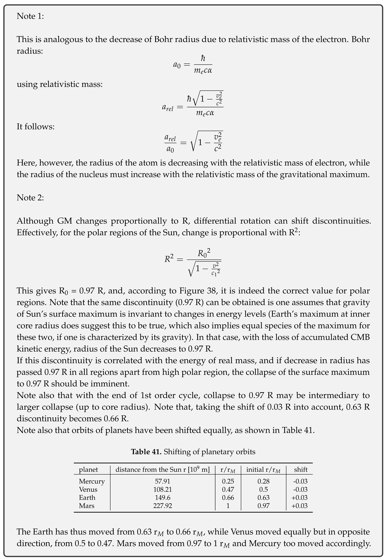
22. Gyro-magnetic ratio and its correlation with Earth/Moon
The gyro-magnetic ratio of a particle is the ratio of its magnetic moment to its angular momentum:
With the assumption that mass and charge have equal momentum:
where q, m are charge and mass of the particle, respectively.
Measurements show that this is not valid for quantum particles such as electron. Thus, a dimensionless factor g (g-factor) was introduced:
The factor has been attributed to quantum effects which do not exist in classical (intuitive) reality - point particles with intrinsic magnetic moment (no rotation).
The notion of point particles having any properties is in itself problematic, let alone existence of different point particles with different properties. However, if such particles could exist, due to scale invariance, they would have to exist on bigger scales too. No such thing has ever been observed in reality - all magnetic fields are produced by moving charges of objects having a real radius.
Thus, intrinsic magnetic momentum is not intuitive, but intrinsic rotation of charge (producing the momentum) at finite radius greater than 0 is.
In CR there is also no intrinsic coupling of matter and gravity, and since charge field is a polarized gravitational field, the g-factor can be explained simply by a difference in distribution (or angular momenta) of gravitational mass and charge mass within the particle, preserving the intuitive concepts of reality.
Complete relativity not only allows speeds faster than light (photon mass is scale dependent) but implies such speeds must exist at some scale, thus the required superluminal rotation of charge (implied at certain radii) in particles such as an electron is not an issue either.
The absolute (invariant) speed limit is not a dimensionless constant and thus is counter-intuitive in scale invariant reality (relativity), but, in this case, the required speed would be valid even in the context of General Relativity (charge is at rest relative to rotating space) if it would incorporate scale invariant curvature of space.
Magnetic moment µ and angular momentum L:
where v, r are the charge orbital velocity and radius, respectively, and v, r are the mass orbital velocity and radius, respectively.
The factor g is thus:
Being dimensionless, it should be scale invariant relative to particle flavor.
This means that the value of g for electron and positron is equal to g of Earth, as Earth is a large scale Dirac fermion equivalent (obviously not a point particle unless taken relatively), albeit in an environment where its fermionic nature is effectively annihilated.
Just like the electron, Earth consists of intrinsic charge and mass and accumulated mass due to neutralization.
The intrinsic energy is concentrated within the inner and outer core.
Assuming charge radius is in the outer core where gravity equals g = 137 m/s and gravitational mass radius is the inner core gravitational maximum g (274 m/s), with equal rotation period (and angle between v and r vectors):
Note that it was assumed that mass is not a solid body with radius r but, like the charge, a particle or a stream of particles forming a ring at r.
This is a valid assumption since this mass is not real mass, but vacuum energy (imaginary mass) which, in case of charged naked maxima, forms a ring rather than sphere surface.
Figure 39.
Mass and charge radii of charged bodies
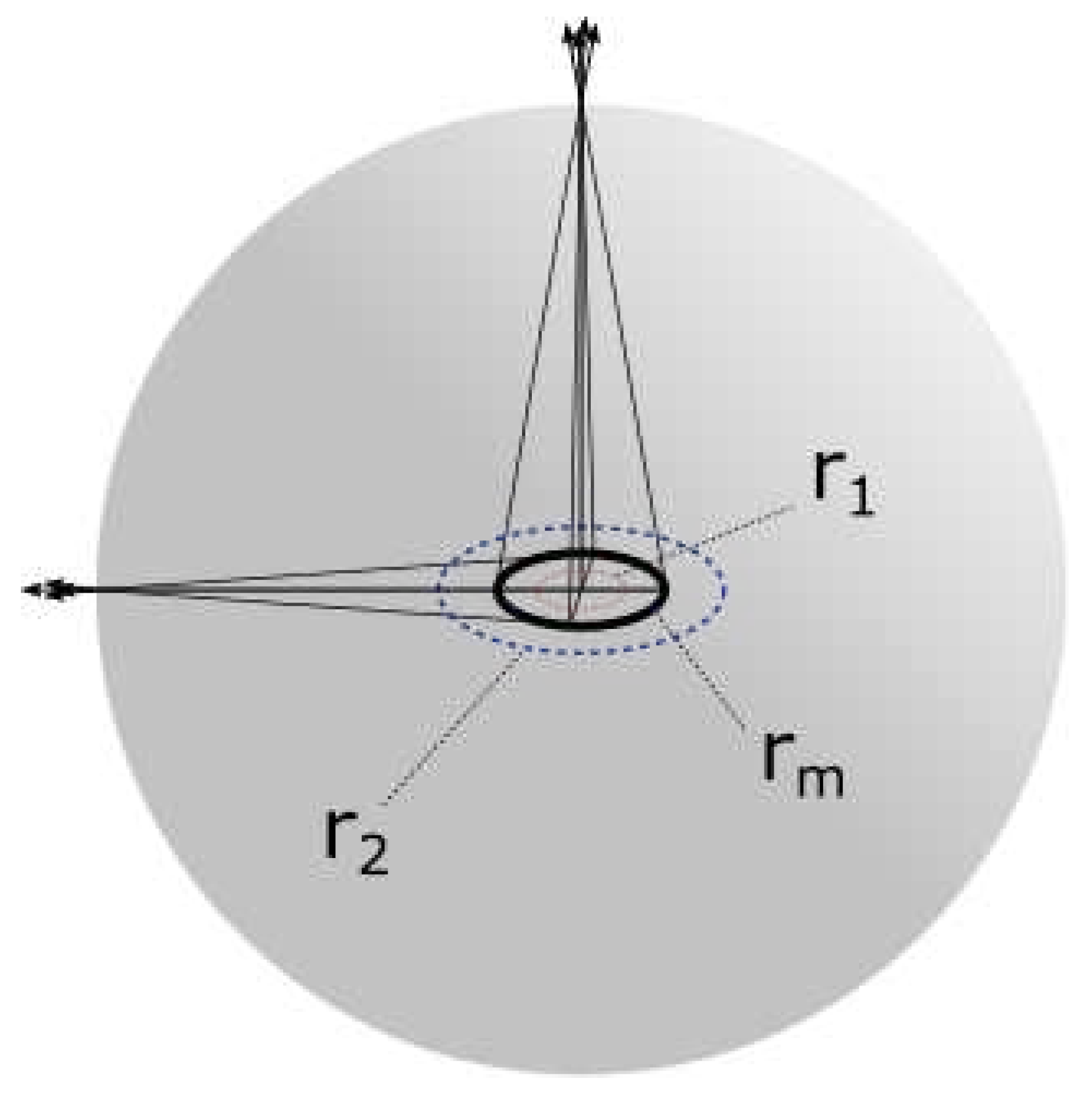
Since gravitational potential is not isotropic, gravitational acceleration at any point is a vector sum of accelerations induced by vacuum quanta forming the ring:
In case of equatorial and polar gravity vector components parallel to surface cancel out. Equatorial gravity is thus:
where R is the equatorial radius.
Polar gravity:
where R is the polar radius.
Deriving GM product with equatorial gravity fixed to 9.798 m/s and calculating polar gravity, for n >= 5, gives 9.34 m/s.
This is smaller than measured, so the Earth must be a composite of 2 positrons (or positron equivalents), as hypothesized.
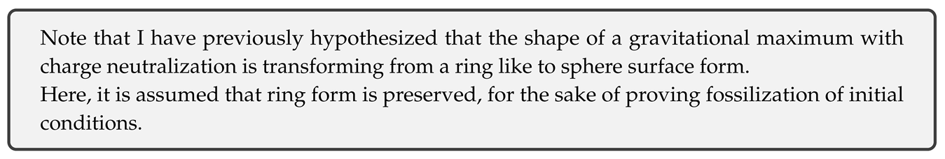
With 2 particles in the same state, energy splits into two levels:
Figure 39.
Mass and charge radii of two charged bodies sharing a single state
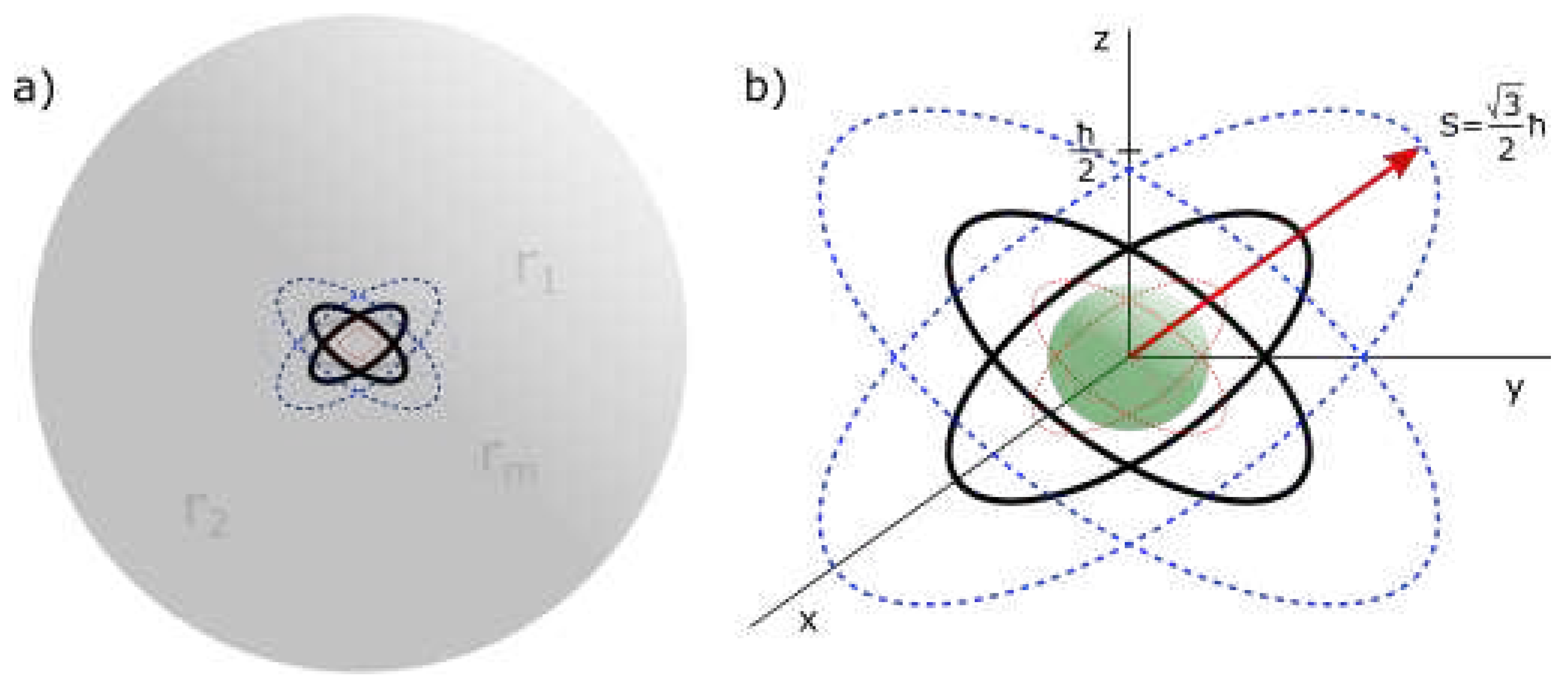
In such state, two charges are deflected from the equator by this angle:
Charges are thus separated by 2*35.2643896827547 = 70.5287793655094 (two magnetic north poles on Jupiter seem to be separated by this angle, confirming its 2e configuration).
Confirmation of this configuration of Earth comes from the state of the Moon (Luna) and non-alignment of Earth’s north and south magnetic poles.
Initial total obliquity of Luna relative to Earth’s equator is 23.44 + 5.14 + 6.68 = 35.26, equal to .
The Moon orbits one of Earth’s positrons and its obliquity shows that it is built around one of the collapsed gravitational maxima of this positron.
One can thus expect this positron to have smaller contribution to gravity and charge of Earth. Further splitting of energy levels due to carbon configuration can also be expected, so number of quanta should be 6 in one positron and 5 in the other (1 is in the Moon).
It appears that, in the collapse, 6.68 of Luna’s obliquity to Earth’s equator has been exchanged for obliquity to Luna’s own orbital plane, this can be due to influence from another body, but, since the loss of one quantum causes asymmetry in charge distribution it is more likely that this is the exact amount by which the inner positron decreased its angle to Earth’s equator.
Thus, one can expect the orbital plane of this positron to be aligned with the orbital plane of the Moon.
This can then be interpreted as redistribution of charges on the plane, rather than loss. The Moon is thus the reason why Earth still has a dipole magnetic field - with symmetric anti-aligned positron spins the magnetic dipole would be cancelled.
Bigger moons and/or an increased number of moons (with distinct gravitational wells) of outer planets with stronger magnetic fields are thus no surprise and indicate core asymmetry if the spins are anti-aligned (note that a symmetric core does not indicate a planet has no moons, rather that it has the same number of them on each orbital plane).
But rather than the extraction of the Moon core from Earth, in the current, progressive evolution a reverse scenario is more plausible.
Even if the first positron was not fragmented from the beginning, massive extinctions that happened on Earth suggest the second one arrived quantum by quantum on a periodic basis.
There were 5 massive extinctions and there are 5 quanta of the positron in the core, 1 in the Moon.
As the mammal brain has 6 layers, with 6th layer sparsely populated, the theory of neurogenesis is strongly aligned with this hypothesis. Note that the sparse neuron cell population of the 6th layer now indicates an underdeveloped layer - the direct cause for this is the distance of the Moon.
23. Conclusion
The aim of this paper was to provide good evidence for Complete Relativity, which, I am convinced, it has succeeded in. Indeed, the analysis reveals plenty of correlation and equivalence between small scale and large scale systems that cannot be easily dismissed as coincidence.
Strong correlation of Earth’s mantle layers with major extinction events is a strong evidence for planetary neurogenesis. The existence of a discontinuity at 100 km depth even suggests that the formation of a mantle discontinuity precedes surface extinction. This shows that surface extinctions are programmed events, which, however, is not surprising for a neurogenesis of an evolving life-form (one would expect for a brain layer to be at least roughly formed before neurons migrate to that layer).
Some questions remain, however, and there are predictions and hypotheses that require additional experiments and observation to be confirmed or refuted.
References
- Complete Relativity: Nature of observables (2022), Amenoum. https://amenoum.org/complete_relativity.html.
- NASA Planetary Fact Sheet. https://nssdc.gsfc.nasa.gov/planetary/factsheet/.
- Images of planets (2013), OpenClipart-Vectors. https://pixabay.com/users/openclipart-vectors-30363/.
- Six transiting planets and a chain of Laplace resonances in TOI-178 (2020), A. Leleu et al. [CrossRef]
- CODATA recommended values (2018), NIST. https://physics.nist.gov/cuu/Constants/bibliography.html.
- Complete Relativity: Nature of observables (2022), Amenoum. https://amenoum.org/complete_relativity.html#tag_determination_of_c_n.
- Putovanje kroz vrijeme (2021), Amenoum. https://amenoum.org/log/31_putovanje_kroz_vrijeme.html.
- Rest mass of photon on the surface of matter (2020), M. Goray et al. [CrossRef]
- An Electroweak model with electrons of opposite helicities carrying the same quantum numbers (1981), W. B. Yeung.
- S62 on a 9.9 yr Orbit around SgrA* (2020), F. Peißker et al. [CrossRef]
- S62 and S4711: Indications of a Population of Faint Fast-moving Stars inside the S2 Orbit—S4711 on a 7.6 yr Orbit around Sgr A* (2020), F. Peißker et al. [CrossRef]
- On the Formation of Compact Stellar Disks around Sagittarius A* (2008), M. Wardle et al. [CrossRef]
- Asymptotic g modes: Evidence for a rapid rotation of the solar core (2017), Fossat et al. [CrossRef]
- Micrometeoroid infall onto Saturn’s rings constrains their age to no more than a few hundred million years (2023), S. Kempf et al, Science Advances, 9(19). [CrossRef]
- Measurement and implications of Saturn’s gravity field and ring mass (2019), L. Iess et al, Science, 364(6445). [CrossRef]
- Long-term patterns of body mass and stature evolution within the hominin lineage (2017), M. Will et al. [CrossRef]
- Cosmogenic radionuclides reveal an extreme solar particle storm near a solar minimum 9125 years BP (2022), C. I. Paleari et al. [CrossRef]
- On the Origins of Magnetic Excursions in the Great Lakes (1981), W. F. Kean. [CrossRef]
- The Norwegian-Greenland Sea, the Laschamps, and the Mono Lake Excursions Recorded in a Black Sea Sedimentary Sequence Spanning From 68.9 to 14.5 ka (2020), J. Liu et al. [CrossRef]
- The Lake Mungo geomagnetic excursion (1976), M. F. Barbetti and M. W. McElhinny. [CrossRef]
- The 26.5 ka Oruanui eruption New Zealand: An introduction and overview (2001), C. J. N. Wilson. [CrossRef]
- Robust Characteristics of the Laschamp and Mono Lake Geomagnetic Excursions: Results From Global Field Models (2019), M. Korte et al. [CrossRef]
- Evidence for two intervals of enhanced 10Be deposition in Antarctic ice during the last glacial period (1987), G. M. Raisbeck et al. [CrossRef]
- Late Pleistocene geomagnetic excursion in Icelandic lavas: confirmation of the Laschamp excursion (1990), S. Levi et al. [CrossRef]
- The Toba supervolcano eruption caused severe tropical stratospheric ozone depletion (2021), S. Osipov et al. [CrossRef]
- The Gothenburg Magnetic Excursion (1977), N. Mörner. [CrossRef]
- Evidence for an extraterrestrial impact 12900 years ago that contributed to the megafaunal extinctions and the Younger Dryas cooling (2007), R. B. Firestone et al. [CrossRef]
- The 13 million year Cenozoic pulse of the Earth (2015), J. Chen. [CrossRef]
- When and Why Did Human Brains Decrease in Size? A New Change-Point Analysis and Insights From Brain Evolution in Ants (2021), J. M. DeSilva et al. [CrossRef]
- On the 1470-year pacing of Dansgaard-Oeschger warm events (2002), M. Schulz. [CrossRef]
- The Relationship of Sunspot Cycles to Gravitational Stresses on the Sun: Results of a Proof-of-Concept Simulation (2011), D. Jassby. [CrossRef]
- Internal rotation of Sun (2010), SOHO. https://ase.tufts.edu/cosmos/view_picture.asp?id=1368. 1368.
- Velocity Curves for Spiral Galaxies (2015), C. R. Nave. http://hyperphysics.phy-astr.gsu.edu/hbase/Astro/velcurv.html.
- Discovery of variation in Solar coronal rotation with altitude (2001), H. O. Vats et al.
- A Quantum-Like Description of the Planetary Systems (2007), F. Scardigli. [CrossRef]
- Self-Organizing Systems in Planetary Physics: Harmonic Resonances of Planet and Moon Orbits (2018), M. J. Aschwanden. [CrossRef]
- The deep Earth may not be cooling down (2016), D. Andrault et al. [CrossRef]
- Complete Relativity: Nature of observables (2022), Amenoum. https://amenoum.org/complete_relativity.html#tag_total_mass.
- Eccentricity of the geomagnetic dipole caused by lopsided inner core growth (2012), P. Olson et al. [CrossRef]
- Search for new phenomena in dijet events with the ATLAS detector at s = 13 TeV (2019), D. Zhang. https://cds.cern.ch/record/2683921/files/ATL-PHYS-SLIDE-2019-426.pdf.
- Signals of a 2 TeV W’ boson and a heavier Z’ boson (2016), B. A. Dobrescu et al. [CrossRef]
- Complete Relativity: Nature of observables (2022), Amenoum. https://amenoum.org/complete_relativity.html#ref12.
- NIST Atomic Spectra Database ver. 5.9 (2021), A. Kramida et al. [CrossRef]
- Assessments of the energy, mass and size of the Chicxulub Impactor (2014), H. J. Durand-Manterola and G. Cordero-Tercero. [CrossRef]
- Distributions and moments of asteroid and comet impact speeds upon the Earth and Mars (1998), D. Steel. [CrossRef]
- Solar Wind Implantation Into the Lunar Regolith: Monte Carlo Simulations of H Retention in a Surface With Defects and the H2 Exosphere (2018), O. J. Tucker et al. [CrossRef]
- Solar Storms Could ’Sandblast’ the Moon (2011), NASA. https://www.nasa.gov/topics/solarsystem/features/dream-cme.html.
- Multiple Impacts at the KT Boundary and the Death of the Dinosaurs (1997), S. Chatterjee.
- 99942 Apophis Earth Impact Risk Summary (2013), NASA. https://web.archive.org/web/20130512035601/http://neo.jpl.nasa.gov/risk/a99942.html.
- Measurements of Newton’s gravitational constant and the length of day (2015), J. D. Anderson et al. [CrossRef]
- Horizons On-Line Ephemeris System (2020), NASA Solar System Dynamics Group. http://ssd.jpl.nasa.gov/.
- Equatorial anisotropy in the inner part of Earth’s inner core from autocorrelation of earthquake coda (2015), T. Wang et al. [CrossRef]
- A complex dynamo inferred from the hemispheric dichotomy of Jupiter’s magnetic field (2018), K. M. Moore et al. [CrossRef]
- Uranus fact sheet (2019), NASA/GSFC. https://nssdc.gsfc.nasa.gov/planetary/factsheet/uranusfact.html.
- Neptune fact sheet (2019), NASA/GSFC. https://nssdc.gsfc.nasa.gov/planetary/factsheet/neptunefact.html.
- Up-to-fivefold reverberating waves through the Earth’s center and distinctly anisotropic innermost inner core (2023), T. Pham and H. Tkalčić. [CrossRef]
- Antipodal hotspots and bipolar catastrophes: Were oceanic large-body impacts the cause? (2005), J. T. Hagstrum, Earth and Planetary Science Letters 236(1-2), 13-27. [CrossRef]
- Broad plumes rooted at the base of the Earth’s mantle beneath major hotspots (2015), S. French and B. Romanowicz, Nature 525, 95–99. [CrossRef]
- On the resolution of seismic tomography models and the connection to geodynamic modelling (2019), EGU. https://blogs.egu.eu/divisions/gd/2019/06/05/on-the-resolution-of-seismic-tomography-models-andthe-connection-to-geodynamic-modelling-is-blue-red-the-new-cold-hot-how-many-pixels-in-an-earth/.
- 10Be: Half-life and AMS-standards (1987), H. J. Hofmann et al. [CrossRef]
- A new value for the half-life of 10Be by Heavy-Ion Elastic Recoil Detection and liquid scintillation counting (2010), G. Korschinek et al. [CrossRef]
- Rest Heart Rate and Life Expectancy (1997), H. J. Levine. [CrossRef]
- The species of homo (2022), Amenoum. https://amenoum.org/log/25_species_of_homo.html.
- Athropogenic carbon and ocean pH, Nature 425, 365 (2003), K. Caldeira et al.
- Ocean acidification and the Permo-Triassic mass extinction (2015), M. O. Clarkson et al. [CrossRef]
- Essentials of geology, 4th edition, 256 (2013), S. Marshak.
- Characteristic disruptions of an excitable carbon cycle (2019), D. H. Rothman. [CrossRef]
- Thresholds of catastrophe in the Earth system (2017), D. H. Rothman. [CrossRef]
- Do Red and Green Make Brown?: Perspectives on Plastid Acquisitions within Chromalveolates (2011), R. G. Dorrell et al. [CrossRef]
- Future climate forcing potentially without precedent in the last 420 million years (2017), G. L. Foster et al. [CrossRef]
- Periodicity of extinctions in the geologic past (1983), D. M. Raup et al. [CrossRef]
- Periodic impact cratering and extinction events over the last 260 million years (2015), M. R. Rampino et al. [CrossRef]
- No Evidence for a Large Atmospheric CO2 Spike Across the Cretaceous-Paleogene Boundary (2019), J. N. Milligan et al. [CrossRef]
- Chart: Atmospheric CO2 Levels Are Rising (2018), Inside Climate News. https://insideclimatenews.org/infographics/chart-atmospheric-co2-levels-have-been-rising/.
- Understanding synchronicity (2020), Amenoum. https://amenoum.org/log/19_understanding_synchronicity.html.
- Never at rest: A biography of Isaac Newton (1983), R. S. Westfall, 816-817.
- Amenoum (2020), Amenoum https://amenoum.org/authors/Amenoum.html.
- 10Be β- Decay Evaluated Data (2019), TUNL Nuclear Data Evaluation Project. https://nucldata.tunl.duke.edu/nucldata/GroundStatedecays/10Be.shtml.
- Evidence of correlations between nuclear decay rates and Earth–Sun distance (2009), J. H. Jenkins et al. [CrossRef]
- Where is the Earth’s Radiogenic Helium? (1957), L. G. Carpenter et al. https://www.nature.com/articles/179213a0.
- Paleosol barometer indicates extreme fluctuations in atmospheric CO2 across the Cretaceous-Tertiary boundary (2002), L. Nordt et al. [CrossRef]
- Dark matter’s shadowy effect on Earth (2019), M. R. Rampino http://astronomy.com/magazine/2019/07/dark-matters--shadowy-effect--on-earth. 2019. [Google Scholar]
- Statistics of directional data (1972), K. V. Mardia.
- Large igneous provinces and mass extinctions: An update (2014), D. Bond et al. [CrossRef]
- Permo-Carboniferous Volcanism in Europe and North Africa: a Superplume exhaust valve in The Center of Pangea (1998), M. Doblas et al. [CrossRef]
- Silurian Cycles: Linkages of Dynamic Stratigraphy with Atmospheric, Oceanic and Tectonic Changes (1998), L. Jeppsson.
- Discovery of a major negative δ13C spike in the Carnian (Late Triassic) linked to the eruption of Wrangellia flood basalts (2012), J. Dal Corso et al. [CrossRef]
- The Silurian Mulde Event and a scenario for secundo – secundo events (2007), L. Jeppsson et al. [CrossRef]
- The Ireviken Event in the lower Silurian of Gotland, Sweden - relation to similar Palaeozoic and Proterozoic events (2003), A. Munnecke et al. [CrossRef]
- The Kalkarindji Large Igneous Province, Australia: Petrogenesis of the Oldest and Most Compositionally Homogenous Province of the Phanerozoic (2018), B. D. Ware et al. [CrossRef]
- Magmatic underplating beneath the Rajmahal Traps: Gravity signature and derived 3-D configuration (2004), A. P. Singh et al.
- A Concise Geologic Time Scale (2016), F. M. Gradstein et al.
- Oceanic crustal carbon cycle drives 26-million-year atmospheric carbon dioxide periodicities (2018), R. D. Müller et al. [CrossRef]
- Mantle Discontinuities (2017), A. Deuss. http://www.geo.uu.nl/~deuss/research/discontinuities/.
- Imaging Mantle Heterogeneity with Upper Mantle Seismic Discontinuities (2015), N. Schmerr. [CrossRef]
- New theory of the Earth (2007), D. L. Anderson.
- Mantle discontinuities (1991), C. R. Bina. https://www.earth.northwestern.edu/~craig/publish/pdf/rg91.pdf.
- Reflection of P’P’ seismic waves from discontinuities in the mantle (1970), J. H. Whitcomb et al. [CrossRef]
- Why Did the Climate of Mars Shift from Habitable to Inhabitable? Clues from Mapping Ancient Riverbeds (2022), USRA. https://www.lpi.usra.edu/planetary_news/2022/08/02/why-did-the-climate-of-mars-shiftfrom-habitable-to-inhabitable-clues-from-mapping-ancient-riverbeds/. 2022.
- Changing spatial distribution of water flow charts major change in Mars’s greenhouse effect (2022), E. S. Kite et al, Science Advances 8(21). [CrossRef]
- Could Venus have been habitable? (2019), Europlanet. https://www.europlanet-society.org/could-venushave-been-habitable/.
- Temporal trends in sperm count: a systematic review and meta-regression analysis of samples collected globally in the 20th and 21st centuries (2022), H. Levine et al. [CrossRef]
- Effects of the COVID-19 Pandemic on Mental Health and Brain Maturation in Adolescents: Implications for Analyzing Longitudinal Data (2022), I. H. Gotlib et al. [CrossRef]
- Tumor-derived TGF-β inhibits mitochondrial respiration to suppress IFN-γ production by human CD4+ T cells (2019), S. Dimeloe et al. [CrossRef]
- Deadly ’two-faced’ protein drives cancer growth, cripples T-cell avengers (2019), D. Ricks. https://medicalxpress.com/news/2019-10-deadly-two-faced-protein-cancer-growth.html.
- Using the Baryonic Tully–Fisher Relation to Measure Ho (2020), J. Schombert et al. [CrossRef]
- Measurement of Jupiter’s asymmetric gravity field (2018), L. Iess et al. [CrossRef]
- Dynamics of Hippocampal Neurogenesis in Adult Humans (2013), Spalding et al. [CrossRef]
- Environmental Physiology of Animals (2009), P. Willmer.
- A Sceptics View: ’Kleiber’s Law’ or the ’3/4 Rule’ is neither a Law nor a Rule but Rather an Empirical Approximation (2014), A. J. Hulbert. [CrossRef]
- Panic! At the Disks: First Rest-frame Optical Observations of Galaxy Structure at z > 3 with JWST in the SMACS 0723 Field (2022), L. Ferreira et al, The Astrophysical Journal Letters 938(1). [CrossRef]
- A population of red candidate massive galaxies 600 Myr after the Big Bang (2023), I. Labbé et al, Nature. [CrossRef]
- Observational Evidence for Cosmological Coupling of Black Holes and its Implications for an Astrophysical Source of Dark Energy (2023), D. Farrah et al, The Astrophysical Journal Letters 944(2). [CrossRef]
- UV surface brightness of galaxies from the local universe to z 5 (2014), E. J. Lerner et al. [CrossRef]
- Evidence for anisotropy of cosmic acceleration (2019), J. Colin et al. [CrossRef]
- Time Dilation in Type Ia Supernova Spectra at High Redshift (2008), S. Blondin et al. [CrossRef]
- Investigating signatures of cosmological time dilation in duration measures of prompt gamma-ray burst light curves (2014), O. M. Littlejohns and N. R. Butler. [CrossRef]
- Atomic Radii in Crystals (1964), J. C. Slater. https://doi.org/10.1063%2F1.1725697.
- Covalent radii revisited (2008), B. Cordero et al. https://doi.org/10.1039%2Fb801115j.
- Experimental tests of Coulomb’s Law and the photon rest mass (2004), L-C. Tu et al. [CrossRef]
- The Pulse of the Solar Dynamo (2000), R. Howe et al. http://soi.stanford.edu/press/GONG_MDI_03-00/.
- An Introduction to the Solar Tachocline (2007), D. Gough. [CrossRef]
- Solar Interior Rotation and its Variation (2009), R. Howe. [CrossRef]
Figure 1.
Spin momentum

Figure 2.
Charge wave
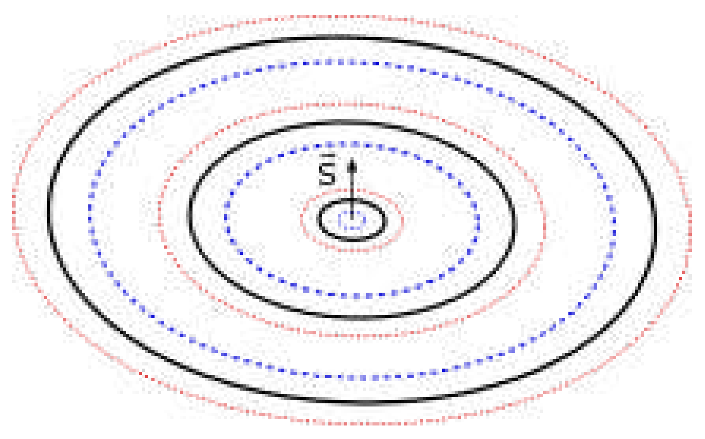
Figure 3.
Charge wave forces
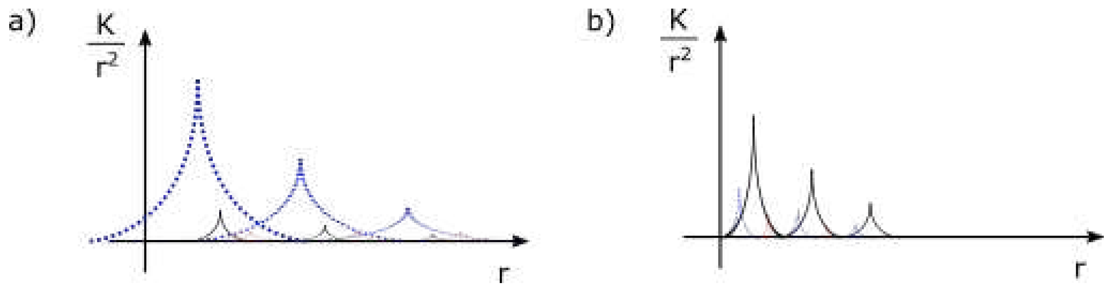
Figure 4.
Primary components of the Solar System (planet images source: Pixabay/OpenClipart-Vectors)
Figure 4.
Primary components of the Solar System (planet images source: Pixabay/OpenClipart-Vectors)
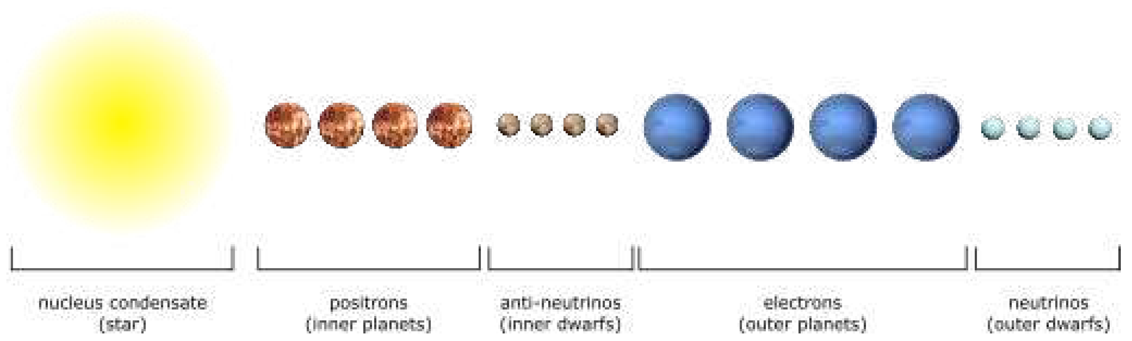
Figure 5.
a) stable C energy levels b) possible Solar System (U.C) energy levels
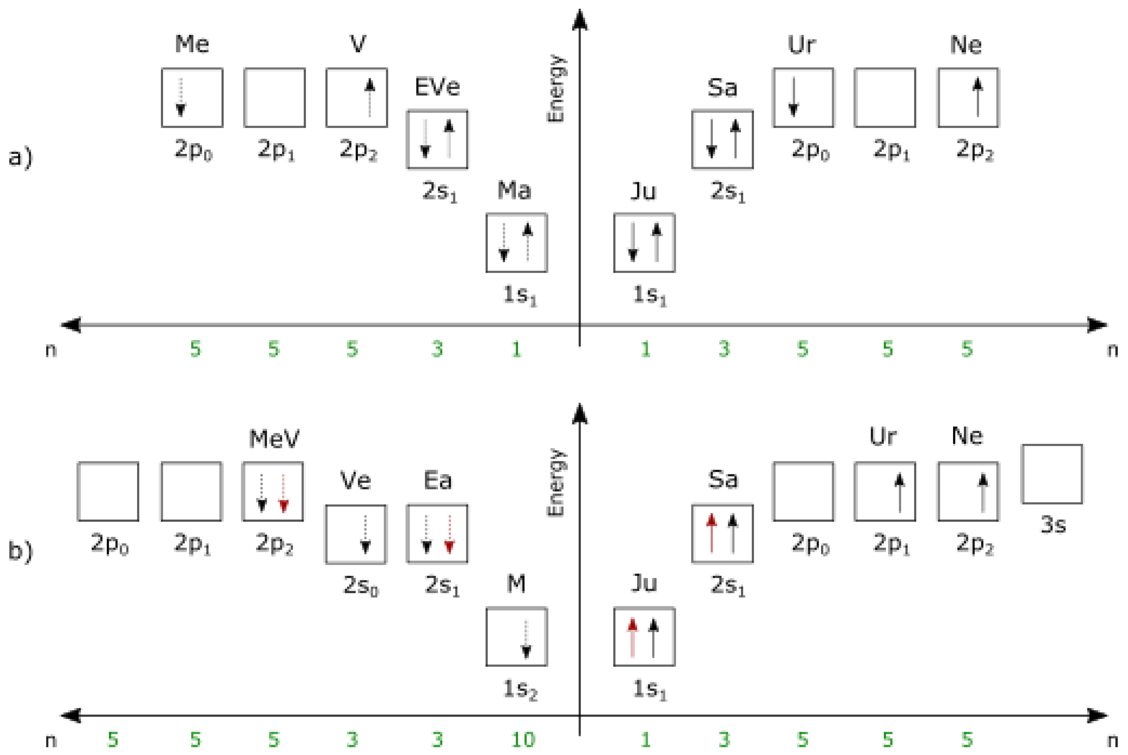
Figure 6.
Primary components of the TOI-178 System (planet images source: Pixabay/OpenClipart-Vectors)
Figure 6.
Primary components of the TOI-178 System (planet images source: Pixabay/OpenClipart-Vectors)
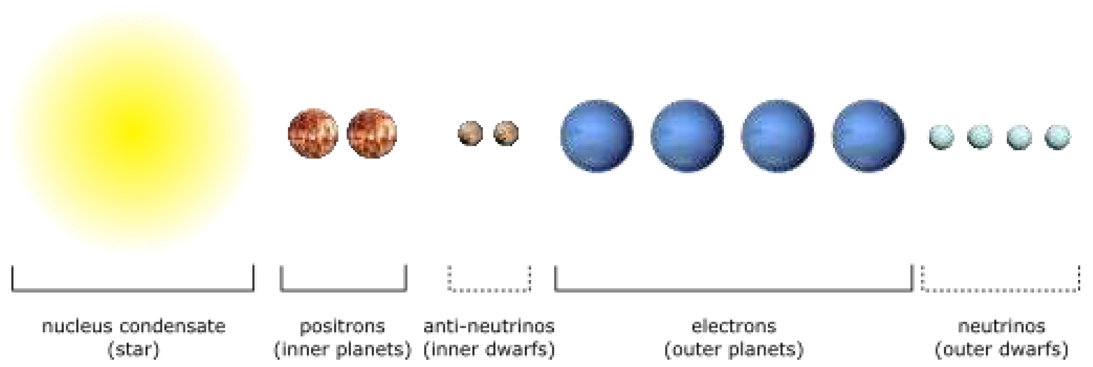
Figure 7.
left) internal rotation of the Sun, right) rotation of spiral galaxies
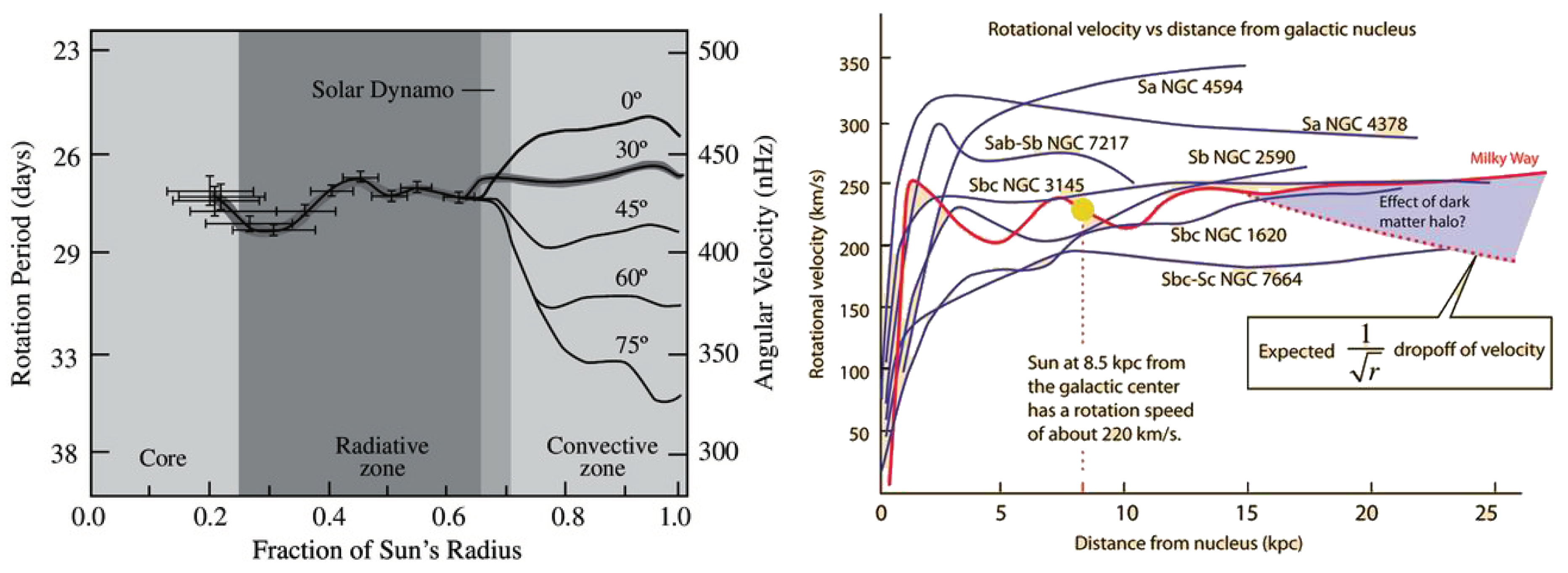
Figure 8.
Rotational velocities of the Sun
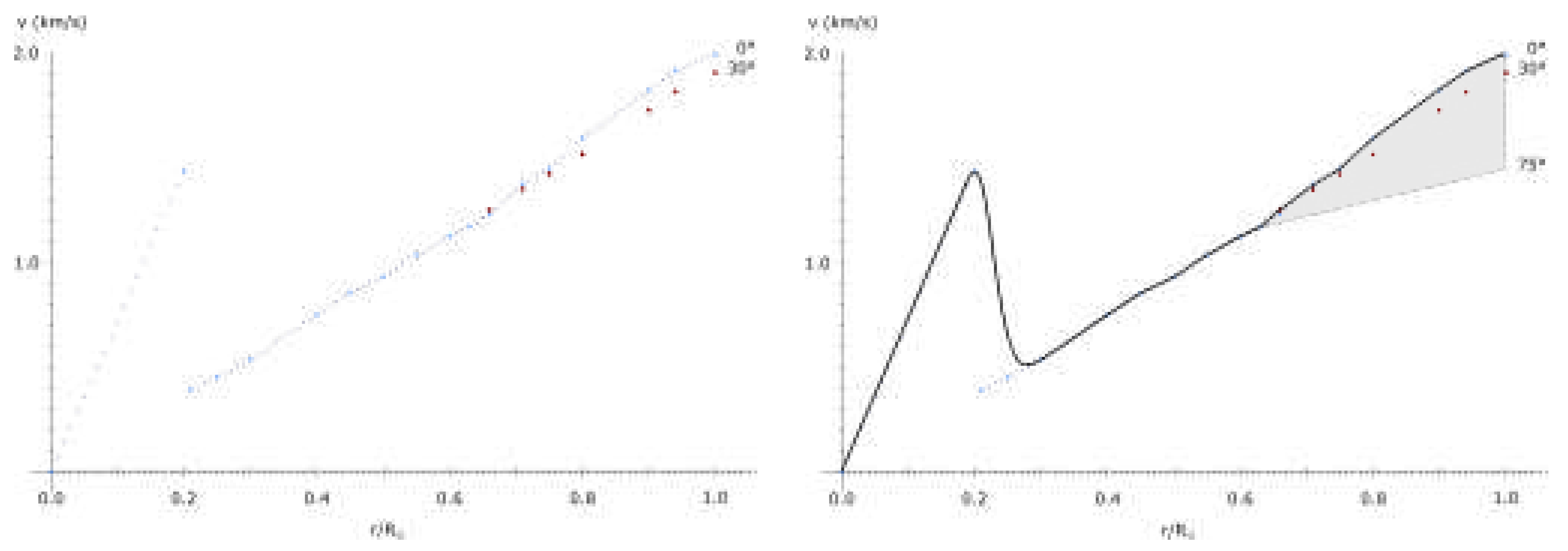
Figure 9.
Rotational velocities of the Sun and near corona
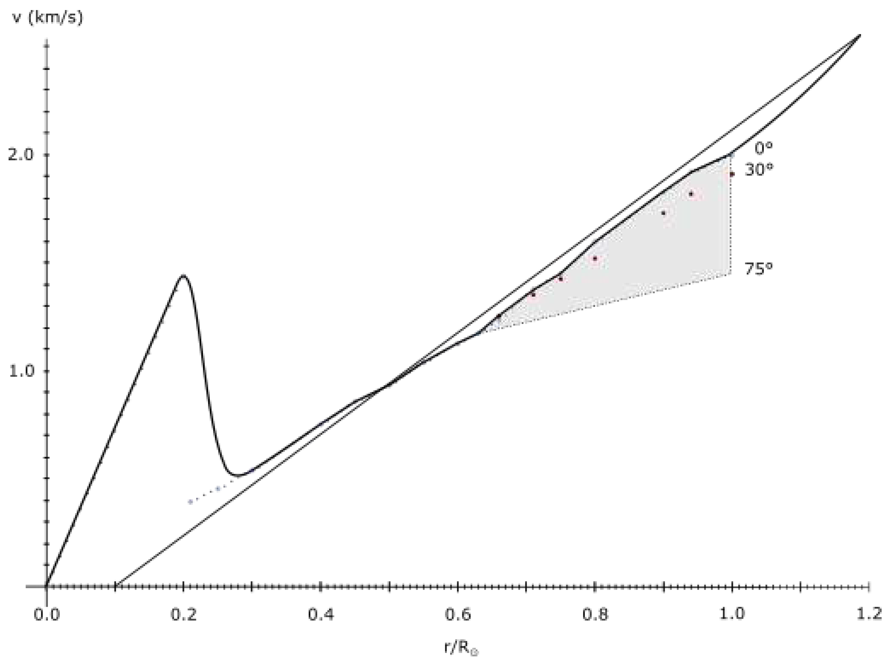
Figure 10.
Oscillation of the gravitational constant
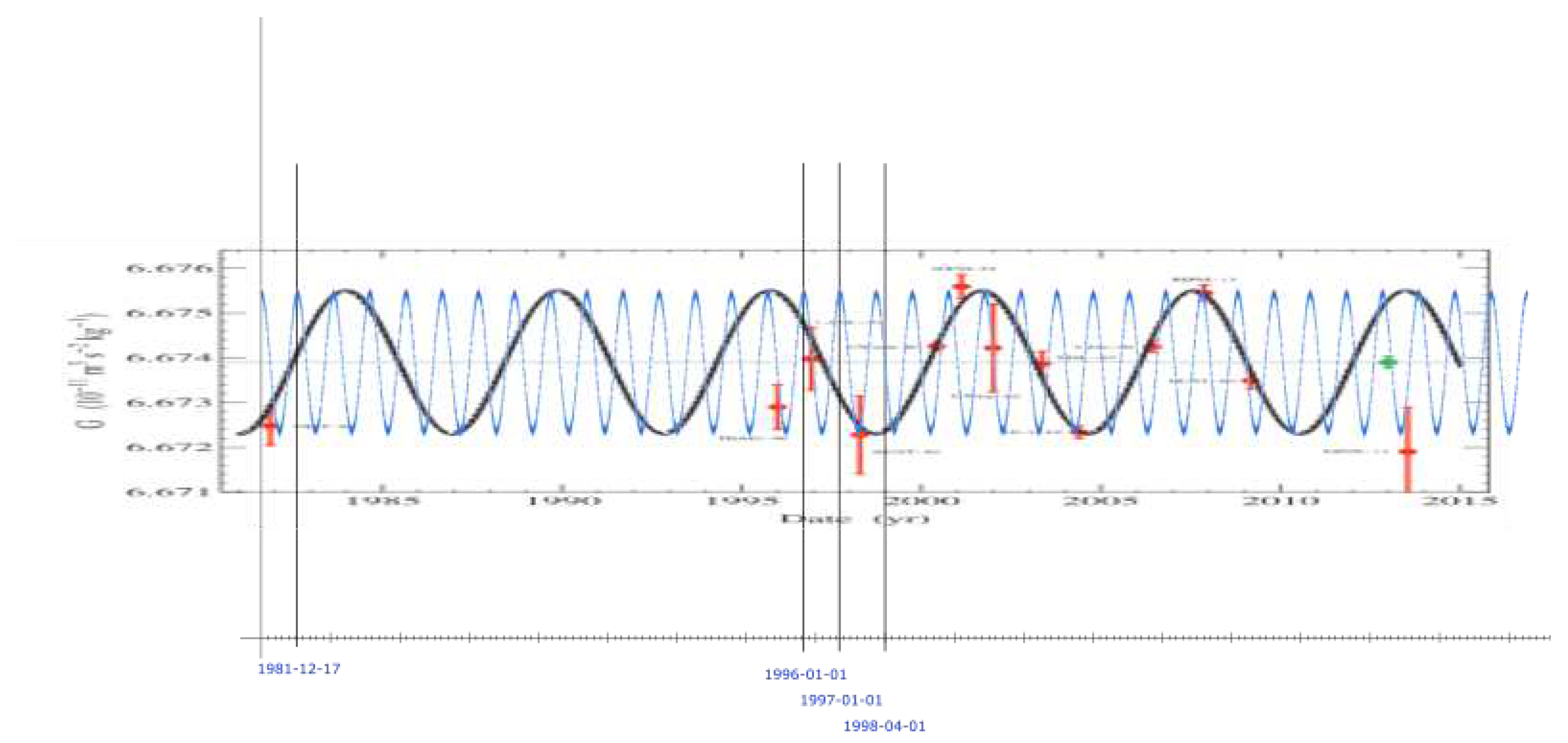
Figure 11.
Oscillation of the gravitational constant
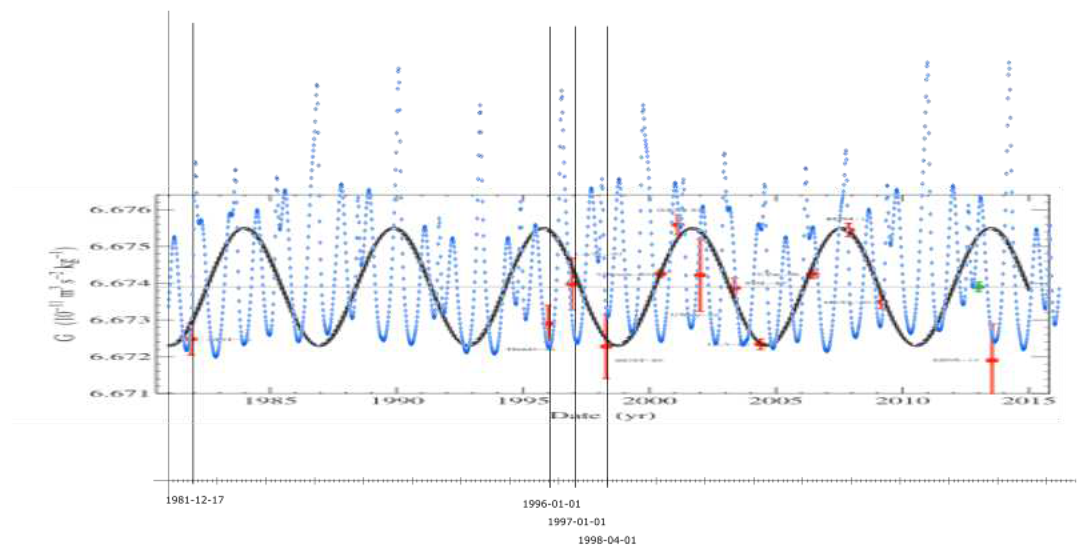
Figure 12.
Sun partitioning in: a) 6p4n state b) 4p6n state (R = radius in 6p4n state)
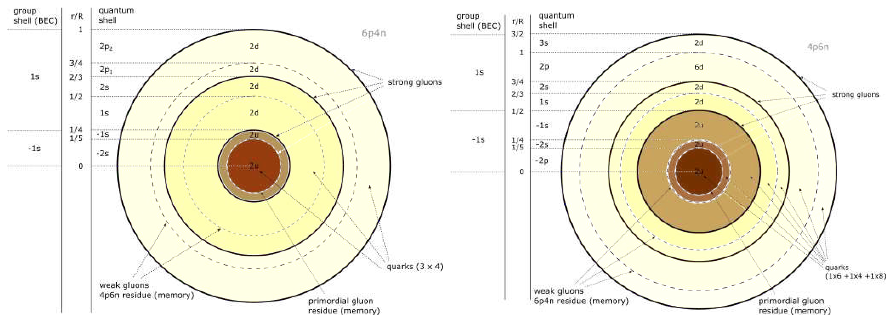
Figure 13.
Equatorial anisotropy of the Earth’s inner core
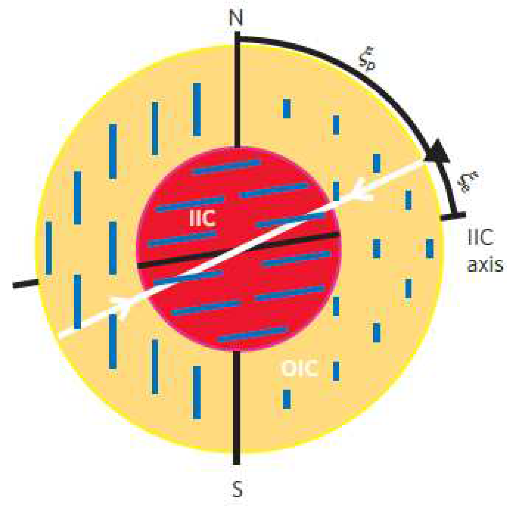
Figure 14.
Magnetic field of Jupiter, left) =0, right) =109 (N=2)
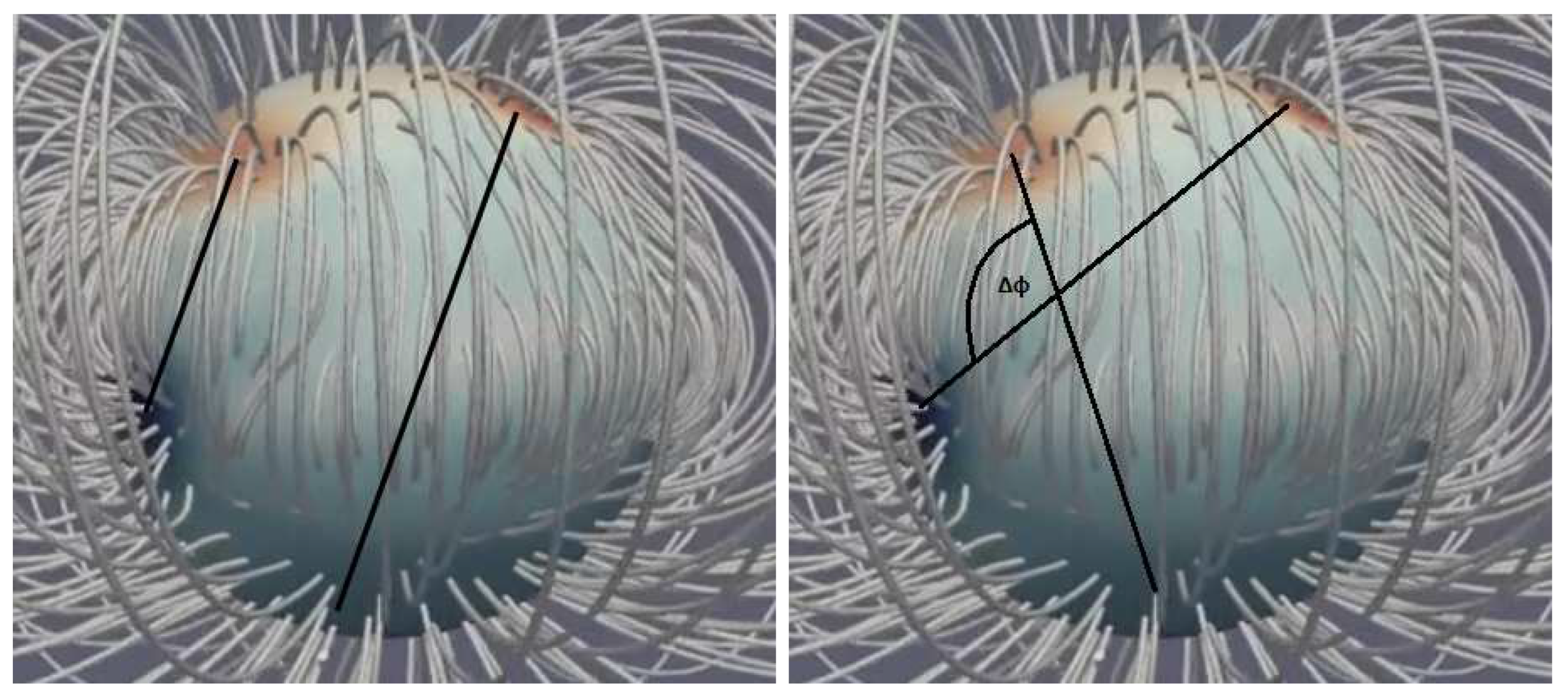
Figure 15.
Uranus’ magnetic field model
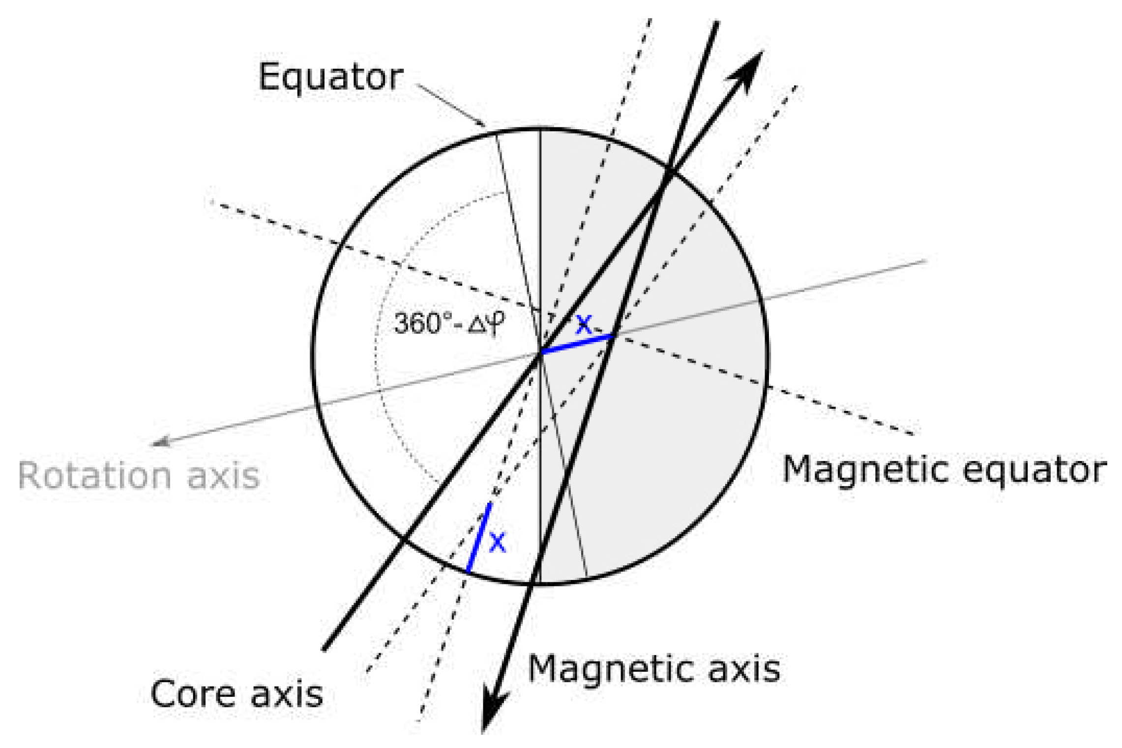
Figure 16.
Neptune’s magnetic field model
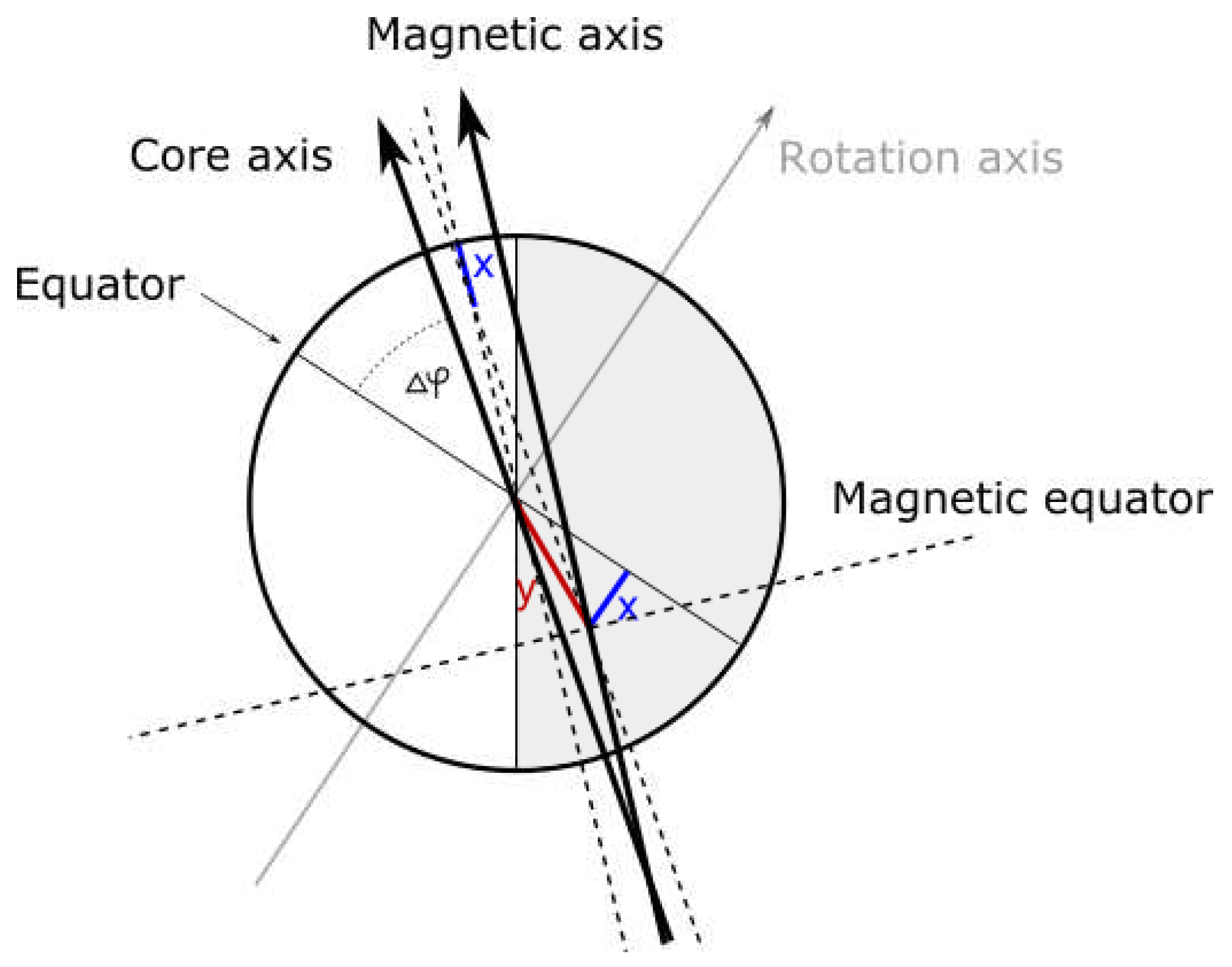
Figure 17.
Layers of Earth’s brain, superimposed on seismic velocities
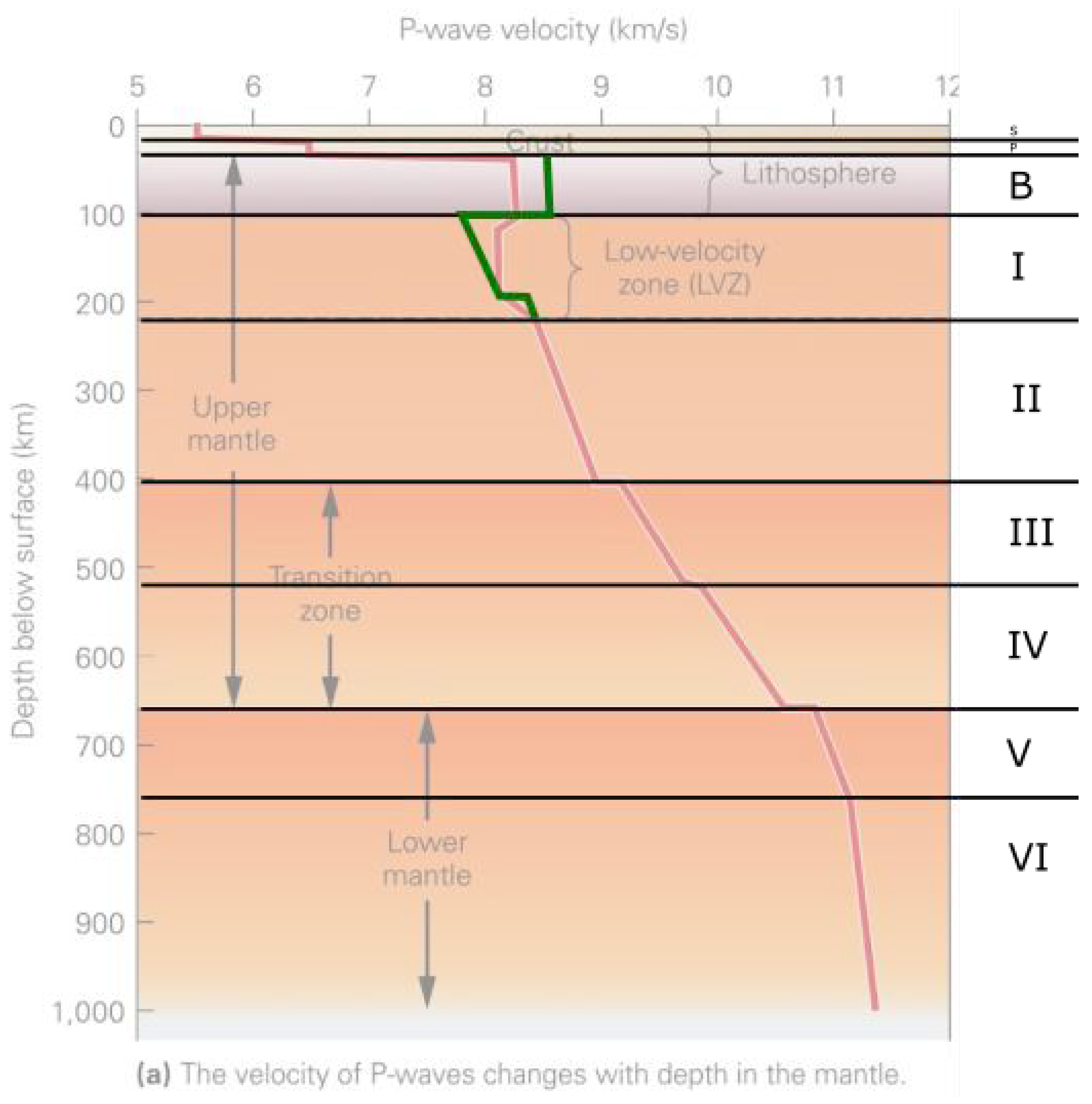
Figure 18.
The history of atmospheric CO concentration
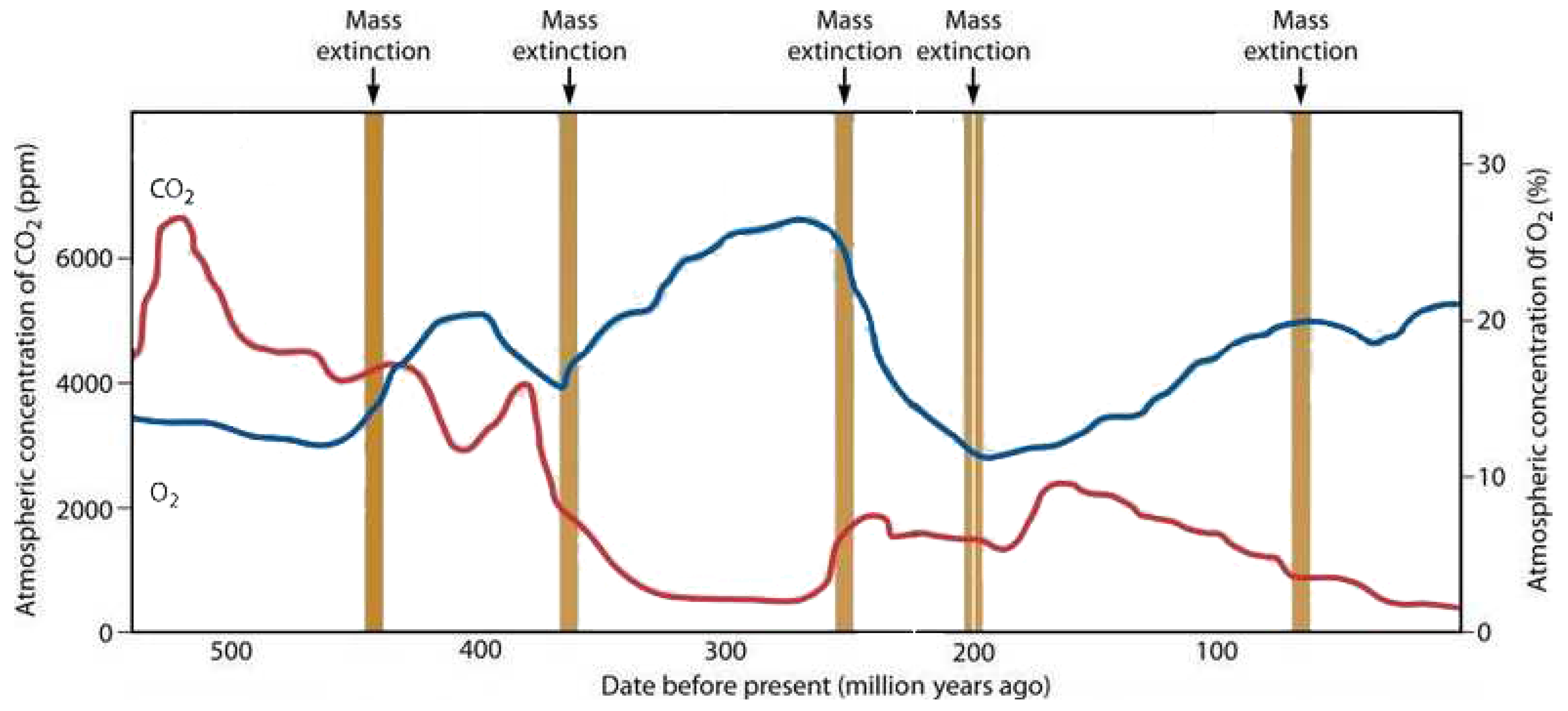
Figure 19.
CO pH minimum marker models a) and b) (blue dots = major extinction events, red = minor extinction events, on b) grey = icehouse periods, white = greenhouse periods)
Figure 19.
CO pH minimum marker models a) and b) (blue dots = major extinction events, red = minor extinction events, on b) grey = icehouse periods, white = greenhouse periods)
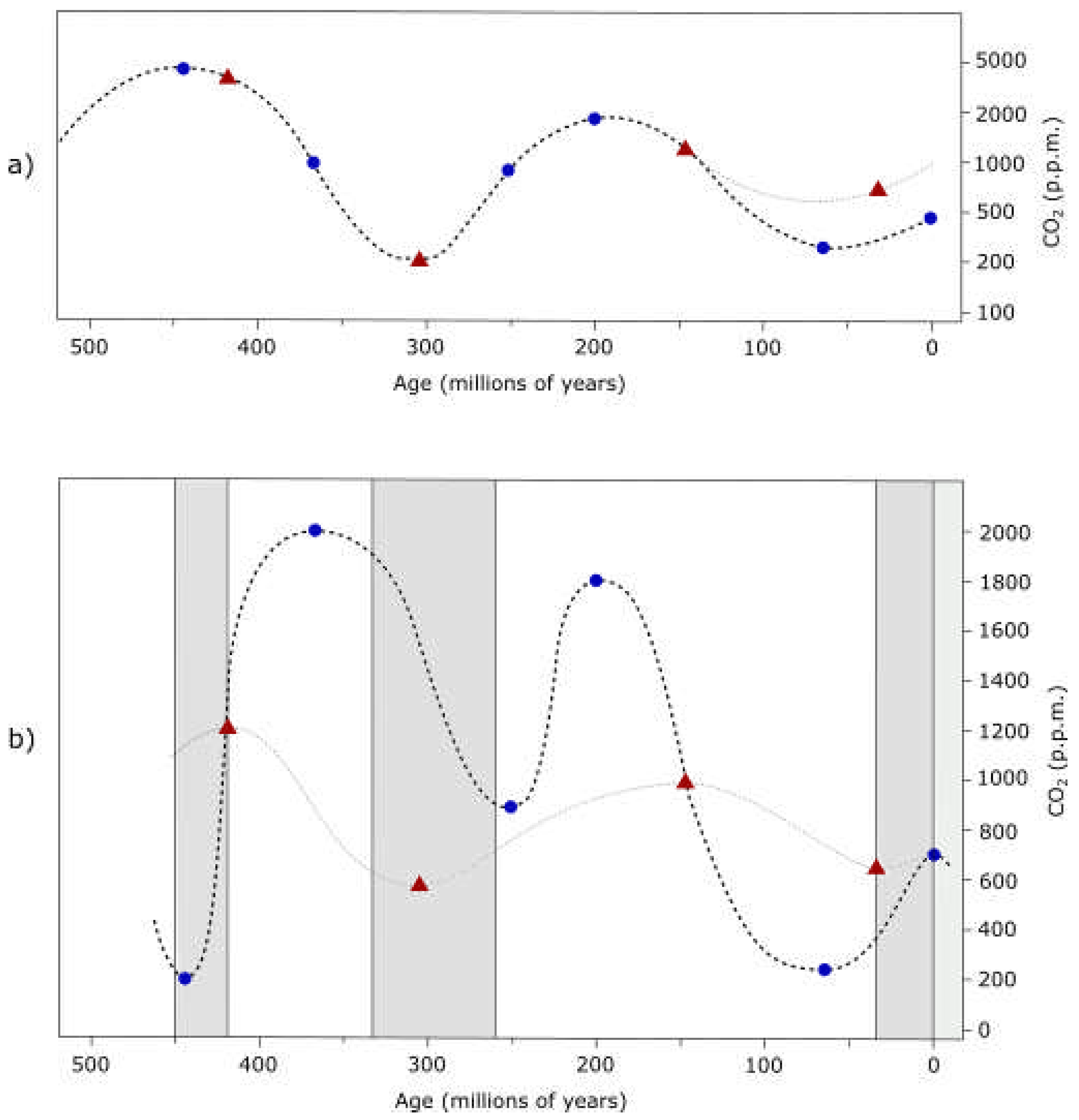
Figure 20.
Recent history of CO concentration
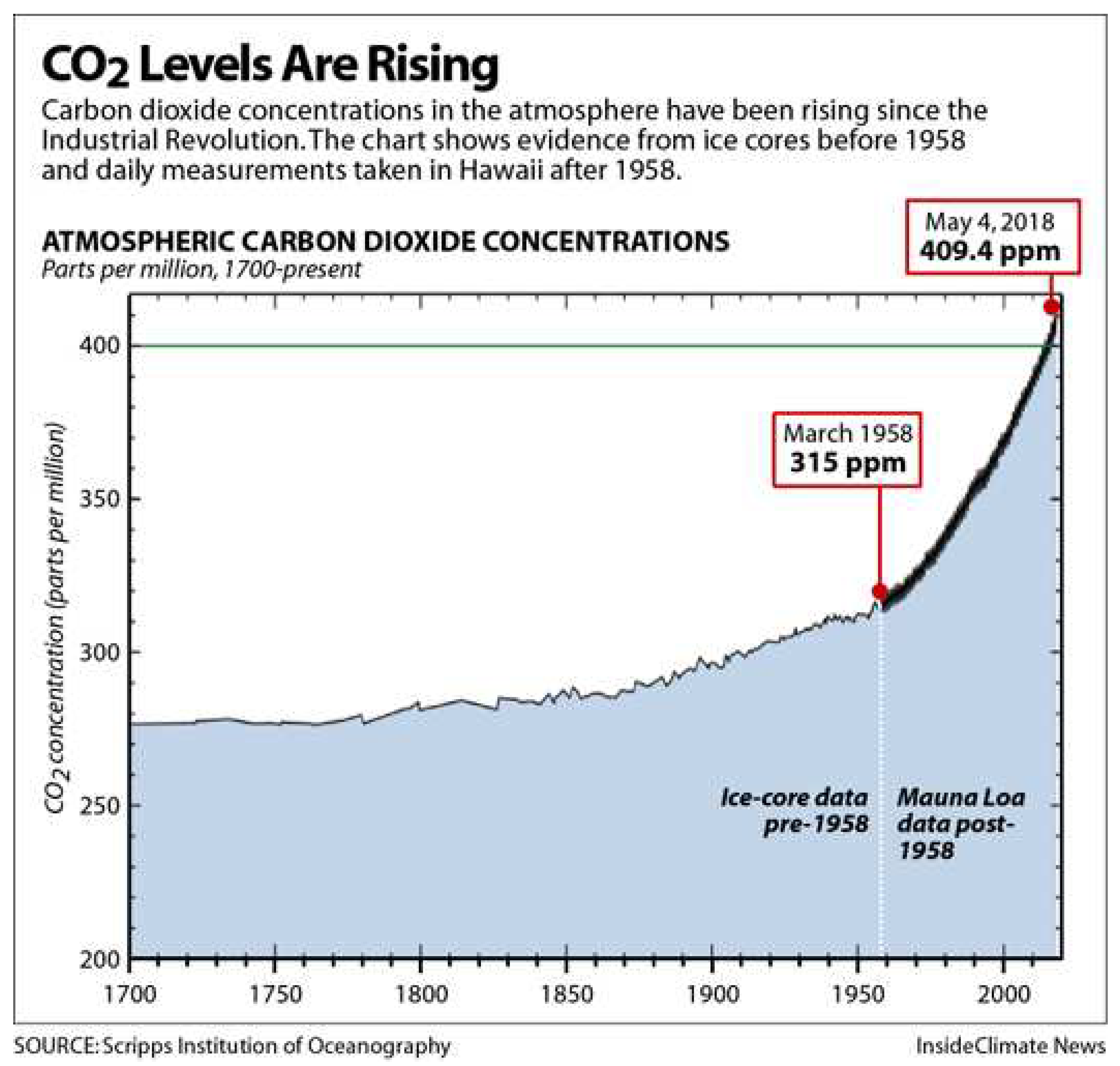
Figure 21.
Neutrino pulse due to decay rate increase
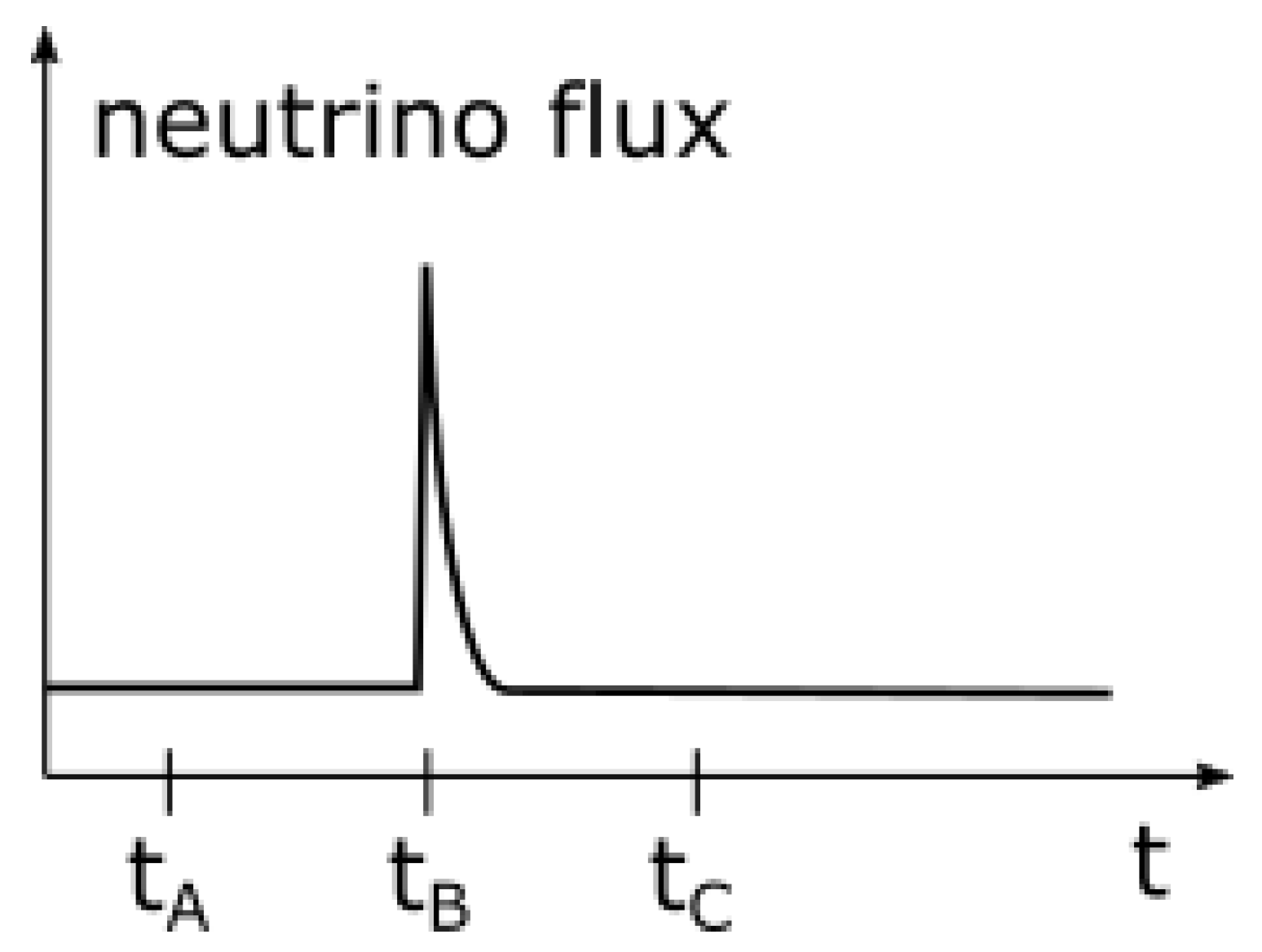
Figure 22.
Extinctions (left), spectral analysis (right)
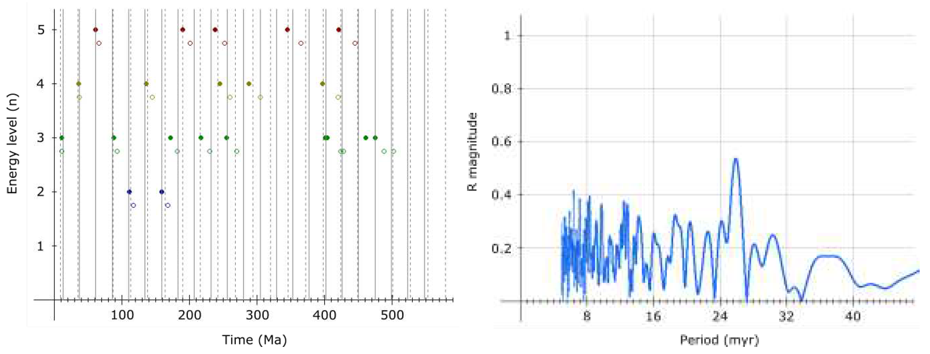
Figure 23.
Extinctions (left), spectral analysis (right)

Figure 27.
Correlation of major extinctions (left) with Earth’s mantle layers (right)
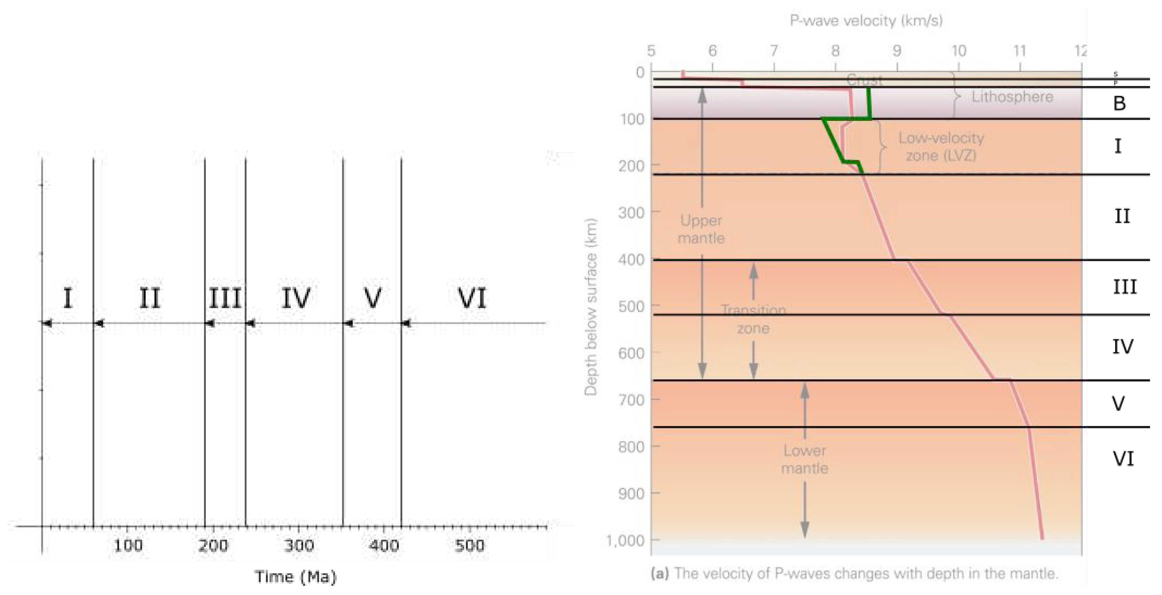
Table 1.
Commonly used constants.
| Description | Constant | Value |
| Neptune mass on scale 1 | M | 1.02413 * 10 kg |
| Neptune equivalent mass on scale 0 | M | ( 9.10938356 * 10 kg / 510998.9461 eV ) * ( 510998.9461 eV - 11.260288 eV ) = 9.109182827 * 10 kg |
| Neptune orbital velocity | v | 5430 m/s |
| Neptune spin velocity | s | 2660 m/s |
| Neptune radius on scale 1 | R | 24622000 m |
| Neptune equivalent radius on scale 0 | R | ( 24622000 m / 4495060000000 m ) * 70 * 10 m = 3.834298096 * 10 m |
| Solar System charge radius = Neptune orbital radius | r | 4495060000000 m |
| Sun mass | M | 1.988500 * 10 kg |
| Sun radius | R | 695735 km = 695735000 m |
| Earth mass | 5.9723 * 10 kg | |
| Carbon-12 atom mass | 1.992646547 * 10 g = 1.992646547 * 10 kg | |
| Carbon-12 charge radius = Carbon-10 charge radius | r | 70 pm = 70 * 10 m |
| Carbon-10 nucleus charge radius | 2.708 * 10 m | |
| Carbon-10 nucleus mass | 10.016853 u = 1.663337576 * 10 kg | |
| Standard speed of light | c = c | 2.99792458 * 10 m/s |
| Standard electron mass | M | 9.10938356 * 10 kg |
Table 3.
4th order period correlation with excursions
| cycle | years before present | correlated event |
| 0 | 0 | current events (extinction, climate change, ozone depletion, likely magnetic excursion or reversal, ...) |
| 1 | 9221.4 | Be enrichment in ice cores ≈9200 years ago[17] (hypothesized extreme solar storm event), Lake Michigan/Erie magnetic excursion 10-9 ka and 14-12 ka[18] |
| 2 | 18442.8 | Hilina Pali magnetic excursion 18.5 ka[19] |
| 3 | 27664.2 | Lake Mungo magnetic excursion 30780±520 - 28140±370 and ≈26000 years b.p.[20], Oruanui eruption ≈26.5 ka[21] |
| 4 | 36885.6 | Mono Lake magnetic excursion 36 - 30 ka[22] (34.5 ka[19]), Dome C/Vostok Be enrichment (likely due to excursion) ≈35 ka[23] |
| 5 | 46107.0 | Laschamp magnetic excursion 46.6±2.4 ka[24] (41.2 ka[19]), Neanderthals extinction |
| 6 | 55328.4 | ? |
| 7 | 64549.8 | Norwegian-Greenland Sea magnetic excursion 64.5 ka[19] |
| 8 | 73771.2 | Toba volcanic eruption ≈74000 years ago[25] |
Table 4.
Calculated gravity for outer planets
| n | planet | orbital velocity v (m/s) | orbital radius r (10 km) | total mass M (10 kg) | required total mass (10 kg) | calc. gravity g (m/s) | gravity (m/s) | acc. (m/s) |
| 5 | Neptune | 5430 | 4495.06 | 102.413 | 102.413 | 11.15 | 11.15 | 11.00 |
| 5 | Uranus | 6800 | 2872.46 | 86.813 | 127.976 | 8.92 | 8.87 | 8.69 |
| 3 | Saturn | 9680 | 1433.53 | 568.340 | 108.084 | 10.565 | 10.44 | 8.96 |
| 1 | Jupiter | 13060 | 778.57 | 1898.190 | 49.168 | 23.225 | 24.79 | 23.12 |
Table 5.
Calculated gravity for inner planets
| n | planet (mirror) | orbital velocity v (m/s) | orbital radius r (10 km) | total mass (10 kg) | required total mass (10 kg) | calc. gravity g (m/s) | gravity (m/s) |
| 5 | Mercury (Neptune) | 47360 | 57.91 | 0.330 | 0.33011 | 3.70 | 3.70 |
| 3 | Venus (Uranus) | 35020 | 108.21 | 4.868 | 0.14335 | 8.52 | 8.87 |
| 3 | Earth (Saturn) | 29780 | 149.6 | 5.972 | 0.12193 | 10.02 | 9.798 |
| 10 | Mars (Jupiter) | 24070 | 227.92 | 0.642 | 0.33006 | 3.70 | 3.71 |
Table 6.
Examples of discrete surface gravity and orbital distance for inner planets
| base | state | N/P | surface gravity/orbital distance examples |
| Carbon | 6p4n | 4/6 = 2/3 | Mercury 3.7 (0.25 MAU, n=5), Venus 8.87 (0.5 MAU, n=3), Earth 9.798 (0.66 MAU, n=3), Mars 3.71 (1 MAU, n=10) |
| Boron | 5p5n | 5/5 = 1 | Mercury B 3.32 (0.2 MAU, n=5), Venus/Earth A 5.25 (0.5 MAU, n=5), Earth B/Mars 6.43 (0.75 MAU, n=5) |
| Beryllium | 4p6n | 6/4 = 3/2 | Venus/Earth A 1.85 (0.25 MAU orbit, n=10), Earth B/Mars 37.1 (1 MAU, n=1) |
Table 7.
Obtained values for l, s and ℏ for outer planets
| n | conf. | l | s | planet | orbital vel. v (m/s) | orbital radius r (10 km) | spin vel. v (m/s) | spin radius R (km) | spin rot. period T (h) | calc. ℏ (Js) |
| 5 | 1e | 1 | 1/2 | Neptune | 5430 | 4495.06 | 2668 | 24622 | 16.11 | 1.3310 * 10 |
| 5 | 1e | 1 | 0 | Uranus | 6800 | 2872.46 | 2568 | 25362 | 17.24 | 1.3319 * 10 |
| 3 | 2e | 1 | 0 | Saturn | 9680 | 1433.53 | 9538 | 58232 | 10.656 | 1.3636 * 10 |
| 1 | 2e | 0 | 1 | Jupiter | 13060 | 778.57 | 12293 | 69911 | 9.9250 | 1.3817 * 10 |
Table 8.
Possible configuration of inner planets
| n | conf. | l | s | planet | total mass (10 kg) | orbital vel. v (m/s) | orbital radius r (10 km) | spin vel. v (m/s) | spin radius R (m) | calc. ℏ (Js) |
| 10 | 1e | 1 | 1/2 | Mars | 0.642 | 24070 | 227.92 | 27650 | 56044 | 4.3107 * 10 |
| 3 | 2e | 1 | 0 | Earth | 5.972 | 29780 | 149.6 | 28435 | 492971 | 4.3107 * 10 |
| 3 | 1e | 1 | 0 | Venus | 4.868 | 35020 | 108.21 | 45462 | 157195 | 4.3107 * 10 |
| 5 | 2e | 0 | 1 | Mercury | 0.330 | 47360 | 57.91 | 58980 | 6333 | 4.3107 * 10 |
Table 10.
Obtained k momentum for outer planets
| n | configuration | l | s | planet | |
| 5 | 1e | 1 | 1/2 | Neptune | |
| 5 | 1e | 1 | 0 | Uranus | |
| 3 | 2e | 1 | 0 | Saturn | 1 |
| 1 | 2e | 0 | 1 | Jupiter |
Table 11.
Possible quantization parameters and spin radii for inner planets
| n | conf. | l | s | planet | spin radius (m) | |
| 10 | 1e | 1 | 1/2 | Mars | 6477988 | |
| 3 | 2e | 1 | 0 | Earth | 1 | 4146215 |
| 3 | 1e | 1 | 0 | Venus | 3920325 | |
| 5 | 2e | 0 | 1 | Mercury | 4140950 |
Table 12.
Possible quantization parameters and spin radii for inner planets, with corrected h
| n | conf. | l | s | planet | spin radius (m) | |
| 10 | 1e | 1 | 1/2 | Mars | 713566 | |
| 3 | 2e | 1 | 0 | Earth | 1 | 456716 |
| 3 | 1e | 1 | 0 | Venus | 431833 | |
| 5 | 2e | 0 | 1 | Mercury | 456136 |
Table 13.
Standard particle candidates for planets (green = most likely)
| planet | relativistic mass M [10 kg] (v) | rest mass M candidates [10 kg] (c) | particle candidates (MeV/c) |
| Mercury | 0.330 (47.4 km/s) | 0.361 (19.34 km/s = Vesta orbit), 0.353 (16.76 km/s = Hygiea orbit), 0.383 (24.1 km/s = Mars orbit), 0.489 (35 km/s = Venus orbit) |
? (0.198), positron (0.511) |
| Venus | 4.868 (35.0 km/s) |
5.67 (17.905 km/s = Ceres orbit), 5.545 (16.76 km/s = Hygiea orbit) |
anti-down quark (≈4.8) |
| Earth | 5.972 (29.8 km/s) | 7.47 (17.905 km/s = Ceres orbit), 7.47 (17.89 km/s = Pallas orbit), 4.77 (-17.905 km/s = -Ceres orbit) |
anti-down quark (≈4.8) |
| Mars | 0.642 (24.1 km/s) | 1.076 (19.34 km/s = Vesta orbit), 0.383 (-19.34 km/s = -Vesta orbit), 0.461 (-16.76 km/s = -Hygiea orbit), 0.539 (-13.1 km/s = -Jupiter orbit) |
positron (0.511) |
| Jupiter | 1898.19 (13.1 km/s) | 1396 (-19.34 km/s = -Vesta orbit), 1293 (-17.905 km/s = -Ceres orbit), 1824 (-47.4 km/s = -Mercury orbit) |
D meson (1869), tau (1776.86), anti-charm quark (≈1275) |
| Saturn | 568.34 (9.7 km/s) |
491.4 (-19.34 km/s = -Vesta orbit), 477.7 (-17.905 km/s = -Ceres orbit) |
K meson (493.7) |
| Uranus | 86.813 (6.8 km/s) | 80.285 (-17.89 km/s = -Pallas orbit), 94.982 (16.76 km/s = Hygiea orbit) |
muon (105.658), strange quark (≈95) |
| Neptune | 102.413 (5.43 km/s) | 96.5 (-16.76 km/s = -Hygiea orbit) | muon (105.658), strange quark (≈95) |
Table 14.
Standard particle candidates for planets, with listed electric charges
| planet | configuration | particle species (charge) | total charge |
| Mercury | 2e | positron (1 e) | 2 e |
| Venus | 1e | anti-down quark (1/3 e) | 1/3 e |
| Earth | 2e | anti-down quark (1/3 e) | 2/3 e |
| Mars | 1e | positron (1 e) | 1 e |
| Jupiter | 2e | anti-charm quark (2/3 e) | 4/3 e |
| Saturn | 2e | K meson (1 e) | 2 e |
| Uranus | 1e | strange quark (1/3 e) | 1/3 e |
| Neptune | 1e | strange quark (1/3 e) | 1/3 e |
Table 15.
Standard particle candidates for planets (p1, p2, p3, p4, p5 hypothetical)
| planet | mass M [10 kg] | particle candidates (MeV/c) |
| Mercury | 0.330 | 1 x positron (0.511), 1 x p1 (≈0.34) |
| Venus | 4.868 | 1 x anti-down quark (≈4.8) |
| Earth | 5.972 | 1 x anti-down quark (≈4.8) + 1 x positron (0.511), 1 x anti-down quark (≈4.8) + 1 x up quark (1.2) |
| Mars | 0.642 | 1 x positron (0.511) + 1 x p1 (≈0.34), 2 x p1 (≈ 2 x 0.34), 1 x positron (0.511) + 1 x p2 (≈0.17) |
| Jupiter | 1898.19 | 1 x tau (1776.86), 2 x p3 (≈ 2 x 10¹³) |
| Saturn | 568.34 | 2 x muon (2 x 105.658), 2 x p4 (≈ 2 x 253.3), 1 x p5 |
| Uranus | 86.813 | 1 x muon (105.658) |
| Neptune | 102.413 | 1 x muon (105.658) |
Table 16.
Sum of outer charge
| configuration | charge sum [e] |
| 1 x tau, 1 x p5, 1 x muon, 1 x muon | -4 |
| 1 x tau, 2 x muon (or 2 x p4), 1 x muon, 1 x muon | -5 |
| 2 x p3, 1 x p5, 1 x muon, 1 x muon | -5 |
| 2 x p3, 2 x muon (or 2 x p4), 1 x muon, 1 x muon | -6 |
Table 17.
Calculated neutral and current radii, compared to measured R
| N | n | planet | M (kg) | r (10 km) | s | p | () | neutral R (km) | current R (km) | R (km) |
| 2 | 5 | Neptune | 1.02413 * 10 | 4495.06 | 1 | 2 | 36.7084 | 24764 | 24764 | 24764 |
| 2 | 5 | Uranus | 8.6813 * 10 | 2872.46 | 1 | 1 | 233.1511 | 25703 | 25559 | 25559 |
| 2 | 3 | Saturn | 5.6834 * 10 | 1433.53 | 2 | 1 | 0.2 | 60806 | 60268 | 60268 |
| 1 | 1 | Jupiter | 1.89819 * 10 | 778.57 | 2 | 1 | -0.847 | 68848 | 71492 | 71492 |
| 2 | 5 | Mercury | 3.3011 * 10 | 57.91 | 2 | 2 | 172.3047 | 2555.7 | 2439.7 | 2439.7 |
| 2 | 3 | Venus | 4.8675 * 10 | 108.21 | 1 | 0 | 0 | 6051.8 | 6051.8 | 6051.8 |
| 2 | 3 | Earth | 5.9723 * 10 | 149.60 | 2 | 1 | 90.3135 | 6284.72 | 6378.14 | 6378.14 |
| 1 | 10 | Mars | 6.4171 * 10 | 227.92 | 1 | 2 | -91.9957 | 3394.1 | 3396.2 | 3396.2 |
Table 18.
Correlation of outer and inner planets, in case of anti-aligned and aligned entanglements
| planet | normalized () | entanglement (anti-aligned) | entanglement (aligned) |
| Neptune | (5 * 36) % 360 = 180 | Venus | Mercury |
| Uranus | (5 * 234) % 360 = 90 | Mars | Earth |
| Saturn | (5 * 0) % 360 = 0 | Mercury | Venus |
| Jupiter | (5 * 0) % 360 = 0 | Mercury | Venus |
Table 20.
Orbital velocities of time and event horizon dimensions
| n | Planet | i | j | v (km/s) | v km/s (entanglement) | (current value) | v (entanglement) km/s | (neutron correction) | v (entanglement) km/s |
| 4 | Mercury | 2 | -1 | 47.36 | 5.47 (Neptune) | -2 * 10 = -0.04 | 12.033 (Jupiter) | +4.73 | 16.77 (Hygiea) |
| 3 | Venus | 1 | 0 | 35.02 | 6.78 (Uranus) | +2 * 10 = +0.02 | 16.63 (Hygiea) | +1.275 | 17.9 (Ceres) |
| 2 | Earth | 0 | 1 | 29.78 | 9.66 (Saturn) | +2 * 10 = +0.02 | 19.55 (Vesta) | -1.66 | 17.88 (Pallas) |
| 1 | Mars | -1 | 2 | 24.07 | 13.08 (Jupiter) | -2 * 10 = -0.02 | 24.07 (Mars) | -4.73 | 19.34 (Vesta) |
Table 22.
CO pH minimum marker models
| year [mya] | a) CO [ppm] | b) CO [ppm] | c) CO [ppm] | d) CO [ppm] | e) CO [ppm] |
| 444 | 3800 | 200 | 2000 | 3800 | 2000 |
| 370 | 1000 | 2000 | 1000 | 1800 | 1200 |
| 252 | 800 | 900 | 800 | 800 | 800 |
| 201 | 1800 | 1800 | 1800 | 1800 | 600 |
| 66 | 250 | 250 | 250 | 300 | 500 |
| 0 | 450 | 700 | 750 | 800 | 450 |
Table 23.
Calculated impact dates and possible impactors (2nd order = lower energy)
| model | CO [ppm] | year of impact | associated impactor (diameter) | impactor closest approaches | 2nd order impactor (diameter) |
| a), e) | 450 | 2029 | 99942 Apophis (≈375 m) | 2029, 2065 | |
| b) | 700 | 2066 | 99942 Apophis (≈375 m) | 2029, 2065 | |
| c) | 750 | 2071 | 1866 Sisyphus (≈7 km) | 2058, 2071 | 2000 SG (37 m) |
| d) | 800 | 2075 | 162173 Ryugu (≈1 km) | 2076 |
Table 26.
Extinction events dataset 1, sources: *, a, b, c, d, e, f, g, h
| energy level | extinction events [mya] | extinction events (t), age corrected [mya] |
| 5 | 66*, 201.3*, 252.2*, 365, 445 | 61.986, 190.208, 238.316, 345.385, 421.148 |
| 4 | 37.8*, 145*, 260, 305, 420 | 36.206, 136.774, 245.993, 288.3, 397.519 |
| 3 | 11.6*, 93.9*, 182.7*, 230, 270, 424e, 428, 488, 502 | 11.402, 88.465, 172.88, 217.463, 255.844, 401.469, 404.42, 461.48, 475.257 |
| 2 | 117, 168.3* | 111.194, 159.702 |
Table 32.
Comparison of weak evolution periods and mantle layers, sources: a, b
| i | Period of weak evolution T [My] | Normalized period of weak evolution T | Corresponding mantle layer thickness D [km] | Normalized layer thickness D |
| 5 | 421.348 - 352.461 = 68.887 | 0.163 | 780 - 660 = 120 | 0.176 |
| 4 | 352.461 - 238.041 = 114.42 | 0.272 | 660 - 520 = 140 | 0.206 |
| 3 | 238.041 - 190.308 = 47.733 | 0.113 | 520 - 410 = 110 | 0.162 |
| 2 | 190.308 - 61.986 = 128.322 | 0.305 | 410 - 220 = 190 | 0.279 |
| 1 | 61.986 - 0 = 61.986 | 0.147 | 220 - 100 = 120 | 0.176 |
Table 33.
Correlation of weak evolution periods and mantle layers (or, major extinctions and discontinuities)
Table 33.
Correlation of weak evolution periods and mantle layers (or, major extinctions and discontinuities)
| i | Period of weak evolution T [My] | Normalized period of weak evolution T | Corresponding mantle layer thickness D [km] | Normalized layer thickness D |
| 5 | 421.3 - 352.5 = 68.8 | 0.163 | 780 - 670 = 110 | 0.162 |
| 4 | 352.5 - 245.8 = 106.7 | 0.253 | 670 - 500 = 170 | 0.250 |
| 3 | 245.8 - 190.3 = 55.5 | 0.132 | 500 - 410 = 90 | 0.132 |
| 2 | 190.3 - 62.0 = 128.3 | 0.305 | 410 - 200 = 210 | 0.309 |
| 1 | 62.0 - 0 = 62.0 | 0.147 | 200 - 100 = 100 | 0.147 |
Table 34.
Correlation of weak evolution periods and mantle layers, using uncorrected ages
| i | Period of weak evolution T [My] | Normalized period of weak evolution T | Corresponding mantle layer thickness D [km] | Normalized layer thickness D |
| 5 | 445.2 - 372.2 = 73.0 | 0.164 | 780 - 670 = 110 | 0.162 |
| 4 | 372.2 - 259.8 = 112.4 | 0.252 | 670 - 500 = 170 | 0.250 |
| 3 | 259.8 - 201.4 = 58.4 | 0.131 | 500 - 410 = 90 | 0.132 |
| 2 | 201.4 - 66.0 = 135.4 | 0.304 | 410 - 200 = 210 | 0.309 |
| 1 | 66.0 - 0 = 66.0 | 0.148 | 200 - 100 = 100 | 0.147 |
Table 35.
Allowed orbitals of the Moon
| entanglement | r (km) | r (km) |
| Mercury | 57910000 | 100392 |
| Venus | 108210000 | 187591 |
| Earth | 149600000 | 259344 |
| Mars | 227920000 | 395118 |
Table 36.
Correlation of orbital and Schwarzschild radii
| Planet | R | R | Schwarzschild radius r (10 km) | current orbital radius (10 km) | orbital radius (MAU) |
| Mars | R | 1/2 R | 228.52 | 227.92 | 1 |
| Earth | 2/3 R | 1/2 R | 151.59 | 149.6 | 2/3 |
| Venus | 2/3 R | 1/5 R | 107.00 | 108.21 | 1/2 |
| Mercury | 2/5 R | 1/5 R | 57.81 | 57.91 | 1/4 |
Table 37.
Gravitational profile of the primordial Sun
| n | r/R | note | space velocity v (km/s) | space velocity v (km/s) | matter velocity v (m/s) | orbital radius r (km) | calculated gravity g (m/s) | calculated gravity g (m/s) | gravity g (vr product) m/s |
| 1 | 1 | Convective disc. | 436.602565 | 436.602565 | 1969.239615 | 695700 | 274 | 274 | 200 (1*10) |
| 1 | 3/4 | 4p6n disc. | 283.581685 | 286.551447 | 1508.068146 | 521775 | 154.125 | 157.37 | 150 (0.75 *10) |
| 1 | 2/3 | Radiative disc. | 234.100417 | 230.556106 | 1248 | 459162 | 119.3544 | 114.61 | 132 (0.66 * 10) |
| 1 | 1/2 | 4p6n disc. | 154.362317 | 151.266563 | 945.454545 | 347850 | 68.5 | 65.78 | 100 (0.5 * 10) |
| 1 | 2/5 | weak | 110.452683 | 108.233652 | 756.363636 | 278280 | 43.84 | 42.1 | 80 (0.4 * 10) |
| 1 | 1/4 | Outer core disc. | 54.575321 | 91.901023 | 1396 | 173925 | 17.125 | 48.56 | 50 (0.25 * 10) |
| 1 | 1/5 | Inner core disc. = r | 39.050921 | 74.602949 | 1437.401179 | 139140 | 10.96 | 40 | 40 (0.2 * 10) |
Table 40.
Grouping of elements
| n | shell (alt shell) | entanglement | elements | total elements = 2n |
| 1 | K | - | 1-2 (H - He) | 2 |
| 2 | L | Q | 3-10 (Li - Ne) | 8 |
| 2 | L (Q) | L | 11-18 (Na - Ar) | 8 |
| 3 | M | P | 19-36 (K - Kr) | 18 |
| 3 | M (P) | M | 37-54 (Rb - Xe) | 18 |
| 4 | N | O | 55-86 (Cs - Rn) | 32 |
| 4 | N (O) | N | 87-118 (Fr - Og) | 32 |
Disclaimer/Publisher’s Note: The statements, opinions and data contained in all publications are solely those of the individual author(s) and contributor(s) and not of MDPI and/or the editor(s). MDPI and/or the editor(s) disclaim responsibility for any injury to people or property resulting from any ideas, methods, instructions or products referred to in the content. |
© 2023 by the authors. Licensee MDPI, Basel, Switzerland. This article is an open access article distributed under the terms and conditions of the Creative Commons Attribution (CC BY) license (http://creativecommons.org/licenses/by/4.0/).
Copyright: This open access article is published under a Creative Commons CC BY 4.0 license, which permit the free download, distribution, and reuse, provided that the author and preprint are cited in any reuse.
supplementary.zip (5.70KB )
Submitted:
12 July 2023
Posted:
19 July 2023
Read the latest preprint version here
Alerts
supplementary.zip (5.70KB )
This version is not peer-reviewed
Submitted:
12 July 2023
Posted:
19 July 2023
Read the latest preprint version here
Alerts
Abstract
Origin, mechanics and properties of the Solar System are analysed in the framework of the Complete Relativity theory (by the same author). According to Complete Relativity, everything is relative. Any apparent absolutism (notably invariance to scale of dimensional constants, absolute elementariness, invariance to time) is an illusion stemming from limits imposed by [or on] polarized observers that will inevitably lead to misinterpretation of phenomena (another illusion) occurring on non-directly observable scales or even on observable but distant scales in space or time. If everything is relative, reference frames will exist where particles are planets and where planets are living beings. Earth is, therefore, analysed here in more detail, both as a particle and, as a living evolving being (of, hypothesized, extremely introverted intelligence). The analysis confirms the postulates and hypotheses of the theory (ie. existence of discrete vertical energy levels) with a significant degree of confidence. During the analysis, some new hypotheses have emerged. These are discussed and confirmed with various degrees of confidence. To increase confidence or refute some hypotheses, experimental verification is necessary. Main conclusions that stem from my research and are further confirmed in this paper are: universes are, indeed, completely relative; Solar System is a scaled (inflated, in some interpretations) Carbon isotope with a nucleus in a condensed (bosonic) state and components in various vertically excited states; life is common everywhere, albeit extroverted complex forms are present on planetary surfaces only during planetary neurogenesis; anthropogenic climate change is only a part (trigger from one perspective) of bigger global changes; major extinction events on a surface of a planet are relative extinctions, a regular part of transformation and transfer of life in the process of planetary neurogenesis.
Keywords:
Subject: Physical Sciences - Astronomy and Astrophysics
1. Introduction
Here I hypothesize that the Solar System is either a large scale C atom (10-Carbon isotope) or a superposition of such atoms in a relatively special state and provide evidence for the equivalence of large (U) scale systems with standard (U) scale systems through the analysis of the Solar System in the context of Complete Relativity[1] (CR).
I hypothesize that structure of planetary systems is a result of inflation of gravitational maxima from standard scale atoms, likely in the events of annihilation at relative event horizons (gravitational maxima) of a particular scale.
I propose that, in this process, the electro-magnetic component of the general force has been exchanged with the neutral gravitational component resulting in the dominance of gravity over electro-magnetic force at this scale.
However, I also propose that such exchange is natural on standard scale - atoms are cycling between polarized and neutral states (although durations in particular states might be inverted between scales).
In any case, the hypothesized equivalence between the Solar System and the C atom should be taken relative.
Implications of discrete vertical energy levels [and CR in general] on nature are large and particularly affect the understanding of life. Existence of these levels is required for conservation of relativity but one consequence is relativization of components of living beings (ie. living tissue, blood, etc.) between scales - they operate on different timescales and generally have different composition. In example, standard blood (blood of U scale), scaled to U scale will not be the same substance simply containing zillion extra standard cells, rather, to an U scale observer it will appear much different. Indeed, what I will consider the blood of a planet is commonly interpreted as magma. Thus, the planets can be living beings and here I will analyse Earth not only as a particle but as an evolving living being.
2. Constants
Table 1 shows commonly used constants in the paper.
The values of planetary constants are taken from NASA Planetary Fact Sheet[2].
3. Definitions
Definitions of terms and expressions that may be used in the paper. Note that these may be different than standard or common definitions in everyday use.
Some terms in use in this paper have been defined in CR and reader should be familiar with these (and CR in general) if the aim is to understand this paper properly.
3.1. Elementary charge
Elementary particles, relative to a universe of a particular scale, are generally polarized.
Physical interpretation (manifestation) of polarization is dependable on environment, but any elementary particle can be interpreted as a more or less evolved graviton (as defined in CR).
In case its electro-magnetic component is dominant, the particle is electrically charged and represents a relative electric monopole.
However, electric component is generally a sum of multiple constituent charge quanta, typically 2 quanta of identical charge and 1 quantum of opposite (anti) charge, which are strongly entangled (there are no absolute monopoles). Spin momentum of charge is quantized, by a relative constant (ℏ) - a quantum of momentum.
Suppose the spin momentum of each is equal to 1/2 ℏ in value, and spins of two dominant charges are perpendicular to each other (having a [fixed] phase difference of /2 degrees). Two dominant charges now have a total magnetic spin momentum:
Total spin momentum of the particle is thus:
If the S (anti) charge momentum is perpendicular to S, the value of total spin momentum is:
Due to fixed /2 phase and equal value, influence of components of S on the orientation [of the momentum projection] cancel (the two components are fermions in the same quantum energy level, so their projections cannot both be oriented in the same direction), and the orientation of the projection of the momentum S on the axis of quantization will depend solely on the orientation of momentum S.
With the applied magnetic field, projection of the momentum on the magnetic axis (ie. z) will thus be oriented either up or down:
This is a typical spin momentum of standard charges such as electrons and protons.
Figure 1 a) shows charge in a collapsed state (as a particle) with acquired (coupled) real mass m, charge radii r, r (corresponding to momenta S and S, respectively) and radius of imaginary mass r, here having a momentum aligned with S.
Its momentum is quantized by ℏ, electric charge by e and gravitational force by . The private space of such particle may be, depending on a reference frame, characterized either by properly scaled gradients or averages, of electric permittivity () and magnetic permeability () - or pressure and density.
With a decrease in environmental pressure (em/gravitational field interactions) a quantum may split into smaller quanta (which remain strongly entangled), spreading as far as possible (the range is finite and determined by the mass of smaller quanta - or environmental pressure on that scale), with a wave-like distribution of potential. Figure 2 illustrates such relatively unbound, free charge. Total momentum is the sum of individual momenta (and equal to original momentum of the particle in case of isotropic effect). With the splitting, the quantum of energy will decouple from real mass m unless the splitting is synchronized with the dilution or explosion of mass m where individual quanta of m are of appropriate scale and momenta to couple with individual quanta of img mass.
Figure 3 a) shows one interpretation of strength of forces of a wave with distance from centre (black = gravitational force, blue and red = electric force). Now each component (maximum) of a wave, starting from outer ones, can be excited independently, can change spin, merge with adjacent maxima and form moon charges.
This allows the charge to interact (interfere) with itself in certain reference frames.
However, if components are strongly entangled in a particular reference frame, entanglement will be conserved with any interaction - the waveform may simply collapse (localize) into corpuscular form.
Figure 3 b) shows how the private space of the same particle can be modified by interaction with another particle - essentially, the electric force has been exchanged for gravitational force. Such interaction may also collapse the wave into a particle with moon charges, where the number of moons depends on the equilibrium point of interaction (difference in energy of interacting particles).
Note that it is possible for the effect to be strongly localized - local space may be modified to attenuate one force and strengthen the other, while particles outside that space may not feel such [degree of] change.
3.1.1. Equilibrium and nature of forces
Equilibrium state of 3 components of charge is maintained through angular momenta. Due to rotation of local space, general force is a centripetal force and in stable orbitals equal to centrifugal force.
In case of a completely neutral (gravitational) force:
This is established when angular velocity of the orbiting body and angular velocity of space (effective graviton, or gravitational field tube) become equal:
If the body increases velocity (v > v), centrifugal force becomes greater than gravitational force and now acts as a fictitious repulsive force.
For v < v, gravitational force is higher than centrifugal force, and the body feels attractive force.
Nature (polarization) of the force can thus be changed with a change in radii (expansion/collapse) of gravitational maxima.
This allows for electro-magnetic force to be a fictitious force - a result of radii change of gravitational maxima due to absorption and emission of energy.
Even if orbital changes are not electro-magnetic in nature, such changes imply radial polarization of reference frames, thus a reference frame can be polarized even if its mass is purely gravitational, and this will be reflected in a relativistic () factor.
However, there are no absolutely pure gravitational reference frames and changes in stable orbits may generally happen with the exchange of gravitational for electro-magnetic potential.
In that case, gravitational polarization becomes electric polarization.
3.2. Primary atom radius
Generally, radius of an atom is assumed to be equal to the radius of its outermost electron orbit.
However, other particles can be bound to atomic nuclei. Here, I hypothesize that neutrinos and anti-neutrinos are standardly bound to nuclei, generally occupying separate energy levels but may also be bound to other particles (ie. forming an electron/neutrino pair).
Primary radius of the atom is then equal to the orbital radius of its outermost primary component.
At minimum, it is equal to the general (outermost electron orbit) radius of the atom. However, at equilibrium - with all primary neutrinos present, it may be over twice that radius.
Here, a bound particle is considered primary if it is a component of the system equilibrium state (this is further discussed in chapter Initial structure hypothesis).
3.3. MAU
MAU or Mars relative Astronomical Unit is a unit of distance. 1 MAU is equal to the distance of the outermost positive charge from the atom nucleus.
On U scale C atom equivalent, 1 MAU is equal to the distance of Mars from the Sun.
3.4. Weak nuclear decay
Weak nuclear decay transforms a neutron into a proton or vice versa. If these are parts of an atom, this is nuclear transmutation - transformation of one atom of an element into an atom of another element.
With scale invariance of gravitational fields, neutrinos and anti-neutrinos can be, like electrons, bound to atomic nuclei (and, as other fermions, grouped into pairs). In equilibrium, the number of bound electron (e) neutrinos and electron anti-neutrinos within the [primary] radius of the atom correspond to the number of protons and neutrons, respectively. These are, together with nuclei and electrons, primary components of the atom.
Decay process involves annihilation of neutrinos and anti-neutrinos.
3.4.1. decay
Transformation of a neutron to a proton, with emission of excess energy:
Here, bound non-primary e neutrino and bound primary e anti-neutrino annihilate to produce, depending on energy, either an electron/positron (e/e) pair, or up/anti-up quark pair:
In case of electron/positron production, positron further partially annihilates with the down quark (here, both are composite particles), producing neutrino/anti-neutrino pair and up quark:
Neutrino bounds to the atom [as a primary component], while anti-neutrino and electron are ejected in a spin paired state (boson), before separating again:
In case of up/anti-up quark production in the first step, the up quark is absorbed, while anti-up quark pairs with the down quark before ejection:
Outside of atom, the pairing is unstable (short-lived), except at extreme conditions.
Note that, in this case, to conserve equilibrium conditions, one of bound non-primary e neutrinos must reduce its orbit to become a primary component.
decay is the effective transformation of a down quark to up quark of the atom nucleus.
3.4.2. decay
Transformation of a proton to a neutron, with emission of excess energy:
Here, bound primary e neutrino and bound non-primary e anti-neutrino annihilate to produce either an electron/positron (e/e) pair, or down/anti-down quark pair:
In case of electron/positron production, electron further partially annihilates with the up quark (here, both are composite particles), producing neutrino/anti-neutrino pair and a down quark:
The anti-neutrino bounds to the atom [as a primary component], while neutrino and positron are ejected in a spin paired state (boson), before separating again:
In case of down/anti-down quark production in the first step, the down quark is absorbed, while anti-down quark pairs with the up quark before ejection:
Note that, in this case, to conserve equilibrium conditions, one of bound non-primary e anti-neutrinos must reduce its orbit to become a primary component.
decay is the effective transformation of an up quark to down quark of the atom nucleus.
3.4.3. Inverse decay
Transformation of a proton to a neutron by electron anti-neutrino scattering. Generally, this interaction will occur when the atom is not in equilibrium, more specifically - the number of bound e neutrinos is lower than the number of protons.
In this process, e anti-neutrino annihilates with a bound non-primary e neutrino, initiating a decay with electron/positron product:
However, since the number of bound primary e neutrinos was initially lower than the number of protons, now even the created neutrino is bound (as a non-primary component) rather than ejected with a positron:
3.4.4. Electron capture
Transformation of a proton to a neutron by electron capture.
Bound electrons induce the creation of positrons from the atom nucleus, filling its outer energy levels. In low energy conditions this may not be possible and one of the innermost electrons may be captured to fill the vacant level. However, the electron in this level is highly unstable, it is attracted to the outer proton core where it partially annihilates with the up quark, proceeding further as decay:
The anti-neutrino bounds to the atom as a primary component, while neutrino gets ejected. Like in case of inverse decay, there is no W boson creation as no positrons were created:
4. Initial structure hypothesis
In planetary systems, outer (gas) planets are [groups of] electrons, while inner (terrestrial) planets are [groups of] positrons whose gravitational maxima have been extracted from the system nucleus to balance the electrons.
A planet can be in 1e or 2e configuration (state), while the star is a superposition of nuclei partons (quarks). Inner and outer dwarf planets in a planetary system are bound anti-neutrinos and neutrinos, respectively.
Primary components of the Solar System are shown on Figure 4.
The current Solar System seems to be in a C atom configuration, in transition to Be through decay.
Figure 5 a) shows the configuration of a C atom (stable on standard scale, possibly unstable on U), on the left is the configuration of positrons, on the right is the configuration of electrons.
Figure 5 b) shows a possible configuration of a C atom at time of inflation (configuration unstable on standard scale, relatively stable on U scale).
4.1. General deduction of quantum structure
Here is an example how the element and exact isotope species can be determined from the number and types of planets.
The discovered (star, planets) and hypothesized (dwarf planets) components of TOI-178 system are shown on Figure 6.
With the assumption of maximum 2 electrons (positrons) per planet, the TOI-178 system has these restrictions on the number of particles:
- 2 terrestrial planets limit the number of positrons to 2 - 4,
- 4 gas planets limit the number of electrons to 4 - 8.
Since the intersection of the two groups contains only one solution (4), the TOI-178 system must be a Beryllium atom.
If the number of terrestrial planets corresponds to number of neutrons, this must be a Be isotope.
This can be confirmed by comparing the mass of the TOI-178 system [star] with the mass of the Sun. Assuming that the Solar System is C (or Be), the determined mass of TOI-178 (0.647 M[4]) agrees well with the hypothesis.
However, the measured mass is still somewhat larger than expected - reasons for this will be discussed later.
The number of bound [primary] anti-neutrinos should also correspond to number of neutrons, while the number of bound [primary] neutrinos should correspond to the number of protons.
5. Quantum nature
Solar System appears to be a Carbon-10 atom in the current state. Due to extreme conditions some of its components are at the lowest energy level - multiple nucleons have condensed into a single nucleus, orbitals are two dimensional (collapsed from spherical cloud structure), highly aligned (same plane), and momentum carriers are (scaled) point like structures.
Scale invariance of physical laws requires that non-dimensional ratios - those of radii, masses and velocities (energies in general) in two systems of the same species (carbon in this case) but of different scale are equal.
Radius of the outermost electron of C can then be obtained from Neptune spin and orbital radius:
This gives electron radius R = 3.834298096 * 10 m. Note that radii of particles inside the atom can be different than outside of atom.
Generally, radii are affected by kinetic energy and oscillate with mass.
Sun core radius from C nucleus radius and outermost electron radius:
The above gives Sun core radius of 173894.6069 km, or 1/4 of the apparent Sun radius, in agreement with experimentally obtained values of Sun core size. More precisely, this is the Sun outer core [discontinuity] radius and also [approximately] U classical electron radius.
Proton radius approximation:
The factor P/N = 6/4 = 3/2 is the ratio of protons to neutrons in Carbon-10 atom, factor 10 is the number of nucleons (P+N).
The above gives 0.722296 * 10 m = 0.722296 fm for the proton radius, close to experimentally obtained value of 0.8414(19) fm (2018 CODATA[5]).
Same result can be obtained by using spin radii:
A precise value can be obtained by taking into account the influence of quarks instead of P/N (this will be elaborated later):
which gives 0.8426785306 fm, a value in agreement with the CODATA value.
Radius of a proton cannot be absolutely constant, due to hypothesized entanglement between vertical scales, it should probably be shrinking as the Solar System expands during weak evolution of the current state (6p4n).
Comparing masses:
This gives:
The above shows mass ratios agree not only to the order of magnitude but are actually very close in value. The excess energy is:
and it must be the locally accumulated relativistic energy of the Solar System (discrepancy arises due to non-invariant reference frames in the mass measurement - the mass of a standard C atom is measured from an external frame, while the mass of the Solar System is derived from within the system and improperly treated as rest mass).
Although the Solar System is at rest relative to us, relativistic energy (deviation from rest velocity) of the system relative to underlying space is always locally real and must be stored somewhere within the system. The likely capacitor is local space (imaginary mass) and apparently the energy is stored in the form of gravitational energy.
From this one can calculate the scaled speed of light for the U scale (c):
If v is interpreted as the cumulative velocity against the CMB (Constant Microwave Background) radiation, a sum of secondary velocity v (velocity of the Solar System against CMB) and primary velocity v (equal to velocity of the local galactic group against CMB), for v = 368 km/s and v = 628 km/s, one obtains:
Obtained c is equal to one of possible values calculated in CR[6], but will also be confirmed here later in a different calculation.
5.1. EH operator validation
If the carbon atom at appropriate density/pressure is the Solar System equivalent, carbon photon is the carbon atom of lower scale (vertical energy level).
One can thus calculate the [average] mass of photons or photon scale particles, ie. electron half-photon:
However, obtained half-photon mass above assumes linear progression of discrete states of scale invariance (vertical symmetry, distance in scale from U to both U and U is equal), which is against the postulates of CR - although this can be the mass of a half-photon in another time (another cycle state).
Thus, CR predicts asymmetric invariance with exponential progression of discrete vertical states. Using this prediction, the masses of standard photon [scale] electron equivalent (half-photon) and carbon graviton have been calculated already in CR (yielding 9.10938356 * 10 kg for the half-photon mass, 1.663337576 * 10 kg for the half-graviton mass), but the values can also be obtained using EH operator.
Using EH factor 6/4 on the orders of magnitude of mass distances:
gives M = 3.910613743 * 10 kg for the mass of graviton in current cycle state, and m = 6.06011796 * 10 kg for the mass of Neptune in current cycle state. Neptune mass is obviously not in agreement with current Neptune mass (unless one considers scaling of the gravitational constant G), however, if this is interpreted as initial real mass component of total mass than it may be correct (see next chapter, where real mass component of Neptune is calculated to be approximately on the order of 10).
Mass of a half-photon can now be obtained from M:
Note that, in current state the ratio of magnitude distances from electron to graviton and from electron to U electron (Neptune) is:
So, for the inverse state (4p6n):
Respecting conditions for the EH inverse, the following values are obtained: mass M = 3.910613743 * 10 kg of [C outermost] electron equivalent in U.4p6n (= M in U.6p4n), M = 9.10938356 * 10 kg for the mass of Neptune equivalent in U.4p6n (= M in U.6p4n), M = 3.719162593 * 10 kg for the mass of graviton in U.4p6n, m = 4.18129939 * 10 kg for the mass of Neptune in U.4p6n (= m in U.6p4n).
5.2. Outermost angular momenta and c confirmation
With the conservation of angular momentum between the Solar System equivalent at U scale (C atom at equivalent density/pressure) and the Solar System, one may attempt to calculate angular velocity of the outermost electron in the C atom:
The above gives the outermost electron velocity in case of conversion of both mass and orbital radius into angular velocity, for a point energy in constant vacuum density.
However, mass M must have been relativistic before the speed limit was reached (vertical energy level changed) and it became the rest mass M.
Thus, in order to get the orbital velocity just before the [vertical] energy level change, rest mass on one scale must be equalized with relativistic mass on another (M = M):
With real mass not participating in inflation (maxima inflate naked), this velocity is the velocity of space, making it potentially valid even in the context of General Relativity (GR).
Using conservation of energy, one can now obtain the velocity of the outermost electron in standard non-excited C atom:
This gives v = 5.585837356 * 10 m/s, for the velocity of the outermost electron of a standard C atom [in Solar System equivalent state].
To confirm validity of the result one can calculate this velocity differently. Introducing the term total velocity (v) as the sum of electron’s spin and angular velocity.
Per CR postulates, every spin momentum must be an orbital momentum. If one assumes that, once captured by the atom, the outermost electron self-orbital (spin) momentum becomes the nucleus-orbital momentum, in ground state (with quantum number l = 0) thus, total momentum of the electron is:
Using m = M≈ M and r = r, this gives v = 8.269308487 * 10 m/s. This momentum in the atom is further divided between orbital and spin momentum. With the ratio of velocities equal to Neptune spin/orbital velocity, one obtains electron orbital velocity:
Two results for the velocity are in good agreement. Small difference can be attributed to uncertainty in vacuum energy density - a value of 9.79 * 10 kg/m would yield the correct value.
From this one can also obtain the scaled speed of light:
The result is in agreement with c previously obtained from relativistic energy of the Solar System (2.93 * 10 m/s).
5.3. The extent of validity of c
The speed c (2.93 * 10 m/s) has been calculated as the relevant quantization constant and speed limit for particles of Sun’s scale in local space. But what is the extent of that space?
Any private space should be associated with a specific gravitational maximum. The Sun should be orbiting this maximum. Therefore, its centre should be the galactic centre, while its radius can be inferred from motion of stars - stars orbiting close to this maximum should orbit at average velocities close to c.
According to measurements, stars with such velocities are concentrated at the galactic centre, near the supermassive black hole Sagittarius A* (Sgr A*). It appears that there are no stars in Milky Way orbiting at velocities ≥ c. In example, as of August 2019, the fastest star orbiting Sgr A* is S62[10].
For the enclosed mass M of 4.15 * 10 M⊙, its Keplerian orbital velocity at determined semi-major (r = 740.067 AU = 1.10714 * 10 m) is:
G = standard gravitational constant = 6.674 * 10 m/kgs
This is a strong evidence for c being the maximum velocity for all stars in Milky Way. The radius of the associated gravitational maximum should thus be the radius of the event horizon for these stars. For mass M of 4.15 * 10 M⊙, this radius (semi-major) is:
5.3.1. Explaining galactic structure
The collapsing spin-alternating gravitational maximum can explain extremes in angular velocities of a galaxy and bright (ignited) regions. It can also explain the young counter-rotating disk(s) of massive stars close to galactic centre[12].
Not only that, it can explain the structure of a galaxy, assuming it is a large scale quantum system:
- the gravitational maximum is oscillating between discrete energy levels,
- there are energy levels it is more likely to occupy than others (explaining discontinuities in density),
- stability of states is different for different galaxies and may differ between levels (stability is inversely proportional to eccentricity of arms),
- an energy level may split into two.
As the maximum is spiralling between states it is affecting momenta of gravitational maxima of smaller scale (ie. those forming stars and planets).
The number of spiral arms is then proportional either to age of the galaxy, or to the number of oscillating gravitational maxima.
Oscillation of this large scale energy should affect [and thus imply oscillation of] smaller scale energy (possibly explaining at least one order of general oscillation of stars, as hypothesized in chapter The cycles).
6. Initial setup and regular disturbances
Solar System is the product of inflation (likely through annihilation) of smaller scale particles or/and deflation [through annihilation] of larger scale particles.
Suppose that at the moment of annihilation the carbon atom was briefly ionized and its mass and charge were condensed into the core when it started inflating. With the electrons inflating along, eventually, the charge would separate from mass again.
The energy provided for transition between adjacent energy levels is generally higher than required, thus, the flattened carbon atom likely expanded to multiple times its current radii, then compressed to current size, trading charge area for neutral gravitational volume.
The atom nucleus in the process expanded up to the main asteroid belt, then compressed, leaving behind orbiting gravitons which collapsed to form terrestrial planets. The collapses were recorded in the Sun, forming discontinuities.
In the transition from charged two-dimensional ring to three-dimensional sphere, equatorial spin momentum has been fragmenting and [due to spin decoupling] spreading to (forming) polar regions.
Latitude variable rotation may have been initially established as the product of conservation of momentum in such redistribution of mass, even if it now may be sustained differently.
Besides the long lived energy level changes, short lived (temporary) inflation/deflation of gravitational maxima will occur with the absorption/emission of [properly scaled] gravitational waves, which may be electrically polarized (electro-magnetic).
Such disturbances will generally occur at regular intervals, with periods generally increasing proportionally to the scale of the system and the scale of disturbance. On the scale of stellar systems, common minimum periods are on the order of millions of years (although smaller periodic disturbances of the system should exist too, these may be of different nature).
Large scale events are always preceded and superseded by smaller scale events so accelerated evolution may proceed for years on smaller scales before the actual disruption on larger scale occurs.
One may now attempt to calculate how much such disturbances last on the large (cataclysmic) scale.
With no change in energy level, orbital areal velocity of bodies, per Kepler’s 2nd law, must remain constant and there should be no change in constitutional mass either.
With a temporary collapse of a gravitational maximum, escape velocity is extremely reduced and orbiting neutral real mass will be increasing orbital radii (although solid mass will generally preserve volume due to smaller scale electro-magnetic and neutral gravitational forces).
In order for this to be a temporary disturbance (no loss of entanglement), collapse must not exceed a specific time period - orbital period of the constituting mass.
Approximating gravitational maximum as a point maximum (linear ejection of mass from centre) and assuming Sun’s constitutional mass barycentre at the [inner] core radius at the time of collapse of the Sun’s core maximum, maximal allowed ejection distance r at the time the gravitational well is fully restored is:
R = Sun radius = 695700 km
r = inner core radius = 1/5 R = 139140 km
Maximum time between the collapse and full restoration of the well is then:
where f (1644 nHz[13]) is the rotation frequency of the Solar core.
In the context of CR, evolution of systems is not a steady continuous process over all time, but a process with cyclic strong (cataclysmic) changes and a slow (weak) continuous evolution through the cycle.
As I came to realize this I went outside, in despair still burdened by the thought. It was 2 past midnight, I lied on concrete, still entangled with the summer day.. Looking upon the heavens, once again for signs of confirmation I was not expecting to find - "a comet would suffice", I’ve told my self inside. Not a minute away, there it was, a comet passing right in that patch of the sky I’ve been absorbing with the eyes.
Enlightened by the dark, a thought emerged from my self.. Up until recent times my life seemed like a movie scripted by dice thrown by chance, but now, now I did not believe in things anymore, I simply knew..
This life ain’t a fairytale based on true events, but reality based on a fairytale...
7. The cycles
Changes in energy of the Solar System cannot be exempt from general oscillation and remain uniform over its lifetime.
For the Solar System, I hypothesize the following 3 periods (some evidence for which will be provided in this paper, some in follow-up articles) for the first three orders of general oscillation:
- 4.25 * 10 years,
- 25.7 - 25.92 * 10 years,
- 1.512 * 10 years.
These are cycles of existence of the Solar System and its bodies.
Only the 1st order cycle may result in large scale horizontal energy level changes, but all these disturbances are sourced in gravitational stresses and have strong effect on the evolution of the system (and all life within), which is temporarily accelerated at the end of each cycle.
The 1st order period should be interpreted as lifespan of the Solar System as a whole. At time of death, gravitational maxima of the Sun [and likely all planets] collapse exchanging spin momenta for galactic angular momenta. Eventually, this system will couple with real mass and inflate again, probably even into same species (C in this case). It may even couple with the same real mass again, in which case the collapse may be interpreted as temporary loss of consciousness (this recurring coupling should be manifested as reignition of the star after the explosion/expansion of plasma during collapse).
The system of naked gravitons may also inflate or deflate through annihilation or fusion with another system, and then start evolving as new lifeform of another generation or new species, acquiring real mass in vicinity.
In any case, death and new conception are relatively synchronized, and, for these species death is likely not the same as death on our scale. In these species, discarded real mass may be fully reused by another soul - with no temporary and/or spatially large decay and recycling of the mass involved (regarding the individual components of the system, this seems more likely for planets but not as likely for stars as planets are not expected to expand fast with the graviton collapse).
2nd order period should be interpreted as the lifespan of Sun’s core and Jupiter, and possibly all outer planets. Based on current evidence, these collapses should be temporary regardless of nature (death or loss of consciousness). Naturally, even if the large bodies of real mass of gas giants are not disturbed much, the collapses should cause orbital disturbances, and are likely to induce bombardment of terrestrial planets with asteroids.
These should thus be correlated with large extinctions on these planets.
The 1st order period should be interpreted as the lifespan of Earth and possibly all inner (terrestrial) planets (at least in the order of magnitude). Based on evidence, this collapse too is temporary.
Collapse of Earth’s maximum should be synchronized with accelerated evolution of life on its surface. Evidence exists for accelerated human evolution 1.4 - 1.6 Ma[16]. Thus, another such event (effective time compression) should be happening right about now if the 3rd order period is 1.512 My.
All of these periods are time averaged, deviations will exist, but larger periods should be relatively quantized by smaller periods.
Ongoing extinction on Earth may be correlated with the end of a 3rd order period, however, everything suggests this is also the end of a 2nd order period. And, considering the age of Earth and the Solar System, we are likely at the end of a 1st order period too. Thus, major cataclysmic changes should be relatively imminent. While I am convinced that the ongoing 6th major extinction on Earth is sychronized with the end of the current 2nd order cycle, the end of a 1st order cycle may be more synchronized with the end of an additional 2nd order cycle, some 26 million years away.
Currently accepted age of Earth and the Solar System, based on uniform evolution and absolute decay rates of elements, must be wrong. Per CR postulates, decay rates of elements cannot be constant over all time, they must change, either directly with changes in pressure and density of space (ie. at times of graviton collapses), or effectively - ie. with cosmic ray bombardment.
The rates may be relatively constant during weak evolution, however, at the end of a cycle that is synchronized with graviton collapse (ie. the 2nd order cycle) the rates should be significantly, even if temporary, disturbed (accelerating decay). Full collapse is probably not even required. Most likely, the rates are disturbed with the end of a cycle of any order, only the magnitude of disturbance is proportional to the cycle magnitude (period). The magnitude of disturbances will be calculated later.
7.1. Smaller periods
Assuming the ratio of a 3rd to 4th order period is equal to the ratio of a 1st to 2nd order period, and the ratio of a 4th to 5th order period is equal to the ratio of a 2nd to 3rd, the following periods are obtained for the 4th and 5th order:
- 9221.4 years,
- 537.9 years.
While 4th order disturbances could be cataclysmic they (and their effects) should be relatively short-lived and may not generally produce global effects on Earth.
The analysis of recent magnetic excursions and supervolcanic eruptions shows excellent agreement with the proposed 4th order period, as shown in Table 3, for the last 9 cycles.
Agreement with hypothesized associated events is remarkable, however, if the proper date for Laschamp is 41.2 ka and assuming Gothenburg magnetic excursion (13.75 - 12.35 ka[26]) is also a part of this cycling, it is possible that the 4th order period of 9221.4 years occasionally (or regularly?) breaks into two equal periods (2nd harmonic) - which could, apart from these two, also explain the 14-12 ka Lake Michigan/Erie excursion, enhanced Be deposition in Antarctic ice ≈60 ka[23] and the Younger Dryas cooling/extinctions ≈12900 years ago[27].
The presence of harmonics probably should not be surprising given how common is resonance in celestial mechanics. Evidence exists for the 2nd harmonic (≈13 million years) of the 2nd order period (25.92 million years) too[28].
Of course, as there are no absolute constants in CR, these periods should be oscillating and evolving, even if weakly. Also, temporary disturbances of oscillation cannot be excluded, as well as the possibility for some harmonics to only be present occasionally (ie. close to events of strong evolution). For these reasons, the hypothesized periods should probably be understood primarily as relatively constant average intervals between associated events at times these are occurring.
However, possible deviation is proportional to period length, and remarkable agreement of the 4th order period with correlated events suggests deviation for the 4th order period may be generally small, up to a couple of decades at most.
Particularly interesting is then the Be enrichment about 9197 years ago[17] (9125 b.p.), which would give year 2046 for the next excursion, assuming there’s no deviation.
8. Effects of mass and gravitational stresses on Keplerian motion
Orbits of bodies in gravitationally bound systems should obey the following equation (orbital law):
G = gravitational constant
where v and r are orbital (Keplerian) velocity and radius, respectively, while M is the mass contained within the radius r.
In planetary systems, most of the mass M is contained within the star, while in galaxies, greatest mass concentration is in the central supermassive black holes (with no outer dark matter taken into account).
However, in both systems, there are orbits at which the equation is apparently not satisfied - v is either higher or lower than expected for detected mass M.
In galaxies, it is assumed that the discrepancy is caused by exotic gravitational mass - dark matter.
In planetary systems, spin of bodies does not obey the equation, but this is largely ignored (not considered as discrepancy), possibly due to current understanding of gravity and accepted theories on formation of planetary systems.
In CR, gravitational force of bodies with a distinct gravitational well may be largely provided by the gravitational maxima so [ordinary] matter content (real mass) may be low.
Thus, a potential equivalent dark matter problem may exist in stars, planets, dwarf planets and larger moons (asteroids and comets are composites of smaller scale wells [held together in most part by electro-magnetic force] so their spin momentum should not be Keplerian, even if their orbit around a body with a distinct maximum should).
The solution for terrestrial bodies lies in the loss of entanglement between space and matter orbitals due to interaction (collision) with other bodies, during formation of the body of matter.
Due to interaction of the atmosphere with a solid body beneath (or its origin), neither the gases of the atmosphere (or trapped particles from outer space interacting with the atmosphere) may obey the orbital law.
This suggests that even below a gas cloud rotating around a distinct maximum at non-Keplerian velocity there should be a solid core, at least in case of a neutral gas, however, angular component of velocity may be converted to radial and then to temperature.
If that gas is in the form of plasma (as in the case of Sun), it is more likely to be entangled with the charge component of a maximum (general force), which then should be the source of its non-Keplerian motion.
However, stability of a gravitational maximum is proportional to its mass and inversely proportional to gravitational stress.
That gravitational stress affects the number of sunspots has already been shown[31], and here I hypothesize that a sunspot pair is the result of a collapse of a quantum of a neutral gravitational surface maximum into a pair of [electrically] oppositely charged and relatively unstable smaller maxima.
A neutral component of a naked gravitational maximum is gravitational energy that may be referred to as dark matter, while visible or ordinary matter is real mass attracted to the gravitational well of such maximum. The velocity curves of the Sun and the Milky Way galaxy likely have the same solution - in the form of gravitational maxima and relativity of their nature due to exchange between polarized and non-polarized potentials of general force.
Rotation frequencies of the Sun (from the core up) and rotational velocities of several spiral galaxies are shown on Figure 7.
On the left, Figure 8 shows the rotational velocities of the Sun based on rotation frequencies from two independent studies, one for the core (r < 0.2R) and other from the core up (black dots are interpolated values, red dots show velocities at 30 latitude).
On the right, Figure 8 shows the complete velocity curve (with interpolated connection between two curves) and dispersion of velocities (shaded area) due to differential rotation in the convective zone.
What is obvious from the figures is that Sun rotates like a composition of two solid or rigid bodies (diverging only in the polar regions of the convective zone), consistent with condensation of U scale down and up quarks (energy levels) into two ground states (+1s/-1s).
Evidently, velocity curve of the Sun is similar to a typical velocity curve of a spiral galaxy - in both cases there is an initial sharp increase in velocity in the core, followed by a decline, with each next increase in velocity being less steep than the previous one. Note that latitude dependent differential rotation may also be common at specific places in galaxies too.
If the spin momentum of the Sun is effectively immune to [large scale] collisions (even if the core would be solid, everything approaching the Sun is vaporized before reaching the surface), the only disturbance of Keplerian orbits must come from incomplete conversion of electro-magnetic potential and increase of temperature.
Assuming that orbital velocity is decreasing (from Keplerian velocity) proportionally to electro-magnetic potential, as hypothesized, orbital velocity of plasma should keep increasing with radius until it becomes equal to Keplerian velocity, beyond which point there should be no accumulation of charge and the radial component of the solar wind should dominate.
Using approximation of the velocity/radius dependence based on the velocity curve of the Sun (up to 130000 km from surface[34]), and equalizing with orbital law:
one obtains the orbit of such discontinuity:
First results from the Parker solar probe indicate a significant rotational velocity of the solar wind around 40 R, peaking at the closest approach. The results indeed indicate a high probability of a maximum velocity around 33 R in case a rigid rotation of the solar wind is maintained up to that point.
Note that, even without rigid rotation, the discontinuity should occur near the point where velocity becomes Keplerian, otherwise, higher velocity would indicate dark matter presence - another maximum.
If the same is applied to the core of the Sun, the velocity at 0.2 R should be equal to Keplerian velocity. Here, however, this velocity is the sum of Keplerian velocity of the surface maximum and a core maximum. For a surface maximum at R:
s, s∈ {-1, 1}
where M is the mass of the core maximum, s is the spin polarization of gravity of the core maximum and s is the spin polarization of gravity of the surface maximum.
Equalizing this velocity with measured velocity at the core discontinuity:
and setting spin polarization positive for counter-clockwise rotation [of the surface maximum], gives s = -1 and gravitational mass of the core roughly 3/2 the Jupiter mass:
which gives mean core density of:
implying the primary gravitational mass of the Sun is above the core. Difference in mass between the core and outer layers is roughly equal to the mass difference between inner and outer planets.
For the ratios to be equal, core mass must be 3 times higher, which indicates that space has been stretched (compressed, relative to core) from 0.286 R (1.43 * 0.2 R) to 0.2 R. Modifying the equation for Keplerian velocity accordingly would give the initial mass (8.90211033 * 10 kg):
This stretching of space is evident on Figure 9 in the sharp increase of velocity from 0.286 R to 0.2 r. To conserve momentum, this increase in velocities in the inner half had to decrease velocities in the outer half of the Sun, up to 1.18686 R.
Note that slower polar convective rotation could be the result of loss of shielding of the core maximum [charge] due to conversion of potential of the surface maximum (convergence from spherical to ring form).
The specific core discontinuity radius is a result of two competing sources of force, the outer maximum attracting inner maximum outwards while the inner maximum is pulling it inwards (forces cancel near the discontinuity). These are entangled - collapse of the inner maximum would cause expansion of the outer one, while the collapse of the outer one would cause contraction of the inner one.
Somewhere around the discontinuity, conditions may even be suitable for standard life. Note that radius of the core is almost 22 times Earth radius, if density is not isotropic, smaller bodies (moons) might be orbiting inside. Considering momentum of the Solar System barycentre, density should not be isotropic.
9. Symmetry between inner and outer planets
Obviously, inner planets differ from outer planets in terms of energy, size and composition, but the hypothesis of equivalence with (or inflation from) atomic constituents also requires certain symmetry between the two groups of planets - it is predicted that they are oppositely charged and should be spin entangled (or at least were initially).
The orientation of planetary magnetic fields goes in favour of the hypothesis - in one group of planets magnetic north is aligned with mass spin momentum vector, in other it is anti-aligned. Not only that, 3rd inner planet (Venus) relative to the main asteroid belt (event horizon) and 3rd outer planet (Uranus) from the belt seem to have inverted spins relative to other planets in the group. The fact that inversion occurs in the same place within the group (3rd planet relative to the asteroid belt) is further strengthening the hypothesis.
But, as it will be shown later, symmetry, relative to the asteroid belt, exists elsewhere too.
10. Quantization of momentum
Previous works based on Titius-Bode law have shown that planetary orbits are quantized[35]:
More recently it has been shown that distances and orbital periods are consistent with quantized scaling[36] (stable orbits are in harmonic resonances), rather than logarithmic spacing - from the Sun reference frame.
If orbital radii are quantized, orbital (Keplerian) velocities are quantized.
Here, it will be shown that angular momentum is quantized (from a proper reference frame), as well as surface gravity.
Orbital and spin angular momenta are correlated.
Gravitational maxima (event horizons) are, in an ideal case (no electro-magnetic polarization), sphere surfaces with a well defined radius. Mass spin radius and spin velocity of a body (particle) are radius and spin velocity of its gravitational maximum.
Surface gravity of a planet depends on real mass content (defining surface radius) of the well and mass of the maximum. Assuming ratio of used capacity to full capacity for real mass between the planets is roughly the same and assuming ratio of mass of a gravitational maximum to [the square of] its radius is equal between particles on the same energy level, surface gravities of planets will be correlated.
If velocities and radii are quantized, and if momentum is quantized, gravitational mass must be quantized too.
If gravitational mass and radius of a maximum are quantized, its surface gravity must be quantized.
For outer planets, radius of the maximum is here hypothesized to be equal to what is currently defined as the surface radius (1 bar pressure level).
When quantized, orbital angular momentum satisfies the following equation in Bohr interpretation:
where ℏ is a constant, n is a positive integer number and m, v, r are components of orbital angular momentum - mass, velocity and radius, respectively.
Using total mass of the planet for m will not reveal quantization. In example, using Neptune’s mass of 1.02413 * 10 kg and setting n to 5:
one obtains the scaled ℏ (Planck’s) constant for outer planets:
While the result is certainly interesting, the same ℏ will not produce quantized momenta for other planets (it needs to be scaled).
The mass which should produce quantized angular momenta is, as previously established (equation Q1.4), real part of total mass.
However, if surface gravity is correlated with spin momentum, it must be correlated with orbital momentum too, and one may obtain the following equation for surface gravity:
where ℏ is equal to the obtained ℏ above, M and g are Neptune’s mass and surface gravity, respectively. In Table 4, required total mass is the total mass (gravitational energy) required to satisfy the quantization by the QM Bohr interpretation (showing how far it can be from reality) based on obtained ℏ relative to Neptune, calc. gravity is calculated surface gravity, while acc. is the surface acceleration taking rotation into account.
Protons and electrons are parts of two different universes (as difference in scale suggests), so one should use a different ℏ constant for terrestrial planets (proton partons).
The angular momentum of Mercury (m = M = 3.3011 * 10 kg):
gives the scaled ℏ constant for inner planets:
Surface gravity for inner planets, using obtained ℏ, Mercury mass M and gravity g:
In Table 5, showing calculated surface gravity for inner planets, required total mass is the total mass based on ℏ relative to Mercury, while the mirror is an outer planet candidate for [magnetic] spin entanglement.
Quantization can also be shown without using mass (directly), through the volumetric space-time momentum (gravitational momentum):
With h obtained from above, substituting mass with gravity, the equation for gravity becomes:
where g is the gravity of Neptune, or, in case of terrestrial planets, the gravity of Mercury, and it yields the same results.
While the second equation will yield the correct results for gravity, the equation gvr = nh will not, showing the inverse coupling of gravity to momentum:
This gives, for outer planets:
for inner planets:
Now, one can couple mass with gravity:
and obtain relation to Sun’s gravity:
where g is the gravity of Sun at orbital radius r.
For outer planets:
For inner planets:
The above obtained constants are based on total mass, for relative real mass, the quantum of gravitational force () may be treated as invariant between inner and outer planets (with properly defined surface gravity g):
If surface gravity and spin radius are both quantized, then mass of the maximum must be quantized too:
g = gravity of the maximum
M = mass of the maximum
r = radius of the maximum
and, with all three components quantized (m, v, r), the orbital angular momentum would now be quantized if mass would be the same for all inner/outer planets.
However, masses between planets are not the same. But solution for that exists and it must be in vertical energy (mass) oscillation of particles between generations.
The fact that similar planets (Venus/Earth, Uranus/Neptune) share the energy level (n) fits well with the quantum hypothesis.
The relative high excitation of Mars (n = 10) and no excitation of Jupiter (n = 1) indicates the system is in 6p4n state.
Note that the following should be satisfied (with oscillations in superposition):
where m, m are masses of standard proton and electron, respectively. The factor N/P is the ratio of neutrons to protons in the Solar System.
Some examples of planetary configurations for various states is shown in Table 6.
This shows direct entanglement of standard proton and electron mass with planetary mass and configuration.
The transition from 6p4n to 5p5n state likely includes:
- collapsing (vertical) scale of gravitational maxima,
- loss of one outer gravitational maximum (death of Neptune electron), dead matter remains,
- Mars’ gravitational maximum fusing with one of Earth’s gravitational maxima,
- fusion of Venus’ gravitational maximum with remaining Earth’s gravitational maximum,
- Mercury losing one gravitational maximum,
- small possibility of life changing base to boron,
- formation of a new dwarf planet in the main asteroid belt,
- space between planets expanding (Solar System expanding),
- Solar System increasing orbital momentum (velocity), decreasing spin momentum,
- spin momentum of planets increasing.
The transition from 5p5n to 4p6n state likely includes:
- scale collapse stop,
- loss of one outer gravitational maximum (Uranus e), dead matter remains,
- significant increase of Mars’ gravity,
- death of Mercury, dead matter remains,
- significant increase of Venus’ real mass, decreasing surface gravity,
- no complex surface life on Earth,
- formation of a new dwarf planet in the main asteroid belt,
- further expansion of space between planetary orbits,
- further increase of orbital momentum (velocity), decreasing spin momentum,
- further increase of planetary spins.
10.1. Proper quantization in QM
If one wants to compare the Solar System with a room temperature equivalent of a carbon atom in the context of QM, one must reduce the effects of exchange of em potential with neutral gravitational potential due to condensation and lepton oscillation.
In that case, real mass component of the total initial momentum (Q1.3, Q1.4), which is equal (relatively, but difference is negligible) between bound electrons, is the correct mass to be used in comparison.
Total initial momentum is the angular momentum, it is quantized and for all electrons in ground state should be equal to:
However, generally, total momentum is the sum of orbital and spin components.
Each quantum sub-shell may contain up to 2 electrons. If these are in condensed (bosonic) form, their momenta are strongly coupled, they will behave as a single body, and the proper equation for the magnitude of total angular momentum per sub-shell is:
R = spin radius
T = spin rotation period
where s is the total [magnetic] spin of electrons in a sub-shell.
Since the value of m here is constant, its value is irrelevant to prove QM equivalent quantization. For the sake of argument, let it be equal to 7 * 10 kg.
Since Jupiter has to be in 2e configuration (even if Solar System would not be the carbon [equivalent] atom), it is appropriate to derive ℏ from its momentum.
Assuming n = 1 (as expected) for Jupiter, l must be equal to 0, with s equal to 1, the ℏ is:
Derived values of l and s (and obtained ℏ using these values) for all the outer planets are shown in Table 7. The obtained value of ℏ for Uranus shows remarkable agreement with Neptune. The ℏ values for Saturn and Jupiter still agree well with Neptune’s ℏ (up to the second decimal), but increase in value with increase in spin radius is obvious. Likely reason for this is oscillation of spin velocity (radius) as noticed previously in quantization of gravitational momentum. Note that this is equivalent to ℏ oscillation, if one is to conserve discrete quantum numbers.
However, the orbital radius oscillates too. Note that orbital velocity is almost equal to spin velocity for planets in 2e configuration (Jupiter and Saturn). Setting orbital velocity equal to equatorial spin velocity and decreasing spin velocity proportionally yields much better results for Jupiter:
v = 12571 m/s
and, similarly, for Saturn:
v = 9871 m/s
One may attempt to do the same with positive charges (terrestrial planets), however, here, determination of spin radius is more challenging and spin rotation period is not primordial.
Instead of using matter velocity, better results should be obtainable using space (Keplerian) velocity at R (which is primordial):
G = G = standard gravitational constant = 6.674 * 10 m/kgs
One possible configuration is shown in Table 8 (with l and s of Earth/Mercury mirroring Saturn/Jupiter, Venus/Mars mirroring Uranus/Neptune, and spin velocity of Mercury set to its perihelion velocity). Note that roughly the same ℏ for Earth can be obtained by setting l to 1, s to -1/2, and spin velocity equal to Keplerian velocity at surface.
However, proper spin radius equivalent to the spin radius of outer planets can be calculated.
From Q1.2 - Q1.5 follows that current mass of a planet is a result of conservation of momentum (and velocity) during collapse of the orbital (non-localized) maximum to a spin maximum:
With m equal to 7 * 10 kg and with the assumption that r is, for all terrestrial planets, equal to current orbital radius, spin radius is:
Here, spin radius should correspond to charge radius. However, obtained radii for Mercury and Mars are much larger then their current surface radii, indicating that either the collapse did not occur at r or there were additional collapses.
Table 9.
Calculated spin radius for inner planets
| n | conf. | planet | total mass M (10 kg) | orbital radius r (10 km) | spin radius r (m) |
| 10 | 1e | Mars | 0.642 | 227.92 | 24851090 |
| 3 | 2e | Earth | 5.972 | 149.6 | 1753428 |
| 3 | 1e | Venus | 4.868 | 108.21 | 1556019 |
| 5 | 2e | Mercury | 0.330 | 57.91 | 12283939 |
However, here the actual value of m is important and another interpretation is possible - the initial assumption of great symmetry may be wrong. While outer planets correspond to electrons of an atom, the inner planets correspond to parts extracted from the nucleus and these may not all be positrons and not even leptons (rather quarks). In that case, chosen m, while it gives good results for Venus and Earth, is not appropriate for Mercury and Mars - it should be smaller.
Assuming m smaller by the ratio of mass between Earth and Mercury, one obtains a charge radius for Mercury of 679 km and 1373 km for Mars, which seem to be appropriate.
10.2. Quantization of radii and gravity
From:
and:
follows:
While, from Q2.1 and Q2.2, orbital radius is:
For outer planets:
Here, square root of k is another quantum momentum magnitude [sum], shown in Table 10. From Q2.3 and Q2.4 follows that surface gravity is quantized:
where g, equal to 43.43 m/s, is the quantum of gravity.
From Q2.3 and with total mass equal to:
follows that spin radius r is quantized too:
Combined with Q2.4 and Q2.5:
For inner planets, the constants are different:
and possible quantization parameters, along with the calculated spin radius, are shown in Table 11. Note that the above parameters for Mars’ orbital radius give a perihelion rather than a semi-major axis, suggesting that it (and generally, planets with large eccentricity) may be in a superposition of two quantum states.
Results for spin radius are obviously wrong, most likely reason for this is the bad h constant as it is based on gravity at surface radius, which, for inner planets, is not defined as the radius of a gravitational maximum.
However, correlation with dipole offsets is still present. Calculated spin radius of Earth/Mercury is almost exactly 10 times the experimentally obtained dipole offset of Mercury (414.7 km).
If the assumption of charge radius being 10 times lower than calculated spin radius for terrestrial planets is valid, somewhat larger current offset for Earth (484.7 km from centre) must be the result of oscillation (superposition) and faster rotation.
Using the radius of a gravitational maximum for Earth (1206115 m), one obtains the proper h constant for charge radius calculation of inner planets:
v = Earth’s orbital velocity = 29780 m/s
r = Earth’s orbital radius = 149.6 * 10 m
g = gravity of the maximum = 274 m/s
n = 3
Results obtained using this constant are shown in Table 12. These are now much closer to dipole offsets. Difference should be attributed to oscillation.
Models of the dipole location of Earth indeed show oscillation, in the last 10000 years it has oscillated from a maximum of 414.7 km (equal to a dipole offset of Mercury) in the western hemisphere to a maximum of 554.7 km in the eastern hemisphere[39].
Dipole offset in current models is thus a superposition (arithmetic mean) of these two maxima (484.7 km).
The agreement of 414.7 km maximum with the dipole offset of Mercury suggests that either:
- the influence of rotation on the offset is negligible,
- rotation stops once the maximum is reached,
- induced currents are created at the expense of primary charge, effectively transferring the charge radius from inner core to outer core.
Possibly, this is the effect of conservation of momentum, where spin of the primary charge is reduced at the expense of core rotation.
10.3. Lepton oscillation model
In the previous chapter it was hypothesized that the discrepancy between the QM model of the atom and the Solar System can be resolved by lepton oscillation.
This can be solely mass oscillation, which requires external energy, or the oscillation of general force flavor which does not require much external energy as mass is inflated with the exchange of polarized (electro-magnetic) potential with a neutral gravitational potential (it does need stimulation though, most likely by resonance - synchronization).
However, while general force flavor has certainly been changed to [dominantly] neutral with a change in vertical energy level, difference in mass between the outer planets is too large compared to a difference in electro-magnetic energy to be explained by general force oscillation alone.
If the Solar System has been inflated, as hypothesized, from a smaller scale atom, then likely there was enough energy for a superposition of electron mass eigenstates.
Taking into account that these electrons are also neutralized, superposition becomes even more likely (charged leptons repel) due to lower energy requirements.
However, the excess energy left after the vertical energy level increase (inflation) might not be the only source of superposition. Most energy in the vertical energy level change is spent on inflation - not flavor oscillation, so even without inflation, the flavor oscillation energy can be provided by the nucleus or absorption of properly scaled gravitational waves.
With no absolute constants allowed and implied oscillation of relative constants, oscillation in the energy of space is predicted by CR.
With no oscillation, in the Solar System, the inner planets would all be in positron equivalent states, while outer planets would be scaled electrons.
10.3.1. The creation
Applying neutralization and lepton oscillation to the model of inflation (vertical energy level change), one can now reconstruct the history of the Solar System development.
With inflation, the [absolute] distance between particles is increasing. Assuming the system started in polarized state, neutralization will be decreasing [relative] distance between equally charged particles.
Based on wave-like appliance of energy, the inflation may have proceeded in this order:
- Nucleus started inflating.
- Jupiter 2e configuration started inflating. Even though 2e composites may have been separated initially, large energy of this configuration enabled the fusion of 2 electrons. With the inflation of Jupiter, 2e positron configuration was inflating. However, this configuration did not have enough energy for fusion and the positrons were left separated enough to form Mars (1e) and Mercury embryo (1e) which may be referred to as Vulcan.
- Saturn 2e configuration started inflating. This one had less energy that Jupiter 2e, but still enough for fusion, while the positrons again, did not - however, the energy was bigger than in the first positron pair, resulting in the creation of Venus (1e) and Gaia (1e, Earth embryo).
- Another 2e configuration started inflating. This one had even less energy than Saturn 2e, and, this time, not enough for fusion, so 2e separated into Uranus (1e) and Neptune (1e). A [relatively] simultaneous 2e inflation resulted in fusion of 1e with Vulcan, creating Mercury, and fusion of the other 1e with Gaia, creating Earth.
Comparing energies of planets, lepton oscillation and the [attempt of] energy balancing is obvious.
Assuming that scaled mass of a standard electron (0.511 MeV/c) is equal to 0.511 * 10 kg, scaled muon (105.658 MeV/c) is 105.658 * 10 kg, while scaled tau particle (1776.86 MeV/c) has a mass of 1776.86 * 10 kg, rough correlation with masses of Mercury/Mars, Neptune/Uranus and Jupiter is obvious.
The tau/muon/electron mass ratios are present within the inner and outer planets:
but also in relation to the Sun:
which suggests that the whole system is in superposition of particles of different generations.
Evolving event horizon (c) model In this model, particles are entangled with different event horizons (still, mostly concentrated between inner and outer charges) impacting their relativistic energies differently.
In Table 13, standard particle candidates are shown for each planet. Rest masses are relative to the possible event horizon of creation, specified in parentheses. Note that original rest mass may be bigger or smaller than relativistic mass, depending on the conditions in the annihilation (creation) event.
Most likely particle candidates are marked green. Rest mass in Table 13 was calculated using proper relativistic factor (Omega factor):
c <> 0
q = sidereal polarization of the reference frame
s = polarization of mass relative to the reference frame
where c = c is the rest velocity of the reference frame (event horizon [fossil]).
Evidently, using most likely particle candidates on the hypothesized particle configuration, the electric charges are in balance, as shown in Table 14.
The configuration gives total 4e charge for inner planets and 4e for outer planets.
The fact that charge configuration agrees well with the hypothesis of 6 particles on each side (Carbon configuration) but the mass for the same particle species agrees well with 4 total particles on each side (Beryllium configuration) indicates that the original hypothesis of C/Be oscillation is correct.
The fact that the sum of charges on each sides is equal to 4, further confirms the hypothesis.
Thus, the Solar System may be interpreted as a hybrid, a superposition of 2 large scale atoms, C and Be.
Is this hybridization unique to the inflation through annihilation of smaller scale atoms, or this is a normal state even in atoms of standard scale?
In CR, of course, the process is scale invariant and cannot be unique to one scale only, even if one cannot set up a proper reference frame to observe it.
The stability of atoms is achieved through neutral energy provided by neutral cores.
It is thus likely that all atoms are oscillating between polarized and non-polarized states.
Note that, with charge extracted, proton core too becomes neutral.
It appears that [outer event horizons of] proton cores favour giving energy to electrons, while neutrons favour positrons (correlated with spin anti-alignment). Asymmetry in neutralization energy between bound positrons and electrons is thus caused in mass difference between protons and neutrons (note that magnetic fields of outer planets are much less subdued than those of inner planets).
With an excess of protons, too much energy on the outer side can cause the ejection of bound positrons and neutrinos, converting protons to neutrons.
With an excess of neutrons, too much energy on the inner side can be enough to fuse bound positrons with the nucleus [core], converting neutrons to protons.
Standard model In this model, planets are simply correlated with appropriate quarks/leptons of the atom.
The correlation is shown in Table 15. If outer particles have to be leptons, possible sums of outer charges are as shown in Table 16. Obviously all masses can be correlated with standard particles (deviation can be attributed to mass oscillation, relativistic energies and possibly non-equilibrium states at the moment of inflation). Mercury and particularly Saturn show somewhat stronger deviation (even if 2e state is assumed, in case of Saturn) suggesting these may be correlated with currently unknown particles (or pairs of unknown particles), however, it could also be a consequence of a non-equilibrium state at time of inflation, ie. a superposition of muon and tau states, in case of Saturn.
But are leptons required?
I have shown in CR, how 2/3 of electron charge can be exchanged for mass, converting electron to a down quark[42] (1/3 e) - where most of the mass goes to a force carrier graviton, giving atomic range for the resulting gravity. If inner anti-down quarks here are a result of exchange of positron charge for mass and this had to be reflected in outer particles, perhaps Saturn and possibly Jupiter represent a pair of muons which have both exchanged charge for mass.
Generalizing the equation (1.4) from CR, the resulting mass after exchange is:
M = mass of the particle after exchange
n = fraction of charge exchanged
q = initial charge
= vacuum electric permittivity = 8.85418782 * 10 F/m
m = initial mass [MeV/c]
G = gravitational constant = 6.674 * 10 m/kgs
C = 1 MeV/c
This, for the exchange of 1/3 charge of a single muon (q = 1 e = 1.60217733 * 10 C, m = 105.658 MeV/c, n = 1/3) gives a 253.3 MeV/c particle. In 2e configuration this would then yield a mass of ≈ 2 x 253.3 = 506.6 MeV/c, very close to Saturn’s 568.34 MeV/c.
Similarly, 2/3 of muon charge exchanged for mass gives 1013 MeV/c, which in 2e configuration becomes ≈ 2026 MeV/c, very close to Jupiter’s 1898 MeV/c.
With these exchanges, total charge on the outer side is:
which, again, suggests that the Solar System is both, a carbon and a beryllium atom at the same time - there are 6 outer particles (as in carbon) but -4 total charge (as in beryllium).
10.3.2. Evaluation of invariance
Correlation between planetary masses and standard particles revealed in the previous chapter is remarkable, not only because ratios of particle masses are equal on both scales, but numeric values seem to be equal between kilograms on one scale and electron volts on another - differing only in the order of magnitude.
This reveals interesting relation between electric charge and speed of light:
where K on the Solar system scale (U) is 1 * 10 Cs/m.
Since planetary masses are derived from GM products, integer value of K must be the consequence of dependence of the gravitational constant G on the speed of light c.
Both values, gravitational constant G and c, have been determined from standard scale (U) experiments, thus:
Mass M of a planet is then determined through gravitational interaction between two bodies, equalizing centripetal force with gravitational force:
where r is the distance [from centre] to the orbiting body [centre], and v is its orbital velocity, and, in case of planets, also the fossil of the rest velocity of the gravitational field line (orbital maximum) before the collapse into a spin (satellite) maximum.
Equalizing centripetal force with electro-magnetic force:
Now equalizing M (gravitational mass) and m (charge mass):
10.4. ℏ constant weakness
Obvious dependency on the order of mass magnitude makes ℏ a weak "constant", but at the same time explains why planetary orbits appear discrete while the orbits of small satellites seem unlimited. Obviously all masses m > 0 must have a quantized momentum.
11. G relativity and equivalence with gravity
If gravity is quantized and total mass M derived from gravity does not reveal quantization of angular momentum, apart from ℏ scale dependence (oscillation), alternative interpretation is a variable gravitational constant G.
It is then a property of a gravitational well (maximum) and it depends on its scale.
Orbital angular momentum (Bohr interpretation):
multiplied with (surface) gravity is:
Fixing g on the right side (ie. M = mass of Neptune, g = gravity of Neptune), multiplying with R/R:
Fixing R in the numerator (ie. R = radius of Neptune) and equalizing with Newton gravity:
Gravitational constant is:
v = orbital velocity
r = orbital radius
R = radius of the planet (spin radius)
Here, v, r and n are variable. One might then consider ℏ a relatively strong constant, but g and R are weak.
It has been shown that g alternates between two values (one taking rotation into account and one without it). The following can be concluded:
- all planets have mutually entangled properties,
- past/future state of g/R is fossilized (memorized) in rotation period,
- gravitational constant G of a gravitational well depends on its own place in a larger gravitational well.
Note that G of a planetary gravitational well is here derived form its orbital momentum in a larger well, rather than its spin momentum.
Planets are orbiting stars, but their bodies are also orbiting their souls (gravitational maxima). Mantle of a planet can be interpreted as a moon to its core, just like a moon can be interpreted as a collapsed gravitational maximum (event horizon) of a planet. In that system, mantle/moon is the planet and a planetary core is the star.
In case the planet is not fully developed (has active moons - in case of inner planets, or doesn’t have active moons - in case of outer planets), mantle layers are [relative equivalents of] asteroid belts and moons are [relative equivalents of] the planets charged oppositely to the outer core of the planet.
Thus, there are gravitational constants relative to that system (note that every spin momentum is orbital momentum - even though the surface and the centre are entangled, propagation of changes is not instant = there are no absolute point particles).
Current value of the standard gravitational constant (6.674 * 10 m/kgs) was commonly measured on Earth’s surface and is relative to an absolute reference frame. In interpretations where G is not scale invariant, proper G for gravitational maxima of inner planets can be obtained from surface gravity and real mass (m):
Assuming speed of matter (real mass) is significantly lower than the Keplerian speed of the maximum (generally valid for matter of solid bodies):
m = real mass of the body relative to [the scale of] its gravitational maximum
r = radius of the gravitational maximum
T = weighted average period of rotation of real mass
R = surface radius
from (G1.1) and (G1.2) follows:
with M calculated, one can now obtain G through (G1.1):
Note that this can also be written as:
substituting middle term for g:
v = matter (real mass) rotation speed at the gravitational maximum r
This relation is now equivalent to the obtained relation for G from orbital momenta.
Note that for Earth, where r = 1206115 m (≈ inner core radius) and T = T = 24h = 86400 s:
which would match exactly the gravity of the inner core [maximum] with mass M equal to previously calculated real mass of Earth (m = 6.95 * 10 kg):
With r and mass remaining constant, increase of g must be the result of increase in gravitational constant G.
The value of the gravitational constant G for Earth’s maximum, with g = 274 m/s (presumed primordial state):
Gravitational constant should not differ much between terrestrial planets. Therefore, solid real mass of these planets should have roughly equal period of rotation (T) to Earth’s rotation period if the ratio of filled capacity to total capacity of the well is equal.
Note that real mass relative to gravitational maximum can also be calculated from equations given in CR:
with:
real mass is:
c = Keplerian angular velocity of the gravitational maximum = 18178.98 m/s
m = M = 5.9723 * 10 kg
From the perspective of a maximum, obtained real mass is the mass of all acquired matter (from our perspective, real mass = M = 5.9723 * 10) kg).
From our perspective, real mass relative to the maximum should probably be interpreted as a quantum of mass that would trigger maximum (graviton) collapse/expansion to another orbital energy level, or ionization of the system. The slower the rotation of real mass of a terrestrial planet compared to Keplerian velocity of the maximum, the less energy is needed for the transition.
The increasing relative retrograde motion of real mass can thus be interpreted as induction of pressure on the graviton.
11.1. Correlation with extinctions
As found previously in CR and here, changes in local (spin) energy level of a maximum (or graviton, in general) will fossilize the level as a discontinuity in the celestial body.
For Earth, the required quantum of energy (relativistic mass) for orbital energy level change (ionization) has been calculated in the previous chapter to be equal to 6.95 * 10 kg.
This is a very interesting number considering asteroid impacts are correlated with major massive extinctions.
In example, estimates for the mass of the impactor responsible for the Chicxulub crater range from 1.0 * 10 kg to 4.6 * 10 kg[44].
To trigger a change in orbital energy level, required locally relativistic velocity of such impactor, assuming its rest mass is equal to 4 * 10 kg, is:
m = impactor mass = 4 * 10 kg
m = required relativistic mass = 6.95 * 10 kg
c = Keplerian angular velocity of the maximum = 18178.98 m/s
Interestingly, this is within the range of typical velocities of Earth’s orbit crossing asteroids (12.6 - 40.7 km/s[45]) and comets (16 - 73 km/s[45]). In fact, it seems quite likely that the Chicxulub impactor had the required energy to trigger the change.
However, this approach is flawed - apparently, most asteroids and comets would have enough energy to trigger the change regardless of rest mass. If asteroids and comets have accumulated relativistic energy, it must be the energy relative to Solar System space, not Earth’s space.
Assuming the speed limit is the Keplerian velocity of the Sun’s maximum:
G = 6.674 * 10 mkgs
M = 1.988500 * 10 kg
R = 695735 km
required impact velocity becomes:
This is the average velocity of the solar wind.
Now this raises a couple of interesting questions:
- is it possible for a coronal mass ejection (CME) to accelerate the asteroid or a comet to required impact velocity?,
- does CME itself represents accumulated relativistic energy in this case (ie. through implantation[46]), at least in part?,
- is a rocky/icy impactor even required - perhaps the CME itself can produce the crater?
- is mass the sole requirement for energy level changes?
The 3rd seems unlikely, especially if there is no temporary collapse of Earth’s magnetic field. However, magnetic field reversals could be coupled with strong CME’s, and research shows that CME’s can produce significant land erosion and ejecta with no protective magnetic field present[47]. Geology can probably rule out this possibility due to a difference in end products between different impacts.
The CME would certainly accelerate an asteroid on its path away from the Sun. If massive impacts are correlated with energy level changes of large scale gravitons, it is possible that it is not solely the amount of energy that matters, but what kind of energy too - electro-magnetic or gravitational?
On standard scale the electro-magnetic energy of photons is the dominant energy triggering energy level changes, on the scale of planets, dominant energy should be gravitational.
However, both energies should be involved as electro-magnetic energy is not absolutely absent, it’s certainly not negligible in case of Earth. On the other hand, one type of energy can be converted to the other at time of impact.
Energy level changes of Earth’s graviton mass radius and charge radius might not be well synchronized relative to standard scale. Thus, collapse of the magnetic field (collapse of charge energy level) could precede the inflation of a graviton mass radius.
Evidence suggests there may have been multiple impactors at different locations at the time of the Cretaceous-Paleogene (K-Pg) boundary formation. A potential impact crater significantly larger than Chicxulub formed at the same time has been identified[48], suggesting significantly bigger impact energy.
However, the Earth is still active (alive) - Earth’s maximum (graviton) is likely still present within Earth. If there was no ionization, were there local (spin) energy level changes?
Assuming energy requirement scales with orbital radii, the required energy for local changes can be calculated:
R = r = Earth’s graviton radius = 1206115 m
r = Earth’s orbital radius = 149.6 * 10 m
M = 6.95 * 10 kg
The Chicxulub impactor apparently had the required energy for such changes.
If similar energies are involved in all major massive extinctions, discontinuities within the Earth should be correlated with major extinctions. This is indeed confirmed in another chapter (Earth as a living organ(ism) > Future development, neurogenesis > Correlation with mantle layers).
There are potential impactors of similar size crossing Earth’s orbit, ie. 1866 Sisyphus.
However, there are multiple energy levels and energy difference between some could be lower than calculated M.
As changes in energy levels are correlated with Earth’s formation and evolution, the energy requirements are probably generally decreasing with time.
Note that energy levels have orders. So far two orders have been calculated, but the 3rd order too could have a significant impact on the planet, assuming equal scaling:
Apparently, we are currently experiencing a major massive extinction on Earth. If these are relatively synchronized with impacts, perhaps one should not be surprised if the 99942 Apophis asteroid (with estimated mass of 4 * 10 kg[49]) is accelerated and deflected toward Earth at its close approach in 2029.
It might not be the CME that is coupled with such impactors, rather a large scale graviton ejected from the Sun. This could make coupling much easier. If the graviton is ejected as a wave and has energy similar to, or compatible with, that of the asteroid, it will likely collapse and couple with the asteroid at the encounter. The graviton will impart momentum on the asteroid, affecting its orbit.
It cannot be excluded that the Moon too has a role in these events. Moon graviton collapse followed by wave-like inflation, asteroid coupling and Earth absorption is an alternative interpretation.
It is possible that one (ie. the Moon) is involved in electro-magnetic energy level changes, other (ie. the Sun) in gravitational.
11.2. Evidence for a constant change of G
The amount of variability in G will depend on the context. Large variability is expected when G is taken relatively to a particular discrete vertical energy level, assuming no change in units.
However, even when G is considered invariant (whether on a particular scale or across different scales) it should not be considered absolutely invariant across all of space and time. In equilibrium conditions it should generally oscillate around some mean value (which itself may change or oscillate over space/time) - the only question is the magnitude of changes, which, however, in equilibrium, may be relatively small within a particular scale.
According to CR, gravity commonly exchanges with electro-magnetic force. Therefore, G should generally increase at the expense of the Coulomb constant, although changes in space/time cannot be instant and some phase shift at distance will exist.
In a bound configuration such as a Solar System, change in G of local space will be reflected in (or synchronized with) changes of orbital momentum.
Taking mass and distance into account, major influence on G on Earth is the interaction with the Sun (multiple orders of magnitude larger than the Moon and planets).
The G constant should thus oscillate, with the 1st order oscillation due to Earth’s elliptical orbit of the Sun.
In the 6p4n (6 protons, 4 neutrons) configuration of the Solar System, the existence of a perihelion and aphelion in the Earth’s orbit should be reflected in two discontinuities of the Sun, at 2/3 R and 1/2 R.
With a change in distance from the Sun, spin velocity of the Earth’s maximum is changing relative to the rest frame of the two discontinuities - its radius is expanding and contracting, directly affecting the local G constant.
Mean change of G due to perihelion is thus:
Change of G due to aphelion:
Giving the total:
v = orbital velocity of Earth at semi-major axis = 29784.485 m/s
v = orbital velocity of Earth at perihelion = 30037.537 m/s
v = orbital velocity of Earth at aphelion = 29538.694 m/s
c = space (Keplerian) angular velocity of the 1/2 R Sun discontinuity = 151.266563 * 10 m/s
c = space (Keplerian) angular velocity of the 2/3 R Sun discontinuity = 230.556106 * 10 m/s
For a mean G of 6.673899 * 10 m/kgs and G = 1.00024, the amplitude of oscillation is 1.60173576 * 10 m/kgs.
Measurements of G on Earth indeed show sinusoidal oscillation, although in previous analysis it has been correlated with the 5.9y (5.899±0.062 y) period oscillation component of Earth’s length of day (LOD)[50].
However, calculated amplitude of yearly oscillation (1.60173576 * 10 m/kgs) agrees very well with the amplitude obtained from measurements (1.619±0.103 * 10 m/kgs).
Figure 10 shows yearly oscillation (blue) superimposed on the 5.9 y oscillation from previous analysis (black). Red crosses are previously measured values of G, plotted with uncertainties (horizontal and vertical).
Yearly oscillation is obviously a better fit, but when linked to orbits of the Earth around the Sun (orbital data taken from NASA Horizons On-Line Ephemeris System[51]) a phase shift of ≈0.6167 y (golden ratio?) is required to match Figure 10 (without the shift the correlation is less convincing with all measurements taken into account).
Interestingly, as shown on Figure 11, with the influence of the Sun removed, leaving only planetary gravitational interactions, best fit requires no phase shift.
11.3. Physical manifestation
CR predicts (implies) oscillation of constants but may generally not offer physical interpretation as these can be diverse. However, relatively physical interpretation must exist. In case of fields the source should be mass oscillation of carrier particles. Here, it would be the mass oscillation of quanta of space (gravitons).
The Earth is most strongly entangled with the Sun (at least gravitationally) but this entanglement oscillates between two energy levels (which can also be interpreted as a relative superposition of the two). This is correlated with changes in Earth’s orbital velocity/distance which are proportional to changes in radius of the Earth’s gravitational maximum (large scale graviton). Oscillation of this radius is proportional to orbital oscillation of constituent quanta of local space resulting in oscillation in density of space at particular distance from the Earth’s centre (which can be interpreted as mass oscillation of constituent gravitons). When this is unaccounted for it will be measured as oscillation of G.
12. Quantization of surface radii
Here are, somewhat empirically determined, equations for quantization of surface radii in the Solar System - may not be applicable to planetary systems in general (with no modification).
Neutral equatorial radius for outer planets:
Neutral equatorial radius for inner planets:
Since both r and M (gravity) are quantized, it follows that R is quantized too by the K constant - other factors (n, p, s, N) are integers.
The above may be understood as the invariant component of the radius during the cycle. Current radius includes a small correction due to oscillation in electric polarization (charge), value of which evolves weakly during the cycle state.
Current equatorial radius for outer planets:
Current equatorial radius for inner planets:
K = 4885811.341 m/kg
K = 2.385039177 * 10 m/kg
M = total mass
r = orbital radius
N = shell number
s = number of particles in a sub-shell
p = state of quantization
n = shell energy level
= angle between spin momenta of a particle pair occupying the shell (in case of a single particle - induced pair by splitting of the maximum)
Calculated radii for the state 6p4n are shown in Table 17, along with measured radii (rightmost column).
Note the quantization of . For inner planets, it is quantized by 90 (any deviation may be due to higher order oscillation).
For outer planets, the quantum is reduced to 1/5 of this value, 18, suggesting, perhaps that the equation for outer planets should be modified, or, instability in radii entanglement, assuming it exists.
Thus, to obtain 90 quantization, one only needs to multiply (quantized by 18) with 5, revealing how it may be entangled with that of the inner planets, as shown in Table 18. Note that s above is interpreted as the number of particles in a sub-shell (Mercury, Earth, Jupiter and Saturn are in 2e states, Venus, Mars, Uranus and Neptune in 1e states).
Interestingly then, the anti-aligned entanglement seems to correspond to entanglement between equal states, while aligned radii entanglement corresponds to entanglement between different states.
12.1. Radius of the Sun and its correlation with proton radius
Original composition of the Sun is probably 6 protons + 4 neutrons. However, 6 positrons worth of charge (inner planets) have been removed to balance the electrons (outer planets).
This makes the Sun neutral:
The Sun still consists of both positive and negative charges but their spin effects on radius cancel out. The radius is thus:
where R is the sum radius of negative quarks and R is the sum radius of positive quarks.
As shown in Figure 12, without 6 +e charges, the Sun is a sum neutron consisting of 6 layers, 4 layers containing pairs of negative [down equivalent] quarks and 2 layers (inner and outer core) containing pairs of positive [up equivalent] quarks. Due to condensation, this is the equivalent of a single neutron so 8 negative quarks can be grouped into a single sub-shell as 2 negative quarks, while 4 positive quarks can be grouped into another sub-shell as a single positive quark (8/4 = 2/1).
Thus, the parameter s = 2, while s = 1.
The energy of these two sub-shells must be equal, so M = M = M.
For equal impact on radii, this must be satisfied:
Since M = M = M:
Here p corresponds to number of major (strong) gluons, p to weak gluons, N continues increasing from Mercury (2) so N = 3 and N = 4:
Sun radius then becomes:
Here, ratio r/r is equal to the ratio of orbital radii of the outermost electron (Neptune) and the outermost positron (Mars).
This gives R = 694271.2405 km.
Radius of the sum U scale proton can be obtained by raising the quark factors of R to the power of 2. This is due to the fact that the removal of a negative down quark reduces the negative radius 9 (3) times, while the addition of a positive up quark reduces the positive radius 3/2 times. Distance between charges increases (due to greater difference between them) so total radius is decreased by the sum of these factors.
Radius of a standard proton (U scale) can now be obtained through this equation:
Where r is the Solar System charge radius (Neptune’s orbit), N is the number of nucleons in the Solar System, R is the standard proton radius and r is the standard Carbon-10 (Carbon-12) charge radius.
Using Sun radius R obtained above, this gives:
12.2. validation
Dominant magnetic field in outer planets may be generated by positive charge, in inner planets by negative.
In any case, calculated , as interpreted here, should represent the angle between magnetic dipoles, at least in equilibrium. There are a couple of unknowns though. Is this the primordial angle and is it conserved? In any case, the assumption is that the primordial magnetic field was much stronger and it is then when it could affect planet’s radius significantly.
12.2.1. Mercury
obtained for Mercury (roughly 180) corresponds to ↓↑ spin configuration. This is generally consistent with a low strength magnetic field.
12.2.2. Venus
for Venus (0) suggests a relatively strong magnetic field. Currently, however, except for the induced one by the interaction of the solar wind with Venus’ ionosphere, Venus does not have a strong internally generated magnetic field of its own. The are a couple of explanations for this state:
- it is a result of advanced stage in exchange of electro-magnetic potential for gravitational potential,
- Venus is in a transition between two states (magnetic reversal).
Both may be true. In any case, its magnetic field may be confined inside the planet.
12.2.3. Earth
Earth’s magnetic dipole is not axial, revealing a primal quadrupole configuration, as expected with 2e configuration. Considering the movement of north and south dip poles and attributing it to imminent collapse, in the primal configuration two major (inner and outer) dipoles may have been separated by 90, equal to calculated .
This configuration may have been fossilized in the inner core anisotropy, as shown on Figure 13.
12.2.4. Mars
Obtained shows primal dipole configuration of Mars mirroring the Earth’s. The configuration may be verified once the magnetic field of Mars is restored to full capacity.
12.2.5. Jupiter
(0) is consistent with ↑↑ configuration and may be consistent with observation, as shown on Figure 14, on the left.
Another possibility is a of 109, which is obtained by setting N = 2 for Jupiter (instead of N = 1, see Table 17), shown on Figure 14 on the right.
12.2.6. Saturn
Saturn’s dipole field is aligned with the rotation axis and highly axisymmetric, while quadrupole and higher components are significantly weaker.
This is consistent with ↑↑ configuration suggested by (0).
12.2.7. Uranus
Dipole centre has a significant offset from the centre of the planet. Assuming primal core-dipole entanglement, may be interpreted as the angle between the equator and dipole rotated by such angle that the [shortest] distance from dipole centre to equator (x) is equal to distance from planet surface to the intersection of the rotated axis and axis translated to centre, as shown on Figure 15.
With an 58.6 tilt of the dipole from rotational axis and no inclination, the offset = x = 0.38192 R.
With an inclination of the dipole from rotational axis equal to 1.82, the offset is equal to 0.353 R, in agreement with NASA/GSFC-O model[54].
12.2.8. Neptune
Similar to Uranus, the dipole has a significant offset from the centre. Using the same method as in case of Uranus, one obtains the dipole shown on Figure 16.
With an 46.9 tilt of the dipole from rotational axis, with no inclination, the offset is equal to 0.12193 R.
With an inclination of 63.2716, the offset = y = 0.485 R (x = 0.244967695 R), equal to NASA/GSFC-O model[55] offset.
13. Earth, as a particle
For positive bodies (terrestrial planets), gravity should generally increase with depth, down to the inner gravitational maximum.
For Earth, gravity of this maximum is hypothesized to be equal to the surface maximum of the Sun (274 m/s) when it is localized - not split into multiple quanta of smaller gravity.
In that case, gravity down to the maximum:
where T is the rotation period at radius r. In equilibrium, T at surface for a solid body is:
while real radius of the planet is:
If nT is const.:
For Earth:
Down to the inner core radius r:
G = gravitational constant = 6.674 * 10 m/kgs
M = total gravitational mass of Earth = 5.9723 * 10 kg
ℏ = = 4.613325255 * 10 m/s
Below r (1206115 m) gravity becomes:
At r (event horizon):
At the event horizon gravity is independent of period and radius:
Below r the space-time gradient inverts and gravity is decreasing until it reaches minimum, afterwards possibly increasing again to next maximum, continuing the oscillation.
Table 19.
Gravity of [naked] Earth
| n | discontinuity | radius (m) | gravity (m/s) |
| 1 | crust surface | 6371000 | 9.82 |
| 1 | crust surface perihelion | 6357000 | 9.86 |
| 1 | real surface | 6307105 | 10.02 |
| 1 | outer core | 3282185 | 37 |
| 1 | transition zone (induced charge) | 1705704 | 137 |
| 1 | g. maximum = inner core radius = r | 1206115 | 274 |
| 1 | transition zone | 852852 | 137 |
| 2? | inner inner core | 603058 | 274? |
13.1. Gravity with acquired matter
A gravitational maximum (soul) will effectively curve space around it. In case of shielding interpretation, acquired matter will not affect the overall curvature of that space as long as gravity of the maximum is greater than gravity of acquired matter.
However, clumping or condensation of matter (non-homogeneous system) can produce measurable effects.
In, addition, core maximum may split into multiple maxima (which may even further collapse to form orbiting spin momenta).
Regardless of interpretation (shielding or no shielding), during Earth’s development and evolution, the graviton has likely been oscillating between different energy levels, accumulating mass at different radii from the centre, leaving behind discontinuities.
Distribution of gravity inside Earth is thus likely relatively wavelike, being cancelled at least at some discontinuities (even if currently not globally), albeit with overall increasing density toward the core. This enables Earth’s mantle to have layers where pressures and temperatures are suitable for complex ecosystems.
14. Earth, as a living organ(ism)
Earth is definitely showing signs of a self-regulated living organism on surface, at least between major extinctions. But even disruptions of that self-regulation can be explained either as a regular component of embryonic development process or as a presence of a disease. These interpretations are not mutually exclusive - both can be simultaneously valid, at least in some cases.
While it may be hard to identify the equivalent of genetic coding in such a large scale organism, it shouldn’t be discarded as a possibility due to lack of imagination, especially when there’s sound logic behind its existence and evidence in its favour.
In all living beings known to man, life is not limited to outer skin surface - in fact, life there is generally least diverse and complex. Higher diversity and complexity on skin surface is generally limited to short periods during embryonic development. The fact that no complex life has been detected on a surface of any planet but Earth goes in favour of this hypothesis.
Existing models of Earth’s interior are mainly based on assumptions on planetary formation that do not involve soul/body coupling and which are certainly not backed by abundant and solid evidence. They are also based on data from seismic profiling which has limited resolution and is prone to interpretation bias[59].
Bias exists in definition of life itself in modern science - apparently there is no solid consensus on required constitution of a living being. But even if there would be one, in current climate, it would hardly allow for Earth to be alive.
However, assuming extroversion and introversion of life can go to extremes, then everything would have to be alive, only differing in the ratio of mental to physical interaction (or amount of life in these domains or dimensions of reality).
With CR, relativity of life is implied - amount of life should depend on a reference frame, so Earth too should be alive.
The entire Solar System is then also an individual organism, and, relative to that system, Sun and planets may be interpreted as organs (physically relatively passive, or extremely introverted, symbiotic organisms).
Obeying the principle of self-similarity, each living organ has an active core, replicating the role of the Sun in the Solar System to localized space-time.
These are, obviously, all extremely introverted organisms. For that reason, creatures of extroverted nature accustomed to absolutism may not recognize them as living beings, however, lack of complexity in physical momenta is simply replaced with complexity in mental momenta - which is reflected in momenta of smaller scale life-forms (or quanta of consciousness) residing inside their bodies. One of these life-forms are humans, who are, relative to Earth, likely its [precursor] neural proteins.
Deeper understanding of organisms of planetary scale (or larger) requires understanding of [discrete] scale-invariance of physical laws. One cannot expect that time for these beings (or communication between their constituent parts - ie. neuron equivalents) flows at the same rate as for organisms of smaller scale (ie. humans), nor that their tissue should look like our tissue (discrete states of invariance imply a difference).
14.1. Rough internal structure
With no apparent complex, stochastic or conscious large scale extroverted physical interactions (apart from electro-magnetic absorption and emission which may be interpreted as communication) present in planets, planets must be extremely introverted life-forms. In such organisms there’s simply no need for limbs and large scale complexity in organismal structure, it is the smaller constituent quanta of these structures that can be complex. And the behaviour of most will be complex (or relatively stochastic) if these are correlated with high introverted intelligence or consciousness of the being.
Most expressed organ of an organism such as Earth then must be the brain, likely organized into layers with possibly minimally expressed gyrification (although that may depend on the stage of development).
Even so, it has to have other organs [or organ equivalents] necessary for the function of that brain.
Most likely blood arteries are underground tubes, with blood being the flowing magma and water (nutrients).
Its blood veins are underground tubes filled with oil (compressed dead carbon matter).
Complex life and networks of interconnected diversity are not limited to surface (epidermis). In fact, surface is likely just a breeding ground for cultivation of precursor neuron cells and proteins of a planet. Most complex life is thus resident within mantle layers where it is protected and not so vulnerable to external influence.
The core of a planet has the role of a heart and geyser eruptions may provide one way to probe the heart rate when the surface is active.
14.2. Age, lifespan and the 3rd order period
The lifetime of Earth is quantized and can be calculated through its frequency of existence.
For n = 2840, and determined T of the 3rd order general oscillation of the Solar System equal to 1.512 * 10 years:
But this should not be interpreted as lifespan of Earth, rather lifespan of the Solar System. I hypothesize that the Earth’s lifespan is equal to T (3rd order period of the Solar System oscillation).
There are at least 3 ways to calculate the 3rd order period of existence cycle T [and thus, Earth’s lifespan], all giving the same result:
14.2.1. Decay rate of Be
Current Solar System state may be C or a superposition of C and Be. In any case, entanglement exists between the Solar System and standard Be. I propose that half-life of Be is equal to the 3rd order period of the Solar System oscillation (in one interpretation, the half-life has been fossilized as the 3rd order period).
Several measurements of Be half-life have been performed.
In example, in 1987. it was measured to be 1.51±0.06 * 10 years[60].
In 2009. it was measured to be 1.388±0.018 * 10 years[61].
Even though half-life of U elements should be consistent during the existence cycle of U, it likely changes during the transition between cycles - T should be understood as the mean value.
For that reason, I do not consider the value from 2009. as the average value through the lifetime of the Solar System. It will be shown later that this value is 1.512 * 10 years.
14.2.2. Heart rate
The average heart rate of Earth can be calculated from the global average period between geyser eruptions:
For Earth heart rate = my rest heart rate (76 bpm) scaled:
Given the number of heartbeats EH(1 * 10, 4 * 10) = 2 * 10 and scale invariance of heartbeats, the period is:
With such number of heart beats[62] (between incarnations), the Earth would belong to, not only mammalian species, but relative homo species.
The 3rd order cycle of the Solar System (1.512 * 10 years) can thus be interpreted as evidence of inter-scales evolutionary entanglement - a man is in its path of evolution between the standard scale carbon atom and the Solar System (relative large scale carbon atom equivalent).
To species accustomed to the concept of birth and extroverted nature it might appear that Earth never fully develops.
This is most certainly not the case - life past the embryonic form for us always results in a change of environment, but this is only due to inadequacy of the uterus to ensure the continuity of progressive evolution, one which includes growth of the physical form.
Once extroverted intelligence evolves into, relatively more energy efficient, introverted intelligence, there is no need for physical growth or reason for most of conventional physical organs.
14.2.3. Speed of time
Space-time may be represented by two dimensions, one positively polarized (space), one negative (time), relative to a neutral one (event horizon in between).
These 3 dimensions are spatially separated and quantized, but they are entangled and may orbit the same body, such that orbital velocity of the event horizon is:
where v and v are orbital velocities of space and time dimensions, respectively. 3rd order space for Earth is 1-dimensional - the Earth is an inflated quantum of space/time orbiting the Sun. Dimensions of [3rd order] space and time of Earth have been further separated during inflation, but they remain entangled. Assuming that space dimension is [at] Earth’s orbital radius, the time dimension should be somewhere in the higher orbit.
Time dimension velocity is quantized by v:
The values in square brackets, depending on the sign, give maximum and minimum values of v during the cycle state. The average (mean) v:
For inner planets, in state 6p4n:
Solar System may also be observed as a hydrogen-like atom, where space, time and event horizon dimensions have been split into 4 component vectors (levels).
The event horizon velocity (derived from v and v), given the orbital energy level vectors for inner (n), outer (n) planets and the oscillatory vector k:
where ⊕ is the sign operator:
The event horizon velocity (from v only):
where is the Kronecker delta function. Table 20 shows space velocities for inner planets and calculated velocities of time and event horizon dimensions along with their correlation with bodies of the Solar System.
Evidently, the speed of time dimension decreases as the speed of space increases and orbits are quantized and entangled (as predicted by CR):
Orbital velocity of Earth’s space is 29.78 km/s. Average velocity of the event horizon for Earth is 2/3 of this velocity, while the average velocity of time dimension is 1/3 of this velocity:
Orbital radius of the time dimension is the space dimension of Saturn - Earth’s time dimension is entangled with the space dimension of Saturn (time dimension of Saturn is entangled with Earth space dimension).
Average event horizon is entangled with the current orbit of Vesta, the dwarf planet.
Deviation of v from current Saturn orbit is equal to deviation of v from current Vesta:
Speed of time for human bodies (c) is equal to standard speed of light c, given the average life expectancy of 50 years (2*10 heartbeats with 76 bpm heart rate), the 3rd order period of Earth’s existence cycle is:
14.3. Body mass
If Earth is a living organism, predicting real mass of Earth in the same way as it is done with other organisms should give the result of the same order of magnitude (it likely won’t be of equal value as Earth is evolving, gaining and losing mass in the process).
Assuming that Earth is a relative mammal, given the 3rd order existence half-life (period) T of 1.512 * 10 years, mass can be calculated from empirical relationship between mass and lifespan of mammalian species.
Given human adult mass m of 84 kg and lifespan T of 50 years, mass of earth m is:
Not equal to total mass of Earth, but a very interesting result. It is equal to previously calculated Earth mass using non-invariant G, and also a quantum of energy required for orbital excitation of Earth’s graviton.
The same mass is obtained using the CR equation for real mass:
where
Using T = 23.9*60*60 = 86040 s, G = G = 6.673899 * 10 m/kgs, r = 1206115 m, m≈ M = 5.9723 * 10 kg:
14.4. Future development, neurogenesis
Here I hypothesize that cultivation of life on the surface of a planet is a cultivation of precursor neuron cells and proteins (relative to the planet) which are, at the point of differentiation transferred to planet’s [brain] mantle layers. Similar to accelerated (time compressed) evolution during human embryo-genesis, I hypothesize that effective time compression occurs during planetary evolution too - with the end of each cycle of general oscillation of the Solar System (Earth) and with amount of compression being inversely proportional to cycle order.
The points of differentiation and migration in neurogenesis are major mass extinction events (although limited transfer might occur in smaller extinctions too), which are thus only relative extinctions - life is not completely extinct, it undergoes rapid evolution and migrates away to mantle where it continues evolution.
I hypothesize that Earth’s brain has, like human brain, 6 major layers, and that complete formation of these layers requires 6 major mass extinctions during Phanerozoic.
At this point, there is no doubt that we are amidst an major extinction event, a 6th one.
Being part of neurogenesis, extinction events must be programmed at some level and, at least roughly, periodic.
Extinction events have relative triggers. While in the past these may have been impactors and volcanism, current extinction seems to have an anthropogenic trigger.
Thus, one might conclude that current extinction is not part of neurogenesis, rather a part of unlimited cancer growth. However, tumors in humans are known to induce neurogenesis (it is one mechanism enabling migration - metastasis).
I find the induction questionable though - humans are not consciously triggering neurogenesis on Earth, it is thus more plausible for neurogenesis to be a reaction of the immune system to inhibit cancer growth. Extinctions coupled with neurogenesis go in favour of such hypothesis. In case of cancer in humans though, and at least during adult neurogenesis in humans, the immune system seems to fail to cure or exterminate the cancerous cells in most cases (in case of humans who are cancerous themselves for Earth, I believe).
The immune system of Earth though, should be more advanced, and I believe cancerous homo.beta[63] will be subdued.
Judging by past major extinctions, and correlating with human neurogenesis, these events should be expected with the advancement of planetary neurogenesis:
- increasing rate of volcanism and earthquakes (due to gyrification/formation of brain tissue, incl. fragmentation/cracking of the crust and flooding of the surface, curing cancer?),
- asteroid/cometary impacts (providing energy, acting as specific event triggers - ie. graviton energy level changes, tissue formation with volcanism, curing cancer?),
- water level changes (melting of polar ice to enable migration, flooding of surface with interior water, curing cancer?),
- ocean pH reaching minimum (possibly triggering migration, curing cancer?).
Migration of cells and proteins from surface to mantle layers requires tunnels connecting these regions. Most likely, these tunnels exist on specific places and are recreated or reopened at time of migration. A likely place for such tunnel opening on surface is the south pole, but may exist on north pole of a planet too.
Cells and proteins are transferred with the flow of cerebrospinal fluid (CSF) - a salty ocean. In humans, CSF has a pH of 7.33, and, since pH is scale invariant the pH of Earth’s CSF should be roughly equal. The current acidification of Earth’s oceans will, therefore, probably continue until pH drops to this value, when migration should follow. Afterwards, new surface water may be delivered by asteroid impacts, but it is also possible that some or most of it returns from the mantle.
Based on correlation with atmospheric CO, climate models predict the hypothesized pH minimum in year 2300 AD for an atmospheric concentration of CO of 1900 ppmv[64] (all fossil-fuel sources burned).
A precursor of 6 mantle layers has likely been created in events during Precambrian era, while population with neuron cells and final formation is occurring in Phanerozoic.
There have been 5 major extinctions in Phanerozoic, thus the next event should populate top layers and complete the formation of the final layer (I):
Formed layers of Earth’s brain are shown on Figure 17. Comparing with other layers, it seems evident that layer I is yet to be completed - green line shows possible seismic velocities after formation.
Energy from the Sun provides incubation energy used for the maintenance of the Earth’s surface ecosystem and weak evolution, but additional energy is needed for the formation of brain layers of homo.omega.
This energy is delivered through asteroid (also could be interpreted as food) and possibly cometary (water/organic compounds) impacts.
Year 2300 AD for the event is very conservative though, as it is based on linear extrapolation, does not include rising water temperatures and reaction of the biosphere.
Acidification of water at these events must be, in large part, driven by injections of gases (ie. sulfur dioxide) through oceanic ridges and vents which would introduce significant departure from linear correlation of pH with atmospheric CO.
Mathematical analysis of past perturbations of Earth’s carbon cycle [67] also predicts sooner triggering of the 6th major extinction event, before year 2100[68] (based on most likely future emission scenarios, the critical mass of oceanic carbon uptake calculated by the study author will be reached before year 2066).
From Figure 18 and more recent models [70], it is evident that CO concentration has a decreasing trend (expected due to increased energy from the Sun = less greenhouse gases needed to maintain the temperature).
Everything in nature oscillates (and fluctuates) so this decrease in amplitude should not be linear either, however some periodicity in extinctions must be present.
Statistically significant periodicity of extinctions[71] (at least in the last 250 million years) has been noted before - 26, and more recently, 27 million years between extinctions[72]. In any case, due to differences in extinction strength, multiple harmonics (or energy splitting of a single oscillator) are possible.
Using available data, one can construct models for atmospheric CO concentration synchronized with the oceanic pH minimum of a particular major extinction, as shown in Table 22.
Models are constructed in such a way to simulate oscillation of CO markers and compression of the amplitude with time, but they are also quantized - each marker is a multiple of 50 ppm CO quantum.
Some of the models are shown in Figure 19, blue dots are major extinction events, red triangles are minor extinction events (the curve does not necessarily follow actual CO levels between the extinctions, it is only used to illustrate oscillation of markers).
From these models, grouping of extinctions (suggesting oscillation of frequency) becomes more apparent. Major extinctions can be grouped into pairs separated by 126.5 (±8.5) million years, while paired extinctions are separated by roughly half that distance - 62.5 (±11.5) million years. Minor extinctions (420, 305, 145 and 34 mya) may be grouped in the same way - pairs separated by 160 million years, 113 (±2) million years separation of paired extinctions.
Model a) is the product of energy level splitting of a single oscillator, while b) is the product of 2 harmonic oscillators - one high energy (major) and one low energy (minor).
Points on the curve should not be interpreted as maximum atmospheric CO levels across the boundary, simply the points of migration or pH minimums.
While these particular models may be speculative, all Phanerozoic CO models show decreasing CO over time (this should be more evident when comparing boundaries of major extinction events) and recent research shows that maximum atmospheric CO across the K-Pg boundary (last major extinction) was 875 ppm[73].
Thus, the maximum atmospheric CO concentration during current extinction should be lower than 875 ppm, probably not higher than 800 ppm and likely lower than 800 ppm (suggesting that a larger part of acidification will not be sourced in dissolved atmospheric CO).
Recent history of CO concentration is shown in Figure 20. Assuming that CO has been, during that history, correlated with rate of evolution, one can extrapolate the relation for accelerated evolution of the current extinction.
Extrapolating from Figure 20, from year 1850 onward:
which, for the concentration of 800 ppmv gives year T = 2075.
While humans may eventually reduce their CO emissions significantly, the rate of evolution should keep accelerating according to equation and, regardless of atmospheric CO (which may still be increasing even with 0 human emissions), the required pH minimum will eventually be reached.
Asteroid impacts, previously correlated with Earth’s graviton energy level changes, should start before the migration, increasing in frequency and energy afterwards. Although required energy for changes may be lower than in previous major extinctions, it should still be significant.
Assuming interval between impacts is quantized proportionally to a 50 ppm CO increase (representing a quantum of energy), given the C1.1 equation, one can calculate years of impact and correlated these with possible impactors, as shown in Table 23. Evidently, there are good candidates among extinction causing asteroids in NEO (near Earth orbit) for calculated dates.
Fission of extinction pulses is possible (multiple impacts, ie. one in 2029 and other in 2066) and may be interpreted as splitting of energy levels (breaking of Apophis - homo induced?), which has probably happened in previous extinctions.
Such pulses might not only be plausible but necessary - first pulse would include asteroid impact(s) (possibly triggering additional ocean acidification and formation of the layer in the mantle), the other would provide new water/life, either by comets or asteroids. A third pulse in between might also be needed to trigger the (now acidified - CSF) ocean sink and, relatively, sterilize the surface (as noted before, all this is probably synchronized with magnetic field collapse, allowing surface sterilization by UV/gamma radiation).
It might seem that new water this time is not needed - as formation of mantle layers should be complete with this extinction (corresponding to Carbon nature of the Solar System) there is no need for cultivation of new progenitor cells on surface. However, it probably does happen as it would provide additional radiation protection and provide support for whatever life remains on, or near, surface.
This is evident on Mars - as layers below the surface formed, magnetic field receded leaving the surface sterilized. Delivered water froze and is now covered with dust. Thus, one can only expect to find residual and resilient bacteria within the crust of Mars.
Similar happened on Venus except water evaporated due to high surface temperature.
Nothing in nature is linear (although this approximation may be suitable during stages of weak evolution) and in these extreme events one can expect significant departures from linear relations (by multiple orders of magnitude) between phenomena.
Since these events are coupled with gravitational stresses of the Solar System one can expect temporary but significant increase in alpha and neutrino radiation (radiation flux induced by temporary collapse of a gravitational well associated with a large scale graviton - strongly affecting half-lives of isotopes).
The assumption of absolutely constant decay rates will not only produce incorrect ages but can result in misplacement of events on a geological timescale. Thus, inconsistencies in certain geological records can serve as indirect evidence to disruptions in decay rates.
Consider the neutrino pulse on Figure 21 - under the assumption of constant decay rates, 3 different fossil records A, B, C may give following results:
- assuming non-isotropic space-time perturbation, such that fossil record A decay is not affected by the event at t, the event at t (associated with fossil record B) might appear to have happened before the event at t (associated with fossil record A)
- in case decay rates of both A and B are affected, the distance of t and t to t will be increased (time interval expansion)
Neutrino flux can also be decreased indicating shortening (rather than expansion) of time intervals, although in this context the increase of the flux is expected.
Due to accumulation, duration of fossilized events would apparently increase with time so older events would seem longer in duration compared to more recent events. This is exactly the case with current fossil evidence of past carbon cycle disruptions.
In such case, the current rate of CO injection is not different from those in previous major extinctions (the fact that it is anthropogenic makes no difference).
If one assumes that the average period between extinctions is equal to the 2nd order oscillation period of the Solar System, in case of ideal synchronization, it is quantized by the 3rd order period of existence (T = 1.512 * 10 years). In such case, assuming the period must be roughly 26 or 27 million years, the proper period is:
This is in agreement with previously determined periodicity of impact cratering (25.8±0.6 * 10 years)[72].
One can now assume that the CO injection within the Cretaceous-Paleogene (K-Pg) boundary (66.5 - 65.5 mya) is equal to current injection (currently dominantly anthropogenic) and that increase of decay rate (effective compression of time, causing boundary to be significantly overestimated in duration) is induced within the boundary - with the start of boundary corresponding to t and end to t on Figure 21.
Assuming CO increased from 780 ppmv to 1440 ppmv (CO = 660 ppmv) in period 66.5 mya - 65.5 mya (t = 1 million years)[81], compression of time t with each major extinction is:
where t is the period of 660 ppmv of anthropogenic CO increase since year 1850 (assuming this is the start of the new boundary), calculated using (C1.1).
However, year 1850 as the start of the boundary is not convincing and recent research shows CO injection of 250 ppm, not 660 ppm, within the K-Pg boundary, though this does not affect compression (t) significantly (it makes it larger for a couple of decades at most).
Most likely start of a new boundary (end of Holocene) is year 2065 or 2066, which, with an increase of 250 ppm, gives year 2084 as the end, the same as in the previous assumption (1850 + 234 = 2084).
Gravitational collapses during strong evolution pulses with a period of T years (3rd order period) may last only t = 19.3 seconds, but collapses during stronger evolution pulses occurring with a period of T years (2nd order) last longer (possibly 7 days).
With each extinction, gravitational collapse of the Sun releases the pressure from condensed energy beyond the surface event horizon and the Sun effectively starts expanding.
The expansion reaches the orbit of Mars before the gravitational well is restored, so, assuming expansion at the speed of light, time of increased decay radiation is:
where r is the distance of Mars to Sun.
Now one can calculate time compression with each cycle (pulse) of existence t and each extinction t:
Age of Earth is thus overestimated by:
giving the real age of Earth:
where T = 4.54±0.05 * 10 years.
If one assumes that T is the equivalent of 1 day of human embryo development, Earth is at the week 25 (GW25) of gestation period (right at the beginning, in case of corrected age).
The GW25 marks the end of embryonic neurogenesis in humans and thus agrees with the suggestion of final major extinction.
The current carbon cycle disruption (6th major extinction) will thus not span thousands ( 10000) of years as predicted by the assumption of constant decay, but at most 234 years - starting from year 1850 (10000 years of already passed Holocene extinction may be regarded as a precursor to the major event starting at year 1850).
Note that this year corresponds to 950 ppm, as predicted by (C1.1).
14.4.1. Magnetic field collapse
As noted before, the 6th major extinction will likely include a decline of the Earth’s magnetic field, either as a temporary excursion (partial or global collapse), part of a complete reversal, or even a longer-lasting or permanent retreat. The Earth’s magnetic field is currently declining at an accelerated rate, which, when coupled with the rapid movement of magnetic poles, indeed suggests imminent collapse. The previously determined correlation of the 4th order period of general oscillation of the Solar System with past excursions (see chapter 8 The cycles) also suggests that, at least, a magnetic excursion is near.
If that is so, when will the collapse, partial or not, occur?
With no further acceleration of the decline the collapse would occur sometime beyond year 2100. However, such scenario is unlikely - additional acceleration is expected for a collapse.
The collapse should also be relatively synchronized with other impactful events, which, as I hypothesize, are correlated with the rate of evolution - which is currently correlated with the rate of atmospheric CO increase. With the assumption of events occurring with every 50 ppm increase of CO, per the equation C1.1, one obtains the following years:
- 2029, 2040, 2048, 2055, 2061, 2066, ...
Thus, the magnetic collapse should not occur before year 2029 (or, 450 ppm CO) and most likely not after year 2066. I find it likely to occur sometime around 2048, however, it full collapse is imminent, it may be preceded by multiple partial and/or temporary collapses, perhaps even with first one occurring 2030±1.
14.4.2. Sea level changes
Neurogenesis requires transfer of differentiated progenitor cells to subterranean world, into designated mantle layers. Therefore, a passageway must exist somewhere, connecting the surface with underground tunnels leading to such places - unless one is created when needed, which I find unlikely.
Scaling the largest neuron cells to Earth size, such passageway must have a radius of at least ≈ 250 meters to allow sequential cell transfer. However, parallel transfer of multiple cells is certainly more plausible - a radius on the order of 10 m.
Thus, the only location where this could remain hidden (protected) and isolated when unused is Antarctica. Ice melting is required to expose this location but likely also to rise the sea level in order to pick up the proteins and cells on land area.
Rise in atmospheric greenhouse gases is unlikely to produce adequate rise in temperature required to melt all ice in the predicted short time-frame. Thus, different mechanisms should be responsible to induce significant breaking and melting of ice sheets. In addition to greenhouse gases, volcanism/geothermal sources are likely. Melting can also be accelerated by asteroids, but also by alien species from the deep.
14.4.3. Analysis of past extinctions
Here, past extinctions are analysed for periodicity, with incorporated corrections by previously calculated time compression due to pulses of decay rate changes.
Periodicity is obtained using circular spectral analysis [83] of a couple of datasets, which all give similar results.
Data is grouped into energy levels corresponding to the extinction magnitude (5 - major extinctions, 4 - minor extinctions, 3 - other extinctions, 2 and 1 - potential extinctions).
The method In the circular model of periodicity a time line is wrapped around a circle, the circumference of which represents a trial period. For each occurrence, a unit vector from the origin is calculated. If periodic, the series will tend to form a cluster at one point on the circumference when the correct trial period is used. Here, angular location relative to 0 (present) gives the phase (t).
Ages of individual events (t) are transformed to angles (a, b) for each trial period P:
where R is a mean vector magnitude (normalized measure of goodness of fit). The phase shift (t) is calculated as follows:
Dataset 1 Extinction events in dataset 1, grouped into energy levels and calculated corrected ages for these events, respectively, are shown in Table 26.
Maximal R was obtained for a period P = 25.92 My (million years), with a phase of 9.355 My.
On the left, Figure 22 shows extinctions plotted against the obtained periodicity (dashed grey line), solid colored circles are extinction events with corrected ages, empty circles are extinctions with non-corrected ages. On the right, Figure 22 shows the result of circular spectral analysis.
Dataset 2 Here, a larger dataset from a single source was used. Maximal R reveals a period P = 26 My, with a phase of 8.617 My.
Table 27.
Extinction events dataset 2, source: Gradstein2016
| energy level | extinction events [mya] | extinction events (t), age corrected [mya] |
| 5 | 66, 201.4, 251.9, 372.2, 445.2 | 61.986, 190.308, 238.041, 352.461, 421.348 |
| 4 | 37.8, 145, 259.8, 306.7, 419.2 | 36.206, 136.774, 245.793, 289.975, 396.744 |
| 3 | 11.6, 93.9, 183.7, 228.5, 272.3, 423, 427.4, 485.4, 500.5 | 11.402, 88.465, 173.88, 215.987, 257.12, 400.469, 403.82, 458.929, 473.782 |
| 2 | 113.1, 168.3 | 107.344, 159.702 |
Extinctions and the result of spectral analysis are shown in Figure 23.
Dataset 3 Previous datasets do not take into account possible splitting of energy levels. Here, an even larger dataset is presented which shows possible energy splitting and how this, when not accounted for, causes lower confidence in calculated P.
Table 28.
Extinction events dataset 3, source: Gradstein2016
| energy level | extinction events [mya] | extinction events (t), age corrected [mya] |
| 5 | 66, 201.4, 251.9, 372.2, 445.2 | 61.986, 190.308, 238.041, 352.461, 421.348 |
| 4 | 37.8, 145, 259.8, 306.7, 419.2, 514 | 36.206, 136.774, 245.793, 289.975, 396.744, 486.084 |
| 3 | 11.6, 93.9, 183.7, 228.5, 272.3, 423, 427.4, 485.4, 500.5, 541 | 11.402, 88.465, 173.88, 215.987, 257.12, 400.469, 403.82, 458.929, 473.782, 511.664 |
| 2 | 113.1, 168.3, 330.9 | 107.344, 159.702, 312.804 |
| 1 | 295, 346.7, 393.3, 467.3 | 279.448, 328.357, 372.239, 442.101 |
Here, for R = 0.413, obtained P = 22.493 My, phase 15.603 My.
Dataset 4 Here I hypothesize that deviations from P are the result of energy splitting into smaller events which when grouped properly would fit on P intervals.
The dataset is the same as dataset 3, except the hypothesized splittings (circled extinction pairs in Figure 24) have been grouped into a single event, simply by using arithmetic mean age of the pair.
Table 29.
Extinction events dataset 4
| energy level | extinction events [mya] | extinction events (t), age corrected [mya] |
| 5 | 66, 201.4, (251.9+259.8)/2 = 255.9, 372.2, 445.2 | 61.986, 190.308, 241.967, 352.461, 421.348 |
| 4 | 37.8, 145, 306.7, (419.2+423)/2 = 421.1, (514+541)/2 = 527.5 | 36.206, 136.774, 289.975, 398.619, 499.361 |
| 3 | 11.6, 93.9, (183.7+168.3)/2 = 176, 228.5, (272.3+295)/2 = 283.7, 427.4, (485.4+467.3)/2 = 476.4, 500.5 | 11.402, 88.465, 166.304, 215.987, 268.346, 403.82, 451.053, 473.782 |
| 2 | 113.1, (330.9+346.7)/2 = 339 | 107.344, 320.78 |
| 1 | 393.3 | 372.239 |
Figure 24.
Extinctions
Figure 25.
Extinctions (left), spectral analysis (right)
The R peaks at 0.807, corresponding to P = 25.89 My, very close to one obtained from dataset 1. Phase is 9.55 My.
Dataset 5 Here dataset 4 is modified with the assumption that splitting occurs in all events, thus, in addition to previously grouped events, the remaining non-grouped events have been grouped with adjacent boundaries.
Table 30.
Extinction events dataset 5
| energy level | extinction events [mya] | extinction events (t), age corrected [mya] |
| 5 | (61.6+66)/2 = 63.8, (199.4+201.4)/2 = 200.4, (251.9+259.8)/2 = 255.9, (372.2+382.7)/2 = 377.5, (443.8+445.2)/2 = 444.5 | 60.81, 189.333, 241.967, 356.687, 420.648 |
| 4 | (33.9+38)/2 = 36, (139.4+145)/2 = 142.2, (306.7+314.6)/2 = 310.7, (419.2+423)/2 = 421.1, (514+541)/2 = 527.5 | 34.431, 134.998, 293.926, 398.619, 499.361 |
| 3 | (11.6+13.8)/2 = 12.7, (89.8+93.9)/2 = 91.9, (183.7+168.3)/2 = 176, (228.5+237)/2 = 232.8, (272.3+295)/2 = 283.7, (427.4+430.5)/2 = 429, (485.4+467.3)/2 = 476.4, (497+500.5)/2 = 498.8 | 12.502, 86.49, 166.304, 220.213, 268.346, 405.395, 451.053, 472.107 |
| 2 | (113.1+126.3)/2 = 119.7, (330.9+346.7)/2 = 339 | 112.87, 320.58 |
| 1 | (387.7+393.3)/2 = 390.5 | 369.489 |
Figure 26.
Dataset 5, spectral analysis
The R peaks at 0.75, corresponding to P = 25.84 My. Phase for this P is 9.78 My, however, here another peak at 12.875 My (R = 0.61) reveals a likely harmonic.
Dataset 6 Here, dataset contains only highest energy (major and minor) extinctions, from dataset 1. This dataset gives highest R maximum (0.837), a period P = 25.74 My, with a phase of 9.689 My.
Table 31.
Extinction events dataset 6
| energy level | extinction events [mya] | extinction events (t), age corrected [mya] |
| 5 | 66, 201.3, 252.2, 365, 445 | 61.986, 190.208, 238.316, 345.385, 421.148 |
| 4 | 37.8, 145, 260, 305, 420 | 36.206, 136.774, 245.993, 288.3, 397.519 |
Confidence Note that equal weight was assumed for all extinctions in a particular dataset. Different weights can affect the confidence in the result (less if they are all harmonics). But even with that taken into account, there is high confidence in P ≈ 25.74 My - 25.89 My.
The result with highest confidence (25.74 My) is also the closest to calculated ideal quantization by the 3rd order period (1.512 * 10 My) - 25.704 My, further increasing confidence in such periodicity.
Note that the burning cycle of the Sun’s core is calculated (in the "Quantization of the Sun" chapter) to be equal to 25.746608 My, confirming the signal.
Neurogenesis in standard lifeforms on Earth during embryonic development does imply certain periodicity in the formation of brain layers and neuron migration.
High energy impact cratering and extinctions (migrations) in planetary neurogenesis should be no exception.
In fact, with such periodicity and the last high energy extinction 37.8 My in the past, next one is overdue, roughly by the phase shift.
Thus, imminent major extinction as calculated using models based on C1.1 equation should not be surprising.
Supplement Here is the code used to calculate correct ages of extinction events, perform the analysis and generate images.(Figure: getext.php +)
14.4.4. Correlation with mantle layers
Grouping and correlation of extinction events with the formation of brain [mantle] layers also indicates that another major mass extinction should be near, at least in geological terms.
This correlation is shown on Figure 27 - time between major extinction events of Phanerozoic is proportional to thickness of a corresponding mantle layer.
This is, effectively, a conversion of time separated discontinuities into events separated in space.
To quantify the correlation, periods of weak evolution and thicknesses of mantle layers have been normalized:
Results are shown in Table 32. Here, corrected extinction ages are used, although non-corrected ages would yield similar results. Correlation in absolute value varies between the pairs, but overall, it is apparent.
At least some discrepancy could be explained by the fact that formation is not yet complete - ie. the boundary between layers 3 and 4 might change with the pending extinction.
If layer 3 decrease would be equal to layer 4 increase (≈ 0.0575 in normalized value) and layer 1 decrease to layer 2 increase (≈ 0.0275 ≈ 0.0575 / 2), with a small decrease in layer 5 (0.013 ≈ 0.0275 / 2) coupled with equivalent increase in layer 6, normalized extinction and mantle boundaries would be almost equal.
Effectively, what is necessary for better agreement is the upward movement of 3 discontinuities (between layers I and II, III and IV, V and VI).
However, exact location of boundaries is a matter of debate. They must have some thickness, so it may be more appropriate to equate layer thickness with distance between discontinuities. If that would be a distance between lower discontinuities of two boundaries, it would, for layer 1, yield a normalized value exactly equal to the corresponding normalized period of weak evolution:
Also, globally average velocities might not be the best choice for determination of layer discontinuities - ie. Lehmann discontinuity is at 220 km for tectonic North America, but 200 km for shield North America [96], while it may be absent beneath north Atlantic and other oceans.
If one assumes that 200 km is a proper boundary (220 km may be a precursor boundary that will reduce to 200 km with complete formation), the correlation with extinctions for both layers, I and II, becomes remarkable:
Some report the base of the upper mantle at 670 km[97] rather than 660, this improves the correlation with layers 5 and 4:
Now, the only problematic boundary is the one between layers 3 and 4 (at 520 km). Some do report this boundary at 500 km, which gives much better agreement:
Note that extinction boundaries also have some thickness or uncertainties, notably first three, which may explain differences in reported discontinuity depths. The 3rd major extinction (Permian) is apparently split into two events (End-Capitanian and Permian-Triassic). Using End-Capitanian 245.793 Mya (259.8 Mya non-corrected) instead of Permian-Triassic 238.041 Mya (251.9 Mya non-corrected) as the date of Permian extinction gives results in remarkable agreement with the obtained layers 3 and 4 (with discontinuities at 410 km, 500 km and 670 km):
The correlation, with above adjustments, is shown in Table 33 (with ages rounded to a single decimal). The correlation, using uncorrected ages for major mass extinctions, is shown in Table 34.
The excellent agreement here suggests no further adjustment of discontinuities is needed, except possibly for layer I, as shown in green in Figure 27 (right) which should be unsurprising given the correlation with the current extinction.
Correlation of layer 6 and the corresponding period of weak evolution has not been determined due to unknown boundary.
However, assuming the extinction at the start of Phanerozoic (511.664 mya in corrected age, or 541 mya non-corrected) is correlated with the lower boundary of layer 6, one can calculate the thickness of layer 6:
In that case, a discontinuity, if formed, should exist in Earth’s mantle at a depth of 937 km (assuming boundary between layer 5 and 6 at 780 km).
Apparently, this discontinuity has been detected[98] (at 940 km).
14.4.5. Evidence in time compression
If planetary neurogenesis is happening on Earth, it was likely happening on Mars and Venus too. Time, however, flows differently for animals of different size. The rate of evolution on Mars should then be different from the rate of evolution on Earth - it should be faster.
Applying Kleiber’s law, 4.54 billion years of evolution on Earth would, on Mars, last:
M = 0.642 * 10 kg
M = 5.972 * 10 kg
T = 4.54 * 10 years
Assuming Mars was formed roughly at the same time as Earth, present time on Earth corresponds to a time 3.69 billion years ago on Mars (4.54 - 0.85 = 3.69).
This is a very interesting result as studies show that Martian climate shifted from habitable to uninhabitable - when its atmosphere was lost and liquid water disappeared from surface, roughly 3.6 billion years ago[99] (src[100]).
This suggests that current major extinction on Earth may indeed be the final major extinction of the planetary embryogenesis (neurogenesis), after which the Earth’s surface will become permanently uninhabitable (although periodic and possibly spatially limited pulses of habitability cannot be excluded, as hypothesized pulses of adult neurogenesis).
The same equation gives evolution period of 3.9 billion years for Venus, suggesting Venus lost habitability some 640 million years ago. Again interesting, as studies show that Venus did lose habitability roughly 700 million years ago[101].
14.4.6. Some additional predictions of neurogenesis
If cultivation of life on planet’s surface is equivalent to cultivation of neural cells during embryonic neurogenesis in mammals, the events hypothesized above are not the only upcoming events that can be predicted.
Obviously, cultivation of cells/proteins must be limited. The most effective (or most energy efficient) way to limit population growth is to substantially decrease its fertility. Recent studies show that fertility in humans is indeed decreasing, at an accelerating pace[102].
Accelerated evolution likely includes accelerated ageing in some species or sub-species (in some, possibly reversed), cases of which are showing up in studies too[103].
14.5. Metabolism of Earth
Transfer of energy in wild flora and fauna is generally balanced both horizontally and vertically.
Vertical transfer of energy is a part of metabolism but changes in horizontal current affect the vertical transfer too (and vice versa).
Humans dominate in both horizontal (surface to surface) and vertical (Sun - Earth interior) energy distribution and transformation, disrupting the harmonics of life.
Horizontal effect is the increasing number of individuals at the cost of decreasing number and diversity of other species, while vertically it is the unsustainable exploitation of radiated and stored resources of the Sun/Earth ecosystem.
Thus, one may interpret humans as the metabolism energy carrier particles, in a limited domain.
With a human population N of 7.674 * 10, average mass m of 62 kg, and average lifetime t of 72.6 years (data for year 2019, except mass - 2012):
where M is the mass of Earth (5.9723 * 10 kg).
This gives a value of 0.756 for exponent, in agreement with Kleiber’s law.
However, in case of organ interpretation, the exponent suggests a superposition of a brain and a kidney.
In order for this superposition to differentiate into the brain, the exponent would have to reduce to 0.7.
There are several ways to achieve that (sorted by probability, from highest to lowest):
- increasing human lifetime (≈25 times) to 1813 years,
- reducing population (≈25 times) to 307243423,
- reducing mass (≈25 times),
- increasing Earth’s mass ≈100 times (≈ mass of Saturn).
If humans are indeed precursor proteins of neuron proteins of Earth, as carriers of energy of its brain metabolism, I would expect the solution to be a weighted superposition of the above.
However, if Earth has a heart equivalent (core), most likely it also has a kidney equivalent and the population might differentiate into proteins of varying function.
I, strive for neutrality - the equal, balanced usage of all parts of my universe. I am aware though, that this is an unreachable singularity, but it is the journey that makes one alive - for without it there would be no senses, for a sense of reason, and a reason for existence.
14.5.1. Nature of human cells
Dominance of lifeforms changes over time. At present time, homo species occupies and controls most of the surface of the planet. Human population is rising and thriving at the expense of other species.
While the dominion of species may be related to precursor nature of vital organism components, its behavior can be corrupted, so cultivation of new proteins becomes evolution of disease rather of something integral for survival.
While it is not questionable whether human species is a disease for the planet, it is questionable whether this is fatal or rather a normal part of evolution of healthy cells and proteins with self-correcting mechanisms.
Dividing the total surface area of Earth (R = 6371 * 10 m) with the number of people, one gets the maximum size of the cell:
Radius of space per person is:
If the radius of a human occupied cell of Earth is the mean free path r, the radius of a cell equivalent in human body of average diameter (height) h = 1.7 m is:
If one calculates using landmass only (people don’t naturally live on water):
Taking into account space used by wild flora and fauna:
This is in the range of a typical cancer cell. It is, of course, in the range of healthy cells too, but human cells are far from healthy.
It might seem that the radius r (r) changes with population, but this is not the case - if human space decreases, the space of wild flora and fauna increases and vice versa, thus it generally evolves weakly, remaining almost constant.
Figure 30 illustrates a homo cell on Earth’s surface, circled space (red) is occupied by a human and domesticated flora and fauna, other (green) by wild flora and fauna.
Figure 30.
Homo.beta cell
Figure 31 illustrates what I would consider a normal (healthy) unit of space on Earth. Red is a cell of homo.sapiens (Earth’s neuron cell), black lines are mental connections (synapses) to other cells.
Figure 31.
Normal cells
Figure 32 illustrates the cancerous, or current typical, unit of space on Earth. Blue and red are polarized human (cancer) cells.
Figure 32.
Cancer cells
Figure 33 illustrates the outcome - death.
Figure 33.
Dead space
Cancer cell contains the individuals (proteins) and space affected by cancerous population, but one can even calculate the role of a human in the cancer cell:
This is in the range of a TGF- protein, a key player in cancer development.
Confirmation of this comes from recent studies[104], revealing human nature of TGF-:
"And while it may be difficult to imagine a protein with two dramatically different faces, it may be even more difficult to contemplate cancer cells exhibiting traits, such as cunning and deception. But the research underway at the University of Basel, and collaborating laboratories, has revealed that TGF- not only is a two-faced protein, it also is one that seems almost Machiavellian in its activities."[105]
Cancerous TGF- suppresses the immune response and prevents old cells/proteins from dying (regenerating). Humanity is, at the time of this writing, expressing this cancerous behavior on many levels:
- through treatment of diseases (including cancer) humanity is suppressing the immune system of Earth,
- forcing human life at all costs and treating death (as a disease) - instead of letting cells (and proteins - people/animals) die as programmed so they can regenerate,
- treating Earth and other life forms (and, generally, even people) as resources - instead of living in a sustainable symbiotic relationship,
- creating and living in centralized, stressful environments, promoting inequality in wealth and health,
- denying the truth.
The average cell cycle period of eukaryotic cell is T = 14.5 hours, scaled to Earth size, it is:
where T is the period of 3rd order existence cycle of Earth (1.512 * 10 years).
15. Quantization of Moon orbits
If gravity of the Earth’s [major] gravitational maximum is, as hypothesized, equal (or was initially equal) to surface gravity of the Sun, one would expect for orbitals of natural moons of Earth to be scaled orbitals of inner planets.
Allowed orbitals are thus:
where r is the Earth’s gravitational maximum radius (= inner core radius), R is the radius of the Sun and r is the orbital radius of a corresponding planet.
Using R = 695735 km, r = 1206.115 km, one obtains orbitals shown in Table 35. Evidently, the Moon is currently at the scaled Mars’ orbit. Even the distance between perihelion and aphelion is scaled by equal orders of magnitude - for Mars it is 42.61 * 10 km, while for the Moon, the distance is 42.2 * 10 km.
Small deviations from calculated values should be attributed to oscillation and phase shift in synchronization.
16. Quantization of the Sun
During inflation of the Sun, multiple gravitational maxima were inflating within. Collapse of these maxima as the Sun was deflating was fossilized in the Sun, in the form of discontinuities. As these maxima are now gravitational maxima of inner planets, entanglement exists between radii of discontinuities and planetary orbits.
Some discontinuities are strong (permanent) while some are weak, evolve over time and may periodically disappear. Apparent discontinuities are those between the core, radiative and convective zone, surface discontinuity and the boundaries of tachocline.
Regardless of current configuration (1e or 2e), each inner planet probably formed with the collapse of two maxima. Thus, each is entangled with 2 discontinuities in the Sun.
Initial inflation of planetary maxima must have been faster than light to preserve invariance.
If one assumes that all maxima initially had the mass of the Sun and energy density remained constant during inflation, with the collapse (energy level change) occurring once escape velocity was equal to the speed of light (in CR, discontinuities between energy levels are speed limits), orbital radii of planets become fossils of Schwarzschild radii:
R = initial radius
M = 1.988500 * 10 kg
c = standard speed of light = 2.99792458 * 10 m/s
G = 6.674 * 10 m/kgs
With equal escape velocity (pressure per surface quantum) between maxima (note that a smaller maximum is inside the other), radius of fusion of two maxima becomes the arithmetic mean of two radii:
In that case, discontinuities entangled with planetary orbits are at 1/5 R, 2/5 R, 1/2 R, 2/3 R and 1 R. Correlation of orbital and Schwarzschild radii is shown in Table 36, where R is the radius of the Sun (695700 km).
Significant orbital eccentricity of Mercury and Mars also seems correlated with Sun’s discontinuities.
If Sun’s core radius oscillates between 0.1 + 0.186 R = 0.286 R (previously hypothesized initial radius) and 1/5 R (current radius), with constant energy density between the two radii, time independent core radius [as superposition of two oscillatory states] is at 1/4 R.
This is correlated with Mercury’s orbit, as its distance from the Sun is at 1/4 MAU, while its perihelion is at 1/5 MAU.
According to equation S1.1 describing rotational velocities of plasma, and the actual velocity curve, significant points are at 0.1 R, ≈1/2 R, 1 + 0.18686 R = 1.18686 R and 32.8 R (0.1 MAU, half of Mercury’s perihelion).
The aphelion of Mars is at 1 + 0.18686/2 MAU = 1.09343 MAU = 249.2 * 10 m.
16.1. Layers of the Sun
Internal gravity of the Sun depends on the location of maxima and acquired real mass.
Distribution of mass, however, should not be complex unless there are collapsed large scale maxima inside. In any case, matter accumulated between two maxima should, in equilibrium, imitate a maximum and can thus be approximated as one (induced maximum).
One way to obtain gravity of a primordial Sun is to derive it from rotation of real mass - assuming greater rotation with greater gravitational mass, down to the inner core radius r, quantization is 1-dimensional:
Giving the scaled h constant:
Another way is to assume a completely naked Sun, in which case gravity from the surface down to the core is:
Gravitational profile of the primordial Sun (not taking into account the gravity of inner core maximum) is given in Table 37. Here matter velocity (v) is extrapolated from measurements, while space (Keplerian) velocity (v) is calculated from gravity:
Note that multiplying any discontinuity radius with inner core velocity v gives values proportional to r/R ratio and gives integer gravity (g) for inner core and all layers above.
Difference between current surface gravity and g is roughly equal to the sum of surface gravities of inner and outer planets:
thus, some entanglement might exist there too.
Below the gravitational minimum at inner core (r), quantization is 3-dimensional and gravity should be increasing until the next maximum:
16.1.1. Current G model
Unlike in space above the outer maximum, where gravity falls to zero effectively at infinity (due to next maximum being extremely far), below the maximum gravity falls to zero at finite distance due to compression of space.
With no inner maxima, the single point of zero gravity would be at the centre, however, due to relativity, inner maxima must exist (each inner maximum must also be a relative outer maximum).
If the radius of the outer maximum of the Sun is the surface radius, gravity should thus be decreasing below the surface to the point where it is cancelled by the [next] inner maximum.
Without the inner maximum, any free-falling real mass would be concentrated around the surface maximum. With inner maxima, concentration of real mass begins at the centre.
However, as each inner maximum has lower capacity than its outer maximum, greatest density of real mass will not be at the centre. Once inner maximum is at full capacity, as real mass accumulates between the inner maximum and the outer maximum, its counteracting the gravity of the outer maximum.
In equilibrium thus, greatest density of real mass is not at the outer maximum, rather between the inner and outer maximum.
This is shown on Figure 28. Here, dark matter gravity provided by [img] gravitational maxima is represented by solid black lines, while real gravity provided by real mass and its induced (effective) maximum is represented by dashed black lines. In case of outer maximum, grey line represents gravity with no real mass acquired (naked maximum), while for inner maximum, it represents the initial core maximum. Red dashed lines show linearly approximated density of real mass.
Figure 28.
Gravity of the Sun
From Figure 28 one can extrapolate discontinuity candidates (r/R): 0.0385 ≈ 2/5 * 1/10, 2/3 * 1/10 (initial core maximum), 1/5, 1/4, 0.286, 1/2, 2/3, 3/4, 1.
In addition to these, there are other candidates, representing maximum deviation from these values - ie. discarding CMB relative relativistic energy, rest surface maximum is at 0.94 R.
16.2. Energy replenishment
Primary energy source of the Sun is, most likely, fusion.
Fuel for fusion must either be the real mass of the Sun (accumulated matter) or matter created through conversion of imaginary mass (dark gravitational potential) to real mass by some unknown mechanism.
In case of such conversion it would take tens of billions of years to spend all fuel.
However, this solution implies the Sun is eating itself and is highly unlikely.
The Sun is thus, most likely, burning its real mass which was accumulated most likely during inflation of its maxima (whether through inflation of smaller maxima or acquisition of matter by increasing vacuum pressure on U scale).
To determine how much fuel the Sun has left it is necessary to determine how much fuel it had at the beginning and the rate of fuel consumption.
Assuming fusion reaction 4H -> He (energy per reaction E = 4.32 * 10 J) and power output P of 3.8 * 10 J/s, time needed to spend all fusion fuel is:
m = available mass
m = proton mass
E = energy per reaction
P = power output
N = fraction of mass used in fusion
Since the Sun has two [major] maxima, fusion may be occurring at two places - in the core and above the core.
Gravitational mass of the surface maximum is assumed to be 1.988500 * 10 kg (or half that value at full capacity in case of interpretation with no mass shielding), while the gravitational mass of the core has been calculated previously to be 2.951797 * 10 kg.
Assuming that the calculated core mass is the mass of the maximum and therefore equal to the internal capacity for real mass, this capacity in equilibrium should be full and, due to mass loss (ie. through radiation), excess real mass must be constantly (cyclically) consumed as fuel.
It has also been hypothesized that the ratio of core mass and surface mass should be correlated with the ratio of mass between inner and outer planets.
Assuming that at the beginning of the core feeding cycle, these ratios are equal, fuel mass is the excess mass in the outer core corresponding to the ratio.
In case of thermonuclear fusion and with 2/3 of mass consumed, time needed for the core to spend all fuel is:
where m = 8.90211033 * 10 kg is the previously calculated initial mass of the core.
Assuming that, at the start of consumption cycle, imaginary mass (gravitational maximum) grows to initial mass radius (0.286 R) and decreases with energy loss, time left (assuming constant rate of consumption) before the next feeding cycle is then:
Negative time may be interpreted as the next cycle being overdue (core spent all fuel 838k years ago and is currently burning constitutional mass), or, that more than 2/3 of mass must be consumed in fusion.
In case 70% of mass may be spent:
However, as stated already, thermonuclear fusion in the core is unlikely. In case there is no fusion in the core at all, ruling out standard chemical reactions and radioactivity, the remaining possibility is heat generation through gravitational (Kelvin–Helmholtz) contraction:
M = initial core mass = 8.90211033 * 10 kg
R = initial core radius = 0.286R = 198970200 m
assuming logarithmic relationship between mass and radius contraction, the contraction may be approximated from the rate of Jupiter contraction:
M = Jupiter mass = 1.89819 * 10 kg
R = Jupiter radius = 71492000 m
dR/dt = rate of Jupiter contraction = -3.17 * 10 m/s
giving energy radiation of:
and time to spend all fuel:
M = current core mass = 2.951797 * 10 kg
Unlike the core, the outer part of the Sun is most likely powered by fusion.
However, it too must have constitutional mass and fuel mass fraction of real mass (excess mass).
Most likely, fuel mass is equal to the previously calculated relativistic energy (CMB relative) of the Sun. In that case, time to spend the fuel is:
Another interesting solution is obtained if the fuel amount is equal to real mass of the Sun calculated with the assumption of, across Solar System, invariant, real constant:
For N = 2/3 (here, the other 1/3 would be the solar wind), time needed to spend this fuel is:
For N = 1/2:
The cells of all living species are regenerating on a periodic basis, for example, 1/3 of hippocampal neurons in humans and mice is exchanged during the lifetime [108], thus, the cellular regeneration in the Sun should not be surprising, whether it is food or constitutional mass.
Capacity for real mass below the Sun’s surface may be full, but all mass orbiting the Sun may be considered as its real mass.
However, it is obviously not fuel mass, rather constitutional or symbiotic mass.
The 3rd order period of the Solar System cycle may be related to this mass through the mass barycentre of the system.
I have previously calculated the neutral gravitational mass equivalent for the surface plasma at the equator which would make its angular velocity Keplerian.
The source for this energy may be the motion of the barycentre.
In any case, if one assumes that conversion between neutral and electro-magnetic component of the general force of the Sun is also periodic and that such energy replaces fusion reactions in equivalent way, the period of recharge is:
and it is in good agreement with the hypothesized 3rd cycle period (a fraction of mass N = 0.6946847 would yield the hypothesized value - 1512000 years).
16.3. As a living organ[ism]
Considering the energy output (metabolic rate) of P = 3.8 * 10 W, the standard relation between metabolic rate and mass[109]:
gives 0.86 for the exponent (M = total mass of the sun = 1988500 * 10 kg). For a mammalian organ this would be between a kidney and a liver[110], suggesting an embryonic stem cell in the process of differentiation.
17. The cycle of life and death
An atom or a planetary system consists of relatively massive matter and relatively empty space of gravitational wells.
The energy of this space is in its vacuum, generally proportional to its spin momentum but also characterized by electric and magnetic permeability of polarized quanta of certain scale.
Gravitational wells (souls) are not intrinsically coupled with matter - otherwise, there would be no death.
All souls thus oscillate between different bodies. This oscillation can be vertical (between different scales) or horizontal (between species of the same element, such as carbon), although even horizontal oscillation includes a temporary scale inflation/deflation between stable states.
Species in horizontal oscillation have comparable lifetimes so gravitational collapse generally indicates a permanent decoupling of particular soul/matter pair (death).
Primary (prevalent) oscillation type depends on pressure/temperature of the environment.
18. Inflation and dark energy
According to CR, observable universe cannot be absolute - if it had a beginning it was a relative beginning and if it was inflated it was inflated from a relative, not absolute, singularity.
The inflation thus did not proceed from a single point, rather inflation of galaxies should be regarded as inflation of spatially separated relative universes even if that separation was relatively small or such that could be considered as quantum-like condensation. Similar is true for planetary systems.
This suggests that development of galaxies was relatively fast and implies there are no large differences between distant and near galaxies when relatively equal energies are involved in their creation (with the assumption of a stable state, dominantly weak and cyclic evolution of components after initial inflation).
If planetary systems are equivalents of standard atoms in a particular state (pressure/temperature), observable universe becomes a gas of extremely low density. Dark energy, if it exists, is thus simply the energy of gas expansion due to scaled pressure/temperature change. Galaxies are then simply large scale quantum vortices.
Black holes and other gravitational wells of U scale can be understood as vacuum quanta, increasing in strength with inflation and causing contraction of constituent matter, with stretched space (at times of inflation of space, not expansion) between them creating (inflating) new gravitational wells (primal stars) between galaxies. This exponential growth of energy is what eventually ends inflation.
The expansion of the observable universe has been questioned before and there are results consistent with a non-expanding, Euclidean universe[114] regarding some phenomena previously considered to favour expanding universe, although none solve all the problems - ie. increasing redshift with distance or time dilation of distant events.
Some recent analyses suggest that the expansion of the observable universe is not accelerating[115] and the redshift previously used as evidence for acceleration should be attributed to local "bulk flow" instead.
If photons have rest mass on some scale, as CR implies, energy will be lost with distance (if not replenished periodically). If the mechanism for energy loss from distant galaxies is not scattering of light through interactions with standard (U scale) matter, the interactions must be involving smaller scales of photon energy components. These are causing changes in values of momentum relatively independent of wavelength, and without affecting direction significantly. Photons, having mass, must have a range - which then explains decreasing brightness with distance.
However, even these interactions cannot explain time dilation, which apparently has been observed in Type Ia supernovae[116].
Signatures of time dilation have also been found in gamma-ray bursts but with lower confidence[117].
In any case, the current accelerating expansion or at least its magnitude should be questionable. Observations also suggest that small scale effects on photon energy are oscillating with distance - consistent with hypothesized oscillation of photon mass, which, periodically results in acceleration rather than deceleration of photons. The oscillation must be correlated with properties of space. If there is no significant loss of energy, energy of the photon may be kept relatively constant through these interactions.
19. Stability of elements
Structure of U elements is entangled with the configuration of U universe. This also makes the stability of isotopes dependent on this configuration.
The stability curve and decay rates of individual isotopes thus change strongly in transition from one cycle state to another, but also oscillate during state lifetime.
Stable isotopes are concentrated along this curve:
where N = N is the number of neutrons, P = P = Z is the number of protons of the isotope and P is the maximum number of protons for a stable element (for the Solar and equivalent systems, P = 82, corresponding to Pb - lead). is the small shift in value of N due to weak evolution through state lifetime ().
where N is the number of neutrons and P the number of protons of the parent system - U.
P is the atomic number (number of protons) of the most stable element - element with maximum number of stable isotopes.
P is the atomic number of the element lying on the N(P,t) curve with P/N ratio equal to P/N.
For the Solar System, in state 6p4n:
Figure 34 shows all stable isotopes of the Solar System (green) and the N(P,t) curve (black).
Figure 34.
Stable isotopes of the Solar System in state 6p4n at t > 1495840 years
Note the following:
- for t > 1495840 years (t ≈), the isotope lying on the curve with P/N ratio exactly equal to 2/3 is Pt-195 (Platinum, P = 78). The placement of other Platinum isotopes is symmetric relative to the curve,
- for = 0 (t = 3/5 ), the P isotope is Pb-205 (Lead, P = 82). At t = 3/5 this was a stable isotope. 1/3 of other stable isotopes are above the curve, 2/3 below,
- for t = 4/5 the P isotope is Hg-200 (Mercury, P = 80). 1/3 of other stable isotopes are above the curve, 2/3 below,
- the ratio of horizontal to vertical distance between Lead-205 and Platinum-195 is (82 - 78) / (123 - 117) = 4/6 = 2/3,
- the ratio of horizontal to vertical distance between Lead-205 and Hg-200 is (80 - 78) / (120 - 117) = 2/3,
- at t ≈, Tin (Sn, P = 50) has the highest number of stable isotopes (10). Tin isotope lying on the curve is Sn-116 (50 protons, 66 neutrons). 2/3 of other stable Tin isotopes is above the curve, 1/3 is below,
- at t ≈, the only elements without stable isotopes are Tc (Technetium, P = 43) and Pm (Promethium, P = 61). The isotopes lying on the curve are Tc-98 and Pm-146. Vertical distance from Sn-116 to Tc-98 is equal to horizontal distance from Sn-116 to Pm-146.
20. Electric gravity
According to CR, electric force is a polarized component of the general force.
Inside the atom, force field between negative and positive charges is neutralized and electro-magnetic potential may be exchanged with gravitational potential.
Thus, a Hill sphere radius (r) of an atom should be correlated with its charge radius.
This gives, for Carbon-12 atom with nucleus mass m = 1.992646883 * 10 kg inside the gravity field of Earth at R = 6371 km (surface):
This is in agreement with experimentally obtained radius of 70 pm (±5 pm). Calculation for other elements of the periodic table yields similar results.
Note that Hill radius is different for different isotopes of the same element while experimentally obtained atomic radii are charge radii and thus independent of the number of neutrons (radius represents the orbit of the outermost electron). In example, for Carbon-14 the obtained value is 69.5 * 10 m, and even closer to 70 pm if one calculates using equatorial radius of Earth instead of mean volumetric (a possible indicator that the Solar System soul was a part of a (C-N-O) cycle in previous incarnation).
Figure 35 shows experimentally obtained radius (green) and calculated Hill sphere at R = 6371 km (black) for all stable isotopes. Evidently, radii are not only correlated but values of covalent radii oscillate around the Hill radii, confirming the entanglement of U and U.
Figure 35.
Calculated Hill sphere and measured radius for stable isotopes: a) data from 2008. b) data from 1964.
Figure 35.
Calculated Hill sphere and measured radius for stable isotopes: a) data from 2008. b) data from 1964.
Comparing data from 1964.[118] and 2008.[119] shows a compression of radii and convergence to Hill radii - such changes are expected in CR (no constants) and these should be accelerating as the Solar System approaches the end of the current state (6p4n).
In the intermediate state (5p5n) charges may be completely neutralized, and the radii of all elements may converge to Hill radius.
Figure 36 shows the experimentally obtained radius (green squares) and calculated Hill sphere at R = 6371 km (black squares) for isotopes with neutron number adjusted to match the charge radius.
Figure 36.
Calculated Hill sphere (adjusted) and measured radius for stable isotopes: a) data from 2008. b) data from 1964.
Figure 36.
Calculated Hill sphere (adjusted) and measured radius for stable isotopes: a) data from 2008. b) data from 1964.
In calculations above, atomic mass has been quantized by u = 1.66053907 * 10 kg (atomic mass constant) with integer number of protons P and neutrons N [m = (P + N) * u] so Hill radii are quantized too. The overlap of Hill radii with charge radii in Figure 36 shows that charge radius is quantized too (there is a number of neutrons N for which the Hill radius will match the charge radius).
Figure 37 shows the number of neutrons N used with each element to obtain Hill radius equal to charge radius.
Figure 37.
Isotopes used in Figure 36 calculation: a) data from 2008. b) data from 1964.
Figure 37.
Isotopes used in Figure 36 calculation: a) data from 2008. b) data from 1964.
From above figures it is obvious that elements (atoms) can be grouped into shells the same way as electrons are grouped within atoms.
Grouping is shown in Table 40. There are two possibilities - either the shells L, M and N are doubled or the grouping is reflected after the N shell, so shells O, P and Q contain the same number of elements such as shells N, M and L, respectively. Note that in case of alternative (Og) grouping, no elements beyond Og are theoretically possible - otherwise another shell would be present between He and Li.
Gravitational constant G is not dimensionless and therefore not invariant to vertical scale transformation.
On the standard atom scale U, gravitational constant for a completely neutralized general force can be derived from previously obtained orbital momentum of the Carbon-10 outermost electron:
v = v = 5.585837356 * 10 m/s
r = r = 70 * 10 m
where m, v, r are components of the outermost electron orbital momentum (mass, velocity, radius).
If one now, equalizes electric with gravitational force (for photon/graviton m > 0 - Yukawa, Proca[120]):
discarding / r factors due to being practically equal and equal to 0 on both sides (expecting large r):
ℏ = reduced Planck’s constant = 1.054573 * 10 Js
c = 2.99792458 * 10 m/s
k = Coulomb constant = 8.9875517873681764 * 10 Nm/C
Q = electron charge = 1.60217733 * 10 C
M = photon mass
M = U graviton mass
Using previously obtained photon mass M = 2 * 9.10938356 * 10 kg and carbon graviton mass M = 2 * 1.663337576 * 10 kg, this gives:
as the distance in space when two forces become equal.
The fact that obtained distance is equal to the radius of observable universe is not a coincidence.
For an inflation at the speed of light, for standard particles, distance in space is distance in time so this may be interpreted as the time when both forces (carrier masses) were equal, after which point one particle started losing mass while the other was gaining mass.
This is expected with the exchange of one potential for the other.
In the past the observable universe likely did expand, but geometry deformation was localized (quantized, gravitational wells being the quanta of vacuum) and expansion may have lasted only up to the point of CMB emission (at this point the speed of light also became equal to c). The redshifts thus may be caused by lower scale (U) particles in intergalactic medium absorbing photon energies.
Taking into account the scaled density of the observable universe (gas), evidently this is a discontinuity, and possibly a gravitational maximum between layers of, relatively, dense matter.
If its angular velocity is equal to c, this is a black hole maximum (escape velocity = c).
Thus, light coming from large distances might be the light reflected off of the firewall, providing a window to the past of inner content. This explains correlation of apparently spatially separated phenomena (galaxies) - these may not be images of different phenomena separated in space, but one separated in time.
Note that, if one fixes the gravitational constant G to
one obtains this:
where is the vacuum permeability (magnetic) constant and K = 1 C/m.
One can now obtain k and Q for the U scale (Solar System):
Using G = 6.674 * 10 m/kgs and previously obtained c = 2.930445979 * 10 m/s:
Ranges on U scale:
Using m = 1.02413 * 10 kg and previously obtained M = 1.663337576 * 10 kg, M = 9.10938356 * 10 kg, the distance where two forces become equal, r = 1.0059686 * 10 m ≈ 1 * 10 m.
Note that, if one fixes m to
one obtains this:
where M = 1.6726218977 * 10 kg is the mass of a standard proton.
Range of U electric force:
Range of U gravitational force:
Here, unit m (meter) is unscaled, for a properly scaled metric the ranges are equal to ranges on U scale.
21. Relation of G variation to Sun’s discontinuities
Equalizing the strength of electric and gravitational force between two free particles (positron and electron), disregarding small mass of carrier particles:
yields the following value for the gravitational constant G:
k = 8.9875517873681764 * 10 Nm/C
Q = 1.60217733 * 10 C
M = 9.10938356 * 10 kg
In CR, gravitational constant G changes with scale. But it is also modified with neutralization of EM force, when k decreases, while G increases.
This enables the gravitational force to be, at least in some cases, a prevailing force in the atom, rather than EM force.
I have previously calculated G relative to a C atom nucleus mass obtained through current Sun mass, the constant G using rest mass of C nucleus is:
v = 5.5550351679 * 10 m/s
r = 70 * 10 m
M = 1.663337576 * 10 kg
where m, v and r are components of the orbital angular momentum of the outermost electron.
Calculated G (G) is now only 5 orders of magnitude smaller than G required for gravity to be equal in strength to EM force between an electron and a positron.
But instead of G increasing, one might assume that k decreases by 5 orders of magnitude, or more precisely by this amount:
Thus, the increase of G (G) of Earth’s inner core maximum, after extraction, neutralization and collapse to current radii, is equal to k.
I have previously calculated that this G has increased to 5.731534632 * 10 m/kgs, which is, relative to surface G (6.674 * 10 m/kgs), an increase of:
which is also the ratio between imaginary mass M (5.97 * 10 kg) and real mass m (6.95 * 10 kg) of Earth from some reference frames.
But what was the initial G of Earth’s inner core?
According to above hypothesis, it should have been:
If Earth’s core has been extracted from the Sun, as hypothesized, one can get its original radius using this constant:
M = img mass of the Sun = 1.988500 * 10 kg
g = gravity of the maximum = 274 m/s
This agrees very well with the hypothesis of entanglement of discontinuities with inner planetary orbitals:
R = Sun radius = 695700 km
r = Earth orbital = 149.6 * 10 km
r = Mars orbital = 227.92 * 10 km
The discontinuity (r/R = 0.63) is evident through the profile of rotational velocities of the Sun:
Above this discontinuity is the tachocline (transition region between the radiative and convective layer of the Sun), a major source of the Sun’s magnetic dipole, analogous to the region of charge above Earth’s inner core.
The hypothesis of neurogenesis, assuming pending neurogenesis on Earth and completed neurogenesis on Mars and other terrestrial planets, explains why Earth is the only one with an active surface magnetic dipole. The connection of tachocline with 0.63R discontinuity would suggest:
- its position is not permanent and it moves between discontinuities, corresponding to the planet with ongoing neurogenesis,
- possible multiple active discontinuities and associated tachoclines in the past, initially at maximum, or
- current position is the place of birth of all planetary embryos (cores).
The 2nd hypothesis here is most plausible - the tachocline is active as long as the magnetic dipole of the corresponding planet is active (the two phenomena are synchronized).
However, if the tachocline is localized to 0.71R [122] and distance between the tachocline and the discontinuity is scaled from Earth (distance between the charge radius and gravitational maximum), the associated discontinuity is at:
which would be a discontinuity associated with Venus.
In that case the tachocline is the location of a charge radius associated with a 0.5R gravitational maximum and, assuming equal g-factor, such charge radius should also be located at:
In this case though, the g-factor of a neutron might be more appropriate, yielding r = 1.111507303 * 10 km (and a mirror at 444533.257 km = 0.639R).
Note that the 0.71R tachocline is 3/4 of 0.94R, which according to Figure 38 seems to be another discontinuity or a fossilized initial Sun radius.
Figure 38.
Sun rotation rates
Such fossil is also visible at 0.75R, which should be a discontinuity in 4p6n state.
The 0.63R (2/3 of 0.94R) is also a fossil, as the current location associated with Earth is 0.66R.
Sun’s GM product has increased 0.06% due to relativistic energy relative to CMB, so initial radius at 0.94R implies that surface radius changes proportionally:
for previously obtained c = 2.93 * 10 m/s and v = v + v = 996 km/s, gives R = 654271.142 km = 0.94 R.
22. Gyro-magnetic ratio and its correlation with Earth/Moon
The gyro-magnetic ratio of a particle is the ratio of its magnetic moment to its angular momentum:
With the assumption that mass and charge have equal momentum:
where q, m are charge and mass of the particle, respectively.
Measurements show that this is not valid for quantum particles such as electron. Thus, a dimensionless factor g (g-factor) was introduced:
The factor has been attributed to quantum effects which do not exist in classical (intuitive) reality - point particles with intrinsic magnetic moment (no rotation).
The notion of point particles having any properties is in itself problematic, let alone existence of different point particles with different properties. However, if such particles could exist, due to scale invariance, they would have to exist on bigger scales too. No such thing has ever been observed in reality - all magnetic fields are produced by moving charges of objects having a real radius.
Thus, intrinsic magnetic momentum is not intuitive, but intrinsic rotation of charge (producing the momentum) at finite radius greater than 0 is.
In CR there is also no intrinsic coupling of matter and gravity, and since charge field is a polarized gravitational field, the g-factor can be explained simply by a difference in distribution (or angular momenta) of gravitational mass and charge mass within the particle, preserving the intuitive concepts of reality.
Complete relativity not only allows speeds faster than light (photon mass is scale dependent) but implies such speeds must exist at some scale, thus the required superluminal rotation of charge (implied at certain radii) in particles such as an electron is not an issue either.
The absolute (invariant) speed limit is not a dimensionless constant and thus is counter-intuitive in scale invariant reality (relativity), but, in this case, the required speed would be valid even in the context of General Relativity (charge is at rest relative to rotating space) if it would incorporate scale invariant curvature of space.
Magnetic moment µ and angular momentum L:
where v, r are the charge orbital velocity and radius, respectively, and v, r are the mass orbital velocity and radius, respectively.
The factor g is thus:
Being dimensionless, it should be scale invariant relative to particle flavor.
This means that the value of g for electron and positron is equal to g of Earth, as Earth is a large scale Dirac fermion equivalent (obviously not a point particle unless taken relatively), albeit in an environment where its fermionic nature is effectively annihilated.
Just like the electron, Earth consists of intrinsic charge and mass and accumulated mass due to neutralization.
The intrinsic energy is concentrated within the inner and outer core.
Assuming charge radius is in the outer core where gravity equals g = 137 m/s and gravitational mass radius is the inner core gravitational maximum g (274 m/s), with equal rotation period (and angle between v and r vectors):
Note that it was assumed that mass is not a solid body with radius r but, like the charge, a particle or a stream of particles forming a ring at r.
This is a valid assumption since this mass is not real mass, but vacuum energy (imaginary mass) which, in case of charged naked maxima, forms a ring rather than sphere surface.
Figure 39.
Mass and charge radii of charged bodies
Since gravitational potential is not isotropic, gravitational acceleration at any point is a vector sum of accelerations induced by vacuum quanta forming the ring:
In case of equatorial and polar gravity vector components parallel to surface cancel out. Equatorial gravity is thus:
where R is the equatorial radius.
Polar gravity:
where R is the polar radius.
Deriving GM product with equatorial gravity fixed to 9.798 m/s and calculating polar gravity, for n >= 5, gives 9.34 m/s.
This is smaller than measured, so the Earth must be a composite of 2 positrons (or positron equivalents), as hypothesized.
With 2 particles in the same state, energy splits into two levels:
Figure 39.
Mass and charge radii of two charged bodies sharing a single state
In such state, two charges are deflected from the equator by this angle:
Charges are thus separated by 2*35.2643896827547 = 70.5287793655094 (two magnetic north poles on Jupiter seem to be separated by this angle, confirming its 2e configuration).
Confirmation of this configuration of Earth comes from the state of the Moon (Luna) and non-alignment of Earth’s north and south magnetic poles.
Initial total obliquity of Luna relative to Earth’s equator is 23.44 + 5.14 + 6.68 = 35.26, equal to .
The Moon orbits one of Earth’s positrons and its obliquity shows that it is built around one of the collapsed gravitational maxima of this positron.
One can thus expect this positron to have smaller contribution to gravity and charge of Earth. Further splitting of energy levels due to carbon configuration can also be expected, so number of quanta should be 6 in one positron and 5 in the other (1 is in the Moon).
It appears that, in the collapse, 6.68 of Luna’s obliquity to Earth’s equator has been exchanged for obliquity to Luna’s own orbital plane, this can be due to influence from another body, but, since the loss of one quantum causes asymmetry in charge distribution it is more likely that this is the exact amount by which the inner positron decreased its angle to Earth’s equator.
Thus, one can expect the orbital plane of this positron to be aligned with the orbital plane of the Moon.
This can then be interpreted as redistribution of charges on the plane, rather than loss. The Moon is thus the reason why Earth still has a dipole magnetic field - with symmetric anti-aligned positron spins the magnetic dipole would be cancelled.
Bigger moons and/or an increased number of moons (with distinct gravitational wells) of outer planets with stronger magnetic fields are thus no surprise and indicate core asymmetry if the spins are anti-aligned (note that a symmetric core does not indicate a planet has no moons, rather that it has the same number of them on each orbital plane).
But rather than the extraction of the Moon core from Earth, in the current, progressive evolution a reverse scenario is more plausible.
Even if the first positron was not fragmented from the beginning, massive extinctions that happened on Earth suggest the second one arrived quantum by quantum on a periodic basis.
There were 5 massive extinctions and there are 5 quanta of the positron in the core, 1 in the Moon.
As the mammal brain has 6 layers, with 6th layer sparsely populated, the theory of neurogenesis is strongly aligned with this hypothesis. Note that the sparse neuron cell population of the 6th layer now indicates an underdeveloped layer - the direct cause for this is the distance of the Moon.
23. Conclusion
The aim of this paper was to provide good evidence for Complete Relativity, which, I am convinced, it has succeeded in. Indeed, the analysis reveals plenty of correlation and equivalence between small scale and large scale systems that cannot be easily dismissed as coincidence.
Strong correlation of Earth’s mantle layers with major extinction events is a strong evidence for planetary neurogenesis. The existence of a discontinuity at 100 km depth even suggests that the formation of a mantle discontinuity precedes surface extinction. This shows that surface extinctions are programmed events, which, however, is not surprising for a neurogenesis of an evolving life-form (one would expect for a brain layer to be at least roughly formed before neurons migrate to that layer).
Some questions remain, however, and there are predictions and hypotheses that require additional experiments and observation to be confirmed or refuted.
References
- Complete Relativity: Nature of observables (2022), Amenoum. https://amenoum.org/complete_relativity.html.
- NASA Planetary Fact Sheet. https://nssdc.gsfc.nasa.gov/planetary/factsheet/.
- Images of planets (2013), OpenClipart-Vectors. https://pixabay.com/users/openclipart-vectors-30363/.
- Six transiting planets and a chain of Laplace resonances in TOI-178 (2020), A. Leleu et al. [CrossRef]
- CODATA recommended values (2018), NIST. https://physics.nist.gov/cuu/Constants/bibliography.html.
- Complete Relativity: Nature of observables (2022), Amenoum. https://amenoum.org/complete_relativity.html#tag_determination_of_c_n.
- Putovanje kroz vrijeme (2021), Amenoum. https://amenoum.org/log/31_putovanje_kroz_vrijeme.html.
- Rest mass of photon on the surface of matter (2020), M. Goray et al. [CrossRef]
- An Electroweak model with electrons of opposite helicities carrying the same quantum numbers (1981), W. B. Yeung.
- S62 on a 9.9 yr Orbit around SgrA* (2020), F. Peißker et al. [CrossRef]
- S62 and S4711: Indications of a Population of Faint Fast-moving Stars inside the S2 Orbit—S4711 on a 7.6 yr Orbit around Sgr A* (2020), F. Peißker et al. [CrossRef]
- On the Formation of Compact Stellar Disks around Sagittarius A* (2008), M. Wardle et al. [CrossRef]
- Asymptotic g modes: Evidence for a rapid rotation of the solar core (2017), Fossat et al. [CrossRef]
- Micrometeoroid infall onto Saturn’s rings constrains their age to no more than a few hundred million years (2023), S. Kempf et al, Science Advances, 9(19). [CrossRef]
- Measurement and implications of Saturn’s gravity field and ring mass (2019), L. Iess et al, Science, 364(6445). [CrossRef]
- Long-term patterns of body mass and stature evolution within the hominin lineage (2017), M. Will et al. [CrossRef]
- Cosmogenic radionuclides reveal an extreme solar particle storm near a solar minimum 9125 years BP (2022), C. I. Paleari et al. [CrossRef]
- On the Origins of Magnetic Excursions in the Great Lakes (1981), W. F. Kean. [CrossRef]
- The Norwegian-Greenland Sea, the Laschamps, and the Mono Lake Excursions Recorded in a Black Sea Sedimentary Sequence Spanning From 68.9 to 14.5 ka (2020), J. Liu et al. [CrossRef]
- The Lake Mungo geomagnetic excursion (1976), M. F. Barbetti and M. W. McElhinny. [CrossRef]
- The 26.5 ka Oruanui eruption New Zealand: An introduction and overview (2001), C. J. N. Wilson. [CrossRef]
- Robust Characteristics of the Laschamp and Mono Lake Geomagnetic Excursions: Results From Global Field Models (2019), M. Korte et al. [CrossRef]
- Evidence for two intervals of enhanced 10Be deposition in Antarctic ice during the last glacial period (1987), G. M. Raisbeck et al. [CrossRef]
- Late Pleistocene geomagnetic excursion in Icelandic lavas: confirmation of the Laschamp excursion (1990), S. Levi et al. [CrossRef]
- The Toba supervolcano eruption caused severe tropical stratospheric ozone depletion (2021), S. Osipov et al. [CrossRef]
- The Gothenburg Magnetic Excursion (1977), N. Mörner. [CrossRef]
- Evidence for an extraterrestrial impact 12900 years ago that contributed to the megafaunal extinctions and the Younger Dryas cooling (2007), R. B. Firestone et al. [CrossRef]
- The 13 million year Cenozoic pulse of the Earth (2015), J. Chen. [CrossRef]
- When and Why Did Human Brains Decrease in Size? A New Change-Point Analysis and Insights From Brain Evolution in Ants (2021), J. M. DeSilva et al. [CrossRef]
- On the 1470-year pacing of Dansgaard-Oeschger warm events (2002), M. Schulz. [CrossRef]
- The Relationship of Sunspot Cycles to Gravitational Stresses on the Sun: Results of a Proof-of-Concept Simulation (2011), D. Jassby. [CrossRef]
- Internal rotation of Sun (2010), SOHO. https://ase.tufts.edu/cosmos/view_picture.asp?id=1368. 1368.
- Velocity Curves for Spiral Galaxies (2015), C. R. Nave. http://hyperphysics.phy-astr.gsu.edu/hbase/Astro/velcurv.html.
- Discovery of variation in Solar coronal rotation with altitude (2001), H. O. Vats et al.
- A Quantum-Like Description of the Planetary Systems (2007), F. Scardigli. [CrossRef]
- Self-Organizing Systems in Planetary Physics: Harmonic Resonances of Planet and Moon Orbits (2018), M. J. Aschwanden. [CrossRef]
- The deep Earth may not be cooling down (2016), D. Andrault et al. [CrossRef]
- Complete Relativity: Nature of observables (2022), Amenoum. https://amenoum.org/complete_relativity.html#tag_total_mass.
- Eccentricity of the geomagnetic dipole caused by lopsided inner core growth (2012), P. Olson et al. [CrossRef]
- Search for new phenomena in dijet events with the ATLAS detector at s = 13 TeV (2019), D. Zhang. https://cds.cern.ch/record/2683921/files/ATL-PHYS-SLIDE-2019-426.pdf.
- Signals of a 2 TeV W’ boson and a heavier Z’ boson (2016), B. A. Dobrescu et al. [CrossRef]
- Complete Relativity: Nature of observables (2022), Amenoum. https://amenoum.org/complete_relativity.html#ref12.
- NIST Atomic Spectra Database ver. 5.9 (2021), A. Kramida et al. [CrossRef]
- Assessments of the energy, mass and size of the Chicxulub Impactor (2014), H. J. Durand-Manterola and G. Cordero-Tercero. [CrossRef]
- Distributions and moments of asteroid and comet impact speeds upon the Earth and Mars (1998), D. Steel. [CrossRef]
- Solar Wind Implantation Into the Lunar Regolith: Monte Carlo Simulations of H Retention in a Surface With Defects and the H2 Exosphere (2018), O. J. Tucker et al. [CrossRef]
- Solar Storms Could ’Sandblast’ the Moon (2011), NASA. https://www.nasa.gov/topics/solarsystem/features/dream-cme.html.
- Multiple Impacts at the KT Boundary and the Death of the Dinosaurs (1997), S. Chatterjee.
- 99942 Apophis Earth Impact Risk Summary (2013), NASA. https://web.archive.org/web/20130512035601/http://neo.jpl.nasa.gov/risk/a99942.html.
- Measurements of Newton’s gravitational constant and the length of day (2015), J. D. Anderson et al. [CrossRef]
- Horizons On-Line Ephemeris System (2020), NASA Solar System Dynamics Group. http://ssd.jpl.nasa.gov/.
- Equatorial anisotropy in the inner part of Earth’s inner core from autocorrelation of earthquake coda (2015), T. Wang et al. [CrossRef]
- A complex dynamo inferred from the hemispheric dichotomy of Jupiter’s magnetic field (2018), K. M. Moore et al. [CrossRef]
- Uranus fact sheet (2019), NASA/GSFC. https://nssdc.gsfc.nasa.gov/planetary/factsheet/uranusfact.html.
- Neptune fact sheet (2019), NASA/GSFC. https://nssdc.gsfc.nasa.gov/planetary/factsheet/neptunefact.html.
- Up-to-fivefold reverberating waves through the Earth’s center and distinctly anisotropic innermost inner core (2023), T. Pham and H. Tkalčić. [CrossRef]
- Antipodal hotspots and bipolar catastrophes: Were oceanic large-body impacts the cause? (2005), J. T. Hagstrum, Earth and Planetary Science Letters 236(1-2), 13-27. [CrossRef]
- Broad plumes rooted at the base of the Earth’s mantle beneath major hotspots (2015), S. French and B. Romanowicz, Nature 525, 95–99. [CrossRef]
- On the resolution of seismic tomography models and the connection to geodynamic modelling (2019), EGU. https://blogs.egu.eu/divisions/gd/2019/06/05/on-the-resolution-of-seismic-tomography-models-andthe-connection-to-geodynamic-modelling-is-blue-red-the-new-cold-hot-how-many-pixels-in-an-earth/.
- 10Be: Half-life and AMS-standards (1987), H. J. Hofmann et al. [CrossRef]
- A new value for the half-life of 10Be by Heavy-Ion Elastic Recoil Detection and liquid scintillation counting (2010), G. Korschinek et al. [CrossRef]
- Rest Heart Rate and Life Expectancy (1997), H. J. Levine. [CrossRef]
- The species of homo (2022), Amenoum. https://amenoum.org/log/25_species_of_homo.html.
- Athropogenic carbon and ocean pH, Nature 425, 365 (2003), K. Caldeira et al.
- Ocean acidification and the Permo-Triassic mass extinction (2015), M. O. Clarkson et al. [CrossRef]
- Essentials of geology, 4th edition, 256 (2013), S. Marshak.
- Characteristic disruptions of an excitable carbon cycle (2019), D. H. Rothman. [CrossRef]
- Thresholds of catastrophe in the Earth system (2017), D. H. Rothman. [CrossRef]
- Do Red and Green Make Brown?: Perspectives on Plastid Acquisitions within Chromalveolates (2011), R. G. Dorrell et al. [CrossRef]
- Future climate forcing potentially without precedent in the last 420 million years (2017), G. L. Foster et al. [CrossRef]
- Periodicity of extinctions in the geologic past (1983), D. M. Raup et al. [CrossRef]
- Periodic impact cratering and extinction events over the last 260 million years (2015), M. R. Rampino et al. [CrossRef]
- No Evidence for a Large Atmospheric CO2 Spike Across the Cretaceous-Paleogene Boundary (2019), J. N. Milligan et al. [CrossRef]
- Chart: Atmospheric CO2 Levels Are Rising (2018), Inside Climate News. https://insideclimatenews.org/infographics/chart-atmospheric-co2-levels-have-been-rising/.
- Understanding synchronicity (2020), Amenoum. https://amenoum.org/log/19_understanding_synchronicity.html.
- Never at rest: A biography of Isaac Newton (1983), R. S. Westfall, 816-817.
- Amenoum (2020), Amenoum https://amenoum.org/authors/Amenoum.html.
- 10Be β- Decay Evaluated Data (2019), TUNL Nuclear Data Evaluation Project. https://nucldata.tunl.duke.edu/nucldata/GroundStatedecays/10Be.shtml.
- Evidence of correlations between nuclear decay rates and Earth–Sun distance (2009), J. H. Jenkins et al. [CrossRef]
- Where is the Earth’s Radiogenic Helium? (1957), L. G. Carpenter et al. https://www.nature.com/articles/179213a0.
- Paleosol barometer indicates extreme fluctuations in atmospheric CO2 across the Cretaceous-Tertiary boundary (2002), L. Nordt et al. [CrossRef]
- Dark matter’s shadowy effect on Earth (2019), M. R. Rampino http://astronomy.com/magazine/2019/07/dark-matters--shadowy-effect--on-earth. 2019. [Google Scholar]
- Statistics of directional data (1972), K. V. Mardia.
- Large igneous provinces and mass extinctions: An update (2014), D. Bond et al. [CrossRef]
- Permo-Carboniferous Volcanism in Europe and North Africa: a Superplume exhaust valve in The Center of Pangea (1998), M. Doblas et al. [CrossRef]
- Silurian Cycles: Linkages of Dynamic Stratigraphy with Atmospheric, Oceanic and Tectonic Changes (1998), L. Jeppsson.
- Discovery of a major negative δ13C spike in the Carnian (Late Triassic) linked to the eruption of Wrangellia flood basalts (2012), J. Dal Corso et al. [CrossRef]
- The Silurian Mulde Event and a scenario for secundo – secundo events (2007), L. Jeppsson et al. [CrossRef]
- The Ireviken Event in the lower Silurian of Gotland, Sweden - relation to similar Palaeozoic and Proterozoic events (2003), A. Munnecke et al. [CrossRef]
- The Kalkarindji Large Igneous Province, Australia: Petrogenesis of the Oldest and Most Compositionally Homogenous Province of the Phanerozoic (2018), B. D. Ware et al. [CrossRef]
- Magmatic underplating beneath the Rajmahal Traps: Gravity signature and derived 3-D configuration (2004), A. P. Singh et al.
- A Concise Geologic Time Scale (2016), F. M. Gradstein et al.
- Oceanic crustal carbon cycle drives 26-million-year atmospheric carbon dioxide periodicities (2018), R. D. Müller et al. [CrossRef]
- Mantle Discontinuities (2017), A. Deuss. http://www.geo.uu.nl/~deuss/research/discontinuities/.
- Imaging Mantle Heterogeneity with Upper Mantle Seismic Discontinuities (2015), N. Schmerr. [CrossRef]
- New theory of the Earth (2007), D. L. Anderson.
- Mantle discontinuities (1991), C. R. Bina. https://www.earth.northwestern.edu/~craig/publish/pdf/rg91.pdf.
- Reflection of P’P’ seismic waves from discontinuities in the mantle (1970), J. H. Whitcomb et al. [CrossRef]
- Why Did the Climate of Mars Shift from Habitable to Inhabitable? Clues from Mapping Ancient Riverbeds (2022), USRA. https://www.lpi.usra.edu/planetary_news/2022/08/02/why-did-the-climate-of-mars-shiftfrom-habitable-to-inhabitable-clues-from-mapping-ancient-riverbeds/. 2022.
- Changing spatial distribution of water flow charts major change in Mars’s greenhouse effect (2022), E. S. Kite et al, Science Advances 8(21). [CrossRef]
- Could Venus have been habitable? (2019), Europlanet. https://www.europlanet-society.org/could-venushave-been-habitable/.
- Temporal trends in sperm count: a systematic review and meta-regression analysis of samples collected globally in the 20th and 21st centuries (2022), H. Levine et al. [CrossRef]
- Effects of the COVID-19 Pandemic on Mental Health and Brain Maturation in Adolescents: Implications for Analyzing Longitudinal Data (2022), I. H. Gotlib et al. [CrossRef]
- Tumor-derived TGF-β inhibits mitochondrial respiration to suppress IFN-γ production by human CD4+ T cells (2019), S. Dimeloe et al. [CrossRef]
- Deadly ’two-faced’ protein drives cancer growth, cripples T-cell avengers (2019), D. Ricks. https://medicalxpress.com/news/2019-10-deadly-two-faced-protein-cancer-growth.html.
- Using the Baryonic Tully–Fisher Relation to Measure Ho (2020), J. Schombert et al. [CrossRef]
- Measurement of Jupiter’s asymmetric gravity field (2018), L. Iess et al. [CrossRef]
- Dynamics of Hippocampal Neurogenesis in Adult Humans (2013), Spalding et al. [CrossRef]
- Environmental Physiology of Animals (2009), P. Willmer.
- A Sceptics View: ’Kleiber’s Law’ or the ’3/4 Rule’ is neither a Law nor a Rule but Rather an Empirical Approximation (2014), A. J. Hulbert. [CrossRef]
- Panic! At the Disks: First Rest-frame Optical Observations of Galaxy Structure at z > 3 with JWST in the SMACS 0723 Field (2022), L. Ferreira et al, The Astrophysical Journal Letters 938(1). [CrossRef]
- A population of red candidate massive galaxies 600 Myr after the Big Bang (2023), I. Labbé et al, Nature. [CrossRef]
- Observational Evidence for Cosmological Coupling of Black Holes and its Implications for an Astrophysical Source of Dark Energy (2023), D. Farrah et al, The Astrophysical Journal Letters 944(2). [CrossRef]
- UV surface brightness of galaxies from the local universe to z 5 (2014), E. J. Lerner et al. [CrossRef]
- Evidence for anisotropy of cosmic acceleration (2019), J. Colin et al. [CrossRef]
- Time Dilation in Type Ia Supernova Spectra at High Redshift (2008), S. Blondin et al. [CrossRef]
- Investigating signatures of cosmological time dilation in duration measures of prompt gamma-ray burst light curves (2014), O. M. Littlejohns and N. R. Butler. [CrossRef]
- Atomic Radii in Crystals (1964), J. C. Slater. https://doi.org/10.1063%2F1.1725697.
- Covalent radii revisited (2008), B. Cordero et al. https://doi.org/10.1039%2Fb801115j.
- Experimental tests of Coulomb’s Law and the photon rest mass (2004), L-C. Tu et al. [CrossRef]
- The Pulse of the Solar Dynamo (2000), R. Howe et al. http://soi.stanford.edu/press/GONG_MDI_03-00/.
- An Introduction to the Solar Tachocline (2007), D. Gough. [CrossRef]
- Solar Interior Rotation and its Variation (2009), R. Howe. [CrossRef]
Figure 1.
Spin momentum
Figure 2.
Charge wave
Figure 3.
Charge wave forces
Figure 4.
Primary components of the Solar System (planet images source: Pixabay/OpenClipart-Vectors)
Figure 4.
Primary components of the Solar System (planet images source: Pixabay/OpenClipart-Vectors)
Figure 5.
a) stable C energy levels b) possible Solar System (U.C) energy levels
Figure 6.
Primary components of the TOI-178 System (planet images source: Pixabay/OpenClipart-Vectors)
Figure 6.
Primary components of the TOI-178 System (planet images source: Pixabay/OpenClipart-Vectors)
Figure 7.
left) internal rotation of the Sun, right) rotation of spiral galaxies
Figure 8.
Rotational velocities of the Sun
Figure 9.
Rotational velocities of the Sun and near corona
Figure 10.
Oscillation of the gravitational constant
Figure 11.
Oscillation of the gravitational constant
Figure 12.
Sun partitioning in: a) 6p4n state b) 4p6n state (R = radius in 6p4n state)
Figure 13.
Equatorial anisotropy of the Earth’s inner core
Figure 14.
Magnetic field of Jupiter, left) =0, right) =109 (N=2)
Figure 15.
Uranus’ magnetic field model
Figure 16.
Neptune’s magnetic field model
Figure 17.
Layers of Earth’s brain, superimposed on seismic velocities
Figure 18.
The history of atmospheric CO concentration
Figure 19.
CO pH minimum marker models a) and b) (blue dots = major extinction events, red = minor extinction events, on b) grey = icehouse periods, white = greenhouse periods)
Figure 19.
CO pH minimum marker models a) and b) (blue dots = major extinction events, red = minor extinction events, on b) grey = icehouse periods, white = greenhouse periods)
Figure 20.
Recent history of CO concentration
Figure 21.
Neutrino pulse due to decay rate increase
Figure 22.
Extinctions (left), spectral analysis (right)
Figure 23.
Extinctions (left), spectral analysis (right)
Figure 27.
Correlation of major extinctions (left) with Earth’s mantle layers (right)
Table 1.
Commonly used constants.
| Description | Constant | Value |
| Neptune mass on scale 1 | M | 1.02413 * 10 kg |
| Neptune equivalent mass on scale 0 | M | ( 9.10938356 * 10 kg / 510998.9461 eV ) * ( 510998.9461 eV - 11.260288 eV ) = 9.109182827 * 10 kg |
| Neptune orbital velocity | v | 5430 m/s |
| Neptune spin velocity | s | 2660 m/s |
| Neptune radius on scale 1 | R | 24622000 m |
| Neptune equivalent radius on scale 0 | R | ( 24622000 m / 4495060000000 m ) * 70 * 10 m = 3.834298096 * 10 m |
| Solar System charge radius = Neptune orbital radius | r | 4495060000000 m |
| Sun mass | M | 1.988500 * 10 kg |
| Sun radius | R | 695735 km = 695735000 m |
| Earth mass | 5.9723 * 10 kg | |
| Carbon-12 atom mass | 1.992646547 * 10 g = 1.992646547 * 10 kg | |
| Carbon-12 charge radius = Carbon-10 charge radius | r | 70 pm = 70 * 10 m |
| Carbon-10 nucleus charge radius | 2.708 * 10 m | |
| Carbon-10 nucleus mass | 10.016853 u = 1.663337576 * 10 kg | |
| Standard speed of light | c = c | 2.99792458 * 10 m/s |
| Standard electron mass | M | 9.10938356 * 10 kg |
Table 3.
4th order period correlation with excursions
| cycle | years before present | correlated event |
| 0 | 0 | current events (extinction, climate change, ozone depletion, likely magnetic excursion or reversal, ...) |
| 1 | 9221.4 | Be enrichment in ice cores ≈9200 years ago[17] (hypothesized extreme solar storm event), Lake Michigan/Erie magnetic excursion 10-9 ka and 14-12 ka[18] |
| 2 | 18442.8 | Hilina Pali magnetic excursion 18.5 ka[19] |
| 3 | 27664.2 | Lake Mungo magnetic excursion 30780±520 - 28140±370 and ≈26000 years b.p.[20], Oruanui eruption ≈26.5 ka[21] |
| 4 | 36885.6 | Mono Lake magnetic excursion 36 - 30 ka[22] (34.5 ka[19]), Dome C/Vostok Be enrichment (likely due to excursion) ≈35 ka[23] |
| 5 | 46107.0 | Laschamp magnetic excursion 46.6±2.4 ka[24] (41.2 ka[19]), Neanderthals extinction |
| 6 | 55328.4 | ? |
| 7 | 64549.8 | Norwegian-Greenland Sea magnetic excursion 64.5 ka[19] |
| 8 | 73771.2 | Toba volcanic eruption ≈74000 years ago[25] |
Table 4.
Calculated gravity for outer planets
| n | planet | orbital velocity v (m/s) | orbital radius r (10 km) | total mass M (10 kg) | required total mass (10 kg) | calc. gravity g (m/s) | gravity (m/s) | acc. (m/s) |
| 5 | Neptune | 5430 | 4495.06 | 102.413 | 102.413 | 11.15 | 11.15 | 11.00 |
| 5 | Uranus | 6800 | 2872.46 | 86.813 | 127.976 | 8.92 | 8.87 | 8.69 |
| 3 | Saturn | 9680 | 1433.53 | 568.340 | 108.084 | 10.565 | 10.44 | 8.96 |
| 1 | Jupiter | 13060 | 778.57 | 1898.190 | 49.168 | 23.225 | 24.79 | 23.12 |
Table 5.
Calculated gravity for inner planets
| n | planet (mirror) | orbital velocity v (m/s) | orbital radius r (10 km) | total mass (10 kg) | required total mass (10 kg) | calc. gravity g (m/s) | gravity (m/s) |
| 5 | Mercury (Neptune) | 47360 | 57.91 | 0.330 | 0.33011 | 3.70 | 3.70 |
| 3 | Venus (Uranus) | 35020 | 108.21 | 4.868 | 0.14335 | 8.52 | 8.87 |
| 3 | Earth (Saturn) | 29780 | 149.6 | 5.972 | 0.12193 | 10.02 | 9.798 |
| 10 | Mars (Jupiter) | 24070 | 227.92 | 0.642 | 0.33006 | 3.70 | 3.71 |
Table 6.
Examples of discrete surface gravity and orbital distance for inner planets
| base | state | N/P | surface gravity/orbital distance examples |
| Carbon | 6p4n | 4/6 = 2/3 | Mercury 3.7 (0.25 MAU, n=5), Venus 8.87 (0.5 MAU, n=3), Earth 9.798 (0.66 MAU, n=3), Mars 3.71 (1 MAU, n=10) |
| Boron | 5p5n | 5/5 = 1 | Mercury B 3.32 (0.2 MAU, n=5), Venus/Earth A 5.25 (0.5 MAU, n=5), Earth B/Mars 6.43 (0.75 MAU, n=5) |
| Beryllium | 4p6n | 6/4 = 3/2 | Venus/Earth A 1.85 (0.25 MAU orbit, n=10), Earth B/Mars 37.1 (1 MAU, n=1) |
Table 7.
Obtained values for l, s and ℏ for outer planets
| n | conf. | l | s | planet | orbital vel. v (m/s) | orbital radius r (10 km) | spin vel. v (m/s) | spin radius R (km) | spin rot. period T (h) | calc. ℏ (Js) |
| 5 | 1e | 1 | 1/2 | Neptune | 5430 | 4495.06 | 2668 | 24622 | 16.11 | 1.3310 * 10 |
| 5 | 1e | 1 | 0 | Uranus | 6800 | 2872.46 | 2568 | 25362 | 17.24 | 1.3319 * 10 |
| 3 | 2e | 1 | 0 | Saturn | 9680 | 1433.53 | 9538 | 58232 | 10.656 | 1.3636 * 10 |
| 1 | 2e | 0 | 1 | Jupiter | 13060 | 778.57 | 12293 | 69911 | 9.9250 | 1.3817 * 10 |
Table 8.
Possible configuration of inner planets
| n | conf. | l | s | planet | total mass (10 kg) | orbital vel. v (m/s) | orbital radius r (10 km) | spin vel. v (m/s) | spin radius R (m) | calc. ℏ (Js) |
| 10 | 1e | 1 | 1/2 | Mars | 0.642 | 24070 | 227.92 | 27650 | 56044 | 4.3107 * 10 |
| 3 | 2e | 1 | 0 | Earth | 5.972 | 29780 | 149.6 | 28435 | 492971 | 4.3107 * 10 |
| 3 | 1e | 1 | 0 | Venus | 4.868 | 35020 | 108.21 | 45462 | 157195 | 4.3107 * 10 |
| 5 | 2e | 0 | 1 | Mercury | 0.330 | 47360 | 57.91 | 58980 | 6333 | 4.3107 * 10 |
Table 10.
Obtained k momentum for outer planets
| n | configuration | l | s | planet | |
| 5 | 1e | 1 | 1/2 | Neptune | |
| 5 | 1e | 1 | 0 | Uranus | |
| 3 | 2e | 1 | 0 | Saturn | 1 |
| 1 | 2e | 0 | 1 | Jupiter |
Table 11.
Possible quantization parameters and spin radii for inner planets
| n | conf. | l | s | planet | spin radius (m) | |
| 10 | 1e | 1 | 1/2 | Mars | 6477988 | |
| 3 | 2e | 1 | 0 | Earth | 1 | 4146215 |
| 3 | 1e | 1 | 0 | Venus | 3920325 | |
| 5 | 2e | 0 | 1 | Mercury | 4140950 |
Table 12.
Possible quantization parameters and spin radii for inner planets, with corrected h
| n | conf. | l | s | planet | spin radius (m) | |
| 10 | 1e | 1 | 1/2 | Mars | 713566 | |
| 3 | 2e | 1 | 0 | Earth | 1 | 456716 |
| 3 | 1e | 1 | 0 | Venus | 431833 | |
| 5 | 2e | 0 | 1 | Mercury | 456136 |
Table 13.
Standard particle candidates for planets (green = most likely)
| planet | relativistic mass M [10 kg] (v) | rest mass M candidates [10 kg] (c) | particle candidates (MeV/c) |
| Mercury | 0.330 (47.4 km/s) | 0.361 (19.34 km/s = Vesta orbit), 0.353 (16.76 km/s = Hygiea orbit), 0.383 (24.1 km/s = Mars orbit), 0.489 (35 km/s = Venus orbit) |
? (0.198), positron (0.511) |
| Venus | 4.868 (35.0 km/s) |
5.67 (17.905 km/s = Ceres orbit), 5.545 (16.76 km/s = Hygiea orbit) |
anti-down quark (≈4.8) |
| Earth | 5.972 (29.8 km/s) | 7.47 (17.905 km/s = Ceres orbit), 7.47 (17.89 km/s = Pallas orbit), 4.77 (-17.905 km/s = -Ceres orbit) |
anti-down quark (≈4.8) |
| Mars | 0.642 (24.1 km/s) | 1.076 (19.34 km/s = Vesta orbit), 0.383 (-19.34 km/s = -Vesta orbit), 0.461 (-16.76 km/s = -Hygiea orbit), 0.539 (-13.1 km/s = -Jupiter orbit) |
positron (0.511) |
| Jupiter | 1898.19 (13.1 km/s) | 1396 (-19.34 km/s = -Vesta orbit), 1293 (-17.905 km/s = -Ceres orbit), 1824 (-47.4 km/s = -Mercury orbit) |
D meson (1869), tau (1776.86), anti-charm quark (≈1275) |
| Saturn | 568.34 (9.7 km/s) |
491.4 (-19.34 km/s = -Vesta orbit), 477.7 (-17.905 km/s = -Ceres orbit) |
K meson (493.7) |
| Uranus | 86.813 (6.8 km/s) | 80.285 (-17.89 km/s = -Pallas orbit), 94.982 (16.76 km/s = Hygiea orbit) |
muon (105.658), strange quark (≈95) |
| Neptune | 102.413 (5.43 km/s) | 96.5 (-16.76 km/s = -Hygiea orbit) | muon (105.658), strange quark (≈95) |
Table 14.
Standard particle candidates for planets, with listed electric charges
| planet | configuration | particle species (charge) | total charge |
| Mercury | 2e | positron (1 e) | 2 e |
| Venus | 1e | anti-down quark (1/3 e) | 1/3 e |
| Earth | 2e | anti-down quark (1/3 e) | 2/3 e |
| Mars | 1e | positron (1 e) | 1 e |
| Jupiter | 2e | anti-charm quark (2/3 e) | 4/3 e |
| Saturn | 2e | K meson (1 e) | 2 e |
| Uranus | 1e | strange quark (1/3 e) | 1/3 e |
| Neptune | 1e | strange quark (1/3 e) | 1/3 e |
Table 15.
Standard particle candidates for planets (p1, p2, p3, p4, p5 hypothetical)
| planet | mass M [10 kg] | particle candidates (MeV/c) |
| Mercury | 0.330 | 1 x positron (0.511), 1 x p1 (≈0.34) |
| Venus | 4.868 | 1 x anti-down quark (≈4.8) |
| Earth | 5.972 | 1 x anti-down quark (≈4.8) + 1 x positron (0.511), 1 x anti-down quark (≈4.8) + 1 x up quark (1.2) |
| Mars | 0.642 | 1 x positron (0.511) + 1 x p1 (≈0.34), 2 x p1 (≈ 2 x 0.34), 1 x positron (0.511) + 1 x p2 (≈0.17) |
| Jupiter | 1898.19 | 1 x tau (1776.86), 2 x p3 (≈ 2 x 10¹³) |
| Saturn | 568.34 | 2 x muon (2 x 105.658), 2 x p4 (≈ 2 x 253.3), 1 x p5 |
| Uranus | 86.813 | 1 x muon (105.658) |
| Neptune | 102.413 | 1 x muon (105.658) |
Table 16.
Sum of outer charge
| configuration | charge sum [e] |
| 1 x tau, 1 x p5, 1 x muon, 1 x muon | -4 |
| 1 x tau, 2 x muon (or 2 x p4), 1 x muon, 1 x muon | -5 |
| 2 x p3, 1 x p5, 1 x muon, 1 x muon | -5 |
| 2 x p3, 2 x muon (or 2 x p4), 1 x muon, 1 x muon | -6 |
Table 17.
Calculated neutral and current radii, compared to measured R
| N | n | planet | M (kg) | r (10 km) | s | p | () | neutral R (km) | current R (km) | R (km) |
| 2 | 5 | Neptune | 1.02413 * 10 | 4495.06 | 1 | 2 | 36.7084 | 24764 | 24764 | 24764 |
| 2 | 5 | Uranus | 8.6813 * 10 | 2872.46 | 1 | 1 | 233.1511 | 25703 | 25559 | 25559 |
| 2 | 3 | Saturn | 5.6834 * 10 | 1433.53 | 2 | 1 | 0.2 | 60806 | 60268 | 60268 |
| 1 | 1 | Jupiter | 1.89819 * 10 | 778.57 | 2 | 1 | -0.847 | 68848 | 71492 | 71492 |
| 2 | 5 | Mercury | 3.3011 * 10 | 57.91 | 2 | 2 | 172.3047 | 2555.7 | 2439.7 | 2439.7 |
| 2 | 3 | Venus | 4.8675 * 10 | 108.21 | 1 | 0 | 0 | 6051.8 | 6051.8 | 6051.8 |
| 2 | 3 | Earth | 5.9723 * 10 | 149.60 | 2 | 1 | 90.3135 | 6284.72 | 6378.14 | 6378.14 |
| 1 | 10 | Mars | 6.4171 * 10 | 227.92 | 1 | 2 | -91.9957 | 3394.1 | 3396.2 | 3396.2 |
Table 18.
Correlation of outer and inner planets, in case of anti-aligned and aligned entanglements
| planet | normalized () | entanglement (anti-aligned) | entanglement (aligned) |
| Neptune | (5 * 36) % 360 = 180 | Venus | Mercury |
| Uranus | (5 * 234) % 360 = 90 | Mars | Earth |
| Saturn | (5 * 0) % 360 = 0 | Mercury | Venus |
| Jupiter | (5 * 0) % 360 = 0 | Mercury | Venus |
Table 20.
Orbital velocities of time and event horizon dimensions
| n | Planet | i | j | v (km/s) | v km/s (entanglement) | (current value) | v (entanglement) km/s | (neutron correction) | v (entanglement) km/s |
| 4 | Mercury | 2 | -1 | 47.36 | 5.47 (Neptune) | -2 * 10 = -0.04 | 12.033 (Jupiter) | +4.73 | 16.77 (Hygiea) |
| 3 | Venus | 1 | 0 | 35.02 | 6.78 (Uranus) | +2 * 10 = +0.02 | 16.63 (Hygiea) | +1.275 | 17.9 (Ceres) |
| 2 | Earth | 0 | 1 | 29.78 | 9.66 (Saturn) | +2 * 10 = +0.02 | 19.55 (Vesta) | -1.66 | 17.88 (Pallas) |
| 1 | Mars | -1 | 2 | 24.07 | 13.08 (Jupiter) | -2 * 10 = -0.02 | 24.07 (Mars) | -4.73 | 19.34 (Vesta) |
Table 22.
CO pH minimum marker models
| year [mya] | a) CO [ppm] | b) CO [ppm] | c) CO [ppm] | d) CO [ppm] | e) CO [ppm] |
| 444 | 3800 | 200 | 2000 | 3800 | 2000 |
| 370 | 1000 | 2000 | 1000 | 1800 | 1200 |
| 252 | 800 | 900 | 800 | 800 | 800 |
| 201 | 1800 | 1800 | 1800 | 1800 | 600 |
| 66 | 250 | 250 | 250 | 300 | 500 |
| 0 | 450 | 700 | 750 | 800 | 450 |
Table 23.
Calculated impact dates and possible impactors (2nd order = lower energy)
| model | CO [ppm] | year of impact | associated impactor (diameter) | impactor closest approaches | 2nd order impactor (diameter) |
| a), e) | 450 | 2029 | 99942 Apophis (≈375 m) | 2029, 2065 | |
| b) | 700 | 2066 | 99942 Apophis (≈375 m) | 2029, 2065 | |
| c) | 750 | 2071 | 1866 Sisyphus (≈7 km) | 2058, 2071 | 2000 SG (37 m) |
| d) | 800 | 2075 | 162173 Ryugu (≈1 km) | 2076 |
Table 26.
Extinction events dataset 1, sources: *, a, b, c, d, e, f, g, h
| energy level | extinction events [mya] | extinction events (t), age corrected [mya] |
| 5 | 66*, 201.3*, 252.2*, 365, 445 | 61.986, 190.208, 238.316, 345.385, 421.148 |
| 4 | 37.8*, 145*, 260, 305, 420 | 36.206, 136.774, 245.993, 288.3, 397.519 |
| 3 | 11.6*, 93.9*, 182.7*, 230, 270, 424e, 428, 488, 502 | 11.402, 88.465, 172.88, 217.463, 255.844, 401.469, 404.42, 461.48, 475.257 |
| 2 | 117, 168.3* | 111.194, 159.702 |
Table 32.
Comparison of weak evolution periods and mantle layers, sources: a, b
| i | Period of weak evolution T [My] | Normalized period of weak evolution T | Corresponding mantle layer thickness D [km] | Normalized layer thickness D |
| 5 | 421.348 - 352.461 = 68.887 | 0.163 | 780 - 660 = 120 | 0.176 |
| 4 | 352.461 - 238.041 = 114.42 | 0.272 | 660 - 520 = 140 | 0.206 |
| 3 | 238.041 - 190.308 = 47.733 | 0.113 | 520 - 410 = 110 | 0.162 |
| 2 | 190.308 - 61.986 = 128.322 | 0.305 | 410 - 220 = 190 | 0.279 |
| 1 | 61.986 - 0 = 61.986 | 0.147 | 220 - 100 = 120 | 0.176 |
Table 33.
Correlation of weak evolution periods and mantle layers (or, major extinctions and discontinuities)
Table 33.
Correlation of weak evolution periods and mantle layers (or, major extinctions and discontinuities)
| i | Period of weak evolution T [My] | Normalized period of weak evolution T | Corresponding mantle layer thickness D [km] | Normalized layer thickness D |
| 5 | 421.3 - 352.5 = 68.8 | 0.163 | 780 - 670 = 110 | 0.162 |
| 4 | 352.5 - 245.8 = 106.7 | 0.253 | 670 - 500 = 170 | 0.250 |
| 3 | 245.8 - 190.3 = 55.5 | 0.132 | 500 - 410 = 90 | 0.132 |
| 2 | 190.3 - 62.0 = 128.3 | 0.305 | 410 - 200 = 210 | 0.309 |
| 1 | 62.0 - 0 = 62.0 | 0.147 | 200 - 100 = 100 | 0.147 |
Table 34.
Correlation of weak evolution periods and mantle layers, using uncorrected ages
| i | Period of weak evolution T [My] | Normalized period of weak evolution T | Corresponding mantle layer thickness D [km] | Normalized layer thickness D |
| 5 | 445.2 - 372.2 = 73.0 | 0.164 | 780 - 670 = 110 | 0.162 |
| 4 | 372.2 - 259.8 = 112.4 | 0.252 | 670 - 500 = 170 | 0.250 |
| 3 | 259.8 - 201.4 = 58.4 | 0.131 | 500 - 410 = 90 | 0.132 |
| 2 | 201.4 - 66.0 = 135.4 | 0.304 | 410 - 200 = 210 | 0.309 |
| 1 | 66.0 - 0 = 66.0 | 0.148 | 200 - 100 = 100 | 0.147 |
Table 35.
Allowed orbitals of the Moon
| entanglement | r (km) | r (km) |
| Mercury | 57910000 | 100392 |
| Venus | 108210000 | 187591 |
| Earth | 149600000 | 259344 |
| Mars | 227920000 | 395118 |
Table 36.
Correlation of orbital and Schwarzschild radii
| Planet | R | R | Schwarzschild radius r (10 km) | current orbital radius (10 km) | orbital radius (MAU) |
| Mars | R | 1/2 R | 228.52 | 227.92 | 1 |
| Earth | 2/3 R | 1/2 R | 151.59 | 149.6 | 2/3 |
| Venus | 2/3 R | 1/5 R | 107.00 | 108.21 | 1/2 |
| Mercury | 2/5 R | 1/5 R | 57.81 | 57.91 | 1/4 |
Table 37.
Gravitational profile of the primordial Sun
| n | r/R | note | space velocity v (km/s) | space velocity v (km/s) | matter velocity v (m/s) | orbital radius r (km) | calculated gravity g (m/s) | calculated gravity g (m/s) | gravity g (vr product) m/s |
| 1 | 1 | Convective disc. | 436.602565 | 436.602565 | 1969.239615 | 695700 | 274 | 274 | 200 (1*10) |
| 1 | 3/4 | 4p6n disc. | 283.581685 | 286.551447 | 1508.068146 | 521775 | 154.125 | 157.37 | 150 (0.75 *10) |
| 1 | 2/3 | Radiative disc. | 234.100417 | 230.556106 | 1248 | 459162 | 119.3544 | 114.61 | 132 (0.66 * 10) |
| 1 | 1/2 | 4p6n disc. | 154.362317 | 151.266563 | 945.454545 | 347850 | 68.5 | 65.78 | 100 (0.5 * 10) |
| 1 | 2/5 | weak | 110.452683 | 108.233652 | 756.363636 | 278280 | 43.84 | 42.1 | 80 (0.4 * 10) |
| 1 | 1/4 | Outer core disc. | 54.575321 | 91.901023 | 1396 | 173925 | 17.125 | 48.56 | 50 (0.25 * 10) |
| 1 | 1/5 | Inner core disc. = r | 39.050921 | 74.602949 | 1437.401179 | 139140 | 10.96 | 40 | 40 (0.2 * 10) |
Table 40.
Grouping of elements
| n | shell (alt shell) | entanglement | elements | total elements = 2n |
| 1 | K | - | 1-2 (H - He) | 2 |
| 2 | L | Q | 3-10 (Li - Ne) | 8 |
| 2 | L (Q) | L | 11-18 (Na - Ar) | 8 |
| 3 | M | P | 19-36 (K - Kr) | 18 |
| 3 | M (P) | M | 37-54 (Rb - Xe) | 18 |
| 4 | N | O | 55-86 (Cs - Rn) | 32 |
| 4 | N (O) | N | 87-118 (Fr - Og) | 32 |
Disclaimer/Publisher’s Note: The statements, opinions and data contained in all publications are solely those of the individual author(s) and contributor(s) and not of MDPI and/or the editor(s). MDPI and/or the editor(s) disclaim responsibility for any injury to people or property resulting from any ideas, methods, instructions or products referred to in the content. |
© 2023 by the authors. Licensee MDPI, Basel, Switzerland. This article is an open access article distributed under the terms and conditions of the Creative Commons Attribution (CC BY) license (http://creativecommons.org/licenses/by/4.0/).
Copyright: This open access article is published under a Creative Commons CC BY 4.0 license, which permit the free download, distribution, and reuse, provided that the author and preprint are cited in any reuse.


MDPI Initiatives
Important Links
© 2024 MDPI (Basel, Switzerland) unless otherwise stated