
Submitted:
19 September 2024
Posted:
20 September 2024
You are already at the latest version
Abstract
Background: Bayesian Network (BN) modeling is a prominent methodology in computational systems biology. However, the incommensurability of datasets fre- quently encountered in life science domains gives rise to contextual dependence and numerical irregularities in the behavior of model selection criteria (such as MDL, Minimum Description Length) used in BN reconstruction. This renders model features, first and foremost dependency strengths, incomparable and diffi- cult to interpret. In this study, we derive and evaluate a model selection principle that addresses these problems. Results: The objective of the study is attained by (i) approaching model eval- uation as a classification problem, (ii) estimating the effect that sampling error has on the satisfiability of conditional independence criterion, as reflected by Mutual Information, and (iii) utilizing this error estimate to penalize uncertainty with the novel Minimum Uncertainty (MU) model selection principle. We vali- date our findings numerically and demonstrate the performance advantages of the MU criterion. Finally, we illustrate the advantages of the new model evaluation framework on real data examples. Conclusions: The new BN model selection principle successfully overcomes per- formance irregularities observed with MDL, offers a superior average convergence rate in BN reconstruction, and improves the interpretability and universality of resulting BNs, thus enabling direct inter-BN comparisons and evaluations.
Keywords:
Bayesian Networks
; probabilistic networks
; conditional independence
; model selection criteria
; mutual information
; sampling error
; statistical uncertainty
; MDL
; BIC
; AIC
; BD
; tRNA
; APOE
1. Background
Probabilistic Bayesian Network (BN) modeling is a prominent tool in modern medical and life sciences. Apart from the standard array of data-analytic uses that are common to all probabilistic models, it has the advantage of capturing the complex structure of the web of relationships underlying the biological reality. When used for extraction of meaning from data, BN modeling generates valid, data-driven, evidence-based, and directly interpretable hypotheses, adding mechanistic value (for both theoretical and applied research) to the more conventional numerical replication of phenomenology.
BN-based dependency modeling has firmly established itself in computational biology and gained significant traction in secondary data analysis. Recent BN work runs the gamut of high-dimensional data analysis applications from pathway analysis [1,2] to serology [3] to cell communications [4,5] to connectomics [6] to genomics [7,8,9,10,11] to epigenomics [12,13] to transcriptomics [14]. Our prior BN application work ranged from flow cytometry [15] to chromatin interactions [16] to molecular evolution [17] to genetic epidemiology [18]; it is precisely this wide variety of biomedical domains and datasets that stimulated the present study, aiming at standardizing the BN evaluation across the different domains, datasets and modalities.
The specific problem that we address in this study arises in the context of analyzing BNs reconstructed from incommensurate data sources. Even if such BNs share an identical set of variables, comparing them is a non-trivial matter because certain structural features, although visually different, may belong to classes of equivalence, while structural similarities may obscure subtle but important differences. The task becomes even more complicated when assessing variable dependence strengths and their interplay with the rest of the network. As the results of structure recovery, edge insertions and edge strengths depend on a model score which quantifies a given model selection principle and typically offers only relative ordering of edges on an arbitrary scale. All of the technical details and possible irregularities of the realization of the model score are thus injected into the reconstructed model, which renders the interpretation of edges and their strengths difficult and non-portable in biological and biomedical settings. In our experience, this significantly impedes BN modeling adoption in the life sciences and in translational and clinical practice.
The outlined issue motivates designing a scoring criterion that could serve not only as an objective function for structure recovery, but as a measure of dependency strength on an absolute scale, enabling direct comparison of individual edges and structural features between networks, without parsing massive conditional probability tables and factorizations in search of explanations for local network behavior.
We will proceed by first considering possible modifications of a well-established Minimum Description Length (MDL) criterion. Under certain conditions (large i.i.d. sample), it is also equivalent to another well-established criterion, Bayesian Information Criterion (BIC), with MDL/BCI being a de facto standard in the BN reconstruction context [19,20]. Although the end results may vary from one criterion to another, the reasoning that follows is applicable to most model selection optimization principles (AIC, Akaike Information Criterion; BD, Bayesian Dirichlet, etc.). Learning a BN structure from the dataset D can be restated as
where the scoring criterion takes the following form [20]:
The first term is the log-likelihood of the structure G with respect to D, and represents the description length of G with (or complexity) usually taken to be proportional to the number of free parameters necessary to represent the factorization of the joint probability of G. More specifically, for a dataset with sample size N containing n of -variate random variables whose ancestor sets have unique instantiations , with the event appearing in the dataset times, and the event appearing in the dataset times, MDL scoring functions can be stated as follows [20]:
where the first term is the log-likelihood which corresponds to the description length of the data given the model estimated from the dataset, and the second term is the description length of the network. The log-likelihood term is also related to conditional entropy of individual nodes of G and their parent node sets :
From this point on, we drop the subscript D and consider all relevant quantities as their numerical estimates computed with respect to D.
While MDL performs reasonably well as an objective function, its composition gets in the way of interpreting the scores that it generates. First, the log-likelihood term is proportional to the sample size N, as is apparent from equation 4, which means that for every new dataset this portion of the score is bound to a different scale unless the sample size remains constant. Second, the network description length term is itself on a different scale than the log-likelihood, meaning that the relative contribution to the total score varies at a different rate between the two terms across different datasets. To illustrate with a common data analysis scenario example: given a specific dataset, a network obtained via subsampling would be numerically not comparable with the network obtained using the entire data, crippling the interpretation of the results.
The most obvious way to address this would be to do away with sample size dependence. Conveniently, can be easily rescaled to the sum of local conditional entropies. However, simply rescaling MDL by leaves the network description length term proportional to , failing to eliminate sample size dependence, or to explain the diminishing penalization of network complexity at higher sample sizes
Clearly, this "naive" approach defers rather than resolves the problem and certainly does not explain why these seemingly incommensurate terms should appear together in the first place. After all, the network description length term is neither proportional to the measure of entropy nor is it bound to the same scale.
The basic analysis of the relative roles the constituent components of MDL play in model selection reveals that the monotonic behavior of the log-likelihood or, equivalently, the conditional entropy with the increasing number of conditioning variables is counterbalanced by a term that demands higher network description efficiency for sparser data but can become close to irrelevant for larger sample sizes. This confounding trade-off irregularity is an indication of a misalignment between the competing objectives.
Moreover, maximizing log-likelihood (or minimizing conditional entropy), the consequence of the problem formulation, should not be the principal objective, even if it partially coincides with the goal of finding an optimal structure. This is apparent from the fact that the conditional entropy reaches minimum when every sample gets its own class, or when the joint events of the ancestor variables are fine-grained enough to homogenize the conditioned variable, since for any pair and of ancestor sets, implies . Hence, these optima clearly do not have to coincide with the entropy of the true solution. Even more importantly, the true solution should correspond to the correct conditional probability distribution, as opposed to the distribution with minimum entropy (maximum likelihood), regardless of its description efficiency.
On the other hand, arguably the most important quality of MDL from the BN reconstruction perspective is that the conditional entropy minimization serves the purpose of finding locally dependent variables via the structure improvement criterion of the form
which arises as the network search evaluates candidate structures against the current network configuration. In essence, it is a conditional independence test, in the sense that whenever X is independent of Y given its ancestor set . It is worth noting that is also known as the Conditional Mutual Information (CMI), another information-theoretic quantity that frequently arises in machine learning [20].
The above suggests that there is no need to be concerned about the justification of conditional entropy application and its value at the true solution to resolve the correct structure. It is sufficient to consistently maximize local dependence, controlling overfitting by a stringent independence test policy, and making sure that the apparent dependencies that fall bellow the threshold of statistical certainty are classified as conditional independence. With all of this in mind, we will now re-derive the score to make all the terms contextually congruent and free of any irregularities. We will formulate the model selection criterion implicitly via evaluation of the structure modification from G to as
where the last term will perform the function of penalizing statistical uncertainty, reflecting the acceptable local independence policy. In the following sections, we will construct a suitable penalty term, grounding our reasoning in numerical satisfiability considerations, and investigate its performance.
2. Methods: Numerical Satisfiability and Sampling Resolution in Independence Criteria
One of the difficulties in assessing independence lies in the fact that analytical criteria, such as, for example, separability of the joint probability, i.e. , can only be satisfied approximately in practice. Here we will be interested primarily in the degree to which finite sample resolution affects the numerical satisfiability of the independence criterion expressed in terms of the information-theoretic entropy, e.g. .
For a finite sample of size N the maximum likelihood estimate of the probability of the smallest observable event is . This estimate is also the smallest observable difference between the probabilities of any two events. In other words, any two probability estimates must differ by at least to be considered distinct. Further, for any two probability distributions to be distinct they must differ by at least over at least one event and its complement. Therefore, variation of conditional entropy evaluated for any two such minimally distinct probability distributions constitutes the minimum observable distinction in entropy. Conditional entropy variation that falls below this threshold corresponds to variation in distribution indistinguishable in the data. Moreover, a finite sample is subject to sampling error unless the sample coincides with the whole population. For categorical or discretized data, in the simplest scenario, the sampling error can be attributed to the category variance of the multinomial distribution, giving rise to the uncertainty in probability estimates. Conversely, even when the probability estimates happen to coincide with the true distribution, it is generally impossible to unconditionally recognize this scenario due to non-uniqueness of the distribution that satisfies the observations. Non-uniqueness arises from the fact that all distributions in the immediate neighborhood of the true distribution can generate the same observations with some probability, but, more importantly, some members of this neighborhood are indistinguishable at the given sampling resolution. It follows that the conditional independence criterion can never be satisfied with certainty, for even under the ideal circumstances, there is an ambiguity in the exact distribution the criterion evaluation actually corresponds to unless this distribution is known a priori. Finally, the sampling error that arises in the estimation of conditional probability depends on the sample size of the conditioning event which implies that the conditional independence criterion has to be evaluated over estimates with varying degree of uncertainty. To address this uncertainty in the most direct way we consider a distribution and its immediate neighborhood that corresponds to the small sample count variations in categorical data. For the reasons outlined above, members of this neighborhood are indistinguishable in the data, so an upper bound for the corresponding variation in conditional entropy can serve as a data-centric numerical satisfiabiliy filter for the conditional independence criterion at a given sampling resolution.
Suppose that is a member of -dimensional simplex S and is a small perturbation such that , so that is again a member of the same simplex. Since entropy is an analytic function over the interior of S, it can be expressed by its Taylor series in a neighborhood of :
where is the sum of the higher order terms. Let be the smallest observable variation in event probability as estimated from data. Then the smallest observable perturbation to any simplex member must have as its n-th component and as its m-th component, with all other components being identically zero, e.g. . This corresponds to the perturbation of the category counts where one category gains and another looses a sample. Evaluating the second term of the expansion for this gives
because . Suppose the nontrivial components of lie between r and , i.e. at the prescribed resolution every nonzero category contains at least one sample. Since the extreme values of are achieved whith either and , or the other way around, the following inequality holds
In the same spirit, the third term of the expansion evaluates to
and for the same reason as above the following holds
Higher order terms of the expansion, that comprise the residual , present the following pattern
Since the even terms are strictly negative and the odd terms can be split into positive and negative parts, the residual R can be bounded above by
and bounded below by
The conditional independence criterion can be expressed as follows:
In the near-conditional-independence scenario lies in the immediate neighborhood of and can be approximated by the series expansion as above, leading to the expression
where the perturbation is now defined in terms of the smallest event variation that corresponds to the observations conditioned on the event with the sample count . Subsequent simplification leaves the expression containing only the terms proportional to :
Substituting the appropriate bounds for the individual terms of the expansion one can now obtain the bounds for the effect that the sampling error has on the independence criterion in the near-conditional-independence scenario:
and
where and are the maximum likelihood estimates. We will not concern ourselves with obtaining tighter or more general bounds for now, although this approach clearly makes it possible.
Noting that, in general, , and that the obtained above lower bound is negative, i.e.
we can safely exclude the lower bound from consideration for now.
For the upper bound, we note that it is satisfiable only when . This makes sense, because is the sampling resolution territory. However, for practical purposes we may actually prefer an upper bound that affords computation without additional constraints on other than that of positivity, thereby arriving at the final result in the form
Identical reasoning applies in a situation with several conditioning variables:
where the sample count corresponds to the joint event with probability
With these bounds the condition for insertion of an edge can be stated as the requirement that , where
with the term penalizing uncertainty given by
and being the sample count associated with the k-th state of . Similarly, the condition for deletion of an edge requires that .
Further, since the whole conditioning variable set can naturally be considered a single conditioning variable the same bound applies to , i.e. expanding around yields
Hence, evaluation strategy can be expanded to arbitrary ancestor configurations of via
which compares the mutual information of the configuration with its uncertainty. The optimal ancestor set is subject to
which is equivalent to
Thus, if the scoring criterion for a network G is taken to be
with the objective given by
then for any two networks from the same equivalence class the structure with the smallest overall uncertainty would have the score advantage. Since, all else being equal, such a formulation would prioritize dependencies with the least uncertainty, the guiding model selection principle can be denominated as the principle of Minimum Uncertainty (MU). The partial ordering over the set of networks that actually coincides with the local edge insertion and removal criteria described above requires additional constraints and can be realized via a relation given by
where
Note that even though we have retained N in the penalty term this no longer presents an issue because now this term is commensurable with entropy and is nothing more than the amount of uncertainty or error acceptable in the evaluation of the independence criterion that arises due to sampling error; no additional interpretation should be ascribed to it.
Under MU, the appearance, fixation, and strength of dependencies in the network can be interpreted in the more practical terms of representational accuracy and precision, instead of relying on the purely abstract criteria such as maximum likelihood, maximum posterior probability, or maximum parsimony.
3. Results
3.1. Numerical Verification and the Sensitivity Profile
In this section, we will use pairs of multivariate independent variables, obtained from a multinomial distribution with a uniform Dirichlet prior, to investigate and verify numerically the behavior of the uncertainty penalty term obtained in the previous section. The uniform prior is chosen in order to include the greatest variety of the simplex members in the procedure, so that the criterion is tested across the widest range of parameters.
An example of the data obtained from a sequence of 8-variate categorical pairs of independent variables with sample size is shown in Table 1. For brevity, we only include the results for 5 pairs (this is sufficiently representative given that the statistical behavior across all pairwise comparisons is summarized in Table 2 below). The negative sign retained in the table arises due to the effect the penalty terms play in the evaluation of both
where and represent the MDL complexity penalty and the uncertainty penalty (obtained in this work), respectively. More importantly, the negative sign is an indicator that the update should be rejected due to near-independence in the case of , and due to high storage requirements in the case of . As we will see further, the update rejection, equivalent to the detection of near-independence within the framework developed in this study, is not guaranteed for all independent variables, at least for the MDL score (see Table 4).

Table 1.
The data generated for pairs of 8-variate independent variables with N=1000. Five representative pairs are shown. The 1st column is the conditional entropy deviation ; 2nd column is the corresponding uncertainty penalty, obtained in this work; 3rd column is the MDL complexity; 4th column is the update of the uncertainty penalized score; 5th column is the update of MDL.
| 0.02403642 | 0.05743832 | 0.16924000 | -0.03340190 | -0.14520358 |
| 0.01683616 | 0.05483424 | 0.16924000 | -0.03799808 | -0.15240385 |
| 0.03657420 | 0.05738811 | 0.16924000 | -0.02081391 | -0.13266580 |
| 0.02864827 | 0.05710318 | 0.16924000 | -0.02845492 | -0.14059174 |
| 0.02562050 | 0.05696398 | 0.16924000 | -0.03134347 | -0.14361950 |
Table 2.
Statistical summary for independent variable pairs with 8 categories and N=1000.
| mean | 0.02480604 | 0.05363642 | 0.16924000 | -0.02883038 | -0.14443397 |
| median | 0.02450248 | 0.05409550 | 0.16924000 | -0.02908602 | -0.14473752 |
| 0.00503776 | 0.00237667 | 0.00000000 | 0.00520181 | 0.00503776 | |
| max | 0.04983589 | 0.05785563 | 0.16924000 | -0.00333894 | -0.11940411 |
Table 3.
Statistical summary for independent variable pairs with 4 categories and N=1000.
| mean | 0.00457969 | 0.02989537 | 0.03108490 | -0.02531568 | -0.02650521 |
| median | 0.00425591 | 0.03029054 | 0.03108490 | -0.02564577 | -0.02682899 |
| 0.00214034 | 0.00153177 | 0.00000000 | 0.00258117 | 0.00214034 | |
| max | 0.01933179 | 0.03173017 | 0.03108490 | -0.01002770 | -0.01175311 |
Table 4.
Statistical summary for independent variable pairs with 2 categories and .
| mean | 0.00050636 | 0.01663084 | 0.00345388 | -0.01612448 | -0.00294752 |
| median | 0.00023039 | 0.01696400 | 0.00345388 | -0.01647059 | -0.00322349 |
| 0.00071399 | 0.00087238 | 0.00000000 | 0.00112515 | 0.00071399 | |
| max | 0.00953119 | 0.01725168 | 0.00345388 | -0.00693925 | 0.00607731 |
Table 2 summarizes the statistical behavior across the same sequence of pairs. Note that the is constant, while reacts to the local properties of every pair of variables under consideration, and is a tighter bound for the deviation from independence, given by .
Table 3 summarizes the results of pairwise comparisons of 4-variate independent variables and . Note that the lower category count resulted in a decrease in the deviation from perfect independence, and that this effect is also accounted by the drop in both penalty terms, although at vastly different rates.
Table 4, on the other hand, indicates a failure of MDL to properly detect near-independent pair, as can be seen in the last row of the column. Here, the pairwise comparisons are carried out for 2-variate independent pairs with sample size , and MDL misclassifies 920 independent pairs out of , approximately .
Note that the failure of to identify independent variables is not mitigated by an order of magnitude increase in the sample size, i.e. , as can be observed in Table 5. But the total number of misclassifications of independent pairs falls to 227, which is approximately . These results are consistent with the well-known observation that the MDL complexity term tends to under-penalize low category count variable pairs, causing at times severe overfitting in the context of BN recovery from data. Observed sample size dependence in MDL’s ability to classify independent variables correctly, however, fails to explain why needs to be sensitive to sample size, given the relatively well-behaved, well-represented profile of conditional and joint events of the scenario presented here. Clearly, this undesirable under-penalizing property of MDL complexity term cannot be easily dismissed as the shortcoming of the data (see Figure 1), particularly given the fact that depends only on N and reflects nothing else about the variable pairs in question.
To investigate this misclassification further we consider batches of 10000 randomly generated pairs of binary variables for a range of sample sizes. For every batch, we extract the pair that gives the maximum value of and evaluate the corresponding values of and . These values are then plotted against the increasing sample size in Figure 1. The MDL penalty term clearly fails to bound the deviation from independence across the whole range of sample sizes.
In Figure 2, the range of sample sizes is extended to 50000 with a coarser increment to show that the misclassification rate of sees general improvement as N increases, although at the MDL penalty term once again fails to identify an independent pair. As expected, has no trouble in this range of parameters, and its stricter penalization profile is justified by the general volatility exhibited by .
To continue, we return to our previous setup generating independent pairs and consider the scenario with 4-variate variables and . Table 6 reveals the behavior consistent with the expectations, where both updates identify near-independent pairs equally well. In this range of data parameters the terms are very close in their magnitude, so it is not surprising that the behavior is almost identical.
In Table 7 (8-variate pairs, ), the MDL penalty term is on average several times greater than . Both scores, however, perform equally well in this range of parameters, identifying all independent pairs correctly.
Table 8 reveals a misclassification on the part of , as can be seen in the last row of the column. Further investigation reveals approximately of misclassified pairs and sample size dependence of the misclassification rate which is completely resolved by increasing the sample size by one order of magnitude (Table 9). This observation is fully consistent with the general understanding of the effect that limited sample size may have on conditional or joint events.
In the scenario presented here, a 16-variate random variable can be expected to have unconditional events of the size . Therefore, any joint event will necessarily be smaller, in the order of the square of the unconditional events due to independence, i.e.
This corresponds to only roughly 40 samples per joint event in the case of , on average. Clearly, for such small probabilities the sample size should be larger to be adequately representative, otherwise the unaccounted-for effects of sampling error may dominate the landscape.
It is not surprising that MDL falters in these circumstances, given how much it over-penalizes . This comes at the cost of specificity, i.e. MDL would clearly fail to classify dependent pairs as such for all values of that would fall between, say, the values and presented in the table.
Table 9 reveals the ability of to recover its sensitivity under the condition of sufficient sample size. This is to be expected, since for a joint event will correspond to roughly 400 samples, on average. Note that while the MDL complexity term continues to over-penalize significantly even when provided data of ample size, the sensitivity of attains a new degree of refinement.
Figure 3 recapitulates the misclassification analysis (that was performed for the binary variables above) for the batches of 10000 random 16-variate independent variable pairs for every value of N. The figure shows consistently improving classification precision of , with a somewhat elevated sensitivity profile for smaller sample sizes, as expected due to the unaccounted-for effect of sampling error. On the other hand, the excessive over-penalization imposed by , clearly visible in this figure, is difficult to justify, given the abundant sample size and very consistent behavior on the part of .
These results demonstrate that not only does the uncertainty penalty term have an edge in interpretability, but that it is also far more balanced and consistent in its sensitivity profile, a matter of direct relevance to practical performance in model selection.
This superior regularity of the MU criterion readily translates into better reconstruction convergence rates. To substantiate this point we consider a 6400 sample dataset generated by an artificial 8-node network with 3-variate nodes and repeatedly reconstruct the structure of the generating model from it. The number of iterations necessary for our stochastic hill-climbing search algorithm to converge to the correct BN structure is recorded. A total of 1024 runs of the reconstruction procedure is repeated for both the MU and the MDL principles respectively, producing two separate distributions of 1024 samples each. Figure 4 depicts the corresponding 8-bin histograms, truncated to 100 iterations for the sake of presentation. Additional statistical details for the complete results are provided in Table 10. Note that an 8-node network has 212133402500 Markov equivalence classes [21] - more than enough for a naive procedure to get lost in the search space. The choice of a small 8-node network here is motivated only by ability to collect enough statistics for the model selection criteria in a reasonable amount of time; the convergence experiments for larger networks would add little practical value to this study, since our primary objective is only to show the concrete improvements in the approach to model selection. The BN recovery process itself is not limited by the network size, but testing its performance on a wider selection of larger models is computationally challenging and will be a subject of a separate dedicated study, as one of our future research directions.
As can be seen in Figure 4, the MU principle outperforms the MDL principle in the average rate of convergence, with roughly (996/1024) of runs reaching the target structue within 50 iterations, as opposed to only about (736/1024) for MDL.
The convergence advantage of MU over MDL might become even more pronounced under a wider range of statistical parameters which tends to disfavor MDL.
3.2. Application to the Structural Biology of tRNA Molecules: Sample Size Invariance Study
In a prior study [17], we used BN modeling (with conventional scoring criteria) to study and dissect the structure of intra-tRNA-molecule residue/position relationships across the three domains of life, with an eye toward identifying informative positions and sections of the tRNA molecule in different tRNA subclasses. In this study, we have recapitulated this analysis with the current version of our BN modeling software BNOmics [18] using the "standard" MDL, and evaluated the resulting BN across different sample sizes using the standard MDL and the novel criterion, MU. The tRNA sequences and alignment were assembled as in [17] with slight modifications, amounting to 9378 tRNA sequences.
Figure 5 depicts the BN obtained from the full (9378 tRNAs) sample with the MDL criterion. The tRNA residues in the network were colored according to the tRNA molecule structural domains — red (acceptor stem), green (D-arm), blue (anticodon 131 arm) and yellow (T-arm). The tRNA residue positions, shown inside the network node labels, followed the universally accepted tRNA position numbering standard [22]. Figure S1 depicts the same structure but scored, also with MDL, against a random subsample of 4689 tRNAs (50 percent of the full sample). Figure S2 depicts the same structure scored with the MU criterion against the full (9378 tRNAs) sample. Finally, Figure S3 depicts the same structure scored with the MU criterion against a random subsample of 4689 tRNAs (50 percent of the full sample). It is clear that edge strengths obtained with the MDL scoring criterion strongly depend on sample size (Figure 5 vs Figure S1), just as expected. In contrast, the edge strengths obtained with the MU score are practically independent of sample size (Figure S2 vs Figure S3).
A "naive" alternative, described above in the introduction, would be to rescale MDL scores by , thereby eliminating sample size dependence in the likelihood term (converting it to conditional entropy). However, this transformation fails to eliminate sample size dependence from the complexity term, demanding a separate interpretation for its contribution. The results of the "naive" rescaling can be observed in Figure S4 and Figure S5 which exhibit significant instability in the strengths of many weaker edges across the two sample sizes. For reference, Figures S6 and S7 show the scores as calculated by alone, i.e. with the penalty term omitted, where we can see a much more predictable and relatively stable behavior across the two considered sample sizes. Notably, a more stable score behavior is demonstrated in Figures S2 and S3, suggesting that the MU penalty derived in this study is in congruence with .
Note that the effect of the penalty term on the score can be one of the primary deciding factors in network configuration preference, and play the role of a termination criterion for seeking dependencies. Since MDL penalizes the arity of ancestor variable bundles, i.e. complexity, one has to account for description efficiency when interrogating MDL score fluctuations. On the contrary, the MU score derived in this study seamlessly integrates its penalty term as an acceptable evaluation uncertainty. This allows the interpretation of score fluctuations directly in terms of satisfiability of the independence criterion.
3.3. Application to Variations in Apolipoprotein E Gene and Plasma Lipid and Apolipoprotein E Levels: Sample Stratification Study
In this application, real data is used to illustrate the behavior og the MU criterion with respect to data stratification. This data can be found in the BNOmics project’s source code repository, and originates from the prior genetic epidemiology study of variations in the apolipoprotein E (APOE) gene and plasma lipid and APOE levels. The datasets contains 30 variables, 20 of which are SNPs (single nucleotide polymorphisms) in the APOE gene (shown as the numbered nodes in the networks). The remaining 10 variables comprise lipid and lipoprotein measurements (CHOL, HDL, TRIG, APO_E, APO_A, APO_B) combined with basic epidemiological variables (AGE, GENDER, WEIGHT, HEIGHT) ([18] and references therein). The data was stratified into African American (AA, 702 donors from Jackson, Mississippi) and European American (EA, 854 non-Hispanic white donors from Rochester, Minnesota) datasets.
For this study the two datasets were combined to create the unstratified superset. Non-SNP variables were discretized into a coarse 3-bin maximum-entropy representation. The same BN algorithm was applied to the unstratified dataset, and two "universal graph" network structures - one corresponding to the MDL, the other corresponding to the MU criteria - were reconstructed. The resulting structures were subsequently reevaluated, or "re-scored", against the random 50% subsample datasets and the original stratified AA and EA datasets.
Figure 6, Figure 7, Figure 8 and Figure 9 illustrate the differences in the behavior of the MDL and the MU selection principles over resulting BN structures with highlighted (blue edges and shaded nodes in the networks) Markov blankets of the APO_E (plasma APOE level) variable (shown as the red node in the networks). The typical overfitting attributable to the MDL penalty term at this discretization level manifests itself in relative insensitivity to the loss of power. There is a striking contrast between Figure 6, where reevaluation of BN over the subsample of the data leads to the loss of only 6 edges (marked with dotted lines), and Figure 8, with 13 weak edges deemed insignificant when the subsample is reevaluated with MU criterion. In general, MU-based analysis leads to much more circumscribed APOE Markov blankets. Furthermore, just as with the previous application example (tRNA structure), while edge strengths cannot be compared across the MDL-derived networks, they are directly comparable across the MU networks, thus making comparing and contrasting similar but different BNs much easier. In this application example, by re-scoring the universal graph (Figure 8a) against the stratified EA and AA datasets (Figure 9a and b, respectively) we are able to directly compare EA and AA networks, concluding that SNP 3937 - APOE relationship goes away in the AA subset.
Importantly, because re-scoring is computationally trivial (compared to the BN structure recovery), the strategy of constructing the universal graph and then re-scoring it against the stratified subsets can be easily adapted to the time-series data, where the subsets represent sliding window snapshots, or time-slices, along the temporal axis. This approach enables tracing dynamic changes in the BN (with edge strengths increasing or decreasing with time) and therefore presents an extremely computationally efficient approximation to the "true" dynamic Bayesian network (DBN) modeling.
In summary, the MU principle overcomes the limitations of the MDL principle in that it (i) naturally handles data of varying sample size, (ii) seamlessly integrates an adaptive penalty term commensurate with into edge scores, thereby simplifying interpretation, (iii) implicitly penalizes model complexity with higher regularity, and (iv) enables direct comparison between similar but different BNs.
4. Discussion and Conclusions
Numerical verification of the effect that the resolution limit has on independence assessment has shown that the uncertainty-driven reasoning, as outlined in this study, is a valid and effective framework for managing near-independence scenarios, directly applicable in the context of data-driven recovery of BNs. The preliminary tests of the MU principle in BN recovery display all the desired characteristics, i.e. computational performance comparable to the MDL-driven method, but with consistently higher regularity across varying scales and scenarios, and better average convergence rates. Importantly, the edge strengths, obtained via the application of MU criterion, are directly interpretable in a way independent from the data source, allowing for direct comparison of the recovered BNs not only in robustness/stability studies, but also under scenarios where different data spans diverse sets of variables. That having been said, the consistently superior behavior of MU in situations where MDL typically tends to overfit or underfit suggests that with this relatively simple approach we can successfully address several problems intrinsic to the model selection criteria in general that go well beyond the interpretability of the score.
We intend to further this work in the direction of developing a comprehensive power-analytic methodology framework, with the aim to modify the scoring criterion to consistently work on an absolute scale, reflecting classification rates. This will aid with quantifying proximity/similarity of similar but different networks. This study’s focus on the statistical behavior of the scoring criteria was in large part motivated by the need to overcome the computational limitations associated with the relative nature of information-theoretic quantities in the assessment of variable dependencies in BNs. However, this statistical focus will also help with the broader integration and acceptance of BN modeling in the biomedical data analysis practice, where the interplay between the sample size considerations and the effect size is often the dominant driving factor behind both the study design and the evaluation of its results.
A number of our ongoing multidisciplinary secondary biomedical data analysis studies, including (i) comparative BN analyses of multidimensional fluorescence-activated cell sorting (FACS) and other immuno-oncology datasets [15], (ii) -omics of Alzheimer’s disease, (iii) BN modeling of G-protein/GPCR molecular dynamics simulation data, and (iv) BN-centered construction of gene regulatory networks from the scRNA-seq data, stimulated a significant portion of the work detailed in this communication. Indeed, rigorous dissection of the underlying BN fundamentals and mechanics is essential for robust construction, interpretation, and comparison of BNs in any biomedical data analysis setting. In the future, we intend to use the novel MU criterion to increase the rigor of our ongoing and prospective applied BN work, across many biomedical domains.
In summary, our experience in working with multimodal high-dimensional biomedical data led us to the conclusion that every BN analysis should, ideally, allow direct comparative, possibly cross-study, interrogation of structural and quantitative features of the reconstructed models. The technical advancement detailed in this study has the potential to alleviate many difficulties typically encountered when trying to gain biological and mechanistic insights from a series of BN models generated at the secondary data analysis / network modeling stage of a typical data-driven research project.
Code availability
Relevant code and software are available directly from the authors, or as part of the BNOmics package, at https://bitbucket.org/77D/bnomics.
Supplementary Materials
The following supporting information can be downloaded at the website of this paper posted on Preprints.org.
Author Contributions
Grigoriy Gogoshin: Conceptualization; Data curation; Formal analysis; Investigation; Methodology; Software; Validation; Visualization; Writing - original draft. Andrei S. Rodin: Conceptualization; Funding acquisition; Investigation; Project administration; Supervision; Writing - original draft.
Funding
This work was supported by the NIH NLM R01LM013138 grant (to A.S.R.), NIH NCI Cancer Biology System Consortium U01CA232216 grant (to A.S.R.), Dr. Susumu Ohno Chair in Theoretical Biology (held by A.S.R.), and Susumu Ohno Distinguished Investigator Fellowship (to G.G.).
Institutional Review Board Statement
Not applicable.
Informed Consent Statement
Not applicable.
Data Availability Statement
The principal results of the study were obtained via numerical simulations. The tRNA example data is described in [17] and is available directly from the authors. The APOE example data is described in [18] and is available directly from the authors, or as part of the BNOmics package, at https://bitbucket.org/77D/bnomics.
Acknowledgments
The authors are grateful to Sergio Branciamore, Arthur D. Riggs, Russell C. Rockne, Peter P. Lee, Nagarajan Vaidehi, Amanda J. Myers, Nadia Carlesso, Konstancja Urbaniak, Babgen Manookian and Elizaveta Mukhaleva for stimulating discussions about the application and interpretability of BNs in diverse biomedical contexts.
Conflicts of Interest
The authors declare no competing financial interests.
References
- Wang, Y.; Li, J.; Huang, D.; Hao, Y.; Li, B.; Wang, K.; Chen, B.; Li, T.; Liu, X. Comparing Bayesian-Based Reconstruction Strategies in Topology-Based Pathway Enrichment Analysis. Biomolecules 2022, 12, 906. [Google Scholar] [CrossRef] [PubMed]
- Sato, N.; Tamada, Y.; Yu, G.; Okuno, Y. CBNplot: Bayesian network plots for enrichment analysis. Bioinformatics 2022, 38, 2959–2960. [Google Scholar] [CrossRef] [PubMed]
- Dickson, B.; Masson, J.; Mayfield, H.; Aye, K.; Htwe, K.; Roineau, M.; Andreosso, A.; Ryan, S.; L, B.; J, D.; PM. , G. Bayesian Network Analysis of Lymphatic Filariasis Serology from Myanmar Shows Benefit of Adding Antibody Testing to Post-MDA Surveillance. Trop. Med. Infect. Dis. 2022, 7, 113. [Google Scholar] [CrossRef] [PubMed]
- Gupta, S.; Vundavilli, H.; Osorio, R.; Itoh, M.; Mohsen, A.; Datta, A.; Mizuguchi, K.; Tripathi, L. Integrative Network Modeling Highlights the Crucial Roles of Rho-GDI Signaling Pathway in the Progression of non-Small Cell Lung Cancer. IEEE J. Biomed. Health Inform. 2022, 26, 4785–4793. [Google Scholar] [CrossRef] [PubMed]
- II, D.K.; Fernandez, A.; Deng, W.; Razazan, A.; Latifizadeh, H.; Pirkey, A. Data-driven learning how oncogenic gene expression locally alters heterocellular networks. Nat. Commun. 2022, 13, 1986. [Google Scholar]
- Zhao, Y.; Chen, T.; Cai, J.; Lichenstein, S.; Potenza, M.; Yip, S. Bayesian network mediation analysis with application to the brain functional connectome. Stat. Med. 2022, 41, 3991–4005. [Google Scholar] [CrossRef]
- Tuo, S.; Li, C.; Liu, F.; Zhu, Y.; Chen, T.; Feng, Z.; Liu, H.; Li, A. A Novel Multitasking Ant Colony Optimization Method for Detecting Multiorder SNP Interactions. Interdiscip. Sci. Comput. Life. Sci. 2022, 14, 814–832. [Google Scholar] [CrossRef]
- Wang, Y.; Gao, X.; Ru, X.; Sun, P.; Wang, J. Identification of gene signatures for COAD using feature selection and Bayesian network approaches. Sci. Rep. 2022, 12, 8761. [Google Scholar] [CrossRef]
- Chen, Z.; Lu, Y.; Cao, B.; Zhang, W.; Edwards, A.; Zhang, K. Driver gene detection through Bayesian network integration of mutation and expression profiles. Bioinformatics 2022, 38, 2781–2790. [Google Scholar] [CrossRef]
- Cherny, S.; Williams, F.; Livshits, G. Genetic and environmental correlational structure among metabolic syndrome endophenotypes. Ann. Hum. Genet. 2022, 86, 225–236. [Google Scholar] [CrossRef]
- Wang, L.; Audenaert, P.; Michoel, T. High-dimensional bayesian network inference from systems genetics data using genetic node ordering. Front. Genet. 2019, 10, 1196. [Google Scholar] [CrossRef] [PubMed]
- Rodriguez, E.V.; Pértille, F.; Guerrero-Bosagna, C.; Mitchell, J.; Jensen, P.; Smith, V. Practical application of a Bayesian network approach to poultry epigenetics and stress. BMC Bioinformatics 2022, 23, 261. [Google Scholar] [CrossRef] [PubMed]
- Liao, H.; Luo, X.; Huang, Y.; Yang, X.; Zheng, Y.; Qin, X.; Tan, J.; Shen, P.; Tian, R.; Cai, W.; Shi, X.; Deng, X. Mining the Prognostic Role of DNA Methylation Heterogeneity in Lung Adenocarcinoma. Dis. Markers 2022, 9389372. [Google Scholar] [CrossRef] [PubMed]
- Mortazavi, A.; Rashidi, A.; Ghaderi-Zefrehei, M.; Moradi, P.; Razmkabir, M.; Imumorin, I.; Peters, S.; Smith, J. Constraint-Based, Score-Based and Hybrid Algorithms to Construct Bayesian Gene Networks in the Bovine Transcriptome. Animals (Basel) 2022, 12, 1305. [Google Scholar] [CrossRef] [PubMed]
- Rodin, A.S.; Gogoshin, G.; Hilliard, S.; Wang, L.; Egelston, C.; Rockne, R.C.; et al. . Dissecting response to cancer immunotherapy by applying bayesian network analysis to flow cytometry data. Int. J. Mol. Sci. 2021, 22, 2316. [Google Scholar] [CrossRef]
- Zhang, X.; Branciamore, S.; Gogoshin, G.; Rodin, A.S. Analysis of high-resolution 3d intrachromosomal interactions aided by bayesian network modeling. Proc. Natl. Acad. Sci. USA 2017, 114, E10359–E10368. [Google Scholar] [CrossRef]
- Branciamore, S.; Gogoshin, G.; Di Giulio, M.; Rodin, A.S. Intrinsic properties of TRNA molecules as deciphered via bayesian network and distribution divergence analysis. Life (Basel) 2018, 8, E5. [Google Scholar] [CrossRef]
- Gogoshin, G.; Boerwinkle, E.; Rodin, A.S. New algorithm and software (bnomics) for inferring and visualizing bayesian networks from heterogeneous "big" biological and genetic data. J. Comp. Bio. 2017, 24, 340–356. [Google Scholar] [CrossRef]
- de Campos Cassio. ; Ji., Q. Efficient Structure Learning of Bayesian Networks using Constraints. J. Mach. Learn. Res. 2011, 12, 663–689. [Google Scholar]
- de, L.M. Campos. A Scoring Function for Learning Bayesian Networks based on Mutual Information and Conditional Independence Tests. J. Mach. Learn. Res. 2006, 7, 2149–2187. [Google Scholar]
- Gillispie, S.B.; Perlman, M.D. Enumerating Markov Equivalence Classes of Acyclic Digraph Models, 2013. Preprint at http://arxiv.org/abs/1301.2272. [CrossRef]
- Quigley, G.; Rich, A. Structural domains of transfer RNA molecules. Science 1976, 194, 796–806. [Google Scholar] [CrossRef] [PubMed]
Figure 1.
The behavior of the deviation from independence , the MDL penalty term , and the MU penalty for random binary independent variable pairs across varying sample size.
Figure 1.
The behavior of the deviation from independence , the MDL penalty term , and the MU penalty for random binary independent variable pairs across varying sample size.
Figure 2.
The behavior of , , and for random binary independent variable pairs across the extended sample size range.
Figure 2.
The behavior of , , and for random binary independent variable pairs across the extended sample size range.

Figure 3.
The behavior of , , and for random 16-variate independent variable pairs across varying sample sizes.
Figure 3.
The behavior of , , and for random 16-variate independent variable pairs across varying sample sizes.
Figure 4.
8-bin histograms of the number of iterations to convergence for MDL (left) and MU (right) criteria.
Figure 4.
8-bin histograms of the number of iterations to convergence for MDL (left) and MU (right) criteria.
Figure 5.
BN obtained from the full sample (9378 tRNAs) with the MDL criterion. Nodes in the network correspond to the tRNA positions, and edges — to the dependencies between the tRNA positions. The “boldness” of the edge is proportional to the dependency strength, also indicated by the number shown next to the edge. See text for further details.
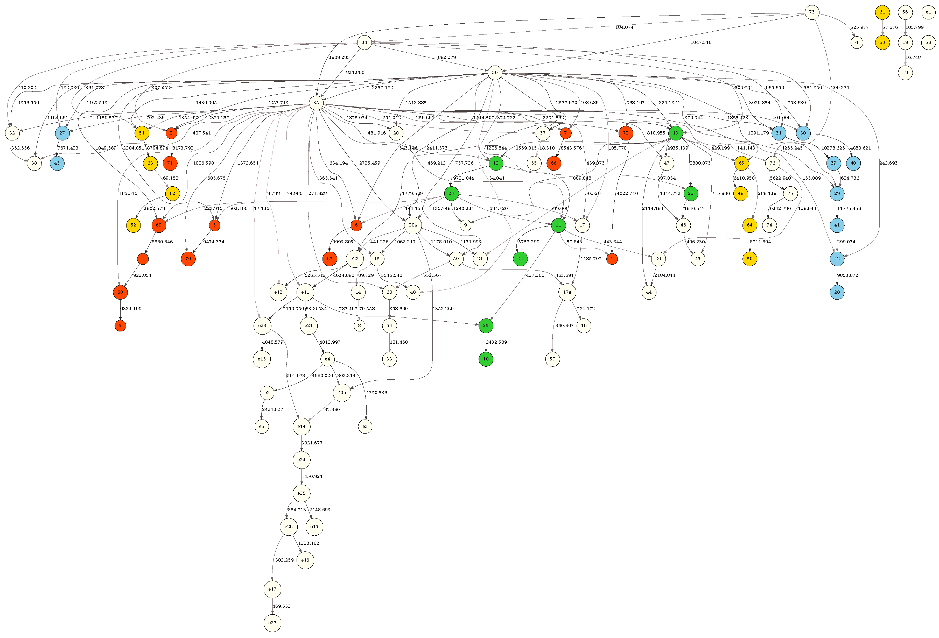
Figure 6.
MDL-based reconstruction of the APOE network. See text for variable descriptions. Shaded nodes and blue edges define the Markov blanket of the target APOE variable. Otherwise, edge color gradient (black to dark to light ochre) corresponds to the edge strength, shown as the number next to the edge. Dotted lines designate the edges missing compared to the full-sample, unstratified network.
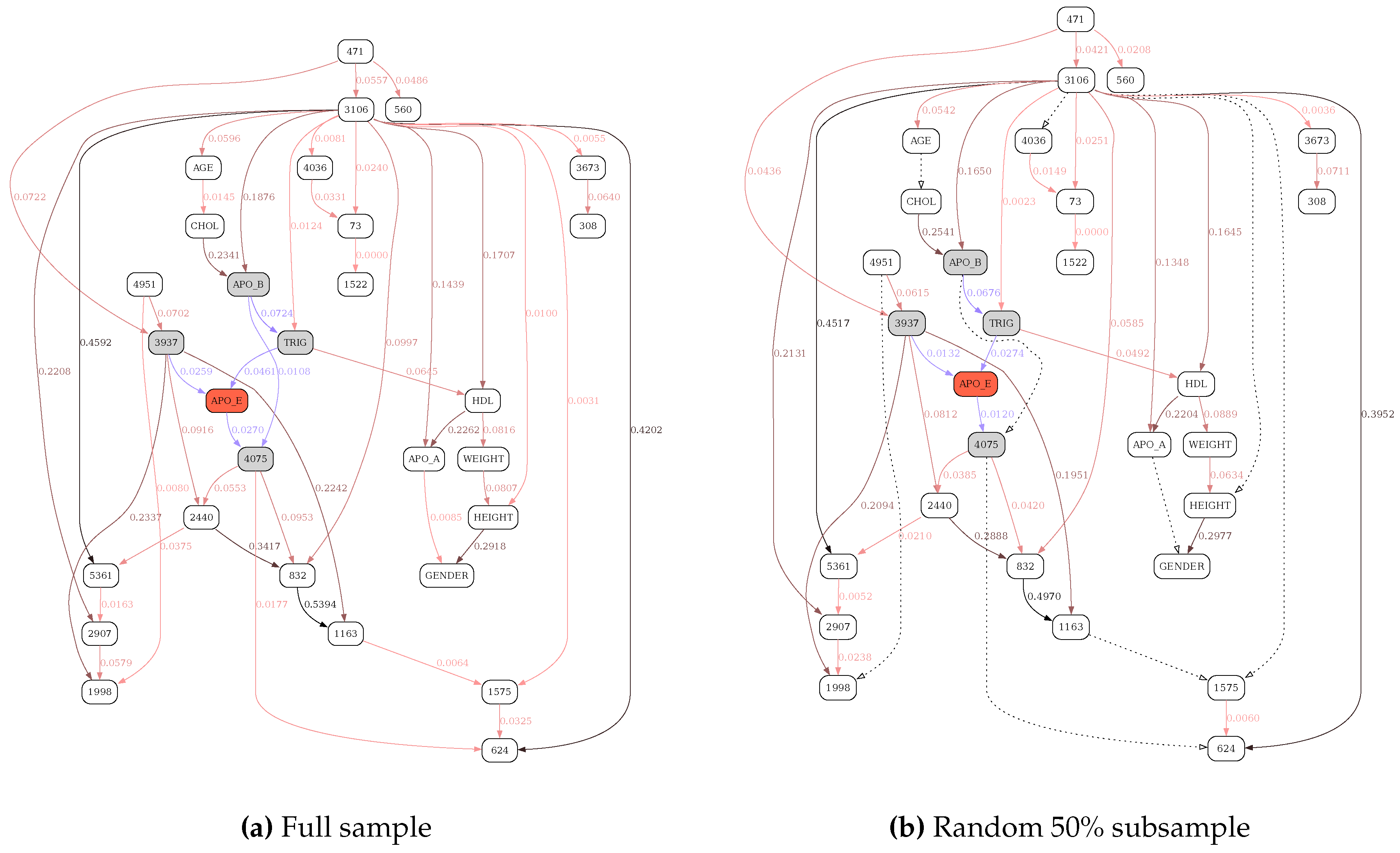
Figure 7.
MDL-based reconstruction of the APOE network, stratified by race. See Figure 6 for further details.
Figure 7.
MDL-based reconstruction of the APOE network, stratified by race. See Figure 6 for further details.
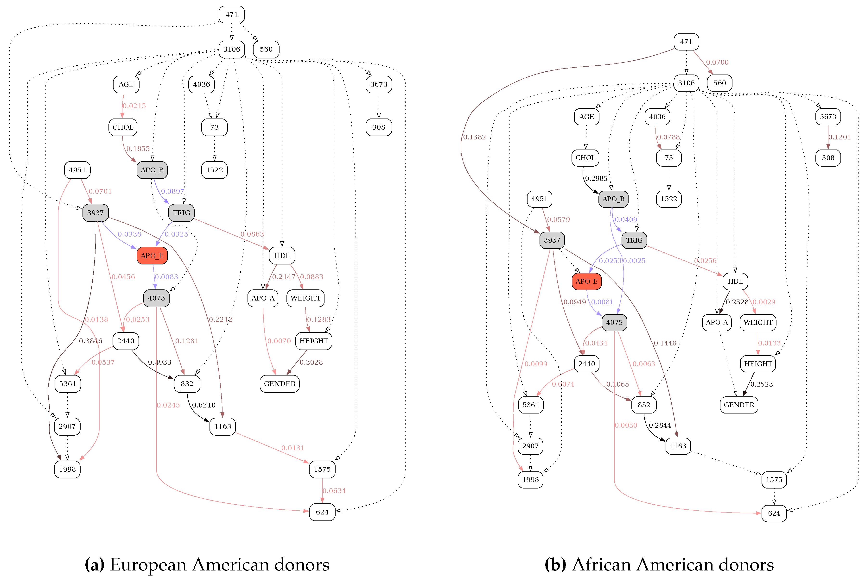
Figure 8.
MU-based reconstruction of the APOE network. See Figure 6 for further details.
Figure 8.
MU-based reconstruction of the APOE network. See Figure 6 for further details.
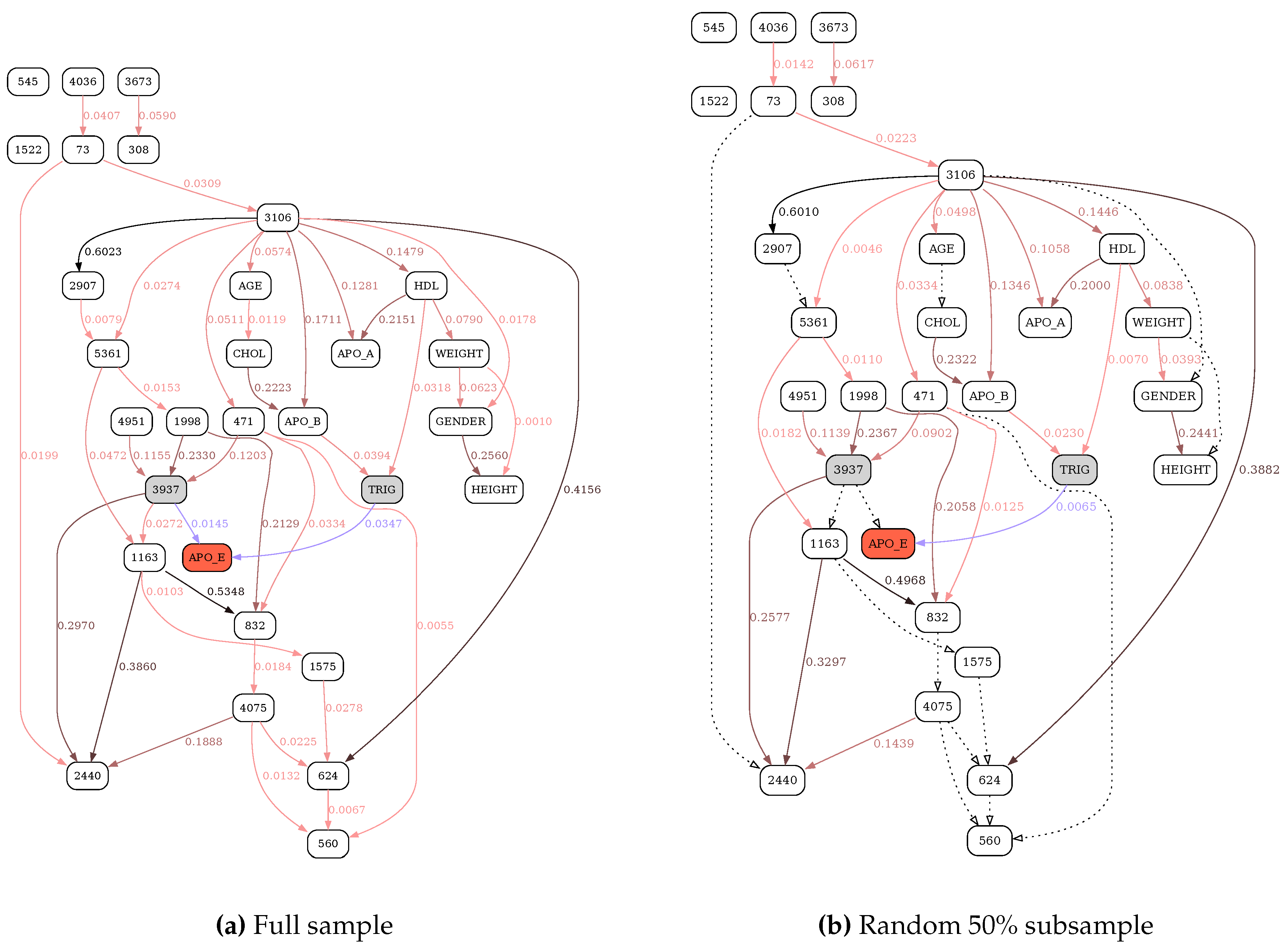
Figure 9.
MU-based reconstruction of the APOE network, stratified by race. See Figure 6 for further details.
Figure 9.
MU-based reconstruction of the APOE network, stratified by race. See Figure 6 for further details.
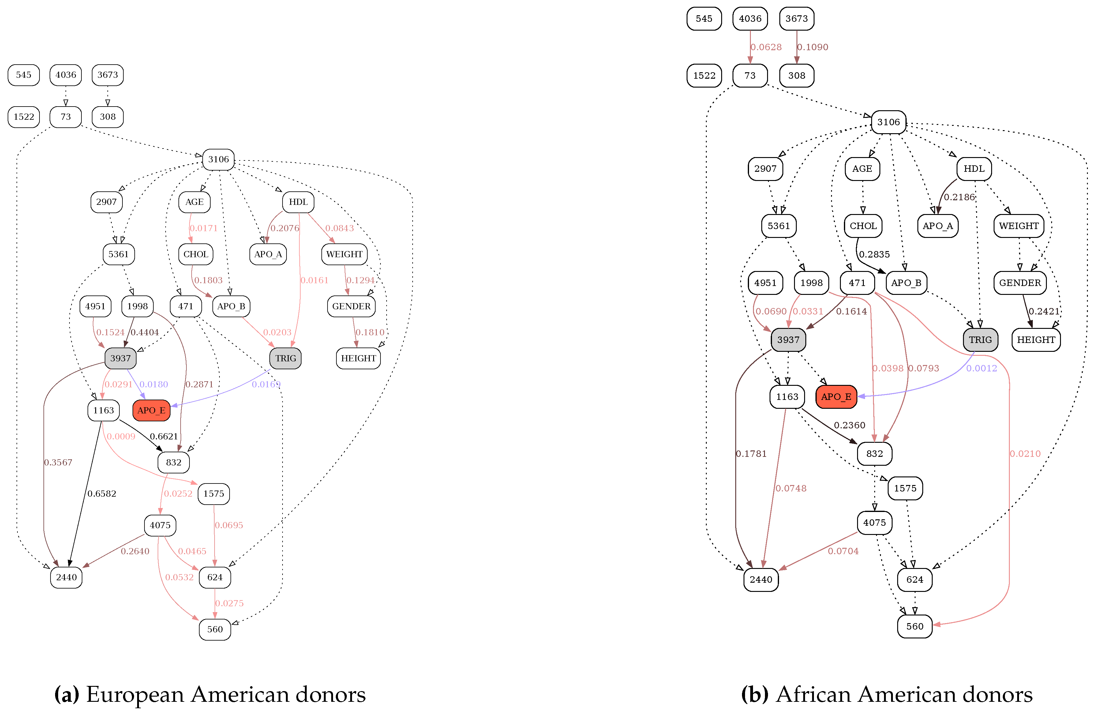
Table 5.
Statistical summary for independent variable pairs with 2 categories and .
| mean | 0.00004980 | 0.00212434 | 0.00046052 | -0.00207455 | -0.00041072 |
| median | 0.00002275 | 0.00215681 | 0.00046052 | -0.00210780 | -0.00043777 |
| 0.00007025 | 0.00008392 | 0.00000000 | 0.00010969 | 0.00007025 | |
| max | 0.00092597 | 0.00218569 | 0.00046052 | -0.00113677 | 0.00046545 |
Table 6.
Statistical summary for independent 4-variate pairs with .
| mean | 0.00045291 | 0.00391531 | 0.00414465 | -0.00346240 | -0.00369174 |
| median | 0.00042035 | 0.00395117 | 0.00414465 | -0.00349716 | -0.00372430 |
| 0.00021309 | 0.00014345 | 0.00000000 | 0.00025671 | 0.00021309 | |
| max | 0.00198022 | 0.00409401 | 0.00414465 | -0.00179072 | -0.00216443 |
Table 7.
Statistical summary for independent 8-variate pairs with .
| mean | 0.00247550 | 0.00722180 | 0.02256533 | -0.00474630 | -0.02008983 |
| median | 0.00244186 | 0.00725890 | 0.02256533 | -0.00478098 | -0.02012347 |
| 0.00049640 | 0.00021950 | 0.00000000 | 0.00054044 | 0.00049640 | |
| max | 0.00532519 | 0.00762947 | 0.02256533 | -0.00136958 | -0.01724014 |
Table 8.
Statistical summary for pairs of 16-variate independent variables with .
| mean | 0.01140676 | 0.01327543 | 0.10361633 | -0.00186866 | -0.09220957 |
| median | 0.01137637 | 0.01331589 | 0.10361633 | -0.00189549 | -0.09223996 |
| 0.00109037 | 0.00032421 | 0.00000000 | 0.00110517 | 0.00109037 | |
| max | 0.01673620 | 0.01408294 | 0.10361633 | 0.00326571 | -0.08688013 |
Table 9.
Statistical summary for pairs of 16-variate independent variables with .
| mean | 0.00112990 | 0.00174350 | 0.01295204 | -0.00061361 | -0.01182214 |
| median | 0.00112681 | 0.00174529 | 0.01295204 | -0.00061679 | -0.01182523 |
| 0.00010648 | 0.00001485 | 0.00000000 | 0.00010760 | 0.00010648 | |
| max | 0.00166940 | 0.00177954 | 0.01295204 | -0.00006718 | -0.01128264 |
Table 10.
Statistical summary of the number of iterations needed by a stochastic hill-climbing search to recover the correct BN structure.
Table 10.
Statistical summary of the number of iterations needed by a stochastic hill-climbing search to recover the correct BN structure.
| Mean | Median | Min | Max | ||
|---|---|---|---|---|---|
| MU iterations | 13.29 | 14.02 | 8 | 2 | 154 |
| MDL iterations | 39.85 | 33.35 | 30 | 2 | 292 |
Disclaimer/Publisher’s Note: The statements, opinions and data contained in all publications are solely those of the individual author(s) and contributor(s) and not of MDPI and/or the editor(s). MDPI and/or the editor(s) disclaim responsibility for any injury to people or property resulting from any ideas, methods, instructions or products referred to in the content. |
© 2024 by the authors. Licensee MDPI, Basel, Switzerland. This article is an open access article distributed under the terms and conditions of the Creative Commons Attribution (CC BY) license (http://creativecommons.org/licenses/by/4.0/).
Copyright: This open access article is published under a Creative Commons CC BY 4.0 license, which permit the free download, distribution, and reuse, provided that the author and preprint are cited in any reuse.


